Embed Size (px)
Citation preview
Carnegie Mellon UniversityResearch Showcase @ CMU
Department of Chemical Engineering Carnegie Institute of Technology
7-2010
Temporal and spatial Lagrangean decompositionsin multi-site, multi-period production planningproblems with sequence-dependent changeoversSebastian Terrazas-MorenoCarnegie Mellon University
Philipp A. TrotterAachen University
Ignacio E. GrossmannCarnegie Mellon University, [email protected]
Follow this and additional works at: http://repository.cmu.edu/cheme
Part of the Chemical Engineering Commons
This Article is brought to you for free and open access by the Carnegie Institute of Technology at Research Showcase @ CMU. It has been accepted forinclusion in Department of Chemical Engineering by an authorized administrator of Research Showcase @ CMU. For more information, pleasecontact [email protected].
Published InComputers and Chemical Engineering, 35, 12, 2913-2928.
* Author to whom correspondence should be addressed. E-mail: [email protected]
Temporal and spatial Lagrangean decompositions in multi-site, multi-period production planning problems with sequence-dependent changeovers Sebastian Terrazas-Morenoa, Philipp Trotterb, Ignacio E. Grossmanna*
aCarnegie Mellon University, 5000 Forbes Ave, Pittsburgh PA 15232, USA, [email protected] bRWTH Aachen University, Templergraben 55, 52056 Aachen, Germany, [email protected] Abstract
We address in this paper the optimization of a multi-site, multi-period, and multi-product
planning problem with sequence-dependent changeovers, which is modeled as a mixed-
integer linear programming (MILP) problem. Industrial instances of this problem require
the planning of a number of production and distribution sites over a time span of several
months. Temporal and spatial Lagrangean decomposition schemes can be useful for
solving these types of large-scale production planning problems. In this paper we present
a theoretical result on the relative size of the duality gap of the two decomposition
alternatives. We also propose a methodology for exploiting the economic interpretation
of the Lagrange multipliers to speed the convergence of numerical algorithms for solving
the temporal and spatial Lagrangean duals. The proposed methods are applied to the
multi-site multi-period planning problem in order to illustrate their computational
effectiveness.
Keywords: Lagrangean decomposition, production planning, temporal decomposition,
spatial decomposition.
1. Introduction
The optimal planning of a network of manufacturing sites and markets is a complex
problem. It involves assigning which products to manufacture in each site, how much to
ship to each market and how much to keep in inventory to satisfy future demand. Each
site has different production capacities and operating costs, while demand for products
varies significantly across markets. Production and distribution planning is concerned
with mid to long-term decisions usually involving several months, adding a temporal
dimension to the spatial distribution given by the multi-site network. The production of
2
each product can involve a setup or cleaning time that in some cases is sequence-
dependent. When setups and sequence-dependent transitions are included, the optimal
planning problem becomes a mixed-integer linear programming (MILP) problem. The
computational expense of solving large-scale MILP problems can be decreased by using
decomposition techniques. This paper presents temporal and spatial Lagrangean
decompositions that allow the independent solution of time periods, production sites, and
markets. The importance of choosing between alternative Lagrangean relaxations of the
same planning model is discussed by Gupta and Maranas (1999). Jackson and Grossmann
(2003) use temporal decomposition for solving a multi-site, multi-period planning
problem. They report that temporal decomposition provides a tighter bound on the full
space solution and has faster dual convergence than spatial decomposition. Wu and
Ierapetritou (2006) also implement Lagrangaen decomposition on a multi-period
scheduling problem. These authors propose to use the Nelder-Mead approach as an
alternative to subgradient method for updating the multipliers. Temporal decomposition
using this approach results in a significant reduction in computational time. Neiro and
Pinto (2006) use temporal Lagrangean decomposition to solve a multi-period MINLP
planning problem under uncertainty concerning a petroleum refinery. They find that this
decomposition scheme helps overcome the exponential increase in solution time that
occurs with the full space model. In a problem similar to the one presented in this paper,
Chen and Pinto (2008) use Lagrangean-based decomposition techniques for solving the
temporal decomposition of a continuous flexible process network. They use subgradient
methods to solve the decomposed problem and find that temporal decomposition
strategies result in a reduction of computational time of several orders of magnitude.
From the papers mentioned above, it is evident that temporal decomposition is an
efficient solution approach for multi-period planning problems. It has been found to
provide a tighter bound on the optimal solution and to have better convergence properties
than Lagrangean spatial decomposition in mulit-site problems. However, there is no
rigorous proof and generalization of the observed result. One objective of this paper is to
compare the bounds obtained through Lagrangean temporal and spatial decompositions
for a class of MILP problems derived from the lot-sizing problem with setup and
sequence-dependent changeover times (Pochet and Wolsey, 2006). The second objective
3
is to use the economic interpretation of the Lagrange multipliers to provide a reduced
dual search space and accelerate the convergence of the optimal multipliers.
This paper is organized as follows. Section 2 presents the details of the MILP
formulation for the production planning problem. Section 3 describes the implementation
of temporal and spatial decomposition of the MILP problem in section 2. In part 4 we
review some important theoretical concepts and in section 5 we introduce a result where
the dual gap of temporal decomposition is found to be at least as small as the dual gap for
spatial decomposition. Sections 6 and 7 contain our novel approach for exploiting the
economic interpretation of the Lagrange multipliers to reduce the search space for the
optimal multipliers. Section 8 presents four numerical examples of increasing size and
complexity for the multi-site multi-period planning problem where the theoretical result
is confirmed, and where the economic interpretation of the multipliers is used to speed
the convergence of numerical algorithms for solving the decomposed problem. Finally,
section 9 presents our conclusions and ideas for future work.
2. Problem Statement
Given is a set of products that are manufactured in several continuous multi-product
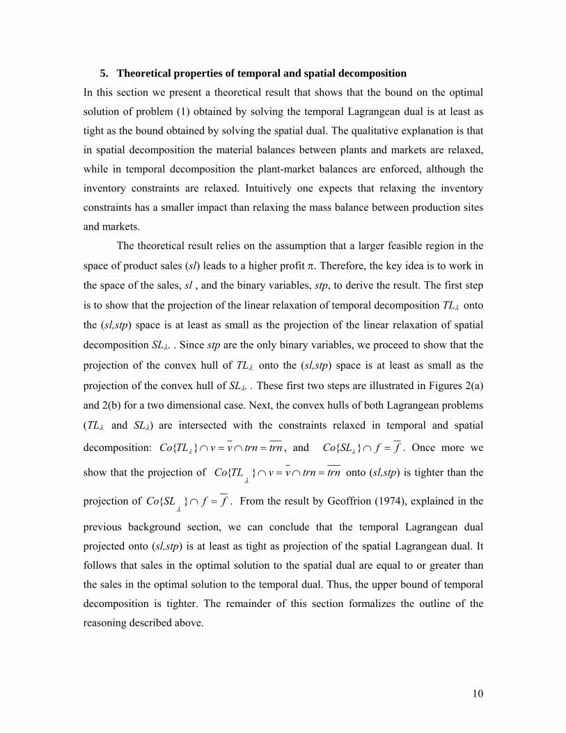
production sites and shipped to a set of markets where they are sold. Let I , S , and M be
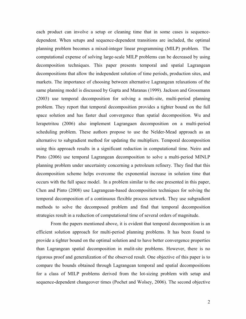
the sets of products, production sites, and markets, respectively. Figure 1 shows the
multi-period, multi-site network structure.
Fig 1. Network of production sites and markets for a multi-period planning problem
Month 1 Month 2 Month n -1 Month n
Multi-site Network
Market 3
Market 2
Market 1
Production Site 1
Production Site 2
Production Site n-1
Production Site n
4
There is a finite time horizon divided into time periods of length tL . The set of
time periods is denoted by T . Given is also a forecast of the demand of each product in
each market at the end of the time periods. The problem is to determine the production in
each site, the inventory levels, and the amounts of products shipped to each market
during each time period in order to maximize the profit. We assume that the size of the
problem may prohibit its direct solution, and we consider that temporal and spatial
Lagrangean decomposition techniques are alternatives to overcome this challenge. One
objective of this work is to rigorously compare the strength of the Lagrangean duals
resulting from each decomposition scheme. Another objective is to illustrate how the
economic interpretation of the Lagrange multipliers of the constraints that are relaxed in
both decompositions can be used to reduce the dual search space.
The following mixed-integer linear programming (MILP) model, which is
formulated in a generic way, corresponds to the profit maximization planning problem
described above.
..
max ,,,
ts
ftrnTCvxslTt Ss
mst
Mm
mst
Tt ss
st
st
st
st
st
st
Tt Ss Mm
mst
mt
(1.1)
SsTt vfxv st
Mm
mst
st
st
,,
1 (1.2)
SsTt stpxx st
UBs
st , (1.3)
SsTt Ltrnbtstpbsxa tst
st
st
st
st
st , (1.4)
SsTt e(trn Ct' )(trn Ct )(stpCs st
s1t
st
st
st
st
st ,) (1.5)
MmSsTt slf ms,t
ms,t ,, (1.6)
MmTt dsl mt
Ss
mst
,, (1.7)
SsTt vv;xx UBs
st
UBs
st , (1.8)
MmSsTt f f UBms,
ms,t ,, (1.9)
SsTt trn,v,x svariable trnI|I|st
|I|st
|I|st
,# (1.10)
MmSsTt sl,f |I|ms,t
|I|ms,t ,, (1.11)
SsTt stp |I|st ,1,0 (1.12)
SsTt 1trnst ,0 (1.13)
5
Equation (1.1) represents the maximization of profit, computed as sales minus
production, inventory, transition, and transportation costs. The coefficients
,,,, st
st
st
mt TC and ms
t, are row vectors of length || I , where I is the set of products
produced and sold in the multi-site network. Equation (1.2) is the production site mass
balance; stx represents production, s
tv inventory levels, and mstf , amount of product
shipped from s to m. Constraint (1.3) enforces the condition that a product can only be
produced if there is a setup assigned to it ( tsstp ). Constraint (1.4) limits the time balance
at each production site involving the transition variables tstrn . The row vector s
ta
contains the inverse of the production rates of all products, while stbs and s
tbt are vectors
with set up and transition times. tL is the duration of time period t. Constraint (1.5) is a
compact representation of a set of general sequencing constraints. In general, assume
there are Kk ,...,1 constraints in this set. Then stCs is a matrix with K rows and I
columns, and stCt and s
tCt' are matrices with the same number of rows and II (#
trn variables) columns. The expression # trn variables represents the different types of
transition variables used in the model, for instance, transition within time periods,
transitions across time periods, etc. The vector of right hand side coefficients ste has
dimension K . Equation (1.6) expresses the condition that all products that arrive to a
market are sold. The vector mtd contains the market demands for all the products at each
time period. The rest of the constraints involve the upper bounds, ranges, and integrality
conditions of the decision variables. It is important to note that the transition variables
tstrn are continuous and bounded between zero and one. We assume that constraint (1.5)
contains sequencing constraints of the type shown in Appendix A and proposed by
Erdirik-Dogan and Grossmann (2008), where transition variables always take values of 0
or 1, even if they are declared as continuous.
The explicit model used for the examples included in this paper is shown in Appendix A.
6
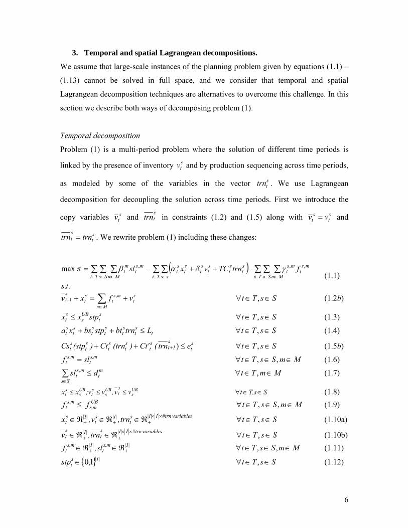
3. Temporal and spatial Lagrangean decompositions.
We assume that large-scale instances of the planning problem given by equations (1.1) –
(1.13) cannot be solved in full space, and we consider that temporal and spatial
Lagrangean decomposition techniques are alternatives to overcome this challenge. In this
section we describe both ways of decomposing problem (1).
Temporal decomposition
Problem (1) is a multi-period problem where the solution of different time periods is
linked by the presence of inventory stv and by production sequencing across time periods,
as modeled by some of the variables in the vector sttrn . We use Lagrangean
decomposition for decoupling the solution across time periods. First we introduce the
copy variables stv and
sttrn in constraints (1.2) and (1.5) along with s
ts
t vv and
st
st trntrn . We rewrite problem (1) including these changes:
..
max ,,,
ts
ftrnTCvxsl Tt Ss
mst
Mm
mst
Tt ss
st
st
st
st
st
st
Tt Ss Mm
mst
mt
(1.1)
SsTtvfxv st
Mm
mst
st
st
, ,1 (1.2b)
SsTt stpxx st
UBs
st , (1.3)
SsTt Ltrnbtstpbsxa tst
st
st
st
st
st , (1.4)
SsTt etrn( Ct' )(trn Ct )(stpCs st
s1t
st
st
st
st
st ,) (1.5b)
MmSsTt slf ms,t
ms,t ,, (1.6)
MmTt dsl mt
Ss
mst
,, (1.7)
ST,st vv,v;vxx UBs
st
UBs
st
UBs
st (1.8)
MmSsTt f f UBms,
ms,t ,, (1.9)
SsTt trn,v,x svariable trnI|I|st
|I|st
|I|st
,# (1.10a)
SsTt trn,v svariable trnI|I|st
|I|st
,# (1.10b)
MmSsTt sl,f |I|ms,t
|I|ms,t ,, (1.11)
SsTt stp |I|st ,1,0 (1.12)
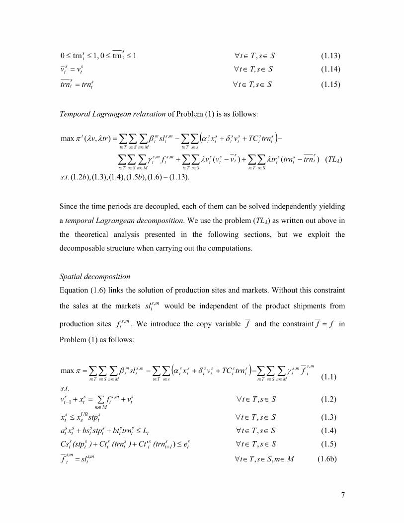
7
SsTt , 1trn0 1,trn0st
st (1.13)
SsT,t vv st
st (1.14)
SsT,t trntrn st
st (1.15)
Temporal Lagrangean relaxation of Problem (1) is as follows:
).13.1()6.1(),5.1(),4.1(),3.1(),2.1( ..
)()(
),( max
,,
,
bbts
trntrntrvvvf
trnTCvxsltrv
st
st
Tt Ss
st
st
st
Tt Ss
st
Tt Ss
mst
Mm
mst
Tt ss
st
st
st
st
st
st
Tt Ss Mm
mst
mt
t
(TL)
Since the time periods are decoupled, each of them can be solved independently yielding
a temporal Lagrangean decomposition. We use the problem (TL) as written out above in
the theoretical analysis presented in the following sections, but we exploit the
decomposable structure when carrying out the computations.
Spatial decomposition
Equation (1.6) links the solution of production sites and markets. Without this constraint
the sales at the markets mstsl , would be independent of the product shipments from
production sites mstf
, . We introduce the copy variable f and the constraint ff in
Problem (1) as follows:
..
max,,,
ts
ftrnTCvxslTt Ss
ms
tMm
mst
Tt ss
st
st
st
st
st
st
Tt Ss Mm
mst
mt
(1.1)
SsTt vfxv st
Mm
mst
st
st
,,
1 (1.2)
SsTt stpxx st
UBs
st , (1.3)
SsTt Ltrnbtstpbsxa tst
st
st
st
st
st , (1.4)
SsTt e(trn Ct' )(trn Ct )(stpCs st
s1t
st
st
st
st
st ,) (1.5)
MmSsTt slf ms,t
ms,
t ,, (1.6b)
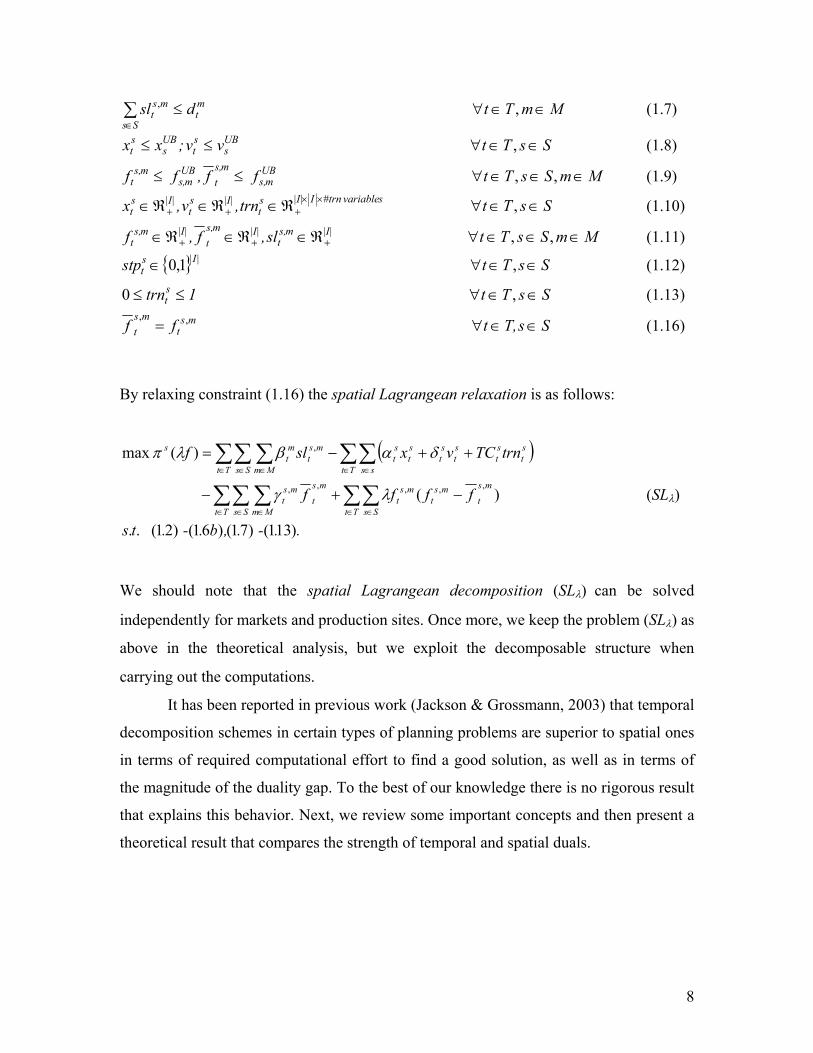
8
MmTt dsl mt
Ss
mst
,, (1.7)
SsTt vv;xx UBs
st
UBs
st , (1.8)
MmSsTt f f,f f UBms,
ms,
tUBms,
ms,t ,, (1.9)
SsTt trn,v,x svariable trnI|I|st
|I|st
|I|st
,# (1.10)
MmSsTt sl,f,f |I|ms,t
|I|ms,
t|I|ms,
t ,, (1.11)
SsTt stp |I|st ,1,0 (1.12)
SsTt 1trnst ,0 (1.13)
SsT,t ff mst
ms
t ,, (1.16)
By relaxing constraint (1.16) the spatial Lagrangean relaxation is as follows:
.. -.,b. -. ts
ffff
trnTCvxslf
Tt Ss
ms
tms
tms
tTt Ss
ms
tMm
mst
Tt ss
st
st
st
st
st
st
Tt Ss Mm
mst
mt
s
)131()71()61()21( ..
)(
)( max
,,,,,
,
(SL)
We should note that the spatial Lagrangean decomposition (SLcan be solved
independently for markets and production sites. Once more, we keep the problem (SL) as
above in the theoretical analysis, but we exploit the decomposable structure when
carrying out the computations.
It has been reported in previous work (Jackson & Grossmann, 2003) that temporal
decomposition schemes in certain types of planning problems are superior to spatial ones
in terms of required computational effort to find a good solution, as well as in terms of
the magnitude of the duality gap. To the best of our knowledge there is no rigorous result
that explains this behavior. Next, we review some important concepts and then present a
theoretical result that compares the strength of temporal and spatial duals.
9
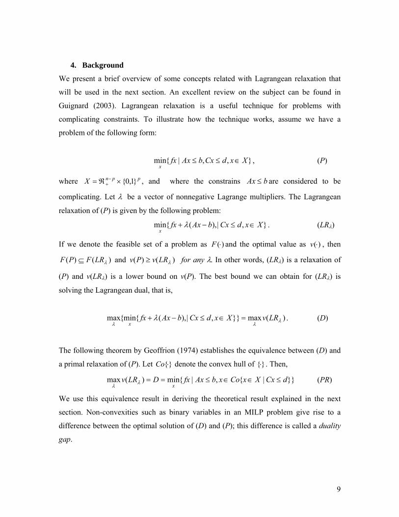
4. Background
We present a brief overview of some concepts related with Lagrangean relaxation that
will be used in the next section. An excellent review on the subject can be found in
Guignard (2003). Lagrangean relaxation is a useful technique for problems with
complicating constraints. To illustrate how the technique works, assume we have a
problem of the following form:
},,|{min XxdCxbAxfxx
, (P)
where ppnX }1,0{ , and where the constrains bAx are considered to be
complicating. Let be a vector of nonnegative Lagrange multipliers. The Lagrangean
relaxation of (P) is given by the following problem:
},|),({min XxdCxbAxfxx
. (LR)
If we denote the feasible set of a problem as )(F and the optimal value as )(v , then
)()( LRFPF and )()( LRvPv for any In other words, (LR) is a relaxation of
(P) and v(LR) is a lower bound on v(P). The best bound we can obtain for (LR) is
solving the Lagrangean dual, that is,
)(max}},|),({min{max
LRvXxdCxbAxfxx
. (D)
The following theorem by Geoffrion (1974) establishes the equivalence between (D) and
a primal relaxation of (P). Let }{Co denote the convex hull of }{ . Then,
}}|{,|{min)(max dCxXxCoxbAxfxDLRvx
(PR)
We use this equivalence result in deriving the theoretical result explained in the next
section. Non-convexities such as binary variables in an MILP problem give rise to a
difference between the optimal solution of (D) and (P); this difference is called a duality
gap.
10
5. Theoretical properties of temporal and spatial decomposition
In this section we present a theoretical result that shows that the bound on the optimal
solution of problem (1) obtained by solving the temporal Lagrangean dual is at least as
tight as the bound obtained by solving the spatial dual. The qualitative explanation is that
in spatial decomposition the material balances between plants and markets are relaxed,
while in temporal decomposition the plant-market balances are enforced, although the
inventory constraints are relaxed. Intuitively one expects that relaxing the inventory
constraints has a smaller impact than relaxing the mass balance between production sites
and markets.
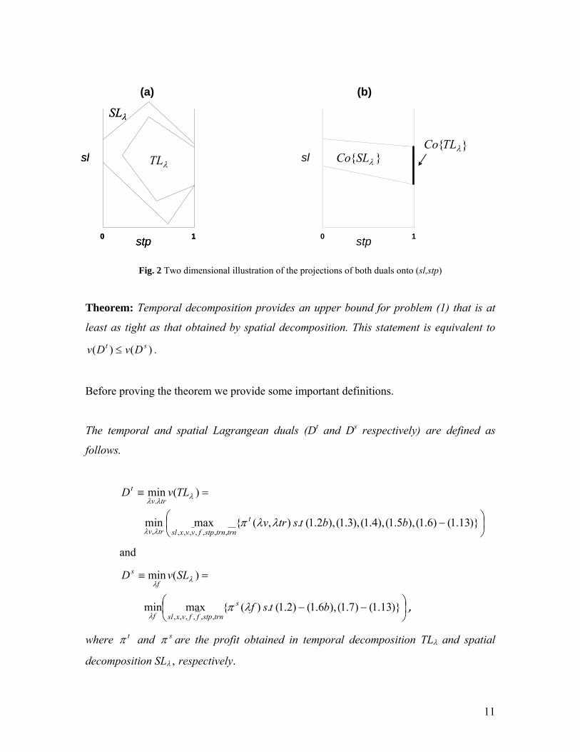
The theoretical result relies on the assumption that a larger feasible region in the
space of product sales (sl) leads to a higher profit . Therefore, the key idea is to work in
the space of the sales, sl , and the binary variables, stp, to derive the result. The first step
is to show that the projection of the linear relaxation of temporal decomposition TL onto
the (sl,stp) space is at least as small as the projection of the linear relaxation of spatial
decomposition SL. . Since stp are the only binary variables, we proceed to show that the
projection of the convex hull of TL onto the (sl,stp) space is at least as small as the
projection of the convex hull of SL These first two steps are illustrated in Figures 2(a)
and 2(b) for a two dimensional case. Next, the convex hulls of both Lagrangean problems
(TL and SLare intersected with the constraints relaxed in temporal and spatial
decomposition: trntrnvvTLCo }{ , and ffSLCo }{ . Once more we
show that the projection of trntrnvvTLCo }{
onto (sl,stp) is tighter than the
projection of ffSLCo }{
. From the result by Geoffrion (1974), explained in the
previous background section, we can conclude that the temporal Lagrangean dual
projected onto (sl,stp) is at least as tight as projection of the spatial Lagrangean dual. It
follows that sales in the optimal solution to the spatial dual are equal to or greater than
the sales in the optimal solution to the temporal dual. Thus, the upper bound of temporal
decomposition is tighter. The remainder of this section formalizes the outline of the
reasoning described above.
11
Fig. 2 Two dimensional illustration of the projections of both duals onto (sl,stp)
Theorem: Temporal decomposition provides an upper bound for problem (1) that is at
least as tight as that obtained by spatial decomposition. This statement is equivalent to
)()( st DvDv .
Before proving the theorem we provide some important definitions.
The temporal and spatial Lagrangean duals (Dt and Ds respectively) are defined as
follows.
)}13.1()6.1(),5.1(),4.1(),3.1(),2.1(.),({maxmin
)(min
,,,,,,,,
.
bbtstrv
TLvD
t
trntrnstpfvvxsltrv
trv
t
and
,
)}13.1()7.1(),6.1()2.1(.)({maxmin
)(min
,,,,,,btsf
SLvD
s
trnstpffvxslf
f
s
where t and s are the profit obtained in temporal decomposition TLand spatial
decomposition SLrespectively.
sl
stp 0 1
SL
TL sl
stp 0 1
SL
sl
stp0 1
}{ SLCo
}{ TLCo
(a) (b)
12
FLP is the linear programming relaxation of F.
FtrnstpfvxslstpslFprojpF stpsl ),,,,,(:),(, , is the projection of F onto
the space of product sales and binary variables (set-ups).
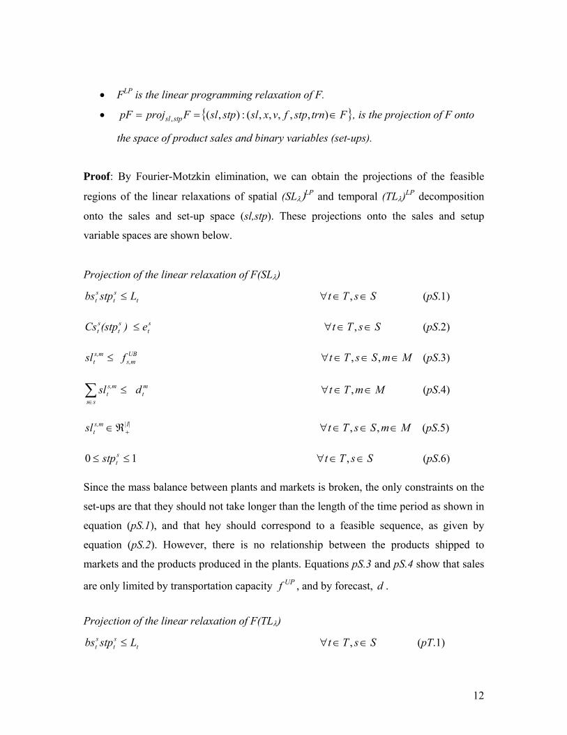
Proof: By Fourier-Motzkin elimination, we can obtain the projections of the feasible
regions of the linear relaxations of spatial (SLLP and temporal (TL)LP decomposition
onto the sales and set-up space (sl,stp). These projections onto the sales and setup
variable spaces are shown below.
Projection of the linear relaxation of F(SL)
SsTt Lstpbs tst
st , (pS.1)
SsTte) (stpCs s
tst
st , (pS.2)
MmSsTt fsl UB
s,ms,mt ,, (pS.3)
MmTt dsl m
tss
s,mt
, (pS.4)
MmSsTtsl |I|s,m
t ,, (pS.5)
SsTt stps
t , 10 (pS.6)
Since the mass balance between plants and markets is broken, the only constraints on the
set-ups are that they should not take longer than the length of the time period as shown in
equation (pS.1), and that hey should correspond to a feasible sequence, as given by
equation (pS.2). However, there is no relationship between the products shipped to
markets and the products produced in the plants. Equations pS.3 and pS.4 show that sales
are only limited by transportation capacity UPf , and by forecast, d .
Projection of the linear relaxation of F(TL)
SsTt Lstpbs tst
st , (pT.1)
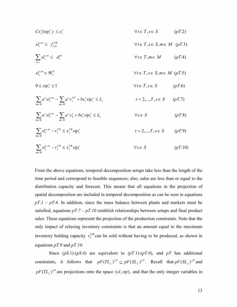
13
SsTte) (stpCs st
st
st , (pT.2)
MmSsTt fsl UB
s,ms,mt ,, (pT.3)
MmTt dsl m
tss
s,mt
, (pT.4)
MmSsTt sl |I|s,m
t ,, (pT.5)
SsTt stps
t , 10 (pT.6)
SsTt Lstpbsvasla t
st
st
Mm
UPs
s
Mm
s,mt
s
,,...,2 (pT.7)
Ss Lstpbsvasla ss
Mm
ss
Mm
s,ms
11101 (pT.8)
SsTtstpxvsl s
tUBs
UBs
Mm
mst
,,...,2 , (pT.9)
Ssstpxvsl sUB
sUBs
Mm
ms
1,
1 (pT.10)
From the above equations, temporal decomposition setups take less than the length of the
time period and correspond to feasible sequences; also, sales are less than or equal to the
distribution capacity and forecast. This means that all equations in the projection of
spatial decomposition are included in temporal decomposition as can be seen in equations
pT.1 – pT.6. In addition, since the mass balance between plants and markets must be
satisfied, equations pT.7 – pT.10 establish relationships between setups and final product
sales. These equations represent the projection of the production constraints. Note that the
only impact of relaxing inventory constraints is that an amount equal to the maximum
inventory holding capacity UBsv can be sold without having to be produced, as shown in
equations pT.9 and pT.10.
Since (pS.1)-(pS.6) are equivalent to (pT.1)-(pT.6), and pT has additional
constraints, it follows that LPLP SLpFTLpF )()( . Recall that LPSLpF )( and
LPTLpF )( are projections onto the space ),( stpsl , and that the only integer variables in
14
the MILP problem are the setup variables stp . Therefore, we can establish the following
implication:
}{}{)()( SLpCoTLpCoSLpFTLpF LPLP . (4)
Now, constraint (1.6) in the temporal Lagrangean relaxation, TL , allows us to make the
following statement: }:),{(),()(),( fslfslfslTLFfsl ,
or equivalently, },:),,{(),,()(),( fffslffslffslTLFfsl .
This statement together with (4) gives:
)}]:),{(}{[}{ ffffSLCopTLpCo . (5)
If the right-hand-side of expression (5) remains unchanged, any set obtained by
restricting the left-hand-side is still a subset of the right-hand side. Thus, we can state
that:
}]:),{(}{[}],:),,,{(}{[ ffffSLCopvvtrntrnvvtrntrnTLCop .
(6)
According to the equivalence result of Geoffrion (1974),
)(},:),,,{(}{ tDFvvtrntrnvvtrntrnTLCo (7)
and
)(}:),{(}{ sDFffffSLCo (8)
From (7) and (8), we can restate (6) as follows,
)]([)]([ st DFpDFp . (9)
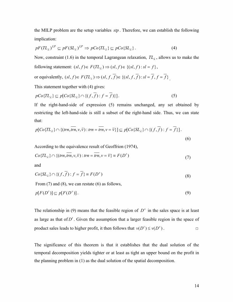
The relationship in (9) means that the feasible region of sD in the sales space is at least
as large as that of tD . Given the assumption that a larger feasible region in the space of
product sales leads to higher profit, it then follows that )()( st DvDv . □
The significance of this theorem is that it establishes that the dual solution of the
temporal decomposition yields tighter or at least as tight an upper bound on the profit in
the planning problem in (1) as the dual solution of the spatial decomposition.
15
6. An accelerating technique for the solution of (TL) and (SL)
While the theoretical results in the first part of this paper support the use of temporal
decomposition, we focus in this part in ways of selecting the Lagrange multipliers in
order to accelerate the convergence in both temporal and spatial decompositions. The
general idea is to use the economic interpretation of the Lagrange multipliers to limit
their search space by setting upper and lower bounds on their possible values. The
economic interpretation of the Lagrange multipliers, or dual variables, in linear
programming (LP) is well understood (Dorfman et al., 1958; Chvátal, 1983). Williams
(1996) expanded these ideas to mixed integer programming. In this work, we exploit the
economic interpretation of Lagrange multipliers given in LP duality theory. We use this
interpretation to set bounds on the possible values of the Lagrange multipliers of some of
the constraints relaxed in temporal decomposition (TL) and spatial decomposition (SL).
Since the constraints that we consider here are written only in terms of continuous
variables, we propose to use these bounds even if (TL) and (SL) are MILP problems.
This idea is developed and discussed in great detail in Trotter (2009. First, we review the
interpretation of the Lagrange multipliers as dual variables in a linear programming
problem. Then, we explain how to exploit the economic interpretation of the dual
variables of the relaxed constraints to set valid bounds for the magnitude of the Lagrange
multipliers. The role of the set of active constraints is explored by analyzing two limiting
scenarios: sales are limited by production capacity, and sales are limited by market
demand. In each scenario the set of active constraints in planning problem (1) is different,
and thus, the values of the optimal Lagrange multipliers are also different.
Lagrange multipliers as dual variables
Consider the optimization problem (P):
},,|{min XxdCxbAxxx
. (P)
The Lagrangean relaxation of (P) is:
},|),({min XxdCxbAxxx
. (LR)
Let x be the production of a certain good and φ its cost. The Lagrange multiplier λ in
(LRλ) imposes a penalty for violating constraint bAx in (P). In duality theory, λ is the
16
dual variable associated with constraint bAx ; the optimal value of the dual variable,
represents the added value if constraint bAx is violated by one unit, and if the optimal
active set remains the same. If (LRλ) is linear and continuous, and λ is set to the optimal
value of the dual variable associated with bAx , then the optimal value of (P) and (LRλ)
are the same. This last result does not hold, in general, for mixed-integer linear
programming (MILP) problems. In this case the optimal value of (LR) is generally larger
than the optimal value of (P). Since the Lagrange multiplier is still a penalty for the
violation of constraint bAx . Given the structure of problem (1), we propose to use the
economic interpretation of the dual variables of its linear relaxation , as a basis for setting
bounds on the optimal penalty λ in (LRλ), even if our problem is an MILP.
Economic interpretation of the Lagrange multipliers
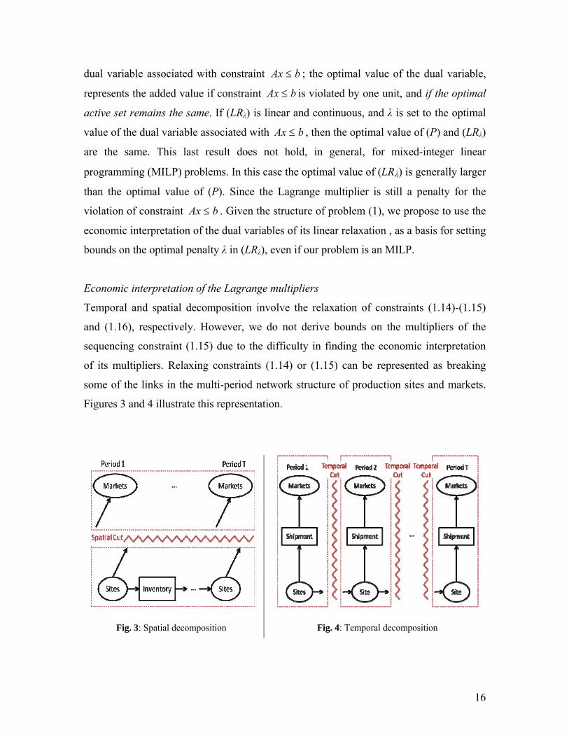
Temporal and spatial decomposition involve the relaxation of constraints (1.14)-(1.15)
and (1.16), respectively. However, we do not derive bounds on the multipliers of the
sequencing constraint (1.15) due to the difficulty in finding the economic interpretation
of its multipliers. Relaxing constraints (1.14) or (1.15) can be represented as breaking
some of the links in the multi-period network structure of production sites and markets.
Figures 3 and 4 illustrate this representation.
Fig. 3: Spatial decomposition
Fig. 4: Temporal decomposition
17
When temporal decomposition is considered, in order to penalize the violation of
constraint (1.14), the term )( st
st
Tt Ss
st vvv
is added to the objective function of TLλ.
The multipliers stv act as a selling price for s
tv or a buying price for stv in a hypothetical
external market. Our main idea in this section of the paper is that there is a market price
stv that makes the profit in the decomposed system in Figure 4 very similar to the profit
in the original, full space, planning problem (1). For instance, if integer variables are
relaxed or eliminated from (1), a market value stv equal to the optimal dual variable of
(1.14) would result in the same profit for temporal decomposition TLλ and for problem
(1). Similarly, in the objective function of spatial decomposition SLλ, ms
tf , represents the
selling price of mstf , and the buying price of
ms
tf,
in a hypothetical external market.
Our objective is to find the market values for stv , s
tv , ms
tf,
, and mstf , that make
the optimal value of (TLλ) and (SLλ) as close as possible to the optimal value of problem
(1). Notice that, since (1) is an MILP problem, there is a duality gap that prevents the
optimal values of TLλ and SLλ to be identical to the solution of problem (1).
The set of active constraints in the optimal solution to Problem (1) results in
different market prices stv and ms
tf , in the decomposed problems. Since, in general, it
is impossible to know the optimal active set a priori, we analyze two extreme scenarios
that correspond to completely different active sets, and determine the corresponding
market prices stv and ms
tf , . The two scenarios that we propose for problem (1) are the
following: (a) the market demand exceeds the production capacity of the manufacturing
sites for all time periods, and (b) the production capacity exceeds the market demand for
every time period. The market values for these two extreme cases are used to set
rigorous bounds on the multipliers as described below.
To find the upper bounds on the multipliers we use a value chain representation of
the multi-site, multi-period network. For instance, assume that products in the network
flow from stage 0 to stage i, and then from node i to node n. The flow through each of
these stages, or nodes, adds value to the products; the collection of value-adding stages in
18
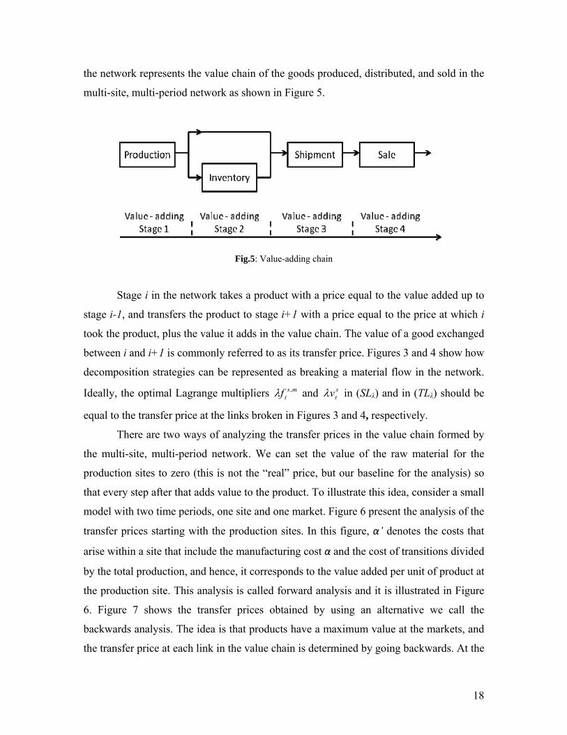
the network represents the value chain of the goods produced, distributed, and sold in the
multi-site, multi-period network as shown in Figure 5.
Fig.5: Value-adding chain
Stage i in the network takes a product with a price equal to the value added up to
stage i-1, and transfers the product to stage i+1 with a price equal to the price at which i
took the product, plus the value it adds in the value chain. The value of a good exchanged
between i and i+1 is commonly referred to as its transfer price. Figures 3 and 4 show how
decomposition strategies can be represented as breaking a material flow in the network.
Ideally, the optimal Lagrange multipliers mstf , and s
tv in (SLλ) and in (TLλ) should be
equal to the transfer price at the links broken in Figures 3 and 4, respectively.
There are two ways of analyzing the transfer prices in the value chain formed by
the multi-site, multi-period network. We can set the value of the raw material for the
production sites to zero (this is not the “real” price, but our baseline for the analysis) so
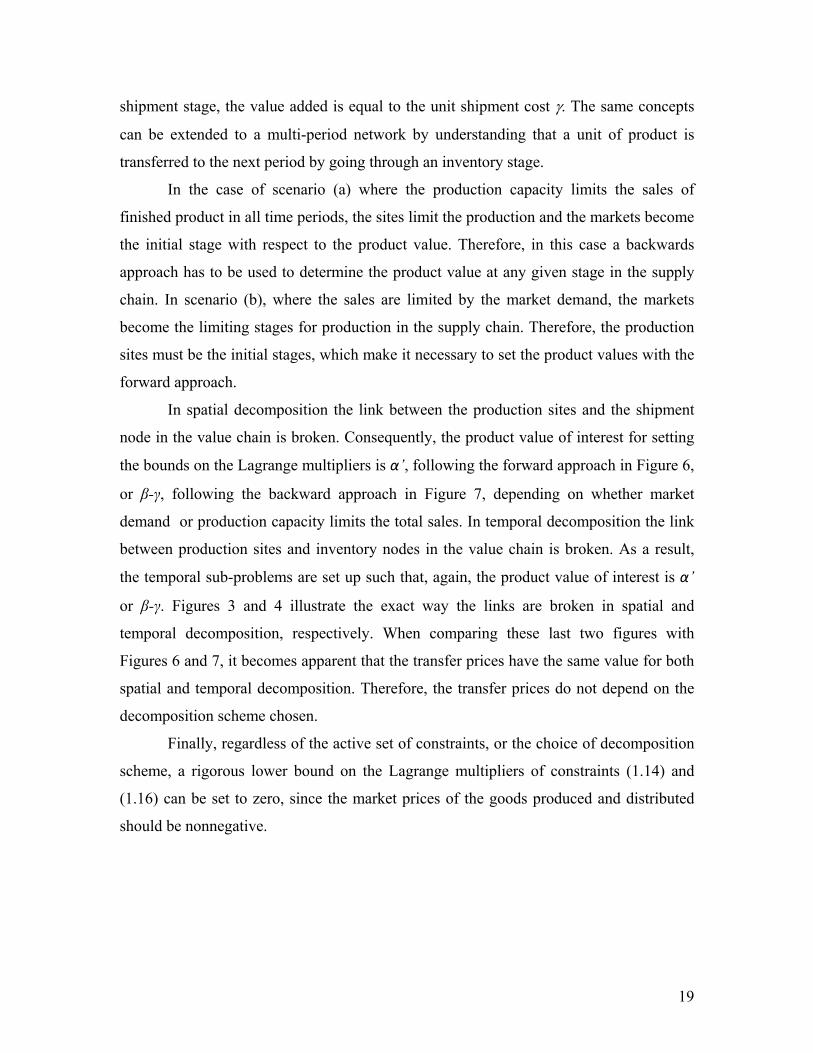
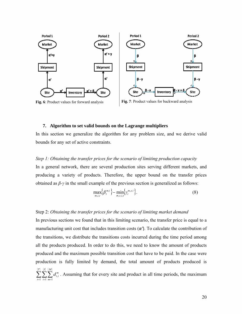
that every step after that adds value to the product. To illustrate this idea, consider a small
model with two time periods, one site and one market. Figure 6 present the analysis of the
transfer prices starting with the production sites. In this figure, α’ denotes the costs that
arise within a site that include the manufacturing cost α and the cost of transitions divided
by the total production, and hence, it corresponds to the value added per unit of product at
the production site. This analysis is called forward analysis and it is illustrated in Figure
6. Figure 7 shows the transfer prices obtained by using an alternative we call the
backwards analysis. The idea is that products have a maximum value at the markets, and
the transfer price at each link in the value chain is determined by going backwards. At the
19
shipment stage, the value added is equal to the unit shipment cost . The same concepts
can be extended to a multi-period network by understanding that a unit of product is
transferred to the next period by going through an inventory stage.
In the case of scenario (a) where the production capacity limits the sales of
finished product in all time periods, the sites limit the production and the markets become
the initial stage with respect to the product value. Therefore, in this case a backwards
approach has to be used to determine the product value at any given stage in the supply
chain. In scenario (b), where the sales are limited by the market demand, the markets
become the limiting stages for production in the supply chain. Therefore, the production
sites must be the initial stages, which make it necessary to set the product values with the
forward approach.
In spatial decomposition the link between the production sites and the shipment
node in the value chain is broken. Consequently, the product value of interest for setting
the bounds on the Lagrange multipliers is α’, following the forward approach in Figure 6,
or β-γ, following the backward approach in Figure 7, depending on whether market
demand or production capacity limits the total sales. In temporal decomposition the link
between production sites and inventory nodes in the value chain is broken. As a result,
the temporal sub-problems are set up such that, again, the product value of interest is α’
or β-γ. Figures 3 and 4 illustrate the exact way the links are broken in spatial and
temporal decomposition, respectively. When comparing these last two figures with
Figures 6 and 7, it becomes apparent that the transfer prices have the same value for both
spatial and temporal decomposition. Therefore, the transfer prices do not depend on the
decomposition scheme chosen.
Finally, regardless of the active set of constraints, or the choice of decomposition
scheme, a rigorous lower bound on the Lagrange multipliers of constraints (1.14) and
(1.16) can be set to zero, since the market prices of the goods produced and distributed
should be nonnegative.
20
7. Algorithm to set valid bounds on the Lagrange multipliers
In this section we generalize the algorithm for any problem size, and we derive valid
bounds for any set of active constraints.
Step 1: Obtaining the transfer prices for the scenario of limiting production capacity
In a general network, there are several production sites serving different markets, and
producing a variety of products. Therefore, the upper bound on the transfer prices
obtained as β-γ in the small example of the previous section is generalized as follows:
s,imt
tism
m,it
timγβ ,
,,,,,minmax . (8)
Step 2: Obtaining the transfer prices for the scenario of limiting market demand
In previous sections we found that in this limiting scenario, the transfer price is equal to a
manufacturing unit cost that includes transition costs (α’). To calculate the contribution of
the transitions, we distribute the transitions costs incurred during the time period among
all the products produced. In order to do this, we need to know the amount of products
produced and the maximum possible transition cost that have to be paid. In the case were
production is fully limited by demand, the total amount of products produced is
T
t
I
i
M
m
mitd
1 1 1, . Assuming that for every site and product in all time periods, the maximum
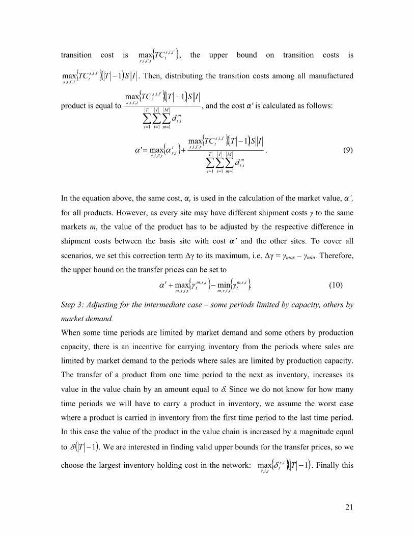
Fig. 6: Product values for forward analysis
Fig. 7: Product values for backward analysis
21
transition cost is ',,
,',,max iis
ttiis
TC , the upper bound on transition costs is
ISTTC iist
tiis1max ',,
,',, . Then, distributing the transition costs among all manufactured
product is equal to
T
t
I
i
M
m
mit
iist
tiis
d
ISTTC
1 1 1,
',,
,',,1max
, and the cost α’ is calculated as follows:
T
t
I
i
M
m
mit
iist
tiistis
tiis
d
ISTTC
1 1 1,
',,
,',,,
,',,
1maxmax' . (9)
In the equation above, the same cost, α, is used in the calculation of the market value, α’,
for all products. However, as every site may have different shipment costs γ to the same
markets m, the value of the product has to be adjusted by the respective difference in
shipment costs between the basis site with cost α’ and the other sites. To cover all
scenarios, we set this correction term Δγ to its maximum, i.e. Δγ = γmax – γmin. Therefore,
the upper bound on the transfer prices can be set to
.minmax ,
,,,
,,
,,,
im,st
tism
ismt
tismγ (10)
Step 3: Adjusting for the intermediate case – some periods limited by capacity, others by
market demand.
When some time periods are limited by market demand and some others by production
capacity, there is an incentive for carrying inventory from the periods where sales are
limited by market demand to the periods where sales are limited by production capacity.
The transfer of a product from one time period to the next as inventory, increases its
value in the value chain by an amount equal to Since we do not know for how many
time periods we will have to carry a product in inventory, we assume the worst case
where a product is carried in inventory from the first time period to the last time period.
In this case the value of the product in the value chain is increased by a magnitude equal
to 1T . We are interested in finding valid upper bounds for the transfer prices, so we
choose the largest inventory holding cost in the network: 1max ,
,,Tis
ttis . Finally this

22
term is added to the formula for obtaining an upper bound on the transfer price in (a) the
limiting production capacity case, and (b) the limiting market demand case.
(a)
1maxminmax ,
,,
,
,,,,,
lim TγβUP ist
tis
im,st
tism
m,it
timcapacity (11)
(b)
1maxminmax
1maxmax
,,,,,,,,
1 1 1,
',,
,',,
,,
lim
Tδγγ
d
ISTTCαUP
s,it
tis
m,s,it
tism
m,s,it
tism
T
t
I
i
M
m
mit
iist
tiists,i
tisdemand
(12)
Step 4: Solving the linear relaxation of Problem (1)
It is impossible to know the complete active set of planning problem (1) before solving it.
However, it is possible to infer from the linear relaxation some useful information. The
change from fractional to integral variables in (1.4) either reduces or does not change the
amount of products that can be produced. Therefore, if the production time constraint
(1.4) is active for all sites in the linear relaxation of the model, production capacity is also
limiting in the MILP problem. In this case, the upper bound on the Lagrange multipliers
corresponds to the extreme scenario of limiting production capacity. If (1.4) is not active
for at least one site in the linear relaxation, we have to derive valid upper and lower
bounds using transfer prices from both limiting scenarios (limiting capacity and limiting
market demand). A constraint is active if its Lagrange multiplier is different from 0. After
solving the LP relaxation of Problem (1) we keep record of the marginal value (Lagrange
multiplier) of constraint (1.4), for a certain time period t and site s, by using a parameter
st , .
Step5: Assign bounds to the Lagrange multipliers
First we check if constraint (1.4) is active in all time periods in the LP relaxation (i.e its
multipliers st , is nonzero). Then we assign the upper bound on the transfer price, and
thus, on the Lagrange multipliers, using the largest bound available from the limiting
cases.
23
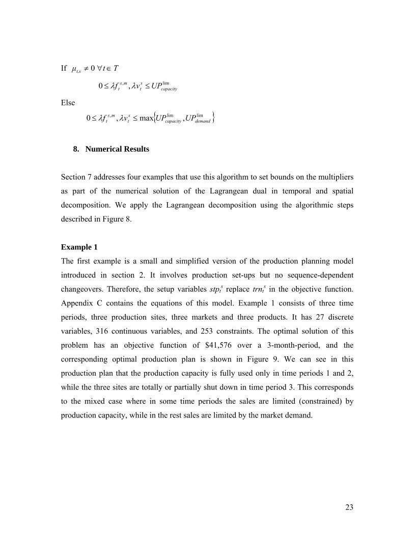
If Tt μt,s 0
lim, ,0 capacityst
mst UPvf
Else
limlim, ,max,0 demandcapacityst
mst UPUPvf
8. Numerical Results
Section 7 addresses four examples that use this algorithm to set bounds on the multipliers
as part of the numerical solution of the Lagrangean dual in temporal and spatial
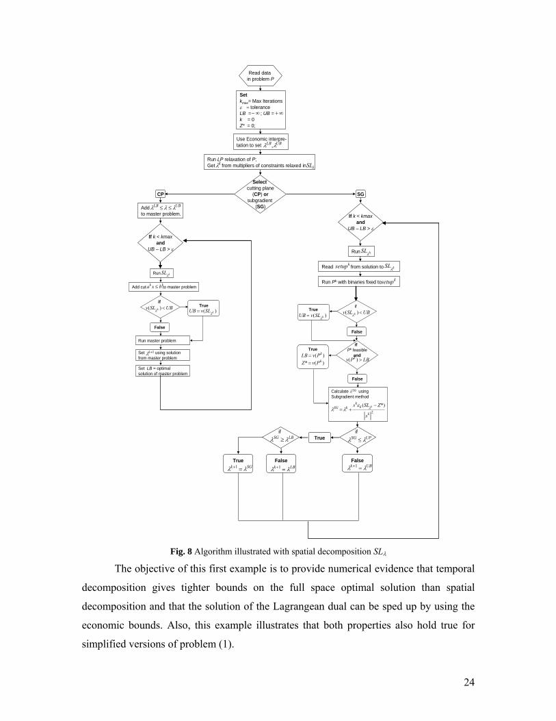
decomposition. We apply the Lagrangean decomposition using the algorithmic steps
described in Figure 8.
Example 1
The first example is a small and simplified version of the production planning model
introduced in section 2. It involves production set-ups but no sequence-dependent
changeovers. Therefore, the setup variables stpts replace trnt
s in the objective function.
Appendix C contains the equations of this model. Example 1 consists of three time
periods, three production sites, three markets and three products. It has 27 discrete
variables, 316 continuous variables, and 253 constraints. The optimal solution of this
problem has an objective function of $41,576 over a 3-month-period, and the
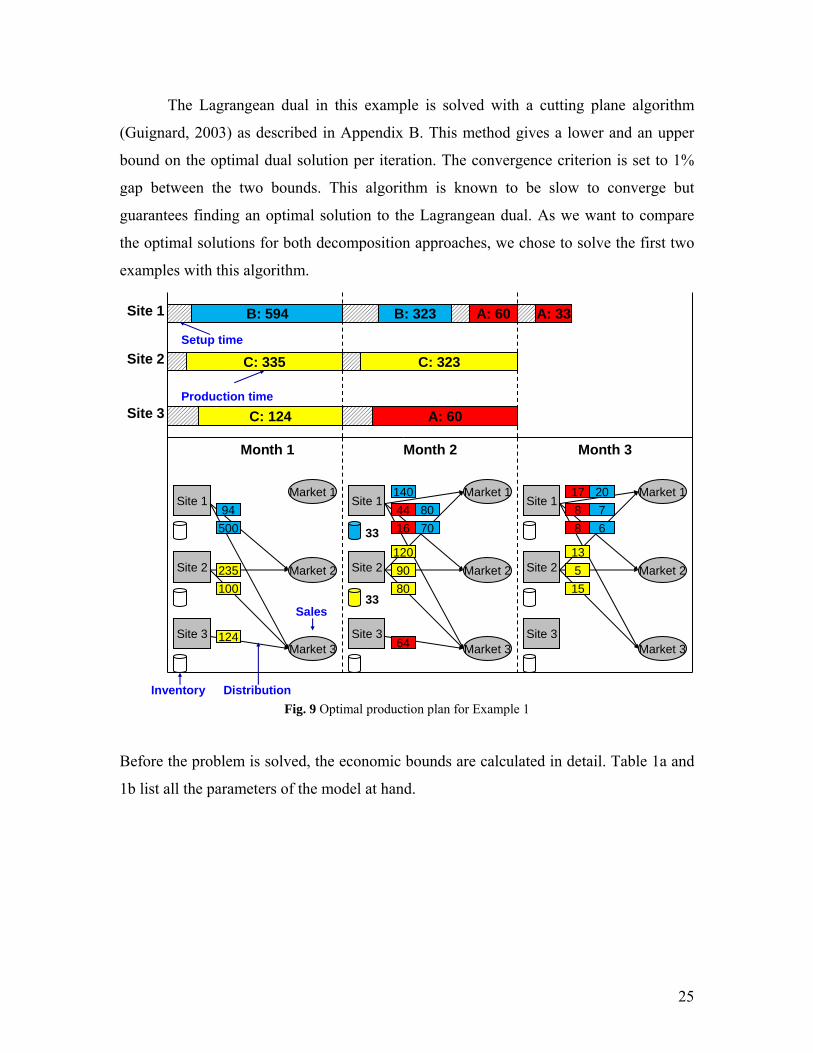
corresponding optimal production plan is shown in Figure 9. We can see in this
production plan that the production capacity is fully used only in time periods 1 and 2,
while the three sites are totally or partially shut down in time period 3. This corresponds
to the mixed case where in some time periods the sales are limited (constrained) by
production capacity, while in the rest sales are limited by the market demand.
24
Fig. 8 Algorithm illustrated with spatial decomposition SL
The objective of this first example is to provide numerical evidence that temporal
decomposition gives tighter bounds on the full space optimal solution than spatial
decomposition and that the solution of the Lagrangean dual can be sped up by using the
economic bounds. Also, this example illustrates that both properties also hold true for
simplified versions of problem (1).
Setkmax= Max Iterations toleranceLB = ; UB =k = 0Z* = 0;
Selectcutting plane
(CP) orsubgradient
(SG)
CP
If k < kmaxand
UB – LB >
Use Economic interpre-tation to set
Read data in problem P
UBLB ,
Run LP relaxation of P;Get from multipliers of constraints relaxed in k SL
Addto master problem.
UBLB
SG
If k < kmaxand
UB – LB >
Run kSL
Read from solution to kSLksetup
Run Pk with binaries fixed to ksetup
Run kSL
Add cut to master problem kk bxa
Run master problem
Set using solution from master problem
1k
Set LB = optimal solution of master problem
ifUBSLv k )(
True)( kSLvUB
False
if UBSLv k )(
True)( kSLvUB
False
if Pk feasible
andLBPv k )(
True
)( kPvLB
False
Calculate SG using Subgradient method
2
*)(
k
kk
kSG
s
ZSLs k
)(* kPvZ
if UPSG
False
if LBSG True
LBk 1
TrueSGk 1
FalseUBk 1
s
25
The Lagrangean dual in this example is solved with a cutting plane algorithm
(Guignard, 2003) as described in Appendix B. This method gives a lower and an upper
bound on the optimal dual solution per iteration. The convergence criterion is set to 1%
gap between the two bounds. This algorithm is known to be slow to converge but
guarantees finding an optimal solution to the Lagrangean dual. As we want to compare
the optimal solutions for both decomposition approaches, we chose to solve the first two
examples with this algorithm.
Fig. 9 Optimal production plan for Example 1
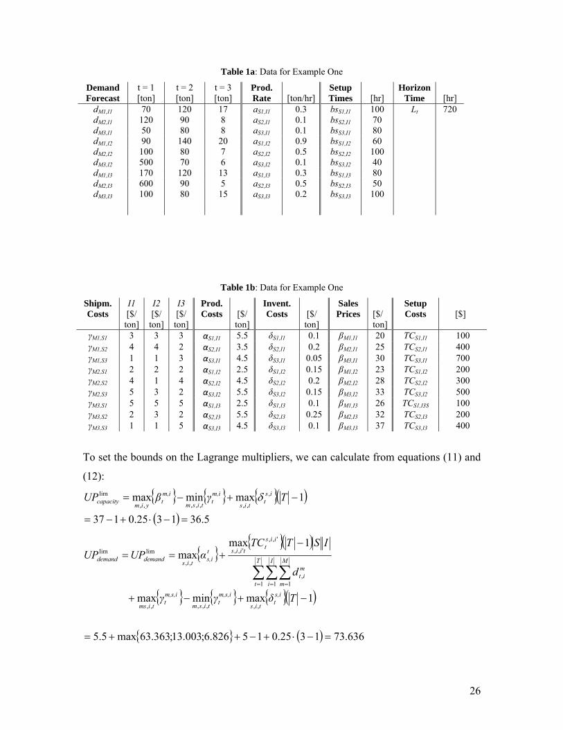
Before the problem is solved, the economic bounds are calculated in detail. Table 1a and
1b list all the parameters of the model at hand.
C: 124
B: 594Site 1
Site 1Market 1
33
Month 1 Month 2
Setup time
Inventory
Sales
Market 2
Market 3
Site 2
Site 3
Distribution
Month 3
C: 335
B: 323 A: 60
C: 323
A: 60
A: 33
Production time
Site 2
Site 3
Site 1Market 1
Market 2
Market 3
140
Site 2
Site 3
Site 1Market 1
Market 2
Market 3
17
Site 2
Site 3
33
20
120 13
44 894 80 7
235 90 5
124
16 8500 70 6
100 80 15
64
26
Table 1a: Data for Example One
Demand Forecast
t = 1 [ton]
t = 2 [ton]
t = 3 [ton]
Prod. Rate
[ton/hr]
Setup Times
[hr]
Horizon Time
[hr]
dM1,I1 70 120 17 aS1,I1 0.3 bsS1,I1 100 Lt 720 dM2,I1 120 90 8 aS2,I1 0.1 bsS2,I1 70 dM3,I1 50 80 8 aS3,I1 0.1 bsS3,I1 80 dM1,I2 90 140 20 aS1,I2 0.9 bsS1,I2 60 dM2,I2 100 80 7 aS2,I2 0.5 bsS2,I2 100 dM3,I2 500 70 6 aS3,I2 0.1 bsS3,I2 40 dM1,I3 170 120 13 aS1,I3 0.3 bsS1,I3 80 dM2,I3 600 90 5 aS2,I3 0.5 bsS2,I3 50 dM3,I3 100 80 15 aS3,I3 0.2 bsS3,I3 100
Table 1b: Data for Example One
Shipm. Costs
I1
[$/ ton]
I2 [$/ ton]
I3 [$/ ton]
Prod. Costs
[$/ ton]
Invent. Costs
[$/ ton]
Sales Prices
[$/ ton]
Setup Costs
[$]
γM1,S1 3 3 3 αS1,I1 5.5 δS1,I1 0.1 βM1,I1 20 TCS1,I1 100 γM1,S2 4 4 2 αS2,I1 3.5 δS2,I1 0.2 βM2,I1 25 TCS2,I1 400 γM1,S3 1 1 3 αS3,I1 4.5 δS3,I1 0.05 βM3,I1 30 TCS3,I1 700 γM2,S1 2 2 2 αS1,I2 2.5 δS1,I2 0.15 βM1,I2 23 TCS1,I2 200 γM2,S2 4 1 4 αS2,I2 4.5 δS2,I2 0.2 βM2,I2 28 TCS2,I2 300 γM2,S3 5 3 2 αS3,I2 5.5 δS3,I2 0.15 βM3,I2 33 TCS3,I2 500 γM3,S1 5 5 5 αS1,I3 2.5 δS1,I3 0.1 βM1,I3 26 TCS1,I3$ 100 γM3,S2 2 3 2 αS2,I3 5.5 δS2,I3 0.25 βM2,I3 32 TCS2,I3 200 γM3,S3 1 1 5 αS3,I3 4.5 δS3,I3 0.1 βM3,I3 37 TCS3,I3 400
To set the bounds on the Lagrange multipliers, we can calculate from equations (11) and
(12):
5.361325.0137
1maxminmax ,
,,,,,,,
lim
TγβUP ist
tis
m,it
tism
m,it
yimcapacity
636.731325.015826.6;003.13;363.63max5.5
1maxminmax
1maxmax
,,,,,,,
1 1 1,
',,
',,
,,
limlim
Tδγγ
d
ISTTCαUPUP
s,it
tis
m,s,it
tism
m,s,it
tims
T
t
I
i
M
m
mit
iist
tiists,i
tisdemanddemand
27
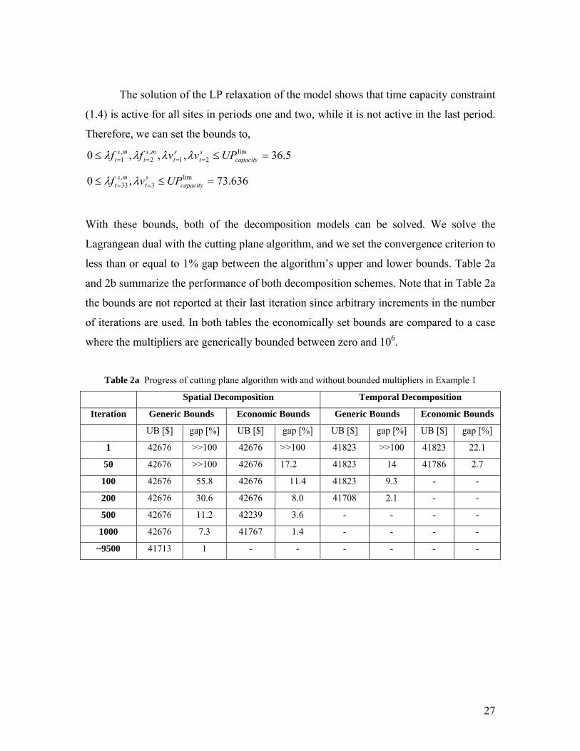
The solution of the LP relaxation of the model shows that time capacity constraint
(1.4) is active for all sites in periods one and two, while it is not active in the last period.
Therefore, we can set the bounds to,
5.36,,,0 lim21
,2
,1 capacity
st
st
mst
mst UPvvff
636.73,0 lim3
,33 capacity
st
mst UPvf
With these bounds, both of the decomposition models can be solved. We solve the
Lagrangean dual with the cutting plane algorithm, and we set the convergence criterion to
less than or equal to 1% gap between the algorithm’s upper and lower bounds. Table 2a
and 2b summarize the performance of both decomposition schemes. Note that in Table 2a
the bounds are not reported at their last iteration since arbitrary increments in the number
of iterations are used. In both tables the economically set bounds are compared to a case
where the multipliers are generically bounded between zero and 106.
Table 2a Progress of cutting plane algorithm with and without bounded multipliers in Example 1
Spatial Decomposition Temporal Decomposition
Iteration Generic Bounds Economic Bounds Generic Bounds Economic Bounds
UB [$] gap [%] UB [$] gap [%] UB [$] gap [%] UB [$] gap [%]
1 42676 >>100 42676 >>100 41823 >>100 41823 22.1
50 42676 >>100 42676 17.2 41823 14 41786 2.7
100 42676 55.8 42676 11.4 41823 9.3 - -
200 42676 30.6 42676 8.0 41708 2.1 - -
500 42676 11.2 42239 3.6 - - - -
1000 42676 7.3 41767 1.4 - - - -
~9500 41713 1 - - - - - -
28
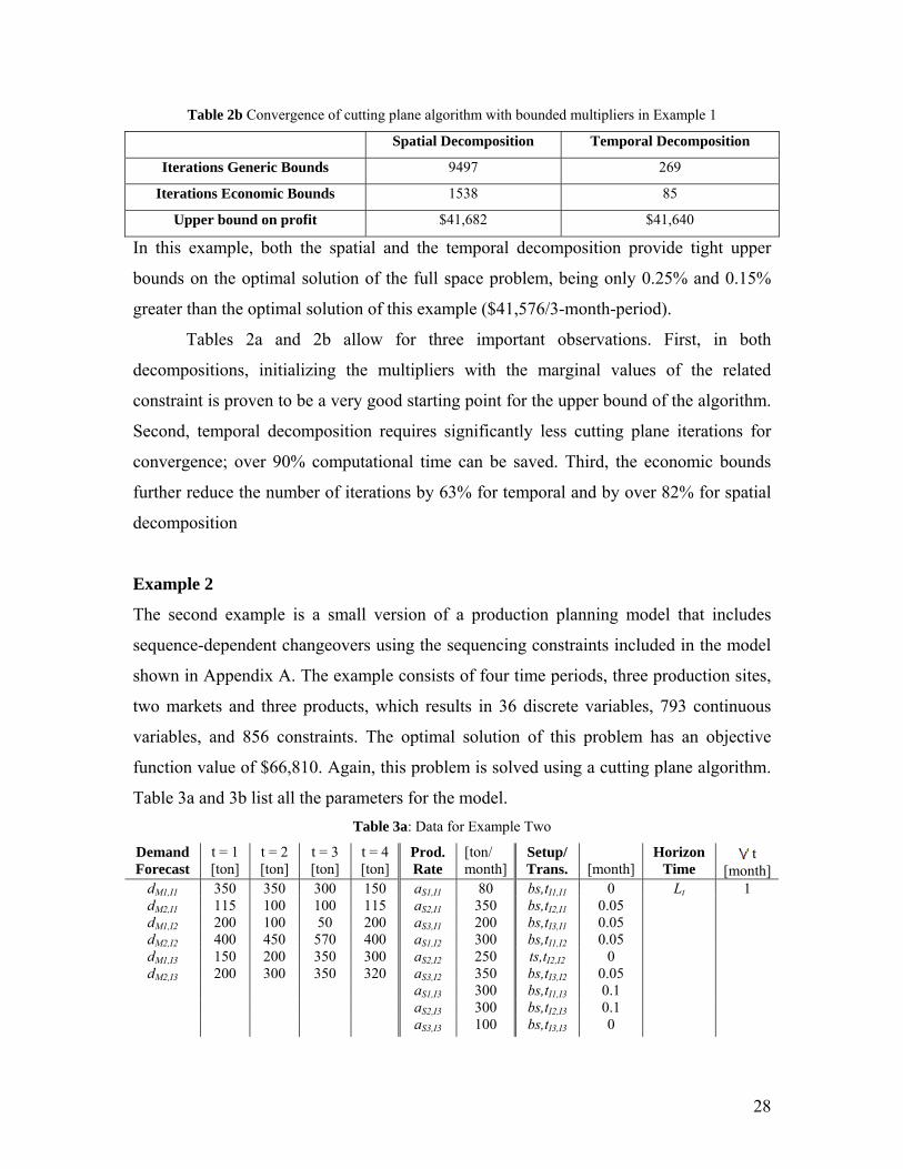
Table 2b Convergence of cutting plane algorithm with bounded multipliers in Example 1
Spatial Decomposition Temporal Decomposition
Iterations Generic Bounds 9497 269
Iterations Economic Bounds 1538 85
Upper bound on profit $41,682 $41,640
In this example, both the spatial and the temporal decomposition provide tight upper
bounds on the optimal solution of the full space problem, being only 0.25% and 0.15%
greater than the optimal solution of this example ($41,576/3-month-period).
Tables 2a and 2b allow for three important observations. First, in both
decompositions, initializing the multipliers with the marginal values of the related
constraint is proven to be a very good starting point for the upper bound of the algorithm.
Second, temporal decomposition requires significantly less cutting plane iterations for
convergence; over 90% computational time can be saved. Third, the economic bounds
further reduce the number of iterations by 63% for temporal and by over 82% for spatial
decomposition
Example 2
The second example is a small version of a production planning model that includes
sequence-dependent changeovers using the sequencing constraints included in the model
shown in Appendix A. The example consists of four time periods, three production sites,
two markets and three products, which results in 36 discrete variables, 793 continuous
variables, and 856 constraints. The optimal solution of this problem has an objective
function value of $66,810. Again, this problem is solved using a cutting plane algorithm.
Table 3a and 3b list all the parameters for the model.
Table 3a: Data for Example Two
Demand Forecast
t = 1 [ton]
t = 2 [ton]
t = 3 [ton]
t = 4 [ton]
Prod. Rate
[ton/ month]
Setup/ Trans.
[month]
Horizon Time
t [month]
dM1,I1 350 350 300 150 aS1,I1 80 bs,tI1,I1 0 Lt 1 dM2,I1 115 100 100 115 aS2,I1 350 bs,tI2,I1 0.05 dM1,I2 200 100 50 200 aS3,I1 200 bs,tI3,I1 0.05 dM2,I2 400 450 570 400 aS1,I2 300 bs,tI1,I2 0.05 dM1,I3 150 200 350 300 aS2,I2 250 ts,tI2,I2 0 dM2,I3 200 300 350 320 aS3,I2 350 bs,tI3,I2 0.05
aS1,I3 300 bs,tI1,I3 0.1 aS2,I3 300 bs,tI2,I3 0.1 aS3,I3 100 bs,tI3,I3 0
29
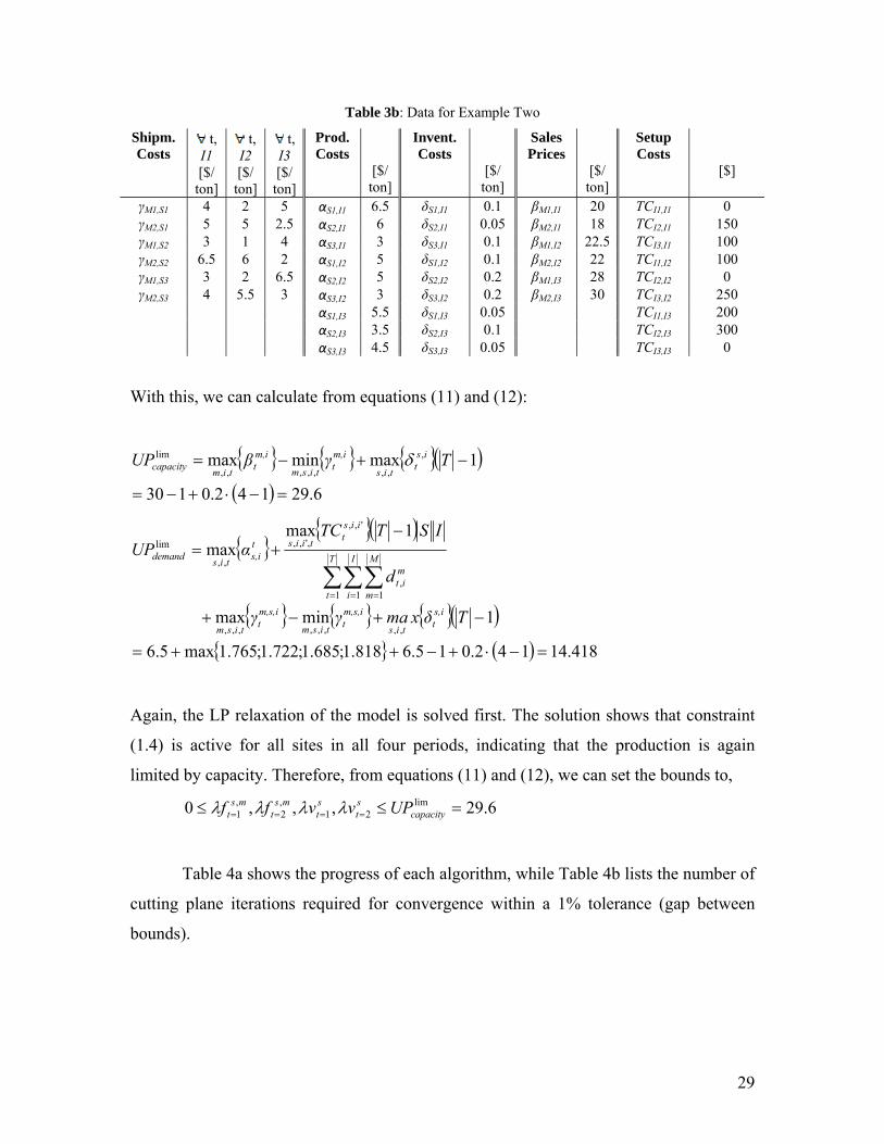
Table 3b: Data for Example Two
Shipm. Costs
t, I1 [$/ ton]
t, I2 [$/ ton]
t, I3 [$/ ton]
Prod. Costs
[$/ ton]
Invent. Costs
[$/ ton]
Sales Prices
[$/ ton]
Setup Costs
[$]
γM1,S1 4 2 5 αS1,I1 6.5 δS1,I1 0.1 βM1,I1 20 TCI1,I1 0 γM2,S1 5 5 2.5 αS2,I1 6 δS2,I1 0.05 βM2,I1 18 TCI2,I1 150 γM1,S2 3 1 4 αS3,I1 3 δS3,I1 0.1 βM1,I2 22.5 TCI3,I1 100 γM2,S2 6.5 6 2 αS1,I2 5 δS1,I2 0.1 βM2,I2 22 TCI1,I2 100 γM1,S3 3 2 6.5 αS2,I2 5 δS2,I2 0.2 βM1,I3 28 TCI2,I2 0 γM2,S3 4 5.5 3 αS3,I2 3 δS3,I2 0.2 βM2,I3 30 TCI3,I2 250
αS1,I3 5.5 δS1,I3 0.05 TCI1,I3 200 αS2,I3 3.5 δS2,I3 0.1 TCI2,I3 300 αS3,I3 4.5 δS3,I3 0.05 TCI3,I3 0
With this, we can calculate from equations (11) and (12):
6.29142.0130
1maxminmax ,
,,,,,,,
lim
TγβUP ist
tis
m,it
tism
m,it
timcapacity
418.14142.015.6818.1;685.1;722.1;765.1max5.6
1minmax
1maxmax
,,,,,,,,
1 1 1,
',,
,',,
,,
lim
Tδxmaγγ
d
ISTTCαUP
s,it
tis
m,s,it
tism
m,s,it
tism
T
t
I
i
M
m
mit
iist
tiists,i
tisdemand
Again, the LP relaxation of the model is solved first. The solution shows that constraint
(1.4) is active for all sites in all four periods, indicating that the production is again
limited by capacity. Therefore, from equations (11) and (12), we can set the bounds to,
6.29,,,0 lim21
,2
,1 capacity
st
st
mst
mst UPvvff
Table 4a shows the progress of each algorithm, while Table 4b lists the number of
cutting plane iterations required for convergence within a 1% tolerance (gap between
bounds).

30
Table 4a Progress of cutting plane algorithm with and without bounded multipliers in Example 2
Spatial Decomposition Temporal Decomposition
Iteration Generic Bounds Economic Bounds Generic Bounds Economic Bounds
UB [$] gap [%] UB [$] gap [%] UB [$] gap [%] UB [$] gap [%]
1 67513 >>10000 67513 153 67689 >>10000 67689 166.7
50 67513 >>10000 67513 10.1 67689 41.1 67689 16.9
100 67513 76.6 67513 6.3 67689 14.6 67689 6.0
200 67513 18.3 67513 2.1 67689 5.1 67689 2.5
500 67513 7.9 67513 1.3 67600 1.4 - -
1000 67513 4.2 67319 - - - - -
10000 - - - - - - - -
Table 4b Convergence of cutting plane algorithm with bounded multipliers in Example 2
Spatial Decomposition Temporal Decomposition
Iterations Generic Bounds 2725 573
Iterations Economic Bounds 1308 363
Upper bound on profit $ 66957 $ 66945
The optimal bounds provided by spatial and temporal decomposition were very similar in
this example and within 0.22 % and 0.20 % of global optimality ($66,810/4-month-
period) respectively.
Table 4 reinforces the two observations made in the first example. Temporal
decomposition achieves savings of over 70% of the iterations needed to reach
convergence. Furthermore, the economic bounds further reduce the numbers of iterations
by over 35 % for temporal and by over 50% for spatial decomposition.
Example 3
This example is included with the objective of testing the effectiveness of both
decomposition techniques relative to the full space solution of the MILP planning
problem. The problem consists of six production sites, six markets, six products, and six
time periods. If the six products are thought of as families of products, then the problem
31
can be said to be a realistic representation of a small manufacturing network. The MILP
formulation consists of 216 discrete variables, 7,957 continuous variables, and 6,985
constraints. The problem size is moderate, but the constraints used to model sequence-
dependent changeovers make its solution computationally challenging. The sequencing
constraints correspond to those in the single-site aggregate planning model by Erdirik-
Dogan & Grossmann (2008), and are shown in the Appendix A. The sequencing model is
based on the traveling salesman problem, which is known to be NP-hard.
We solve the temporal and spatial duals using the subgradient algorithm, as
presented in Appendix B and illustrated in Figure 8. The tunable parameter k is set to
0.1. We initialize the Lagrange multipliers by solving the LP relaxation of the full space
problem and assigning the optimal dual variables of constraints (1.14), (1.15) and (1.16)
to v , tr , and f . The subgradient algorithm requires an estimate of the optimal dual
solution. We propose two alternatives to obtain this estimate. The first alternative is to
run the full space model using an efficient MILP solver, like CPLEX, to generate a
feasible solution. This strategy is useful when good feasible solutions are available early
on the Branch and Bound algorithm. For this reason we set a short time limit for this
initialization step. The second alternative can be used when the full space model is too
large and/or a feasible solution is not available in a reasonable time. If this is the case, we
propose to use a simple heuristic that consists in fixing the value of the binary variables
to those obtained in the solution to the Lagrangean subproblems, TL in temporal
decomposition, or SL in the spatial decomposition. There is no guarantee that the
solution will be feasible, although in our calculations we were always able to construct a
feasible solution in this way. Since the subgradient is an iterative algorithm, we solve
TL or SL , and we construct a heuristic solution in every iteration. The solution to the
Lagrangean subproblem is an upper bound, and the heuristic solution is a lower bound
that is also used for estimating the optimal dual solution in the subgradient algorithm.
The upper and lower bounds are only updated in iterations were there is improvement,
i.e., when we find tighter bounds.
We solve the temporally and spatially decomposed problems with and without the
economic bounds for the multipliers. The problem is set up in a way that monthly market
32
demand is sometimes greater and sometimes smaller than production capacity. Therefore,
there is incentive to overproduce and build up inventory in those months were there is
extra capacity. All calculations were performed using the MILP solver CPLEX 12.1 with
GAMS 23.3.3, and run using a 2.79 GHz processor on machine with 2.5 GB of RAM.
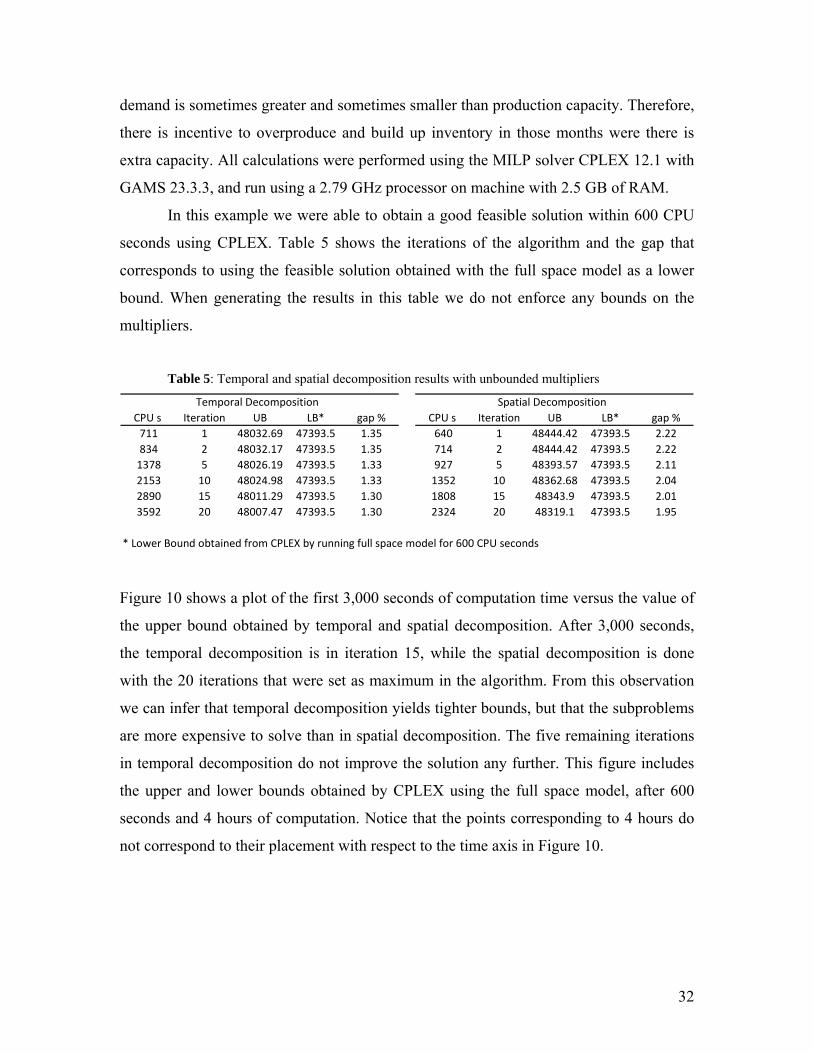
In this example we were able to obtain a good feasible solution within 600 CPU
seconds using CPLEX. Table 5 shows the iterations of the algorithm and the gap that
corresponds to using the feasible solution obtained with the full space model as a lower
bound. When generating the results in this table we do not enforce any bounds on the
multipliers.
Table 5: Temporal and spatial decomposition results with unbounded multipliers
CPU s Iteration UB LB* gap % CPU s Iteration UB LB* gap %
711 1 48032.69 47393.5 1.35 640 1 48444.42 47393.5 2.22
834 2 48032.17 47393.5 1.35 714 2 48444.42 47393.5 2.22
1378 5 48026.19 47393.5 1.33 927 5 48393.57 47393.5 2.11
2153 10 48024.98 47393.5 1.33 1352 10 48362.68 47393.5 2.04
2890 15 48011.29 47393.5 1.30 1808 15 48343.9 47393.5 2.01
3592 20 48007.47 47393.5 1.30 2324 20 48319.1 47393.5 1.95
* Lower Bound obtained from CPLEX by running full space model for 600 CPU seconds
Temporal Decomposition Spatial Decomposition
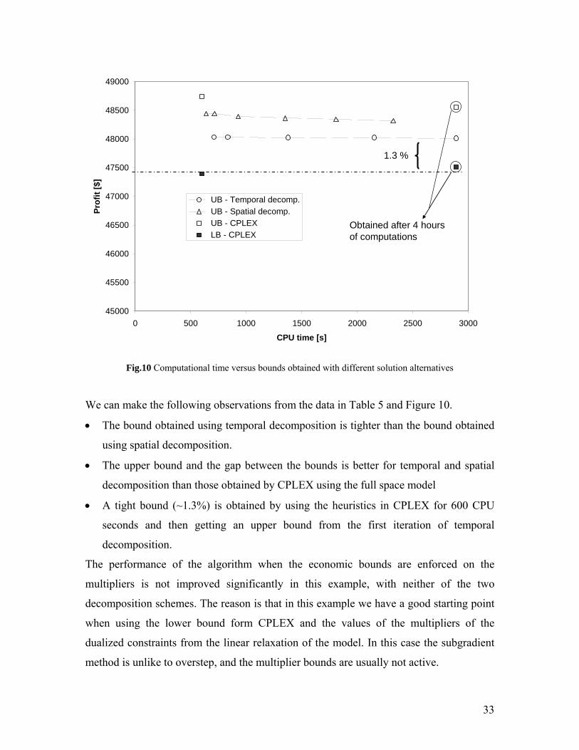
Figure 10 shows a plot of the first 3,000 seconds of computation time versus the value of
the upper bound obtained by temporal and spatial decomposition. After 3,000 seconds,
the temporal decomposition is in iteration 15, while the spatial decomposition is done
with the 20 iterations that were set as maximum in the algorithm. From this observation
we can infer that temporal decomposition yields tighter bounds, but that the subproblems
are more expensive to solve than in spatial decomposition. The five remaining iterations
in temporal decomposition do not improve the solution any further. This figure includes
the upper and lower bounds obtained by CPLEX using the full space model, after 600
seconds and 4 hours of computation. Notice that the points corresponding to 4 hours do
not correspond to their placement with respect to the time axis in Figure 10.
33
Fig.10 Computational time versus bounds obtained with different solution alternatives
We can make the following observations from the data in Table 5 and Figure 10.
The bound obtained using temporal decomposition is tighter than the bound obtained
using spatial decomposition.
The upper bound and the gap between the bounds is better for temporal and spatial
decomposition than those obtained by CPLEX using the full space model
A tight bound (~1.3%) is obtained by using the heuristics in CPLEX for 600 CPU
seconds and then getting an upper bound from the first iteration of temporal
decomposition.
The performance of the algorithm when the economic bounds are enforced on the
multipliers is not improved significantly in this example, with neither of the two
decomposition schemes. The reason is that in this example we have a good starting point
when using the lower bound form CPLEX and the values of the multipliers of the
dualized constraints from the linear relaxation of the model. In this case the subgradient
method is unlike to overstep, and the multiplier bounds are usually not active.
45000
45500
46000
46500
47000
47500
48000
48500
49000
0 500 1000 1500 2000 2500 3000
CPU time [s]
Pro
fit
[$]
UB - Temporal decomp.
UB - Spatial decomp.UB - CPLEXLB - CPLEX
1.3 %
Obtained after 4 hours of computations
34
Example 4
The last example is included in order to test the efficiency of our algorithm with a larger
problem. This instance of the planning problem includes 20 products, 10 markets, 6
production sites, and 6 time periods. The resulting MILP has 720 discrete variables,
68,437 continuous variables, and 52,381 constraints. Example 4 is handled in the same
way as Example 3 with regards to the tunable parameter k and to the initialization of the
Lagrange multipliers. In this example we cannot obtain a feasible solution from CPLEX
in a short enough time (it takes as much as running several iterations of the
decomposition algorithm) so we construct feasible solutions by the second alternative
described in Example 3. That is, we fix the value of the binary variables to those obtained
in the solution to Lagrangean sub problems, TL in temporal decomposition, or SL in
spatial decomposition.
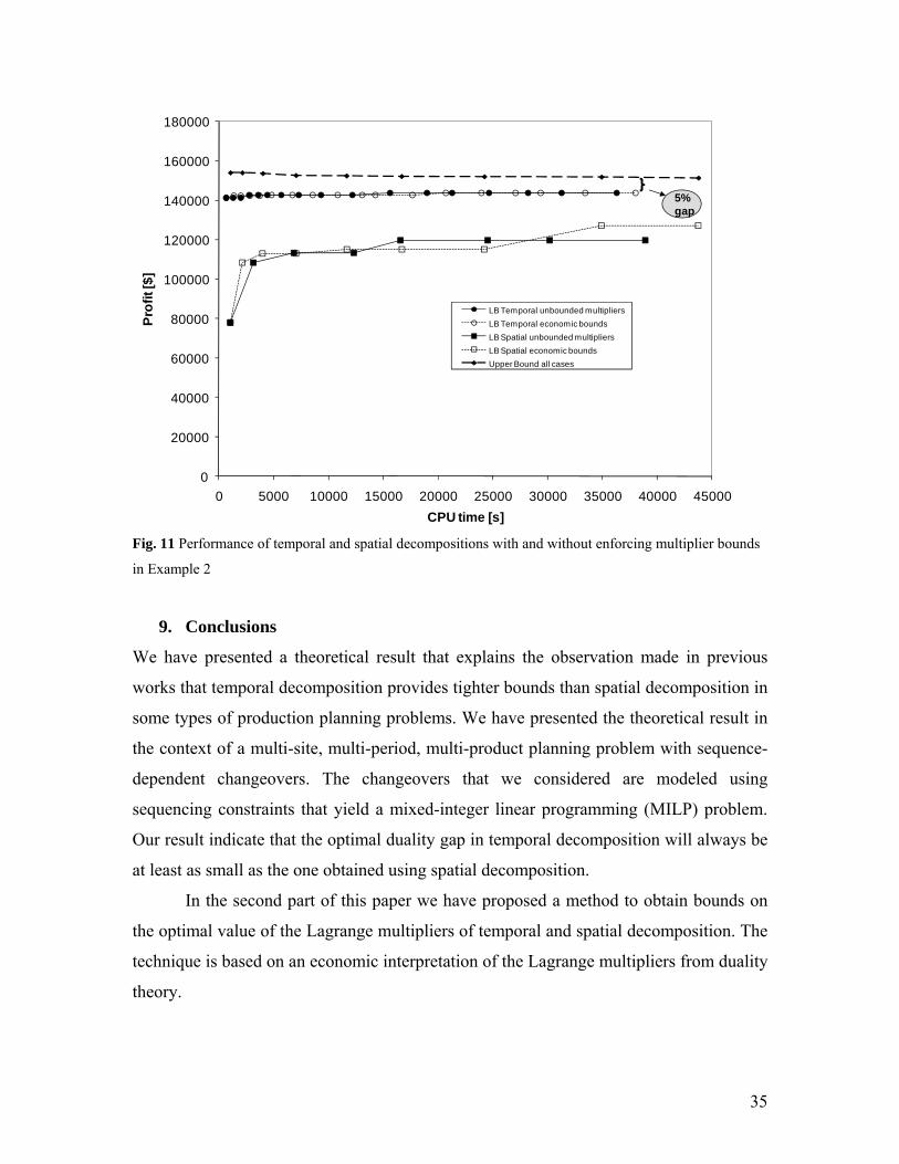
The results are summarized in Figure 11, where it can be seen that temporal
decomposition provides tighter bounds in shorter computation time. No significant
improvement is reported for the temporal decomposition when the economic bounds are
enforced. In contrast the progress of the algorithm using spatial decomposition was
enhanced by bounding the multipliers. We think that since spatial decomposition has a
looser relaxation, the beneficial effect of bounding the multipliers has a more significant
effect than in temporal decomposition. Also, we do not derive any bounds on the
multipliers of constraint (1.14), which are involved in temporal decomposition, whereas
we derive bounds for all the multipliers in spatial decomposition.
35
s
0
20000
40000
60000
80000
100000
120000
140000
160000
180000
0 5000 10000 15000 20000 25000 30000 35000 40000 45000
Pro
fit [
$]
CPU time [s]
LB Temporal unbounded multipliers
LB Temporal economic bounds
LB Spatial unbounded multipliers
LB Spatial economic bounds
Upper Bound all cases
5%gap
Fig. 11 Performance of temporal and spatial decompositions with and without enforcing multiplier bounds
in Example 2
9. Conclusions
We have presented a theoretical result that explains the observation made in previous
works that temporal decomposition provides tighter bounds than spatial decomposition in
some types of production planning problems. We have presented the theoretical result in
the context of a multi-site, multi-period, multi-product planning problem with sequence-
dependent changeovers. The changeovers that we considered are modeled using
sequencing constraints that yield a mixed-integer linear programming (MILP) problem.
Our result indicate that the optimal duality gap in temporal decomposition will always be
at least as small as the one obtained using spatial decomposition.
In the second part of this paper we have proposed a method to obtain bounds on
the optimal value of the Lagrange multipliers of temporal and spatial decomposition. The
technique is based on an economic interpretation of the Lagrange multipliers from duality
theory.
36
We have presented numerical results for four examples. The first two are used to
give some numerical evidence that the optimal solution of the temporal dual is at least as
tight as in the spatial dual. The cutting plane algorithm was used to solve these two
examples. Applying the economic bounds on the multipliers speeds the convergence of
this algorithm, particularly when solving the spatial dual. The third and fourth examples
consist of larger planning problems and were solved using the subgradient method. The
results indicate that the decomposition strategies are efficient for larger problems, and
that the bound provided by temporal decomposition was confirmed to be tighter than the
bound from spatial decomposition. The economic bounds enhanced the convergence of
spatial decomposition in larger problems with loose initial bounds.
Acknowledgments
The authors would like to acknowledge financial support by the Dow Chemical Company
for this project.
References Chen P. and J. M. Pinto (2008). Lagrangean-based techniques for the supply chain
management of flexible process networks. Computers and Chemical Engineering, 32, 2505 – 2528.
Chvátal V., Linear Programming. W. H. Freeman and Company, New York (1983). Dorfman R., P. A. Samuelson and R. M. Solow, Linear Programming and Economic
Analysis. McGraw Hill Book Company, New York (1958). Erdirik-Dogan M. and I. E. Grossmann (2008). Simultaneous planning and scheduling of
single-stage multiproduct continuous plants with parallel lines. Computers and Chemical Engineering, 32, 2664 – 2683.
Guignard M. (2003). Lagrangean Relaxation. Top, 11(2), 151 – 228 . Geoffrion A. M. (1974). Lagrangean Relaxation for Integer Programming. Mathematical
Programming Study, 2, 82 – 114. Gupta A. and C. D. Maranas (1999). A Hierarchical Lagrangean Relaxation Procedure
for Solving Midterm Planning Problems. Industrial and Engineering Chemistry Research, 38, 1937 – 1947.
37
Jackson J. R. and I. E. Grossmann (2003). Temporal Decomposition Scheme for Nonlinear-Multisite Production Planning and Distribution Models. Industrial and Engineering Chemistry Research, 42(13), 3045 – 3055.
Neiro S.M.S. and J. M. Pinto (2006). Lagrangean decomposition applied to multiperiod
planning of petroleum refineries under uncertainty. Latin American Applied Research, 36, 213 – 220.
Pochet Y. and L. A. Wolsey. Production Planning by Mixed Integer Programming.
Springer, New York (2006). Trotter P. A.,(2009). Economic Interpretation of Lagrange Multipliers in Lagrangean
Decomposition of a Planning Problem , Technical Report, RWTH Aachen University. Williams H. P. (1996). Duality in Mathematics and Linear and Integer Programming.
Journal of Optimization Theory and Applications, 90(2), 257 – 278. Wu D. and M. Ierapetritou (2006). Lagrangean decomposition using an improved Nelder-
Mead approach for Lagrangean multiplier update. Computers and Chemical Engineering, 30, 778 – 789.
Appendix A
Production planning model
The model presented in this appendix is an extension of the MILP model by Erdirik-
Dogan and Grossmann (2008) for the case of multi-site production of continuous multi-
product plants with parallel lines.
Nomenclature
Index/Set
i,k/I indices/set of products
s/S index/set of manufacturing sites
t/T index/set of time periods
m/M index/set of markets
Parameters
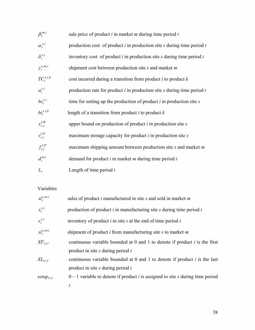
38
imt
, sale price of product i in market m during time period t
ist
, production cost of product i in production site s during time period t
ist
, inventory cost of product i in production site s during time period t
imst
,, shipment cost between production site s and market m
kistTC ,, cost incurred during a transition from product i to product k
ista , production rate for product i in production site s during time period t
istbs , time for setting up the production of product i in production site s
kistbt ,, length of a transition from product i to product k
UBisx , upper bound on production of product i in production site s
UPisv , maximum storage capacity for product i in production site s
UPisf , maximum shipping amount between production site s and market m
imtd , demand for product i in market m during time period t
tL Length of time period t
Variables
imstsl ,, sales of product i manufactured in site s and sold in market m
istx , production of product i in manufacturing site s during time period t
istv , inventory of product i in site s at the end of time period t
imstsl ,, shipment of product i from manufacturing site s to market m
XFi,s,t continuous variable bounded at 0 and 1 to denote if product i is the first
product in site s during period t
XLi,s,t continuous variable bounded at 0 and 1 to denote if product i is the last
product in site s during period i
setupi,s,t 0 – 1 variable to denote if product i is assigned to site s during time period
t
39
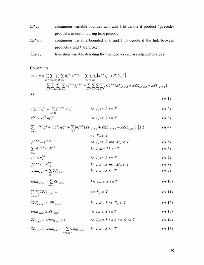
ZPi,k,s,t continuous variable bounded at 0 and 1 to denote if product i precedes
product k in unit m during time period t
ZZPi,k,s,t continuous variable bounded at 0 and 1 to denote if the link between
products i and k are broken
ZZZi,k,s,t transition variable denoting the changeovers across adjacent periods
Constraints
..
)(
max
,,,,,,,,,,,,,,,
,,,,,,,
ts
ZZPZZZZPTCf
vxsl
Tt Ss Ii Iktmkitmkitmki
kist
Tt Ss Mm Ii
imst
imst
Tt ss Ii
ist
ist
ist
ist
Tt Ss Mm Ii
imst
imt
(A.1)
ist
Mm
imst
ist
ist vfxv ,,,,,
1
TtSsIi ,, (A.2)
ist
UBis
ist stpxx ,
,, TtSsIi ,, (A.3)
LZZPZZZZPbtstpbsxa tIi Ik
tmkitmkitmkikis
tis
tis
tis
tis
t
)( ,,,,,,,,,
,,,,,, (A.4)
TtSs ,
s,m,it
s,m,it slf TtMmSsIi ,,, (A.5)
imt
Ss
imst dsl ,,,
TtMmIi ,, (A.6)
vv UBs,i
s,it TtSsIi ,, (A.7)
ff UBs,m,i
s,m,it TtMmSsIi ,,, (A.8)
Ik
tskitsi ZPsetup ,,,,, TtSsIi ,, (A.9)
Ik
tskitsk ZPsetup ,,,,, TtSsIk ,, (A.10)
Ii Kk
tmkiZZP 1,,, TtSs , (A.11)
tmkitmki ZPZZP ,,,,,, TtSsIkIi ,,, (A.12)
tsiitsi ZPsetup ,,,,, TtSsIi ,, (A.13)
1,,,,, tsktsii setupZP TtSskiIkIi ,,,, (A.14)
Ikik
tmktsitsii setupsetupZP,
..,,,,, TtSsIi ,, (A.15)
40
Ii
tskitsk ZZPXF ,,,,, TtSsIi ,, (A.16)
Ik
tskitsi ZZPXL ,,,,, TtSsIi ,, (A.17)
Ii
tsiXF 1,, TtSsIi ,, (A.18)
Ii
tsiXL 1,, TtSsIi ,, (A.19)
tsiIk
tski XLZZZ ,,,,,
TtSsIi ,, (A.20)
1,,,,,
tskIi
tski XFZZZ TtSsIk ,, (A.21)
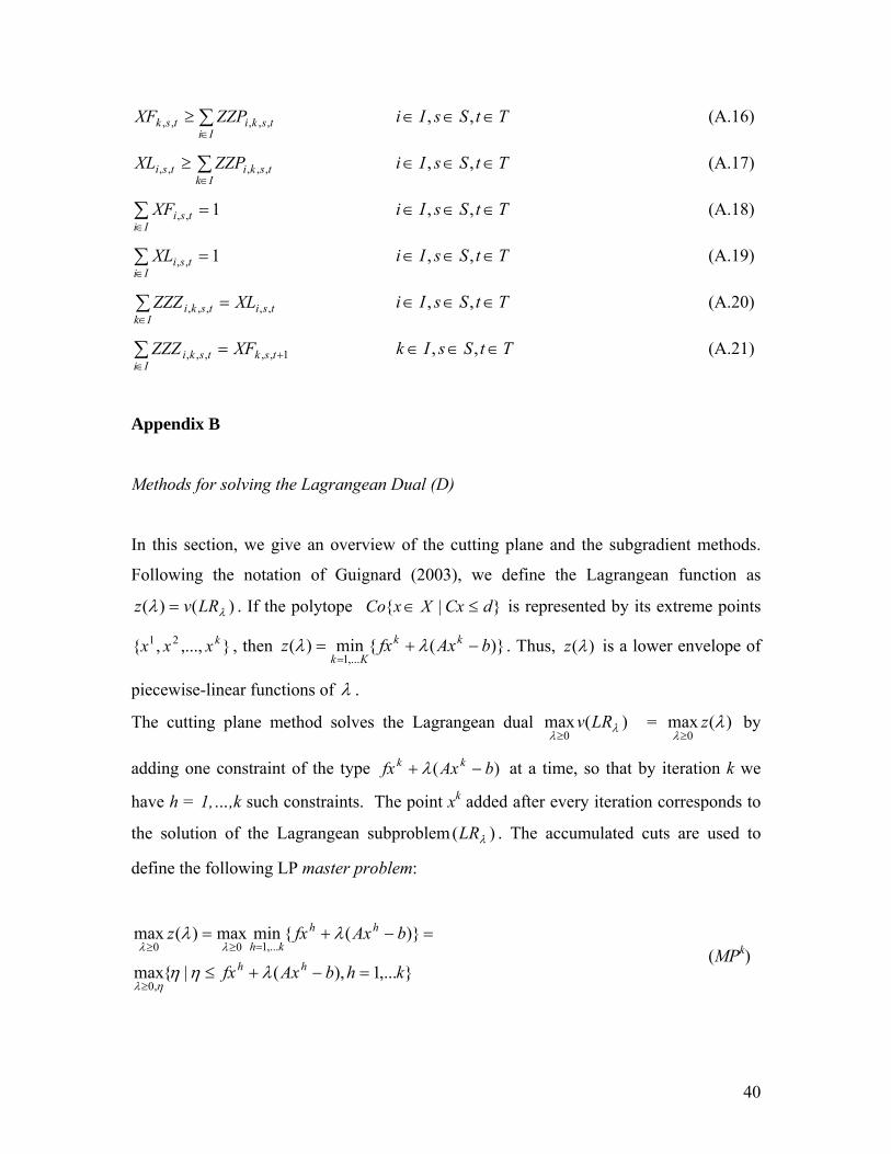
Appendix B Methods for solving the Lagrangean Dual (D)
In this section, we give an overview of the cutting plane and the subgradient methods.
Following the notation of Guignard (2003), we define the Lagrangean function as
)()( LRvz . If the polytope }|{ dCxXxCo is represented by its extreme points
},...,,{ 21 kxxx , then )}({min)(,...1
bAxfxz kk
Kk
. Thus, )(z is a lower envelope of
piecewise-linear functions of .
The cutting plane method solves the Lagrangean dual )(max0
LRv
= )(max0
z
by
adding one constraint of the type )( bAxfx kk at a time, so that by iteration k we
have h = 1,…,k such constraints. The point xk added after every iteration corresponds to
the solution of the Lagrangean subproblem )( LR . The accumulated cuts are used to
define the following LP master problem:
},...1),(|{max
)}({minmax)(max
,0
,...100
khbAxfx
bAxfxz
hh
hh
kh
(MPk)
41
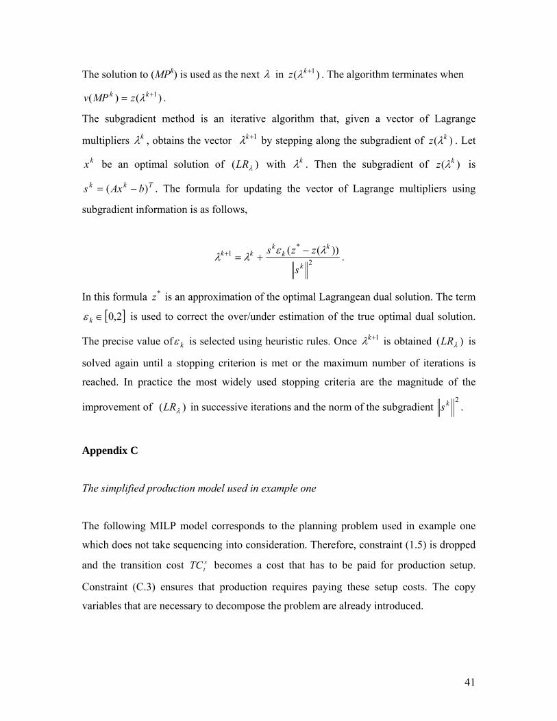
The solution to (MPk) is used as the next in )( 1kz . The algorithm terminates when
)()( 1 kk zMPv .
The subgradient method is an iterative algorithm that, given a vector of Lagrange
multipliers k , obtains the vector 1k by stepping along the subgradient of )( kz . Let
kx be an optimal solution of )( LR with k . Then the subgradient of )( kz is
Tkk bAxs )( . The formula for updating the vector of Lagrange multipliers using
subgradient information is as follows,
2
*1 ))((
k
kk
kkk
s
zzs .
In this formula *z is an approximation of the optimal Lagrangean dual solution. The term
2,0k is used to correct the over/under estimation of the true optimal dual solution.
The precise value of k is selected using heuristic rules. Once 1k is obtained )( LR is
solved again until a stopping criterion is met or the maximum number of iterations is
reached. In practice the most widely used stopping criteria are the magnitude of the
improvement of )( LR in successive iterations and the norm of the subgradient 2ks .
Appendix C
The simplified production model used in example one
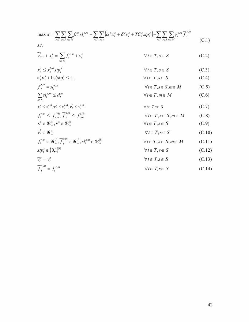
The following MILP model corresponds to the planning problem used in example one
which does not take sequencing into consideration. Therefore, constraint (1.5) is dropped
and the transition cost stTC becomes a cost that has to be paid for production setup.
Constraint (C.3) ensures that production requires paying these setup costs. The copy
variables that are necessary to decompose the problem are already introduced.
42
..
max,,,
ts
fstpTCvxslTt Ss
ms
tMm
mst
Tt ss
st
st
st
st
st
st
Tt Ss Mm
mst
mt
(C.1)
SsTtvfxv st
Mm
mst
st
st
, ,1 (C.2)
SsTt stpxx st
UBs
st , (C.3)
SsTt , Lstpbsxa tst
st
st
st (C.4)
MmSsTt slf ms,t
ms,
t ,, (C.5)
MmTt dsl mt
Ss
mst
,, (C.6)
ST,st vv,v;vxx UBs
st
UBs
st
UBs
st (C.7)
MmSsTt f f,f f UBms,
ms,
tUBms,
ms,t ,, (C.8)
SsTt , v,x |I|st
|I|st (C.9)
SsTt , v |I|st (C.10)
MmSsTt sl,f,f |I|ms,t
|I|ms,
t|I|ms,
t ,, (C.11)
SsTt stp |I|st ,1,0 (C.12)
SsT,t vv st
st (C.13)
SsT,t ff mst
ms
t ,, (C.14)