TEMPORAL AND SPATIAL CHANGES OF PRIMARY PRODUCTIVITY IN THE SEA OF MARMARA OBTAINED BY

REMOTE SENSING

A THESIS SUBMITTED TO THE GRADUATE SCHOOL OF NATURAL AND APPLIED

SCIENCES OF

MIDDLE EAST TECHNICAL UNIVERSITY

BY

DİDEM İKİS

IN PARTIAL FULFILLMENT OF THE REQUIREMENTS FOR

THE DEGREE OF MASTER OF SCIENCE IN

BIOLOGY

SEPTEMBER 2007

Approval of the Thesis

TEMPORAL AND SPATIAL CHANGES OF PRIMARY PRODUCTIVITY IN THE SEA OF MARMARA OBTAINED BY

REMOTE SENSING submitted by Didem İkis in partial fulfillment of the requirements for the degree of Master of Science in Biology Department, Middle East Technical University by, Prof. Dr. Canan Özgen __________ Dean, Graduate School of Natural and Applied Sciences Prof. Dr. Zeki Kaya __________ Head of Department, Biology Assoc. Prof. Dr. C. Can Bilgin __________ Supervisor, Biology Dept., METU Instructor Sargun Ali Tont __________ Co-Supervisor, Biology Dept., METU Examining Committee Members: Prof. Dr. Zeki Kaya (*) __________ Biology Dept., METU Assoc. Prof. Dr. C. Can Bilgin (**) __________ Biology Dept., METU Prof.Dr. Ayşen Yılmaz __________ IMS, METU Prof.Dr. Musa Doğan __________ Biology Dept., METU Assoc.Prof. Dr. Mehmet Lütfi Süzen __________ Geological Engineering Dept., METU Date: 24.09.2007

iii

I hereby declare that all information in this document has been obtained and presented in accordance with academic rules and ethical conduct. I also declare that, as required by these rules and conduct, I have fully cited and referenced all material and results that are not original to this work. Name, Last Name: Didem İkis Signature :

iv

ABSTRACT

TEMPORAL AND SPATIAL CHANGES OF PRIMARY

PRODUCTIVITY IN THE SEA OF MARMARA OBTAINED BY

REMOTE SENSING

İkis, Didem

M.Sc., Department of Biology

Supervisor: Assoc.Prof.Dr. C. Can Bilgin

Co-Supervisor: Sargun Ali Tont

September 2007, 49 Pages

Temporal and spatial variations in the Sea of Marmara based on

monthly averages of chlorophyll a, which is the major indicator of

phytoplankton biomass and primary production, recorded by

SeaWiFS and MODIS-Aqua sensors at nearly 100 stations have

been analyzed for the period of 1997-2007. Majority of phytoplankton

blooms occur during the winter and spring seasons, followed by a

smaller secondary bloom during the fall season. The majority of high

magnitude blooms occur at the Eastern part of the Sea which may be

attributed to an increase in the amount of discharge of water

contaminated with nutrients originating on land where the industries

are located.

The correlations between monthly averages of sea surface

temperature (SST) and corresponding chlorophyll a values are

statistically significant (inverse) at 1% level, where r= -0.53 and the

equation of the fitted model is:

Chlorophyll a = 7.09199 – 0.215402* SST

v

This correlation is expected because a relative decrease in SST is an

indicative of upwelling and vertical mixing which are the primary

processes for the formation of phytoplankton blooms.

We have also found that monthly averages of chlorophyll a recorded

by SeaWiFS and MODIS-Aqua are nearly identical and either data

set can be used in place of the other.

Keywords: Primary Productivity, Sea of Marmara, Remote Sensing,

Chlorophyll a, SeaWiFS, MODIS-Aqua.

vi

ÖZ

MARMARA DENİZİ’ NDE BİRİNCİL ÜRETİMİN YERE VE ZAMANA

BAĞLI OLARAK DEĞİŞİMİNİN UZAKTAN ALGILAMA

YÖNTEMİYLE İZLENMESİ

İkis, Didem

Yüksek Lisans, Biyoloji Bölümü

Tez Yöneticisi: Doç.Dr. C. Can Bilgin

Ortak Tez Yöneticisi: Sargun Ali Tont

Eylül 2007, 49 Sayfa

Bu çalışmada, SeaWiFS ve MODIS-Aqua sensörleri tarafından 1997-

2007 yılları arasında toplanmış aylık klorofil a verileri kullanılmıştır.

100’ e yakın örnekleme istasyonundan alınan klorofil a değerleri

fitoplankton biyokütlesi ve birincil üretimin en önemli göstergesidir.

En kayda değer fitoplankton artışı, kış ve ilkbahar mevsiminde

gözlemlenmiştir. Bu büyük artışı, sonbaharda meydana gelen küçük

bir artış takip etmektedir. Marmara Denizi’nin doğu kıyıları, en yüksek

fitoplankton artışlarına sahne olmaktadır. Sanayi bölgelerinden

denize akan atık sular, yüksek miktarda besin tuzu içerdiğinden bu

yüksek artışların nedeni olabilir. Aylık deniz suyu sıcaklığı ve klorofil

a değerleri arasında yapılan regresyon analizi, bu iki parametrenin

ters orantılı ve %1 ölçüsünde istatistiksel olarak anlamlı olduğunu

ortaya çıkarmıştır. Bu analize uygun modeli ortaya koyan denklem

aşağıdaki gibidir (r= -0.53):

Chlorophyll a = 7.09199 – 0.215402* SST

vii

Deniz suyu sıcaklığındaki azalma denizin alt kesimindeki soğuk su

tabakasının yüzeye çıkmasının ve düşey karışımın bir işaretidir. Bu

durum da birincil üretimdeki büyük artışların nedenidir.

Bunların haricinde aylık klorofil a değerleri arasında yapılan analizler,

SeaWiFS and MODIS-Aqua sensörlerinin birbirleriyle çok uyumlu

olduğunu ve datalarının birlikte kullanılabileceğini ortaya koymuştur.

Anahtar Sözcükler: Birincil Üretim, Marmara Denizi, Uzaktan

Algılama, Klorofil a, SeaWiFS, MODIS-Aqua.

viii

This thesis is dedicated to the memory of My Father, Haşim İkis.

ix

ACKNOWLEDGEMENTS I would like to express my deepest gratitude to Sargun Ali Tont for

his invaluable guidance, critical discussions, and continued advice

throughout this study. His scientific knowledge and power of analysis

has broadened my academic vision. I feel myself very fortunate

because I have this marvelous man in my life as an advisor, a father

figure, a friend and a role model.

I would like to thank Assoc.Prof.Dr. Mehmet Lütfi Süzen for his

guidance, encouragement and criticism in preparing this thesis. I

especially value his help in solving problems related to remote

sensing. He helped me whenever I needed it.

I would also like to thank Assoc.Prof.Dr. C. Can Bilgin for his

guidance and encouragement in this study.

I would also like to express my gratitude to Prof. Dr. Ayşen Yılmaz for

her valuable suggestions.

My special thanks are extended to the people working in Ocean

Biology Discipline Processing Group (OBPG) and Turkish

Meteorological Office for making available the data used in this

study.

x

I would like to express my sincere gratitude to my mother, Gülden

İkis and my sister, Sinem İkis for their everlasting support and

encouragement. Their unwavering faith in me was most helpful

during this study.

I thank my wonderful friends Tuğçe Kancı, Bilge Bostan, Gizem

Bezirci, Utku Koçak and Berna Kızılgüneş for their moral support

throughout this study.

xi

TABLE OF CONTENTS

ABSTRACT ....................................................................................... iv

ÖZ .....................................................................................................vi

ACKNOWLEDGEMENTS.................................................................. ix

TABLE OF CONTENTS ....................................................................xi

LIST OF TABLES ............................................................................ xiii

LIST OF FIGURES.......................................................................... xiv

CHAPTERS

1. INTRODUCTION .................................................................... 1

1.1 Remote Sensing ............................................................... 3

1.2 Primary Productivity Patterns and Dynamics .................... 9

1.2.1 Limiting Factors in Primary Productivity................ 11

1.2.2 Temporal and Spatial Variations of Primary

Productivity ........................................................... 13

2. MATERIALS AND METHODS.............................................. 16

2.1 Sampling......................................................................... 17

2.2 Data Analysis .................................................................. 23

3. RESULTS AND DISCUSSION ............................................. 26

3.1 Patterns of Monthly Chlorophyll a Fluctuations ............... 30

3.2 SST and Chlorophyll a Correlations................................ 37

4. CONCLUSION AND RECOMMENDATIONS FOR

FUTURE STUDIES .............................................................. 39

REFERENCES................................................................................ 41

xii

APPENDICES ................................................................................. 48

Appendix A: Regression analysis between monthly

averages of Sea Surface Temperature

(SST) and Chlorophyll a concentration

during 1997-2007 period .................................. 48

xiii

LIST OF TABLES

Tables Table 1.1 Current Ocean-Color Sensors……………………………….6 Table 2.1 MODIS-Aqua and SeaWiFS spectral bands used in ocean color processing……………………………………...18 Table 3.1 Pearson Coefficients (r) between chlorophyll values measured at East-West Transects…………………………34 Table 3.2 Pearson Coefficients (r) between chlorophyll values measured at North-South Transects………………………35

xiv

LIST OF FIGURES

Figures Figure 1.1 The Sea of Marmara ........................................................ 2 Figure 1.2 Spectra of upwelled radiance measured just beneath the sea surface at different pigment concentrations .................................................................. 5 Figure 1.3 Examples of Diatoms, Dinoflagellates and Coccolithophores............................................................ 10 Figure 1.4 Eddy Formation in the Sea of Marmara ......................... 12 Figure 1.5 Variation in the biomass of phytoplankton by season and latitude ............................ 14 Figure 1.6 Typical seasonal variations in the abundance of sunlight, nutrients, microscopic plants, and grazers in surface waters at temperate latitudes ..... 15 Figure 2.1 Electromagnetic Spectrum ............................................. 16 Figure 2.2 Absorption Spectra of Chlorophyll a and b ..................... 17 Figure 2.3 A map of all data points in the SeaBASS bio-optical data set........................................................................... 19 Figure 2.4 Maps of the distributions of chlorophyll a Concentrations ............................................................... 20 Figure 2.5 In situ and SeaWiFS data set comparison...................... 21 Figure 2.6 In situ and MODIS-Aqua data set comparison ............... 21 Figure 2.7 Chlorophyll a concentrations for the month of April, 2003 calculated from images taken by MODIS-Aqua ............................................................. 22

xv

Figure 2.8 44 Sampling Stations for MODIS-Aqua .......................... 24 Figure 2.9 60 Sampling Stations for SeaWiFS ................................ 24 Figure 3.1 Chlorophyll contents of 3 stations calculated by using SeaWiFS and MODIS-Aqua data sets .................. 27 Figure 3.2 SeaWiFS Data Set ......................................................... 31 Figure 3.3 MODIS-Aqua Data Set ................................................... 32 Figure 3.4 Time Series of Monthly Averages of Chlorophyll a Concentration during 1997-2007 based on SeaWiFS and MODIS-Aqua data sets............................ 33 Figure 3.5 Averaged Chlorophyll a Concentration of Each Transect along East-West Direction ............................... 33 Figure 3.6 Averaged Chlorophyll a Concentration of Each Transect along North-South Direction ............................ 34 Figure 3.7 Monthly Cycles of Chlorophyll a Concentration (mg/m3) in the Sea of Marmara based on SeaWiFS data set...................................................... 36 Figure 3.8 Sea Surface Temperature (SST) during 1997-2007....... 38

1

CHAPTER 1

INTRODUCTION

In this study we present our findings about spatial and temporal

variations of chlorophyll a concentrations measured by remote

sensing in the Sea of Marmara during 1997-2007 period.

The name of the Marmara draws its origin from Greek word for

marble (marmaros). It is 280 km long from northeast to southwest

and nearly 80 km wide at its greatest width. Its area is 11,350 km2

and its average depth is about 494 m and maximum depth is 1,355

m. The Sea of Marmara is an inland sea located at the North-

Western part of Turkey. It is connected to Black Sea via the

Bosporus Strait from the North and to Aegean Sea via Dardanelles

straight from the South (Figure 1.1).

Figure 1.1 The Sea of Marmara (URL 1).

The water masses coming from both Black Sea and Mediterranean

Sea hold the basin of the Sea of Marmara. Brackish waters (22-26

ppt salinity) forming the thin surface layer, sourced by Black Sea, are

separated from subhalocline waters of Mediterranean Sea (38.5-38.6

ppt salinity) (Unluata et al., 1990; Besiktepe, 1991). Previous studies

have shown that Bosporus input (Istanbul and Black Sea load),

vertical mixing through stratification, diffusion and upwelling via eddy

formation are the main nutrient sources of the Sea of Marmara

(Besiktepe et al., 1994; Polat and Tugrul, 1995; Tugrul and Polat,

1995).

Total annual loads of total phosphorus, total nitrate and total organic

carbon entering to the Sea of Marmara, through the current

originated from the Black Sea, are 35, 64 and 77%, respectively

(Tugrul and Polat, 1995). Annual input of river originated total nitrate

and total organic compounds flowing from the Black Sea into the Sea

of Marmara are about three times those flowing from the Sea of

Marmara into the Black Sea (Polat and Tugrul, 1995). As stated by

2

3

Tugrul et al. (1995), “pollution discharges from Istanbul (40-65% of

the total anthropogenic discharges) have secondary importance for

the nutrient and organic carbon pools of the Marmara Sea; however,

the land-based chemical pollution has drastically modified the

ecosystems of coastal margins and semi-enclosed bays (e.g. Golden

Horn, Izmit and Gemlik) where water exchanges with the open sea

are limited.”

1.1 REMOTE SENSING As defined by Sabins (1997) Remote sensing is “the science of

acquiring, processing, and interpreting images, and related data,

obtained from aircraft and satellites that record the interaction

between matter and electromagnetic radiation.”

In employing remote sensing techniques there are 4 important

factors to be considered: (Everett and Simonett, 1976)

1. Spatial Resolution is the minimum distance between two

objects at which the images of the objects appear distinct and

separate.

2. Spectral Resolution shows the location and the number of the

spectral bands recorded by a satellite sensor.

3. Radiometric Resolution is the ability of quantifying the range of

electromagnetic energy detected by satellite sensor.

4. Temporal Resolution shows the frequency of detection of the

sampling area.

4

One of the first attempts to take pictures of a remote area has been

made from a balloon by French photographer Gaspard Felix

Tournachon in 1859. Even though he was only partially successful in

achieving his aim, his experiments caught the attention of the

military.

As a result the military personnel began to gather intelligence by

mounting cameras on balloons, planes and even pigeons (URL 2).

The techniques of exploring the earth’s surface from the space were

developed after the Soviet Union successfully launched Sputnik I in

1957. The ability of Sputnik I to gather remote sensing data was

limited to telemetric verification of exact locations on the earth’s

surface (URL 3).

The Coastal Zone Color Scanner (CZCS) which was launched in

1978 and continued operating until 1986 was the first sensor that

could detect variations in phytoplankton pigments (Hovis et al.,

1980). The principle behind this detection is that when the

phytoplankton biomass is high, phytoplankton containing chlorophyll

a absorbs light in blue and red regions of visible spectrum. Thus an

increase in phytoplankton concentration changes the color of the

ocean from red, blue to green (Figure 1.2). The low concentration of

phytoplankton biomass turns the ocean color into blue.

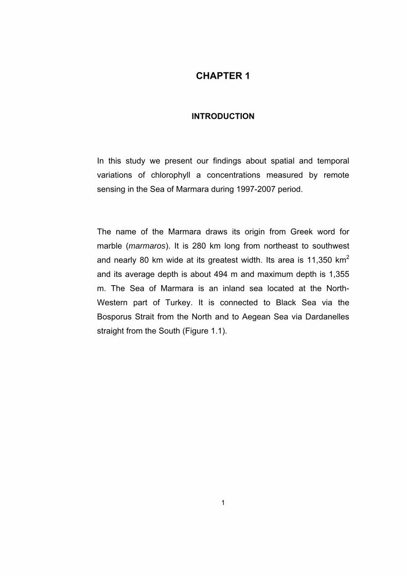
Figure 1.2 Spectra of upwelled radiance measured just beneath the

sea surface at different pigment concentrations. Spectra

corresponding to the two highest pigment concentrations were

measured in Chesapeake Bay, and the others were measured in the

Gulf of Mexico. The hatched areas represent the positions of CZCS

spectral bands 1 through 4 (Hovis et al., 1980).

The criteria explained above have been the governing principle for

the sensors launched after CZCS. 10 sensors which are currently

operating are shown in Table 1.1.

5

6

Table 1.1 Current Ocean-Color Sensors (URL 4)

Sensor Agency Satellite Launch

Date Swath (km)

Resolution (m)

Bands Spectral Coverage (nm)

Orbit

COCTS CNSA

(China)

HY-1B

(Korea)

11 Apr.

2007

1400 1100 10 402-

12,500

Polar

CZI CNSA

(China)

HY-1B

(Korea)

11 Apr.

2007

500 250 4 433-695 Polar

MERIS ESA

(Europe)

ENVISAT

(Europe)

11 Mar.

2002

1150 300/1200 15 412-1050 Polar

MMRS CONAE

(Argen.)

SAC-C

(Argen.)

21 Nov.

2000

360 175 5 480-1700 Polar

MODIS-

Aqua

NASA

(USA)

Aqua

(EOS-

PM1)

4 May

2002

2330 1000 36 405-

14,385

Polar

MODIS-

Terra

NASA

(USA)

Terra

(EOS-

AM1)

18 Dec.

1999

2330 1000 36 405-

14,385

Polar

OCM ISRO

(India)

IRS-P4

(India)

26 May

1999

1420 350 8 402-885 Polar

OSMI KARI

(Korea)

KOMPSAT

(Korea)

20 Dec.

1999

800 850 6 400-900 Polar

PARASOL CNES

(France)

Myriade

Series

18 Dec.

2004

2100 6000 9 443-1020 Polar

SeaWiFS NASA

(USA)

OrbView-2

(USA)

1 Aug.

1997

2806 1100 8 402-885 Polar

Considerable improvements in measuring techniques have been

made regarding these sensors. For example, SNR (signal-to-noise

ratio), spectral and radiometric resolution and calibration stability

monitoring of MODIS-Aqua have been greatly improved (Easias et

al., 1998). All these advancements have enabled us to assess more

accurately the nature of spatial and temporal variations in

phytoplankton biomass inferred from chlorophyll a concentrations.

In this study, we have analyzed chlorophyll a concentration data

measured by SeaWiFS and MODIS-Aqua sensors. There have been

several empirically-derived band ratio algorithms to calculate

chlorophyll a using the measurements obtained by these sensors

(O’Reilly, 1998; O’Reilly, 2000).

The default algorithms used for chlorophyll a calculation by MODIS-

Aqua and SeaWiFS sensors are OC3 and OC4, respectively

(URL 5),

where:

OC3:

(0.283-2.753R+1.457R2+0.659R3-1.403R4) Ca = 10 ,

7

Rrs443>Rrs488 Where R = log10 Rrs551 and OC4: (0,366-3.067R+1.930R2+0.649R3-1.532R4) Ca = 10 , Rrs443>Rrs490 > Rrs510 Where R = log10 Rrs555 OC: Oceanic Chlorophyll a

Numbers used in algorithms: Number of bands used.

R: Reflectance

Ca: Chlorophyll a concentration

8

These algorithms have been tested worldwide. Gregg et al. (2004)

showed that chlorophyll a calculated from SeaWiFS data set taken

near the coastal regions produces less precise results (r2 = 0.60)

than in open ocean regions (r2 = 0.72). That is because coastal

regions are defined as Case 2 water which includes much more

colored dissolved organic matter than chlorophyll a. These dissolved

matters increase uncertainties in chlorophyll a calculations. Open

ocean gives highly consistent results because it is described as Case

1 water having only chlorophyll a as colored substance.

Furthermore, special algorithms have been developed to improve

quality of satellite data taken in Mediterranean Sea, Black Sea, and

Baltic Sea (Darecki et al., 2004; Sancak et al., 2005; Volpe et al.,

2007).

Satellite technology provides a rich data set which the marine

scientist can use to calculate temporal and spatial patterns of

chlorophyll a concentrations for several years (Field et al., 1998;

Nezlin et al., 2003; Beman et al., 2005).

9

1.2 PRIMARY PRODUCTIVITY PATTERNS AND DYNAMICS Primary productivity is the rate of production of organic compounds

from carbon dioxide and water, principally through the process of

photosynthesis. Algae, phytoplankton species and some vascular

plants such as sea grasses are the main organisms responsible for

primary production. Phytoplankton produces 90-96% of oceanic

carbohydrates, since these are photosynthetic organisms; the

amount of chlorophyll a concentration measured by satellite sensors

is a good indicator of primary productivity.

Algae include prokaryotic bacteria (eubacteria and archaea) and

three eukaryote categories (the green, brown and red algae)

(Purves et al., 2001).

Among the major phytoplankton species are diatoms, dinoflagellates

and coccolithophores (Figure 1.3).

Remote sensing technique enables us to make long-term and large-

scale monitoring by extending our observations beyond the in situ

sampling. One of the most important applications of remote sensing

in aquatic sciences has been the detection and monitoring of Red

Tides characteristics of which are the huge increases of the some

dinoflagellate species which can reach millions of organisms per liter.

As a result, the surface of the water turns into reddish-brown or red

color due to the light reflectance of the accessory pigments. Because

some dinoflagellates produce toxic material as a by-product of

metabolic processes, Red Tides can be harmful to other species

living in the same area. Thus in addition to intrinsic scientific value,

the study of this phenomenon is extremely important because of

resulting economic devastation (Richardson, 1996; Stumpf, 2001).

a) b)

c)

Figure 1.3 Examples of Diatoms (a), Dinoflagellates (b) and

Coccolithophores (c) (URL 6).

10

1.2.1 LIMITING FACTORS IN PRIMARY PRODUCTIVITY Nutrient availability and light are the major factors limiting primary

productivity in the aquatic environment.

1- Nutrient Availability:

Primary producers use the dissolved nutrients (nitrate, phosphate,

iron and silicate) to construct organic molecules. The abundance

of these nutrients depends on their usage in biological processes.

As the phytoplankton begin to grow, these nutrients become

depleted in the surface waters and those species which have not

been consumed by zooplankton and degraded by bacteria sink to

the bottom resulting in a decline of primary productivity in the

upper portion of the water column (Garrison, 2005).

Upwelling and vertical mixing play a very important role in

returning these nutrients to the surface waters. In upwelling

process, wind stress causes dense, cooler, and nutrient-rich

waters move towards the surface, replacing the warmer and

nutrient-depleted surface water. It has been shown that under the

right divergent conditions, cool, nutrient-rich waters can also

upwell from deeper waters to act as a seed for the formation of a

cold-core eddy (URL 7). Besiktepe et al. (1994) has shown that

there are 3 major eddies in the Sea of Marmara. Since prevailing

winds in this region are mostly from North-East (Turkish

Meteorological Office), thus not amenable to upwelling, the

enrichment of nutrients in the surface water are caused by eddies

rather than coastal upwelling.

11

Figure 1.4 Eddy Formation in the Sea of Marmara

(Besiktepe et al., 1994).

2- Light Availability:

Photosynthesis depends on quantity and quality of the light.

Green light is reflected by the phytoplankton while red and

infrared wavelengths are absorbed and converted to heat. Since

red light can only penetrate to 3 meters below the surface, the

highest primary production occurs in the upper portion of the

euphotic zone. To the best of our knowledge, there is no

photosynthetic activity occurring below 268 m (Garrison, 2005).

12

13

1.2.2 TEMPORAL AND SPATIAL VARIATIONS OF PRIMARY PRODUCTIVITY

According to Cloern (1996) phytoplankton blooms exhibit 3 major

characteristics: (1) recurrent seasonal events that usually persist (2)

aperiodic events that often over periods of weeks, persist for periods

of days and (3) exceptional events that are typically dominated by

few species some of which as we have indicated above some times

can be toxic.

A common annual cycle begins with large winter-spring diatom

blooms followed by summer blooms of small flagellates,

dinoflagellates, and diatoms and then autumn blooms dominated by

dinoflagellates (Garrison, 2005).

On a global scale primary productivity shows significant temporal and

spatial variations. As can be seen in Figure 1.5, in Tropics, seasonal

fluctuation of primary productivity is low, rarely exceeding 30

gC/m2/yr. Although previous studies attributed this deficiency in

productivity to low nutrient availability, recent studies have shown

that insufficient amount of iron is the main cause (Bigg et al., 2003;

Blain et al., 2007).

In six open ocean regions, although there have been high amount of

dissolved nutrients and light availability, photosynthesis is very

limited. These “high-nutrient, low-chlorophyll a” (HNLC) zones are

found in the Eastern Equatorial Pacific, the Northwest Pacific, the

Northeast Pacific, the Northeastern Subarctic Pacific, the Western

Subarctic Pacific and the Southern Ocean. Iron has been defined as

the physiological limitation factor as the cause of the high-nitrate,

low-chlorophyll phenomenon (Rosen and Duffy, 2007).

The application of iron fertilization in the HNLC zones leads to

increase phytoplankton biomass and photosynthesis rate in the

surface waters (Behrenfeld et al., 1996; Boyd et al., 2000).

In high northern latitudes, light availability allows primary productivity

only in summer with values less than 25 gC/m2/yr.

Temperate and southern subpolar regions have the highest primary

productivity reaching an average of 120 gC/m2/yr. Moderate amount

of light and nutrient make the ideal conditions for phytoplankton

growth (Garrison, 2005).

Figure 1.5 Variation in the biomass of phytoplankton by season and

latitude (Garrison, 2005).

14

As well as physical factors, biological factors control phytoplankton

abundance in the ocean (Figure 1.6). In late spring, enormous

increase in the number of grazers causes a sudden decline in

phytoplankton abundance although all physical conditions are

available for phytoplankton proliferation (Stowe, 1996).

Figure 1.6 Typical Seasonal Variations in the Abundance of Sunlight,

Nutrients, Microscopic Plants, and Grazers in Surface Waters at

Temperate Latitudes (Stowe, 1996).

15

CHAPTER 2

MATERIALS AND METHODS

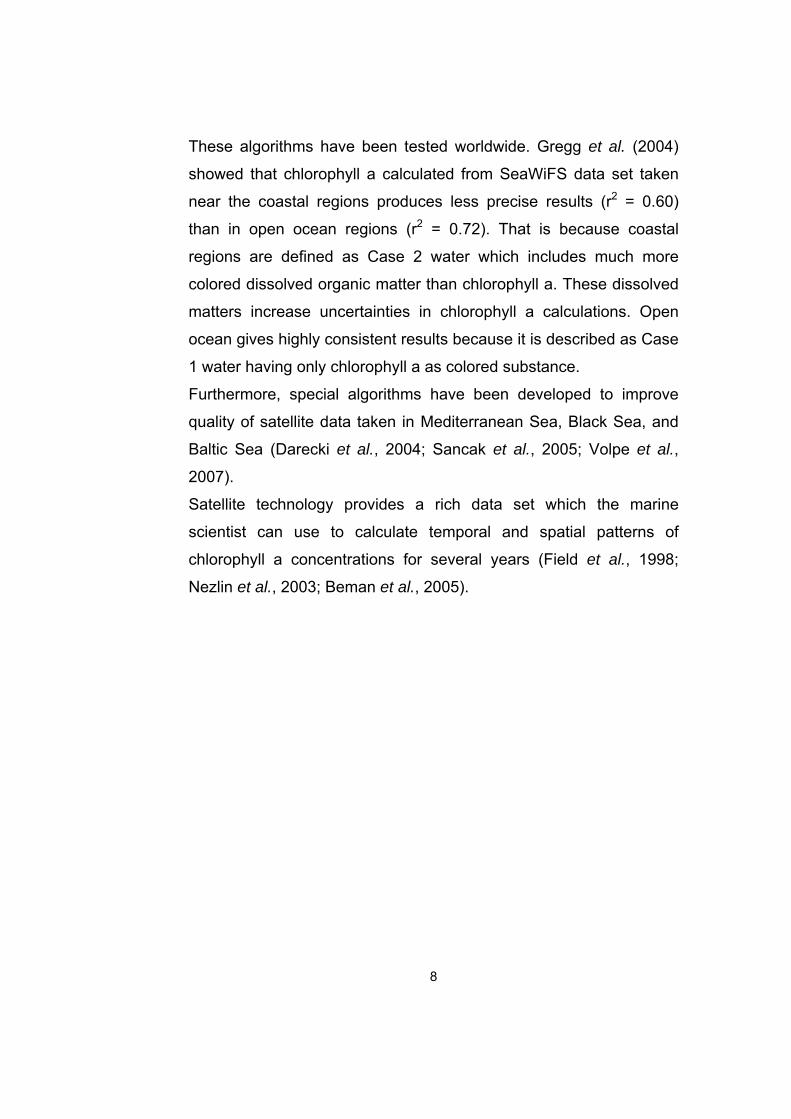
Of particular interest to our study is the 400-700 nm section of the

electromagnetic spectrum, called Photosynthetically Active Radiation

(PAR). PAR is used to calculate the chlorophyll a content of the

sampling area (Figure 2.1 and 2.2).

Figure 2.1 Electromagnetic Spectrum (URL 8).

16

Figure 2.2 Absorption Spectra of Chlorophyll a and b (URL 9).

2.1 SAMPLING SeaWiFS and MODIS-Aqua are two of the sensors which can be

used to calculate the amount of chlorophyll content of the sea

surface. This data can freely be acquired from The Ocean Biology

Processing Group (OBPG) which administers the data recorded by

both sensors. The spatial resolution of SeaWiFS data is 9x9

kilometers and that of MODIS-Aqua is 4X4 kilometers. In our study,

we have utilized data recorded by both sensors to evaluate

chlorophyll dynamics and the effect of climatic change.

SeaWiFS is a scanning radiometer collecting data since August 1997

through 8 spectral bands, whereas MODIS-Aqua is a scanning

radiometer collecting data since June 2002 with 36 spectral bands.

17

18

The major characteristics of MODIS and SeaWiFS spectral bands

are given in Table 2.1.

Table 2.1 MODIS-Aqua and SeaWiFS spectral bands used in ocean

color processing (Franz et al., 2005).

MODIS Band SeaWiFS Band MODIS

Wavelength

SeaWiFS

Wavelength

8 1 412 412

9 2 443 443

10 3 488 490

11 4 531 510

12 5 551 555

13 6 667 670

15 7 748 765

16 8 869 865

Radiances in bands 15 and 16 are used to evaluate atmospheric

contribution of observed radiance. The red band (670 nm) is used to

make corrections for NIR radiance leaving the ocean. These

calculations are necessary to remove the atmospheric noise from

chlorophyll radiance so that water-leaving radiance (Lw) can be

obtained. Thus the effects of solar illumination, viewing geometry and

atmospheric attenuation losses are corrected by using normalized Lw

(Franz et al., 2005).

The consistency and accuracy of MODIS and SeaWiFS data

acquired by Ocean Biology Discipline Processing Group (OBPG) is

very high. As indicated by Franz (2005), assessment of quality of the

data is maintained by comparison with in-situ observations, sensor-

to-sensor temporal comparisons, latitudinal trend comparisons,

cross-scan and detector dependent residuals.

It must be added that a large number of in-situ measurements

contributed by 43 institutions to SeaBASS which provides the

necessary in-situ information for the statistical validation of satellite

products (Figure 2.3). This cooperation has enabled researchers to

construct better algorithms so that the chlorophyll a content can be

calculated with utmost accuracy (Werdell and Bailey, 2002).

Figure 2.3 A map of all data points in the SeaBASS bio-optical data

set (Werdell and Bailey, 2002).

19

For the chlorophyll estimation, over 220,000 phytoplankton pigment

concentrations are collected by these institutions (Figure 2.4).

Figure 2.4 Maps of the distributions of chlorophyll a concentrations

(CHL) (Werdell and Bailey, 2002).

According to validation results of SeaWiFS and MODIS-Aqua

acquired by using in-situ match-ups (Figure 2.5 and 2.6), r2 for the

regressions are about 0.8 for each sensor (Bailey et al., 2006; URL

10).

20

Figure 2.5 In situ and SeaWiFS data set comparison

(Bailey et al., 2006).

Figure 2.6 In situ and MODIS-Aqua data set comparison (URL 10).

21

Marine Optical Buoy (MOBY) is another important data source for

calibrating these two sensors (Herring, 1994). The purpose of

MOBY’s mission is to detect penetrating and reflecting visible and

near-infrared radiation from the ocean. These measurements are

helpful to obtain time series databases for bio-optical algorithms such

as chlorophyll amount.

As a result of these various techniques and data analysis a visual

representation of chlorophyll a content for a particular location can be

obtained from OBPG. An example of such a map, which is also the

area of our study, is shown in Figure 2.7.

Figure 2.7 Chlorophyll a concentrations for the month of April, 2003

calculated from images taken by MODIS-Aqua.

22

23

2.2 DATA ANALYSIS Records of in situ measurements of sea surface temperature (SST)

data at the Turkish Meteorological Office are limited and some of it is

not of sufficient length for analyzing climatic fluctuations with the

exception of Tekirdağ Weather Station which we have used in this

study.

The remote sensing data which used in this study were recorded by

SeaWiFS and MODIS-Aqua sensors and have been downloaded

from the website of Ocean Biology Discipline Processing Group

(OBPG) (http://oceancolor.gsfc.nasa.gov/) (The acquisition of this

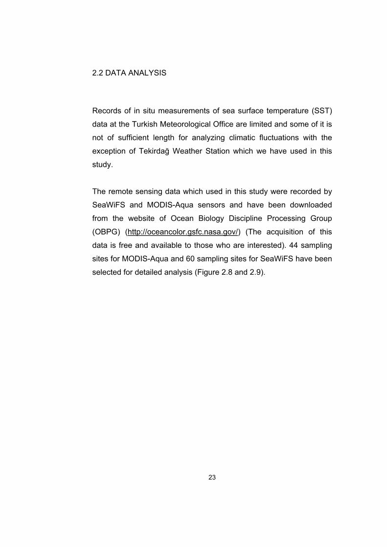
data is free and available to those who are interested). 44 sampling

sites for MODIS-Aqua and 60 sampling sites for SeaWiFS have been

selected for detailed analysis (Figure 2.8 and 2.9).

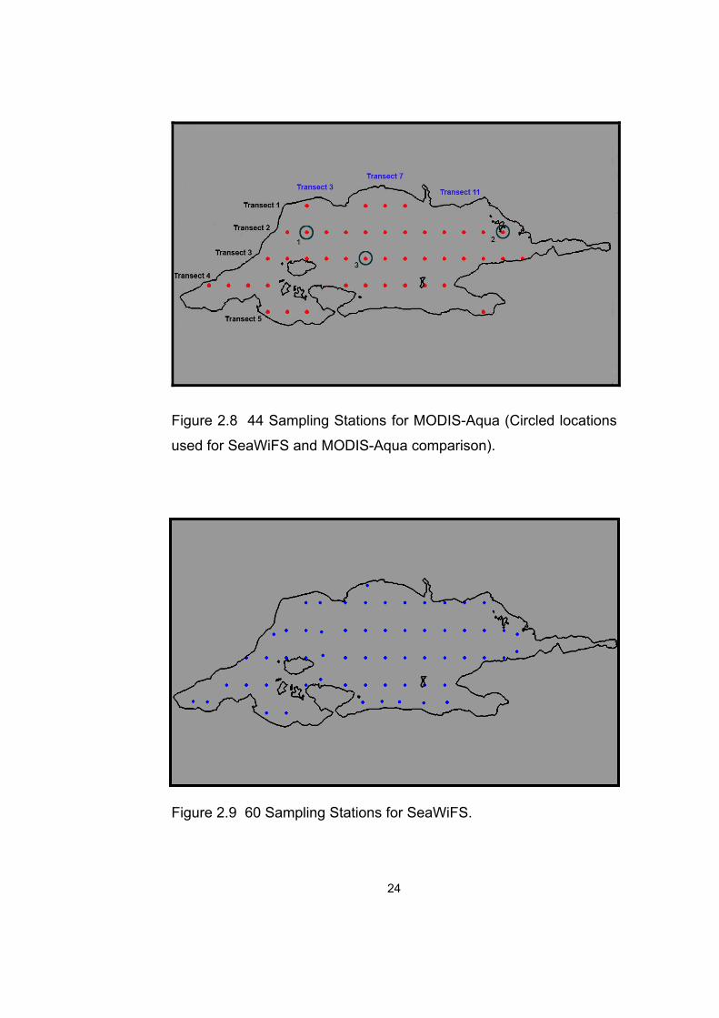
Figure 2.8 44 Sampling Stations for MODIS-Aqua (Circled locations

used for SeaWiFS and MODIS-Aqua comparison).

Figure 2.9 60 Sampling Stations for SeaWiFS.

24

25

For data processing and analysis we have used TNT mips 6.9, an

integrated Geographical Information System (GIS) and Remote

Sensing software ideally suited to handle large amounts of data.

As recommended by OBPG we have used the following equations to

calculate chlorophyll concentrations and SST:

Chlor_a= 10** ((0.015*pixel value) -2) for the MODIS-Aqua

chlorophyll data set,

SST= ((0.000717*pixel value)-2) for the MODIS-Aqua SST data set

and

Chlor_a= 10** ((0.000058*pixel value)-2) for SeaWiFS chlorophyll

data sets.

Where: Chlor_a: Chlorophyll Concentration in mg/m3

SST: Sea Surface Temperature in ºC.

Sancak et al. (2005) in a study lasting about a year involving the

Black Sea, Mediterranean and the Sea of Marmara reported that at

low concentrations some of the algorithms used for calculating

chlorophyll a content was not in complete agreement with in situ

measurements. Sancak et al. evaluated data taken by only

SeaWiFS. As we have stated earlier our analysis are based on data

taken both by SeaWiFS and MODIS-Aqua sensors. The remarkable

similarities between the data taken by both sensors, based on

monthly averages clearly indicate that our calculations are based on

data which are representative of the actual chlorophyll content

(Figure 3.1). Perhaps for analyses based on shorter time periods

improvements suggested by Sancak et al. (2005) are valid and

should be incorporated in such studies.

26

CHAPTER 3

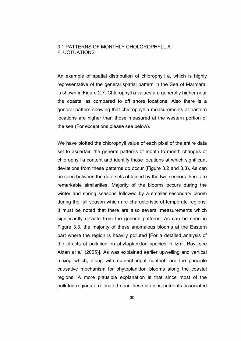
RESULTS AND DISCUSSION In order to assess the effects of climatic change a data set spanning

over several years is needed. Thus SeaWiFS set recorded during

1997- 2007 period is better suited for this type of analysis than

MODIS-Aqua data which covers a shorter period of 2002-2006.

However, it must be remembered that the spatial resolution of

MODIS-Aqua sensor is approximately 4 times better than those

recorded by SeaWiFS sensor. However a correlation analysis

between the two data sets obtained at three stations (Figure 2.8)

during 2002-2006 period is significantly correlated indicating that at

least when monthly averages are concerned either data set can be

used in place of the other. We consider this result as one of the most

importing finding in our study because of its possible applications in

other studies related to climate change. For studies requiring finer

resolution, which are too numerous to list here, MODIS-Aqua sensor

data should naturally be preferred.

In a sense these high correlations also verify the validity of several

algorithms developed by OBPG since both data sets has been

recorded by two independent sensors (Figure 3.1).

a) 1.Station:

0,002,004,006,008,00

10,0012,0014,0016,0018,0020,00

Sep-97

Mar-98

Sep-98

Mar-99

Sep-99

Mar-00

Sep-00

Mar-01

Sep-01

Mar-02

Sep-02

Mar-03

Sep-03

Mar-04

Sep-04

Mar-05

Sep-05

Mar-06

Sep-06

Mar-07

Time

Chl

orop

hyll

a C

once

ntra

tion

(mg/

m3 )

S1M1M2M3M4

0,002,004,006,008,00

10,0012,0014,0016,0018,00

Sep-

97

Mar

-98

Sep-

98

Mar

-99

Sep-

99

Mar

-00

Sep-

00

Mar

-01

Sep-

01

Mar

-02

Sep-

02

Mar

-03

Sep-

03

Mar

-04

Sep-

04

Mar

-05

Sep-

05

Mar

-06

Sep-

06

Mar

-07

Time

Chl

orop

hyll

a C

once

ntra

tion

(mg/

m3 ) S

M

27

b) 2.Station:

0,00

10,00

20,00

30,00

40,00

50,00

60,00

Sep-97

Mar-98

Sep-98

Mar-99

Sep-99

Mar-00

Sep-00

Mar-01

Sep-01

Mar-02

Sep-02

Mar-03

Sep-03

Mar-04

Sep-04

Mar-05

Sep-05

Mar-06

Sep-06

Mar-07

Time

Chl

orop

hyll

a C

once

ntra

tion

(mg/

m3 )

S1M1M2M3M4

0,00

5,00

10,00

15,00

20,00

25,00

30,00

35,00

Sep-97 Sep-98 Sep-99 Sep-00 Sep-01 Sep-02 Sep-03 Sep-04 Sep-05 Sep-06

Time

Chl

orop

hyll

a C

once

ntra

tion

(mg/

m3 )

SM

28

c) 3.Station:

0,00

5,00

10,00

15,00

20,00

25,00

Sep-97

Mar-98

Sep-98

Mar-99

Sep-99

Mar-00

Sep-00

Mar-01

Sep-01

Mar-02

Sep-02

Mar-03

Sep-03

Mar-04

Sep-04

Mar-05

Sep-05

Mar-06

Sep-06

Mar-07

Time

Chl

orop

hyll

a C

once

ntra

tion

(mg/

m3 )

S1M1M2M3M4

0,00

5,00

10,00

15,00

20,00

25,00

Sep-97 Sep-98 Sep-99 Sep-00 Sep-01 Sep-02 Sep-03 Sep-04 Sep-05 Sep-06

Time

Chl

orop

hyll

a C

once

ntra

tion

(mg/

m3 )

SM

Figure 3.1 Chlorophyll a contents of 3 stations calculated by using

SeaWiFS and MODIS-Aqua data sets. Correlation coefficients (r)

between SeaWiFS and MODIS-Aqua for each stations are 0.87 (a),

0.83 (b) and 0.91 (c). The results are statistically significant at 1%

level.

(S and S1: Chlorophyll a contents of SeaWiFS sampling station; M1,

M2, M3 and M4: Average Chlorophyll a contents of MODIS-Aqua

sampling stations)

29

30

3.1 PATTERNS OF MONTHLY CHOLOROPHYLL A FLUCTUATIONS An example of spatial distribution of chlorophyll a, which is highly

representative of the general spatial pattern in the Sea of Marmara,

is shown in Figure 2.7. Chlorophyll a values are generally higher near

the coastal as compared to off shore locations. Also there is a

general pattern showing that chlorophyll a measurements at eastern

locations are higher than those measured at the western portion of

the sea (For exceptions please see below).

We have plotted the chlorophyll value of each pixel of the entire data

set to ascertain the general patterns of month to month changes of

chlorophyll a content and identify those locations at which significant

deviations from these patterns do occur (Figure 3.2 and 3.3). As can

be seen between the data sets obtained by the two sensors there are

remarkable similarities. Majority of the blooms occurs during the

winter and spring seasons followed by a smaller secondary bloom

during the fall season which are characteristic of temperate regions.

It must be noted that there are also several measurements which

significantly deviate from the general patterns. As can be seen in

Figure 3.3, the majority of these anomalous blooms at the Eastern

part where the region is heavily polluted [For a detailed analysis of

the effects of pollution on phytoplankton species in Izmit Bay, see

Aktan et al. (2005)]. As was explained earlier upwelling and vertical

mixing which, along with nutrient input content, are the principle

causative mechanism for phytoplankton blooms along the coastal

regions. A more plausible explanation is that since most of the

polluted regions are located near these stations nutrients associated

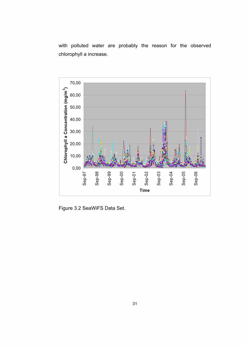
with polluted water are probably the reason for the observed

chlorophyll a increase.

0,00

10,00

20,00

30,00

40,00

50,00

60,00

70,00S

ep-9

7

Sep

-98

Sep

-99

Sep

-00

Sep

-01

Sep

-02

Sep

-03

Sep

-04

Sep

-05

Sep

-06

Time

Chl

orop

hyll

a C

once

ntra

tion

(mg/

m3 )

Figure 3.2 SeaWiFS Data Set.

31

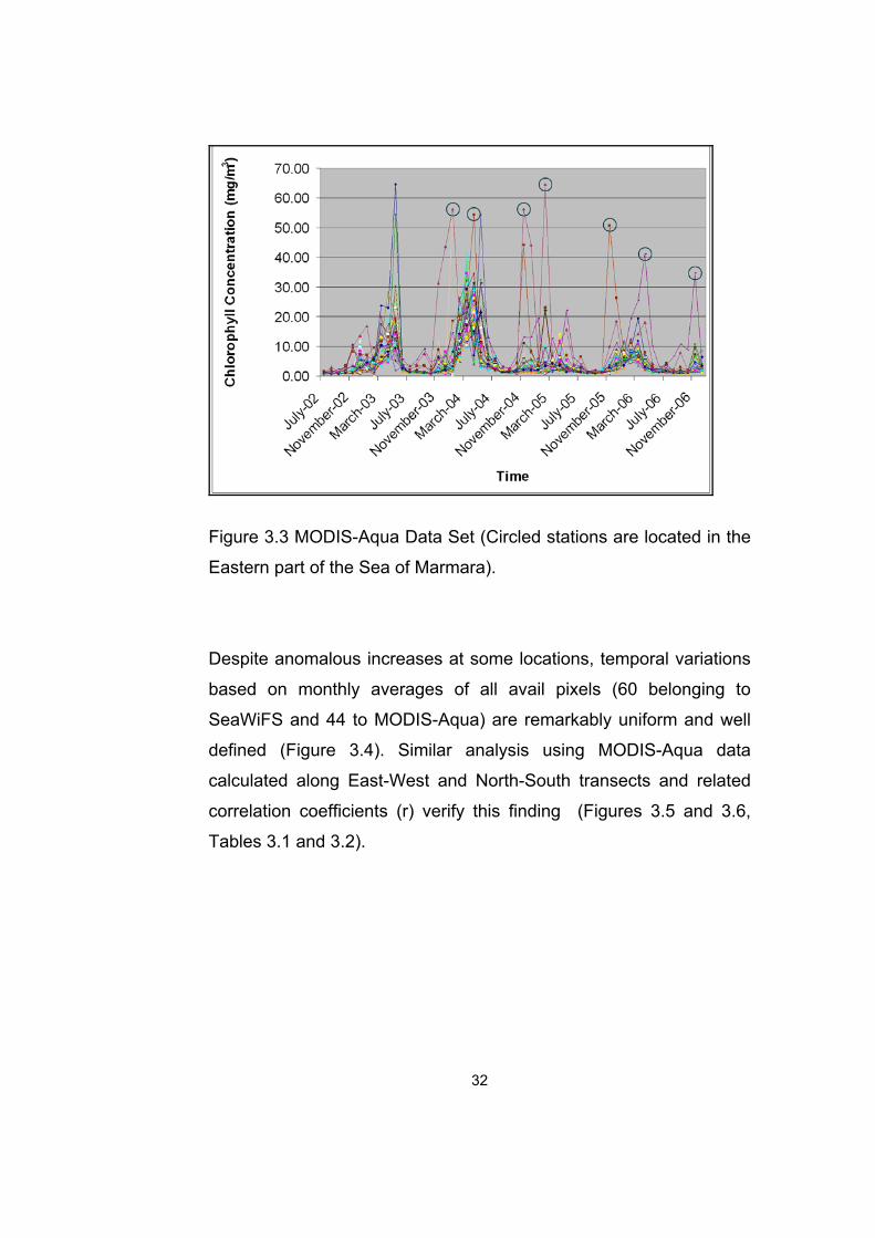
Figure 3.3 MODIS-Aqua Data Set (Circled stations are located in the

Eastern part of the Sea of Marmara).

Despite anomalous increases at some locations, temporal variations

based on monthly averages of all avail pixels (60 belonging to

SeaWiFS and 44 to MODIS-Aqua) are remarkably uniform and well

defined (Figure 3.4). Similar analysis using MODIS-Aqua data

calculated along East-West and North-South transects and related

correlation coefficients (r) verify this finding (Figures 3.5 and 3.6,

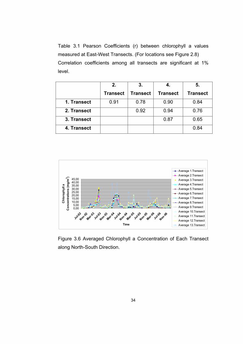
Tables 3.1 and 3.2).

32

0,00

5,00

10,00

15,00

20,00

25,00

Sep-97

Mar-98

Sep-98

Mar-99

Sep-99

Mar-00

Sep-00

Mar-01

Sep-01

Mar-02

Sep-02

Mar-03

Sep-03

Mar-04

Sep-04

Mar-05

Sep-05

Mar-06

Sep-06

Mar-07

Time

Chl

orop

hyll

a C

once

ntra

tion

(mg/

m3 )

SeaWiFSMODIS-Aqua

Figure 3.4 Time Series of Monthly Averages of Chlorophyll a

Concentrations during 1997-2007 based on SeaWiFS and MODIS-

Aqua data sets.

0,005,00

10,0015,0020,0025,0030,0035,0040,0045,00

Jul-0

2

Nov-02

Mar-03

Jul-03

Nov-03

Mar-04

Jul-04

Nov-04

Mar-05

Jul-0

5

Nov-05

Mar-06

Jul-06

Nov-06

Time

Chl

orop

hyll

a C

once

ntra

tion

(mg/

m3 )

Average 1.TransectAverage 2.TransectAverage 3.TransectAverage 4.TransectAverage 5.Transect

Figure 3.5 Averaged Chlorophyll a Concentration of Each Transect

along East-West Direction.

33

34

Table 3.1 Pearson Coefficients (r) between chlorophyll a values

measured at East-West Transects. (For locations see Figure 2.8)

Correlation coefficients among all transects are significant at 1%

level.

2.

Transect 3.

Transect4.

Transect 5.

Transect

1. Transect 0.91 0.78 0.90 0.84

2. Transect 0.92 0.94 0.76

3. Transect 0.87 0.65

4. Transect 0.84

0,005,00

10,0015,0020,0025,0030,0035,0040,0045,00

Jul-0

2

Nov-02

Mar-03

Jul-0

3

Nov-03

Mar-04

Jul-0

4

Nov-04

Mar-05

Jul-0

5

Nov-05

Mar-06

Jul

Time

Chl

orop

hyll

a C

once

ntra

tions

(mg/

m3 )

-06

Nov-06

Average 1.TransectAverage 2.TransectAverage 3.TransectAverage 4.TransectAverage 5.TransectAverage 6.TransectAverage 7.TransectAverage 8.TransectAverage 9.TransectAverage 10.TransectAverage 11.TransectAverage 12.TransectAverage 13.Transect

Figure 3.6 Averaged Chlorophyll a Concentration of Each Transect

along North-South Direction.

1. Tran. 2. Tran. 3. Tran. 4. Tran. 5. Tran. 6. Tran. 7. Tran. 8. Tran. 9. Tran. 10. Tran. 11. Tran. 12. Tran. 2. Tran. 0.97 3. Tran. 0.96 0.964. Tran. 0.83 0.85 0.855. Tran. 0.81 0.90 0.82 0.896. Tran. 0.83 0.90 0.84 0.95 0.967. Tran. 0.84 0.88 0.84 0.98 0.93 0.998. Tran. 0.82 0.87 0.82 0.96 0.94 0.98 0.98 9. Tran. 0.75 0.82 0.77 0.93 0.92 0.94 0.94 0.94 10. Tran. 0.81 0.85 0.82 0.92 0.88 0.91 0.91 0.91 0.97 11. Tran. 0.67 0.70 0.67 0.72 0.73 0.74 0.74 0.75 0.82 0.8912. Tran. 0.68 0.71 0.67 0.71 0.71 0.71 0.71 0.69 0.70 0.69 0.5813. Tran. 0.57 0.54 0.53 0.64 0.57 0.61 0.63 0.66 0.63 0.67 0.61 0.61

Table 3.2 Pearson Coefficients (r) between chlorophyll a values measured at North- South Transects.

(For locations see Figure 2.8) Correlation coefficients among all transects are significant at 1% level.

(Tran: Transect)

35

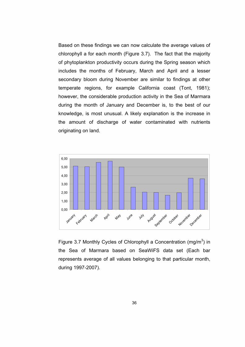
Based on these findings we can now calculate the average values of

chlorophyll a for each month (Figure 3.7). The fact that the majority

of phytoplankton productivity occurs during the Spring season which

includes the months of February, March and April and a lesser

secondary bloom during November are similar to findings at other

temperate regions, for example California coast (Tont, 1981);

however, the considerable production activity in the Sea of Marmara

during the month of January and December is, to the best of our

knowledge, is most unusual. A likely explanation is the increase in

the amount of discharge of water contaminated with nutrients

originating on land.

0,00

1,00

2,00

3,00

4,00

5,00

6,00

Janu

ary

Februa

ryMarc

hApri

lMay

June Ju

ly

Augus

t

Septem

ber

Octobe

r

November

December

Figure 3.7 Monthly Cycles of Chlorophyll a Concentration (mg/m3) in

the Sea of Marmara based on SeaWiFS data set (Each bar

represents average of all values belonging to that particular month,

during 1997-2007).

36

37

3.2 SST and CHLOROPHYLL a CORRELATIONS In a recent paper by Gregg et al. (2003) it was reported that globally,

since 1980’es there has been 6% decrease in annual marine primary

production and they attribute this decrease to global warming. As can

be easily seen in several graphs presented above we have not seen

a similar decrease in primary productivity in the Sea of Marmara. Sea

surface temperatures (SST) measured near Tekirdağ by Turkish

Meteorological Office (1997-2007) and those recorded by MODIS-

Aqua (2002-2006) do not show any significant increase in SST

values (Figure 3.8). Since our study area is highly localized

compared to Gregg et al.’s (2003) there might have been mitigating

circumstances, such as local discharges, offsetting the effects of

global warming.

However, as has been discussed in Chapter 1, even though

temperature change itself may not effect primary production directly it

may be indicative of other processes such as upwelling and vertical

mixing. Lowering of SST in the sea has been recognized as a

signature of upwelling and vertical mixing since during this process

the warm surface waters are replaced by the colder subsurface

waters. Indeed, correlations between monthly averages of SST and

corresponding chlorophyll a values are statistically significant

(inverse) at 1% level where r= -0.53 and the equation of the fitted

model is:

Chlorophyll a = 7.09199 – 0.215402* SST

(For details see Appendix A)

0

5

10

15

20

25

30

Sep-97

Mar-98

Sep-98

Mar-99

Sep-99

Mar-00

Sep-00

Mar-01

Sep-01

Mar-02

Sep-02

Mar-03

Sep-03

Mar-04

Sep-04

Mar-05

Sep-05

Mar-06

Sep-06

Mar-07

Time

oC TekirdagMODIS-Aqua

Figure 3.8 Sea Surface Temperature (SST) during 1997-2007.

38

39

CHAPTER 4

CONCLUSIONS AND RECOMMENDATIONS FOR FUTURE STUDIES

Our findings presented in this thesis in addition to their intrinsic

scientific value will also have practical applications in both marine

biology and remote sensing studies. The wealth of data we were

fortunate to acquire enabled us to try a variety of techniques and

calculations resulting in such applications. For example we have

found that MODIS-Aqua and SeaWiFS chlorophyll data can be used

interchangeably if the analysis is based on monthly averages.

Similarly a few well chosen transects consisting of a handful of

stations can be used as representative of the entire region. More

importantly although Roden (1960) have shown that along

southwestern region of the Pacific Ocean, monthly averages of SST

show coherence for nearly 200 kilometers, still it was surprising for

us to find out that in a much more complex location such as Marmara

Sea, SST measurements taken at a single station (Tekirdağ) will be

representative of the entire area and these values will be almost

identical to those recorded by satellite sensors.

The fact that either SST or Chlorophyll a value can be approximated

when one is unknown by using a fitted linear model which is

statistically sound will again be of great use not only for basic

research but for practical applications such as assessing the effects

of pollutants at major discharge locations.

40

We believe a cross comparison of chlorophyll a values calculated by

remote sensing techniques at several locations in Mediterranean,

Aegean and Black Sea will be most interesting. Also, monitoring the

major affluent discharge stations by using data taken at shorter time

intervals and with more resolution can be very beneficial for

evaluating the effects of pollution on primary production.

41

REFERENCES Aktan, Y., Tüfekçi, V., Tüfekçi, H., Aykulu, G. (2005) Distribution Patterns, Biomass Estimates and Diversity of Phytoplankton in Izmit Bay (Turkey). Estuarine, Coastal and Shelf Science. Vol.64, pp. 372-384. Bailey, S. W. and Werdell, P. J. (2006) A Multi-Sensor Approach for the On-Orbit Validation of Ocean Color Satellite Data Products. Remote Sensing of Environment, Vol. 102, 19 January, pp.12-23. Behrenfeld, M. J., Bale, A. J., Kolber, Z. S., Aiken, J., Falkowski, P. G. (1996) Confirmation of Iron Limitation of Phytoplankton Photosynthesis in the Equatorial Pacific Ocean. Nature, Vol. 383, 10 October, pp. 508-511. Beman, J.M., Arrigo, K.R., Matson, P.A. (2005) Agricultural Runoff Fuels Large Phytoplankton Blooms in Vulnerable Areas of the Ocean. Nature, Vol. 434, 10 March, pp. 211-214. Besiktepe, S. (1991) Some Aspects of the Circulation and Dynamics of the Sea of Marmara. PhD. Thesis, Institute of Marine Sciences, Middle East Technical University, Erdemli, Içel, 226 pp. Besiktepe, S., Sur, H. İ., Ozsoy, E., Latif, M. A., Oguz, T., Unluata, U. (1994) Circulation and hydrography of the Sea of Marmara. Progress in Oceanography, Vol. 34, pp. 285-334. Bigg, G.R., Jickells, T.D., Liss, P.S., Osborn, T.J. (2003) Review: The Role of the Ocean in Climate. International Journal of Climatology. Vol. 23. pp. 1127–1159.

42

Blain, S., Quéguiner, B., Armand, L., Belviso, S., Bombled, B., Bopp, L., Bowie, A., Brunet, C., Brussaard, C., Carlotti, F., Christaki, U., Corbière, A., Durand, I., Ebersbach, F., Fuda, J., Garcia, N., Gerringa, L., Griffiths, B., Guigue, C., Guillerm, C., Jacquet, S., Jeandel, C., Laan, P., Lefèvre, D., Monaco, C., Malits, A., Mosseri, J., Obernosterer, I., Park, Y., Picheral, M., Pondaven, P., Remenyi, T., Sandroni, V., Sarthou, G., Savoye, N., Scouarnec, L., Souhaut, M., Thuiller, D., Timmermans, K., Trull, T., Uitz, J., Beek, P., Veldhuis, M., Vincent, D., Viollier, E., Vong L., Wagener, T. (2007) Effect of Natural Iron Fertilization on Carbon Sequestration in the Southern Ocean. Nature, Vol.446, 26 April, pp.1070-1074. Boyd, P. W., Watson, A. J., Law, C. S., Abraham, E. R., Trull, T., Murdoch, R., Bakker, D. C. E., Bowie, A. R., Buesseler, K. O., Chang, H., Charette, M., Croot, P., Downing, K., Frew, R., Gall, M., Hadfield, M., Hall, J., Harvey, M., Jameson, G., LaRoche, J., Liddicoat, M., Ling, R., Maldonado, M. T., McKay, R. M., Nodder, S., Pickmere, S., Pridmore, R., Rintoul, S., Safl, K., Sutton, P., Strzepek, R., Tanneberger, K., Turner, S., Waite, A., Zeldis, J. (2000) A Mesoscale Phytoplankton Bloom in the Polar Southern Ocean Stimulated by Iron Fertilization. Nature, Vol. 407, 12 October, pp. 695-702. Cloern, J.E. (1996) Phytoplankton Bloom Dynamics in Coastal Ecosystems: A Review with Some General Lessons from Sustained Investigation of San Francisco Bay, California. Reviews of Geophysics, Vol.34, No.2, May. pp. 127-168. Darecki, M. and Stramski, D. (2004) An Evaluation of MODIS and SeaWiFS Bio-Optical Algorithms in the Baltic Sea. Remote Sensing of Environment, Vol.89, pp. 326-350. Esaias, W.E., Abbott, M.R., Barton, I., Brown, O.B., Campbell, J.W., Carder, K.L., Clark, D.K., Evans, R.H., Hoge, F.E., Gordon, H.R., Balch, W.M., Letelier, R., Minnett, P.J. (1998) An Overview of MODIS Capabilities for Ocean Science Observations. IEEE Transactions on Geoscience and Remote Sensing, Vol.36, No.4, July, pp. 1250-1265.

43

Everett, J. and Simonett, D.S. (1976) Remote Sensing of Environment. Edited by Joseph L, Jr. and David S. Simonett. Addison-Wesley Publishing Company, USA. p.105. Field, C.B., Behrenfeld, M.J., Randerson, J.T., Falkowski, P. (1998) Primary Production of the Biosphere: Integrating Terrestrial and Oceanic Components. Science, Vol. 281, pp. 237-240. Franz, B.A., Bailey, S.W., Eplee Jr., R.E., Feldman, G.C., Kwiatkowska, E., McClain, C., Meister, G., Patt, F.S., Thomas, D., Werdell, P.J. (2005) The Continuity of Ocean Color Measurements from SeaWiFS to MODIS. In J.J. Butler (Ed.), Earth Observing Systems: X.Proceedings SPIE, The International Society for Optical Engineering. Vol. 5882, pp.49-60. Franz, B. (2005) Methods for Assessing the Quality and Consistency of Ocean Color Products, Ocean Biology Processing Group, 18 January 2005, http://oceancolor.gsfc.nasa.gov/DOCS/methods/ Garrison, T. (2005) Oceanography, 5th edition. Thomson Brooks/Cole, USA. pp. 217, 342-345. Gregg, W.W., Conkright, M.E., Ginoux, P., O, Reilly, J.E., Casey, N.W. (2003) Ocean Primary Production and Climate: Global Decadal Changes. Geophysical Research Letters. Vol. 30, No. 15, 1809, doi:10.1029 /2003GL016889, pp. OCE 3.1-3.4. Gregg, W.W. and Casey, N.W. (2004) Global and Regional Evaluation of the SeaWiFS Chlorophyll Data Set. Remote Sensing of Environment, Vol.93, pp. 463-479. Herring, D. (1994) MODIS/SeaWiFS Team Deploys Marine Optical Buoy, Continues Marine Optical Characterization Experiment. The Earth Observer, January/February.

44

Hovis, W.A, Clark, D.K., Anderson, F., Austin, R.W., Wilson, W.H., Baker, E.T., Ball, D., Gordon, H.R., Mueller, J.L., El-Sayed, S.Z., Sturm, B., Wrigley, R.C., Yentsch, C.S. (1980) Nimbus-7 Coastal Zone Color Scanner: System Description and Initial Imagery. Science, NewSeries, Vol. 210, No.4465, October 3, pp. 60-63. Nezlin, N.P. and Li, B.L. (2003) Time-Series Analysis of Remote-Sensed Chlorophyll and Environmental Factors in the Santa Monica-San Pedro Basin off Southern California. Journal of Marine Systems, Vol.39, pp. 185-202. O’Reilly, J.E., Maritorena, S., Mitchell, B.G., Siegel, D.A., Carder, K.L., Garver, S.A., Kahru, M., McClain,C. (1998) Ocean Color Chlorophyll Algorithms for SeaWiFS. Journal of Geophysical Research, Vol.103, No.C11, October 15, pp.24,937-24,953. O’Reilley, J.E., Maritorena, S., O’Brien, M.C., Siegel, D.A., Toole, D., Menzies, D., Smith, R.C., Mueller, J.L., Mitchell, B.G., Kahru, M., Cota, G.F., Hooker, S.B., McClain, C.R., Carder, K.L., Karger, F.M., Harding, L., Magnuson, A., Phinney, D., Moore, G.F., Aiken, J., Arrigo, K.R., Letelier, R., Culver, M. (2000) SeaWiFS Postlaunch Calibration and Validation Analyses, Part 3. NASA Technical Memorandum, Vol.11, No. 2000-206892, pp. 1-48. Polat, S. C. and Tugrul, S. (1995) Nutrient and Organic Carbon Exchanges between the Black and Marmara Seas through the Bosporus Strait. Continental Shelf Research, Vol. 15, No.9, pp. 1115-1132. Purves, W.K., Sadava, D., Orians, G.H., Heller, H.C. (2001) Life, the Science of Biology, 6th edition. Sinauer Associates, Inc. W.H. Freeman and Company, USA. pp. 480-494. Richardson, L. L. (1996) Remote Sensing of Algal Bloom Dynamics. BioScience, Vol.46, No.7 (Jul.-Aug.), pp.492-501.

45

Roden, G. I. (1960) On Nonseasonal Temperature and Salinity Variations along the West Coast of the United States and Canada. CalCOFI Prog. Rpts. Vol.8, pp. 95-119. Rosen, T., and Duffy, J. E. (2007) Open Ocean Iron Fertilization. In: Encyclopedia of Earth. Eds. Cutler J. Cleveland [Published May 22, 2007; Retrieved October 22, 2007]. http://www.eoearth.org/article/Open_ocean_iron_fertilization Sabins, F.F. (1997) Remote Sensing: Principles and Interpretation, 3rd edition. W.H. Freeman and Company, New York. p.1. Sancak, S., Besiktepe, S. T., Yilmaz, A., Lee, M., Frouin, R. (2005) Evaluation of SeaWiFS Chlorophyll-a in the Black and Mediterranean Seas. International Journal of Remote Sensing, Vol. 26, No. 10, 20 May, pp. 2045–2060. Stowe, K. (1996) Exploring Ocean Science, 2nd edition. John Wiley & Sons, Inc., USA. pp. 276-277. Stumpf, R. P. (2001) Applications of Satellite Ocean Color Sensors for Monitoring and Predicting Harmful Algal Blooms. Human and Ecological Risk Assessment, Vol.7, No.5, pp.1363 – 1368. Tont, S. (1981) Temporal Variations in Diatom Abundance off Southern California in Relation to Surface Temperature, Air Temperature and Sea Level. Journal of Marine Research, Vol. 39, No.1, pp. 191-201. Tugrul, S. and Polat, C. (1995) Quantitative Comparison of the Influxes of Nutrients and Organic Carbon into the Sea of Marmara both from Anthropogenic Sources and from the Black Sea. Wat. Sci. Tech. Vol. 32, No. 2, pp. 115-121. Turkish Meteorological Office Data Reports, Ankara.

46

Unluata, U., Oguz, T., Latif, M. A., Ozsoy, E. (1990) On the Physical Oceanography of the Turkish Straits. In: The Physical Oceanography of Sea Straits, L.J. Pratt, (Ed.), NATO/ASI series, Kluwer, pp. 25-60. URL 1: NASA, Visible Earth, Sea of Marmara, Turkey, http://visibleearth.nasa.gov/view_rec.php?id=5652 Last update on June 08, 2006, last accessed in August 2007. URL 2: NASA’s Observatorium, http://observe.arc.nasa.gov/nasa/exhibits/history/history_index.html Last update on 1998, last accessed in August 2007. URL 3: NASA, Sputnik and The Dawn of the Space Age, http://history.nasa.gov/sputnik/ Last update on January 19, 2007, last accessed in August 2007. URL 4: Current Ocean-Color Sensors http://www.ioccg.org/sensors/current.html Last update on April 30, 2007, last accesses in August 2007. URL 5: Ocean Color Documents http://oceancolor.gsfc.nasa.gov/DOCS/MSL12/master_prodlist.html/#chlor_a Last accessed in August 2007. URL 6: Natural History Museum, http://piclib.nhm.ac.uk/piclib/www/ Last update on 2005, last accessed in August 2007. URL 7: What are Eddies?, http://www.geol.sc.edu/cbnelson/eddy/eddy.htm Last accessed in August 2007. URL 8: Coastal Carolina University, Physical Oceanography Animations, http://kingfish.coastal.edu/marine/Animations/ Last accessed in August 2007.

47

URL 9: Chlorophyll, Paul May, School of Chemistry, University of Bristol, http://www.chm.bris.ac.uk/motm/chlorophyll/chlorophyll_h.htm Last accessed in August 2007. URL 10: MODIS-Aqua Validation Results, http://seabass.gsfc.nasa.gov/cgi-bin/matchup_results.cgi?sensor=a, Last update on 06 August 2007, last accessed in August 2007. Volpe, G., Santoleri, R., Vellucci, V., Alcalà, M.R., Marullo, S., Ortenzio, F.D. (2007) The Color of the Mediterranean Sea: Global versus Regional Bio-Optical Algorithms Evaluation and Implication for Satellite Chlorophyll Estimates. Remote Sensing of Environment, Vol. 107, pp. 625-638. Werdell, P. J. and Bailey, S. W. (2002) The SeaWiFS Bio-Optical Archive and Storage System (SeaBASS): Current Architecture and Implementation. NASA/TM-2002-211617. pp. 1-45.

48

APPENDIX A

Regression analysis between monthly averages of sea surface

temperature (SST) and Chlorophyll a concentration is shown during

1997-2007 period. Chlorophyll values have been recorded by

SeaWiFS. SST values are obtained from Tekirdağ Meteorological

Station.

Coefficients Least

Squares Standard T

Parameter Estimate Error Statistic P-Value

Intercept 7.09199 0.546969 12.966 0.0000 Slope -0.215402 0.0321747 -6.69477 0.0000 Analysis of Variance Source Sum of

Squares Df Mean

Square F-Ratio

P-Value

Model 207.375 1 207.375 44.82 0.0000 Residual 522.835 113 4.62686 Total (Corr.)

730.21 114

Correlation Coefficient = -0.532911

R-squared = 28.3994 percent

R-squared (adjusted for d.f.) = 27.7658 percent

Standard Error of Est. = 2.15101

Mean absolute error = 1.23675

Durbin-Watson statistic = 0.722076 (P=0.0000)

49

Lag 1 residual autocorrelation = 0.630902

The output shows the results of fitting a linear model to describe the

relationship between Chlorophyll a Concentration and SST. The

equation of the fitted model is

Chlorophyll a Concentration = 7.09199 - 0.215402* SST

Since the P-value in the ANOVA table is less than 0.05, there is a

statistically significant relationship between Chlorophyll a

Concentration and SST at the 95.0% confidence level.

The R-Squared statistic indicates that the model as fitted explains

28.3994% of the variability in Chlorophyll a Concentration. The

correlation coefficient equals -0.532911, indicating a moderately

strong relationship between the variables. The standard error of the

estimate shows the standard deviation of the residuals to be

2.15101.

Since the P-value is less than 0.05, there is an indication of possible

serial correlation at the 95.0% confidence level.