Temporal and Spatial Analysis of GNSS network data for

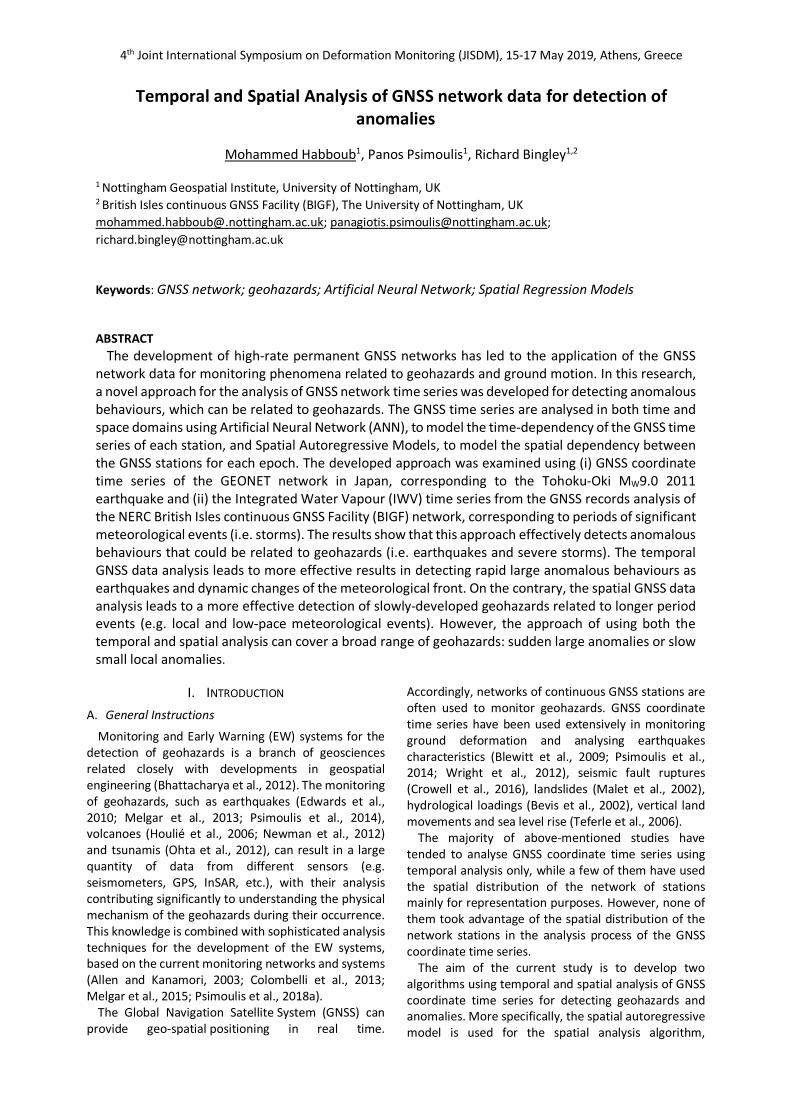
4th Joint International Symposium on Deformation Monitoring (JISDM), 15-17 May 2019, Athens, Greece

Temporal and Spatial Analysis of GNSS network data for detection of anomalies

Mohammed Habboub1, Panos Psimoulis1, Richard Bingley1,2

1 Nottingham Geospatial Institute, University of Nottingham, UK 2 British Isles continuous GNSS Facility (BIGF), The University of Nottingham, UK [email protected]; [email protected]; [email protected] Keywords: GNSS network; geohazards; Artificial Neural Network; Spatial Regression Models ABSTRACT

The development of high-rate permanent GNSS networks has led to the application of the GNSS network data for monitoring phenomena related to geohazards and ground motion. In this research, a novel approach for the analysis of GNSS network time series was developed for detecting anomalous behaviours, which can be related to geohazards. The GNSS time series are analysed in both time and space domains using Artificial Neural Network (ANN), to model the time-dependency of the GNSS time series of each station, and Spatial Autoregressive Models, to model the spatial dependency between the GNSS stations for each epoch. The developed approach was examined using (i) GNSS coordinate time series of the GEONET network in Japan, corresponding to the Tohoku-Oki MW9.0 2011 earthquake and (ii) the Integrated Water Vapour (IWV) time series from the GNSS records analysis of the NERC British Isles continuous GNSS Facility (BIGF) network, corresponding to periods of significant meteorological events (i.e. storms). The results show that this approach effectively detects anomalous behaviours that could be related to geohazards (i.e. earthquakes and severe storms). The temporal GNSS data analysis leads to more effective results in detecting rapid large anomalous behaviours as earthquakes and dynamic changes of the meteorological front. On the contrary, the spatial GNSS data analysis leads to a more effective detection of slowly-developed geohazards related to longer period events (e.g. local and low-pace meteorological events). However, the approach of using both the temporal and spatial analysis can cover a broad range of geohazards: sudden large anomalies or slow small local anomalies.

I. INTRODUCTION

A. General Instructions

Monitoring and Early Warning (EW) systems for the detection of geohazards is a branch of geosciences related closely with developments in geospatial engineering (Bhattacharya et al., 2012). The monitoring of geohazards, such as earthquakes (Edwards et al., 2010; Melgar et al., 2013; Psimoulis et al., 2014), volcanoes (Houlié et al., 2006; Newman et al., 2012) and tsunamis (Ohta et al., 2012), can result in a large quantity of data from different sensors (e.g. seismometers, GPS, InSAR, etc.), with their analysis contributing significantly to understanding the physical mechanism of the geohazards during their occurrence. This knowledge is combined with sophisticated analysis techniques for the development of the EW systems, based on the current monitoring networks and systems (Allen and Kanamori, 2003; Colombelli et al., 2013; Melgar et al., 2015; Psimoulis et al., 2018a).

The Global Navigation Satellite System (GNSS) can provide geo-spatial positioning in real time.

Accordingly, networks of continuous GNSS stations are often used to monitor geohazards. GNSS coordinate time series have been used extensively in monitoring ground deformation and analysing earthquakes characteristics (Blewitt et al., 2009; Psimoulis et al., 2014; Wright et al., 2012), seismic fault ruptures (Crowell et al., 2016), landslides (Malet et al., 2002), hydrological loadings (Bevis et al., 2002), vertical land movements and sea level rise (Teferle et al., 2006).

The majority of above-mentioned studies have tended to analyse GNSS coordinate time series using temporal analysis only, while a few of them have used the spatial distribution of the network of stations mainly for representation purposes. However, none of them took advantage of the spatial distribution of the network stations in the analysis process of the GNSS coordinate time series.

The aim of the current study is to develop two algorithms using temporal and spatial analysis of GNSS coordinate time series for detecting geohazards and anomalies. More specifically, the spatial autoregressive model is used for the spatial analysis algorithm,


assuming that the GNSS coordinate time series from a network of stations are spatially dependent. Whereas, for the temporal analysis algorithm, where the GNSS coordinate time series of a single station is temporally dependent, Artificial Neural Networks are used to extract the temporal dependency. By following this approach, the behaviour of GNSS coordinate time series will be monitored not only regarding the history of the time series of a station but regarding its spatial context as well, which creates a new perspective in monitoring using such time series.

To evaluate the performance of the two algorithms, they were used in the analysis of GNSS data in two different applications: (i) for the analysis of the 1Hz GNSS coordinate time series of the GEONET network in Japan, corresponding to the time interval of the Tohoku-Oki 2011 Mw9.0 earthquake and (ii) for the analysis of GNSS Integrated Water Vapour (IWV) time series derived by the British Isles continuous GNSS Facility (BIGF), and the detection of anomalies which could be related to strong rainfall events in the UK.

II. METHODOLOGY

In this study, two different types of GNSS time series are analysed. For the case study of Tohoku-Oki 2011 earthquake, the GNSS coordinate time series of North, East, Up (NEU) displacements were combined to form the 3D GNSS coordinate time series which were used as inputs for the two algorithms. For the case of GNSS IWV time series, these were derived directly from as part of the process of the BIGF GPS network data. The GNSS time series were split into two datasets: (i) the algorithm-training dataset, which is a part in the beginning of the time series used for the training of the algorithms; and (ii) the algorithm-testing dataset, which is the part of the time series following that of the algorithm-training dataset and is used to test the performance of the algorithms. The main aim of algorithm-training dataset is to model the characteristics of the GNSS time series. Initially, each GNSS time series were de-trended to remove any potential long-term linear trend (i.e. tectonic motion, etc.). Then, the GNSS time series were analysed using in-house developed Discrete Fourier Transform (DFT) to identify the characteristics of the time series in the frequency domain. Based on the spectrum of each GNSS time series, a cut-off frequency was defined and a Butterworth low-pass filter was designed to filter out all high frequencies of the time series, and finally obtain the low-frequency component of the detrended time series (i.e. the low-frequency time series) of each station in a network. The purpose of this stage was to train the Artificial Neural Network and to use the calculated statistics (i.e. means and standard deviations) as parameters in the next stage (i.e. the algorithm-testing stage).

A. The spatial analysis algorithm

In this algorithm, a special simplified version of the Manski (1993) model, the First-order AutoRegressive (FAR) model was used based on the assumption that the spatial dependency of the studied values is a function of internal interactions only. More specifically, the FAR model which was used is expressed by the following equation (LeSage, 1998):

𝑌 = 𝜌𝑾𝑌+ 𝜀 (1)

where Y = N x 1 vector representing the values of the

low frequency time series ρ = the spatial autoregressive parameter W=NxN matrix defining the spatial relationship between the N stations ε= the spatial residuals assuming to be white

noise. The elements of the W matrix are given by the

relationship:

𝑤() =𝑑()+,

∑ 𝑑()+,(.)

(2)

where dij = the distance between the stations i and j α = the distance exponent value. Since the spatial regression does not learn anything

through time and runs for each successive epoch of the time series, the purpose of the training stage is neither to train the spatial regression nor to evaluate the estimation of 𝜌.However, it is to capture the mean, 𝜇, and standard deviation, 𝜎, of the spatial residuals, 𝜀.

In the testing stage, if the spatial residual values of the algorithm-testing dataset exceed the threshold 𝜇 ±3𝜎 which was derived in the previous stage, it will be considered as a potential event.

Whenever a potential event is detected, a spatial search is conducted to check if any other stations have potential events. In that case, this event is considered as a geohazard; otherwise, it is considered as a site-specific anomaly and will be ignored accordingly.

B. The temporal analysis algorithm

In this algorithm, by assuming that the low-frequency time series of each single station is correlated in time, a Nonlinear AutoRegressive Artificial Neural Network (NAR-ANN) is used to perform a one-step-ahead prediction of the low-frequency time series: 𝑦67( = ℎ9𝑦7+:( + 𝑦7+;( + ⋯+ 𝑦7+=( > (2) 𝛿7( = 𝑥7( − 𝑦67( (3)

where 𝑦7( = the value of the low-frequency time series for station i at time t

p = the number of epochs prior to t h=mapping function (usually sigmoid function) 𝑥7(= the value of the de-trended time series for

station i at time t 𝛿7(= the temporal residuals


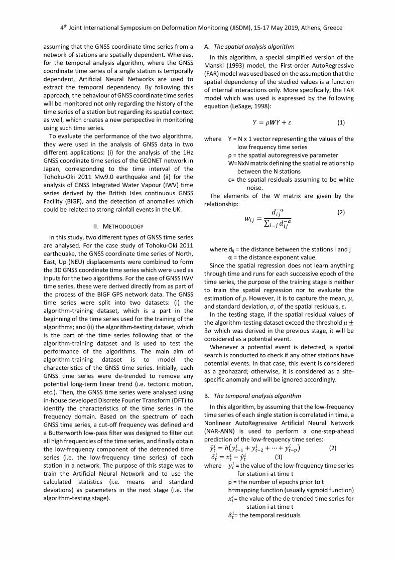
Figure 1: Flowchart of the algorithm-testing stage of the two

algorithms (a) spatial and (b) temporal

Figure 2: Representation of temporal and spatial analysis for a four-station network. The temporal (blue) analysis is done

on the individual time history of each station, whereas spatial (red) analysis runs across the network for each epoch

of the time series.

The predicted value of the low-frequency time series of each station is a function of its previous values only (𝑦7+:: 𝑎𝑛𝑑𝑦7+;: ). This function is estimated by training the NAR-ANN (Eq.2) by using the algorithm-training dataset (Hagan et al., 1996). The temporal residual,𝛿7:, is calculated as the difference between the value of the de-trended time series (e.g.𝑥7:) and the predicted values of 𝑦7: (i.e. 𝑦7:D) which includes all high-frequency components and the abnormalities that the NAR-ANN could not predicts. Finally, calculating the mean and standard deviation of the temporal residuals is used in estimating 𝜇 ± 3𝜎 thresholds.

In the testing stage, the trained NAR-ANN is used to perform a one-step-ahead prediction of the low-frequency time series. If the temporal residual value is beyond the threshold derived in the algorithm-training stage, it will be considered as a potential event (Figure 3b).

III. CASE STUDY: TOHOKU OKI 2011 EARTHQUAKE

The Tohoku-Oki Mw9.0 earthquake occurred at 05:46:23 UTC on March 11th 2011and it was recorded by the GEONET network of GNSS stations operated by the Geospatial Information Authority of Japan (GSI) and numerous studies have been made using the GNSS network data to demonstrate the application of GPS in EEW systems and estimate the strong for the determination of the fault model and earthquake characteristics (Ohta et al., 2012; Colombelli et al., 2013; Psimoulis et al., 2015; Psimoulis et al., 2018). In this case study, the performance of the two algorithms was examined for a six-hour time period of GPS records, covering the earthquake occurrence.

A. Available Data

The 1Hz GPS data of 847 stations from the GEONET network were processed using Bernese software 5.2 and resulted in the GNSS coordinate time series of North, East, Up (NEU) displacements with respect to reference coordinates. For the purpose of this study, the GNSS coordinate time series were combined to form GNSS coordinate time series of 3D displacements (Fig. 3). The GPS time series covered a period of 5 hours and 47 minutes before and 1 hour after the earthquake. B. Analysis of GPS data

The 1Hz GNSS coordinate time series were split in the algorithm-training dataset (5 hours and 40 minutes) followed by the algorithm-testing dataset (12 minutes corresponding to 7 and 5 minutes before and after the earthquake). Regarding the spatial analysis, where the spatial weights matrix derives from the geometry of the GNSS network stations two solutions were examined: (i) one using the entire GPS network and (ii) one using a limited number of stations by ignoring any stations that are located farther than a cap distance. In this study, the cap distance of 200 km is presented and the distance


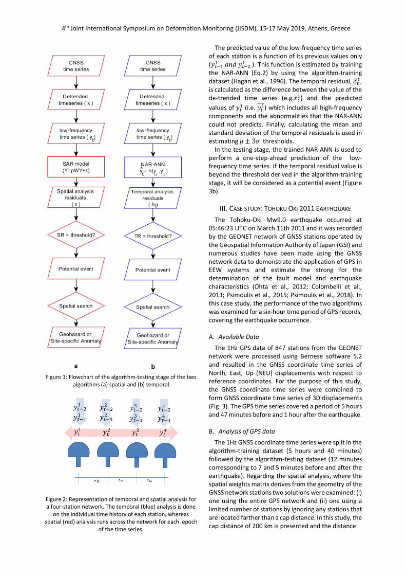
Figure 3. The GPS co-seismic displacement of the Tohoku-Oki

Mw9.0 2011 earthquake.

exponent value α was defined equal to 2, as this combination proved to have the best outcome. Furthermore, for the spatial search, using a search distance of 50 km is effectively used as 96% of the GPS stations are surrounded by at least three other stations.

C. Results

The temporal analysis proved to be highly sensitive and has a consistent result with the study by Psimoulis et al. (2018b), which was based on a similar approach, without though applying the ANN-NAR method. However, due to the limited GPS records duration, there is no evident benefit from the application of ANN-NAR, as there is no significant contribution of the long-period impact in the GPS time-series. Regarding the spatial analysis approach, by using the entire network, it is observed unrealistic early detection of the seismic signal at GPS sites far from the epicentre and this is due to the significant influence of the large displacement of GPS sites close to the epicentre (even up to a few m), across the GPS network. However, by applying the cap distance factor, this influence is limited only to surrounding stations, allowing for a more realistic detection of the seismic signal across the GPS network. However, the detection by using the spatial analysis is still slower than that of temporal analysis.

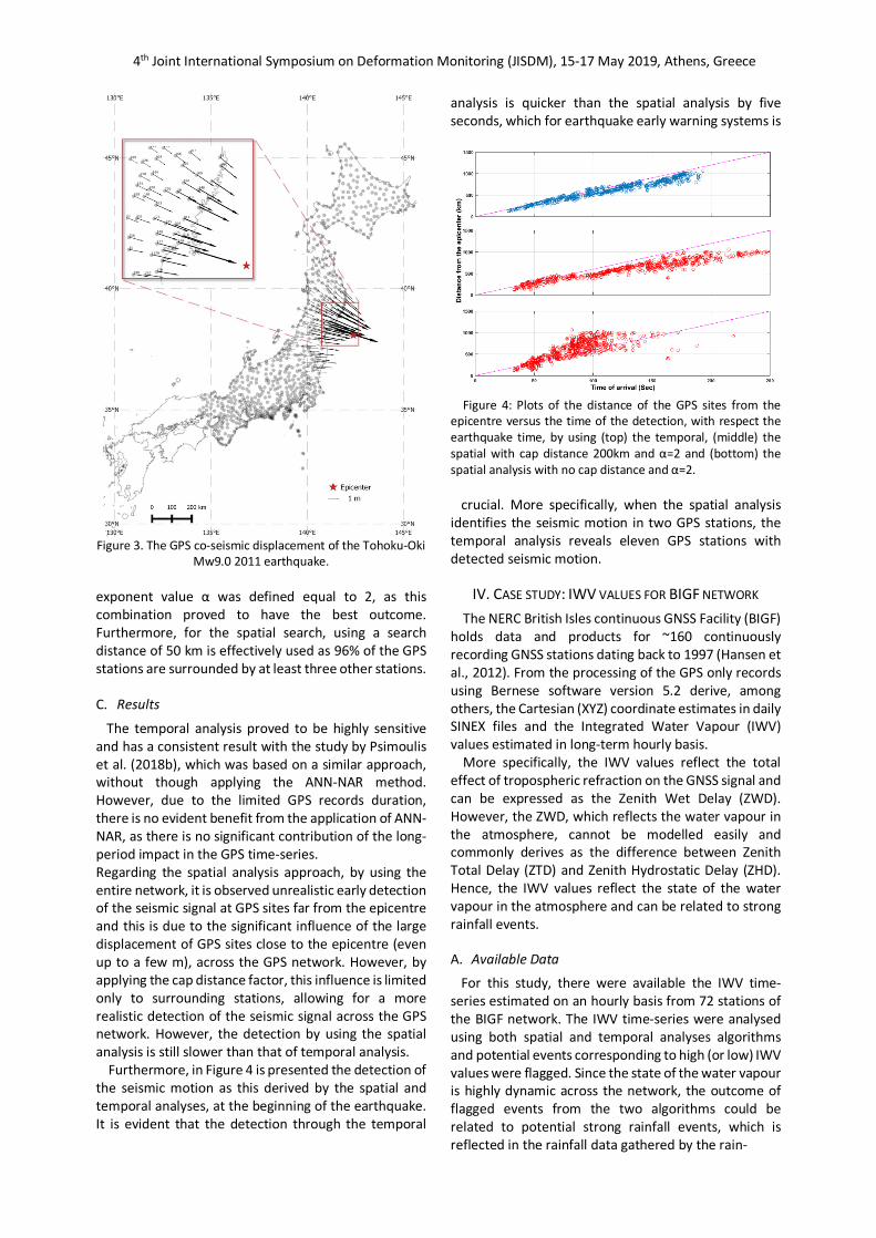
Furthermore, in Figure 4 is presented the detection of the seismic motion as this derived by the spatial and temporal analyses, at the beginning of the earthquake. It is evident that the detection through the temporal

analysis is quicker than the spatial analysis by five seconds, which for earthquake early warning systems is

Figure 4: Plots of the distance of the GPS sites from the

epicentre versus the time of the detection, with respect the earthquake time, by using (top) the temporal, (middle) the spatial with cap distance 200km and α=2 and (bottom) the spatial analysis with no cap distance and α=2.

crucial. More specifically, when the spatial analysis

identifies the seismic motion in two GPS stations, the temporal analysis reveals eleven GPS stations with detected seismic motion.

IV. CASE STUDY: IWV VALUES FOR BIGF NETWORK

The NERC British Isles continuous GNSS Facility (BIGF) holds data and products for ~160 continuously recording GNSS stations dating back to 1997 (Hansen et al., 2012). From the processing of the GPS only records using Bernese software version 5.2 derive, among others, the Cartesian (XYZ) coordinate estimates in daily SINEX files and the Integrated Water Vapour (IWV) values estimated in long-term hourly basis.

More specifically, the IWV values reflect the total effect of tropospheric refraction on the GNSS signal and can be expressed as the Zenith Wet Delay (ZWD). However, the ZWD, which reflects the water vapour in the atmosphere, cannot be modelled easily and commonly derives as the difference between Zenith Total Delay (ZTD) and Zenith Hydrostatic Delay (ZHD). Hence, the IWV values reflect the state of the water vapour in the atmosphere and can be related to strong rainfall events.

A. Available Data

For this study, there were available the IWV time-series estimated on an hourly basis from 72 stations of the BIGF network. The IWV time-series were analysed using both spatial and temporal analyses algorithms and potential events corresponding to high (or low) IWV values were flagged. Since the state of the water vapour is highly dynamic across the network, the outcome of flagged events from the two algorithms could be related to potential strong rainfall events, which is reflected in the rainfall data gathered by the rain-


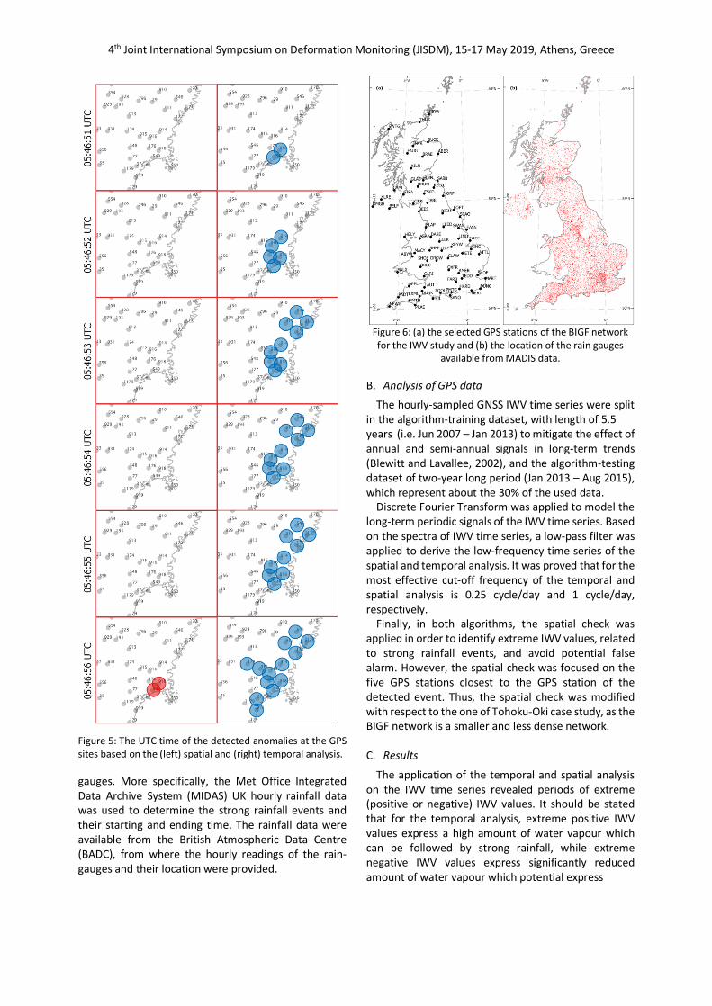
Figure 5: The UTC time of the detected anomalies at the GPS sites based on the (left) spatial and (right) temporal analysis.

gauges. More specifically, the Met Office Integrated Data Archive System (MIDAS) UK hourly rainfall data was used to determine the strong rainfall events and their starting and ending time. The rainfall data were available from the British Atmospheric Data Centre (BADC), from where the hourly readings of the rain-gauges and their location were provided.

Figure 6: (a) the selected GPS stations of the BIGF network for the IWV study and (b) the location of the rain gauges

available from MADIS data.

B. Analysis of GPS data

The hourly-sampled GNSS IWV time series were split in the algorithm-training dataset, with length of 5.5 years (i.e. Jun 2007 – Jan 2013) to mitigate the effect of annual and semi-annual signals in long-term trends (Blewitt and Lavallee, 2002), and the algorithm-testing dataset of two-year long period (Jan 2013 – Aug 2015), which represent about the 30% of the used data.

Discrete Fourier Transform was applied to model the long-term periodic signals of the IWV time series. Based on the spectra of IWV time series, a low-pass filter was applied to derive the low-frequency time series of the spatial and temporal analysis. It was proved that for the most effective cut-off frequency of the temporal and spatial analysis is 0.25 cycle/day and 1 cycle/day, respectively.

Finally, in both algorithms, the spatial check was applied in order to identify extreme IWV values, related to strong rainfall events, and avoid potential false alarm. However, the spatial check was focused on the five GPS stations closest to the GPS station of the detected event. Thus, the spatial check was modified with respect to the one of Tohoku-Oki case study, as the BIGF network is a smaller and less dense network.

C. Results

The application of the temporal and spatial analysis on the IWV time series revealed periods of extreme (positive or negative) IWV values. It should be stated that for the temporal analysis, extreme positive IWV values express a high amount of water vapour which can be followed by strong rainfall, while extreme negative IWV values express significantly reduced amount of water vapour which potential express


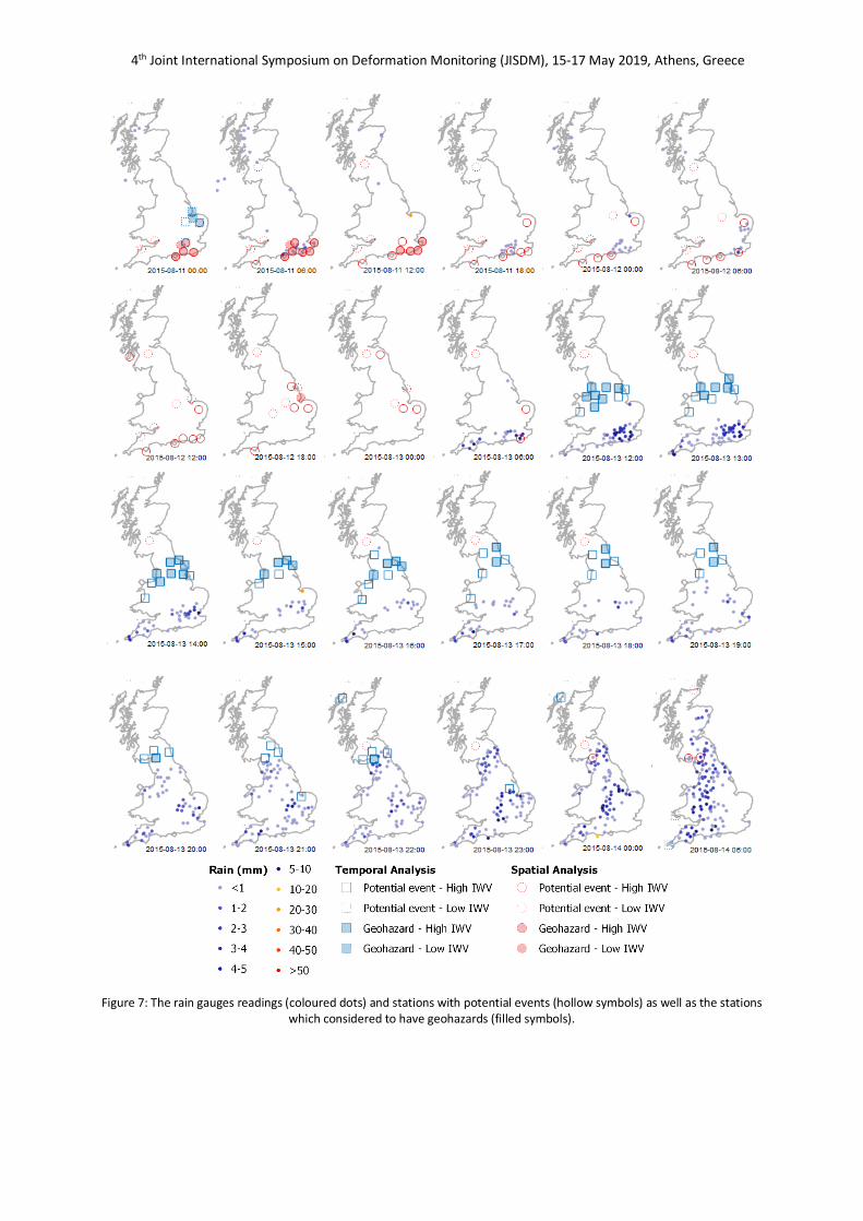
Figure 7: The rain gauges readings (coloured dots) and stations with potential events (hollow symbols) as well as the stations which considered to have geohazards (filled symbols).


significant improvement of the weather after rainfall. The mean value of these temporal residuals thresholds is 8.7 kg.m-2. On the other hand, for the spatial analysis algorithm, the extreme positive or negative IWV values are just relevant to the surrounding GPS stations, expressing a local effect without indicating directly high or low water vapour values. The mean value of these spatial residuals thresholds is 3.0 kg.m-2.

In Figure 7 is presented an indicative example of the flagged event by spatial and temporal analyses algorithms. The spatial algorithm detects a relatively high amount of water vapour accumulated slowly in a period of 18-hours, which is then followed by a local rainfall event. On the contrary, the temporal analysis algorithm flags the locations of a high amount of water vapour, which is moving dynamically and crossing significant part of the network in a few-hour period and then followed by rainfall, as this is indicated by the rain-gauge data.

In general, from the analysis of the temporal analysis algorithm, it was proved that the flagged events express dynamic changes of the water vapour related often with strong rainfall. Furthermore, the locations of the flagged stations change dynamically followed by the rain front. On the contrary, the flagged events from the spatial analysis algorithm reflect the slow accumulation of high amount of water vapour locally in small regions, which remain static and then related to local rainfall events.

V. CONCLUSIONS

Two different algorithms have been developed based on temporal and spatial analyses in order to detect anomalies in GNSS product time series, related to potential geohazards. The developed algorithms were assessed for two case studies of different type of geohazards, differing in scale and severity, and two different types of GNSS network of different size and density. The temporal analysis algorithm seemed to be more efficient for rapidly developed geohazards, as such in the case of the Tohoku-Oki earthquake or the rain front which changes and moves dynamically. On the contrary, the spatial analysis algorithm seems to be more efficient for slowly developed geohazards with regional scale. It was also proved, that the two developed algorithms can be applied in various type of geohazards or type of monitoring data, as in the current study were applied in GPS coordinate and IWV time series. However, the appropriate modifications need to be made based on the type of the monitored data, the type of the network and the monitored geohazard.

VI. ACKNOWLEDGEMENTS

This study was funded by the Dean of Engineering Research Scholarship for International Excellence. The services of the British Isles continuous GNSS Facility (BIGF) in providing archived GNSS products to this study are also gratefully acknowledged.

References Allen, R.M., H. Kanamori, (2003). The Potential for Earthquake

Early Warning in Southern California. Science, Vol. 80, 300 Bevis, M., W., Scherer, M., Merrifield, (2002). Technical Issues

and Recommendations Related to the Installation of Continuous GPS Stations at Tide Gauges, Marine Geodesy, Vol. 25, pp. 87–99

Bhattacharya, D., J.K. Ghosh, N.K. Samadhiya (2012). Review of Geohazard Warning Systems toward Development of a Popular Usage Geohazard Warning Communication System. Natural Hazards Review, Vol 13, pp. 260–271.

Blewitt, G., D., Lavallee, (2002). Effect of annual signals on geodetic velocity, Journal of Geophysical Research: Solid Earth, Vol. 107(7), pp. 9-1 – 9-11.

Blewitt, G., W.C. Hammond, C.Kreemer, H.P. Plag, S. Stein, E. Okal (2009). GPS for real-time earthquake source determination and tsunami warning systems. Journal of Geodesy, Vol. 83, pp. 335–343

Colombelli, S., R.M. Allen, A. Zollo (2013). Application of real-time GPS to earthquake early warning in subduction and strike-slip environments. Journal Geophysical Research: Solid Earth, Vol. 118, pp. 3448–3461.

Crowell, B.W., Y., Bock, Z., Liu, (2016). Single-station automated detection of transient deformation in GPS time series with the relative strength index: A case study of Cascadian slow-slip. Journal of Geophysical Research Solid Earth, Vol. 121(12), 9077-9094.

Edwards, B., B. Allmann, D. F?h, J. Clinton, G. Di Toro, (2010). Automatic computation of moment magnitudes for small earthquakes and the scaling of local to moment magnitude. Geophysical Journal International, Vol. 183, pp. 407–420.

Houlié, N., P. Briole, A. Bonforte, G. Puglisi, (2006). Large scale ground deformation of Etna observed by GPS between 1994 and 2001. Geophysical Research Letters, Vol. 33.

Malet, J.-P., O., Maquaire, E., Calais (2002). The use of Global Positioning System techniques for the continuous monitoring of landslides: application to the Super-Sauze earthflow (Alpes-de-Haute-Provence, France), Geomorphology, 43, 33–54.

Manski, C.F., (1993). Identification of Endogenous Social Effects: The Reflection Problem. Rev. Econ. Stud. Vol. 60, pp. 531–542

Melgar, D., B.W., Crowell, Y. Bock, J.S. Haase (2013). Rapid modeling of the 2011 Mw 9.0 Tohoku-oki earthquake with seismogeodesy. Geophysical Research Letters, Vol. 40, pp. 2963–2968.

Melgar, D., B.W., Crowell, J. Geng, R.M., Allen, Y., Bock, S., Riquelme, E.M., Hill, M., Protti, A., Ganas (2015). Earthquake magnitude calculation without saturation from the scaling of peak ground displacement. Geophysical Research Letter, Vol. 42(13), 5197-5205.

Newman, A. V., S. Stiros, L. Feng, P. Psimoulis, F. Moschas, V. Saltogianni, Y. Jiang, C. Papazachos, D. Panagiotopoulos, E. Karagianni, D. Vamvakaris (2012). Recent geodetic unrest at Santorini Caldera, Greece. Geophysical Research Letters, Vol. 39, n/a-n/a.

Ohta, Y., T. Kobayashi, H. Tsushima, S. Miura, R. Hino, T. Takasu, H. Fujimoto, T. Iinuma, K. Tachibana, T. Demachi, T. Sato, M. Ohzono, N. Umino (2012). Quasi real-time fault model estimation for near-field tsunami forecasting based

4th Joint International Symposium on Deformation Monitoring (JISDM), 15-17 May 2019, Athens, Greece on RTK-GPS analysis: Application to the 2011 Tohoku-Oki earthquake ( M w 9.0). Journal Geophysical Research: Solid Earth, Vol. 117, n/a-n/a.

Psimoulis, P.A., N. Houlié, C. Michel, M. Meindl, M. Rothacher (2014). Long-period surface motion of the multipatch Mw9.0 Tohoku-Oki earthquake. Geophysical Journal International, Vol. 199, pp. 968–980.

Psimoulis, P.A., N. Houlié, Y., Behr, (2018a). Real-time magnitude characterization of large earthquakes using the predominant period derived from 1 Hz GPS data, Geophysical Research Letters, Vol. 45(2), pp. 517-526.

Psimoulis, P.A., N. Houlié, M. Habboub, C. Michel, M. Rothacher (2018b). Detection of ground motions using high-rate GPS time-series. Geophysical Journal International, Vol. 214(2), pp. 1218–1236.

Teferle, F.N., R.M., Bingley, S.D.P., Williams, T.F., Baker, A.H., Dodson, (2006). Using continuous GPS and absolute gravity to separate vertical land movements and changes in sea-level at tide-gauges in the UK. Philos. Trans. A. Math. Phys. Eng. Sci. Vol. 364, pp. 917–930

Wright, T.J., N. Houlié, M. Hildyard, T. Iwabuchi (2012). Real-time, reliable magnitudes for large earthquakes from 1 Hz GPS precise point positioning: The 2011 Tohoku-Oki (Japan) earthquake. Geophysical Research Letters Vol. 39, n/a-n/a

Documents

Temporal and Spatial Analysis of GNSS network data for