Embed Size (px)
Citation preview

Templates and Detection
CSE 4310 – Computer VisionVassilis Athitsos
Computer Science and Engineering DepartmentUniversity of Texas at Arlington

2
The Detection Problem• One can define the detection problem in
various ways.• In this class, the detection problem is the
problem of finding the bounding boxes where some specific type of object appears in an image.
• Example: face detection.– Find the bounding boxes of faces.
• Note: we do not know how many times the type of object we are looking for appears in the image.– Can be zero, one, multiple times.– For example, for face detection, the input
image may have zero, one, or multiple faces.
3
What is a Template?
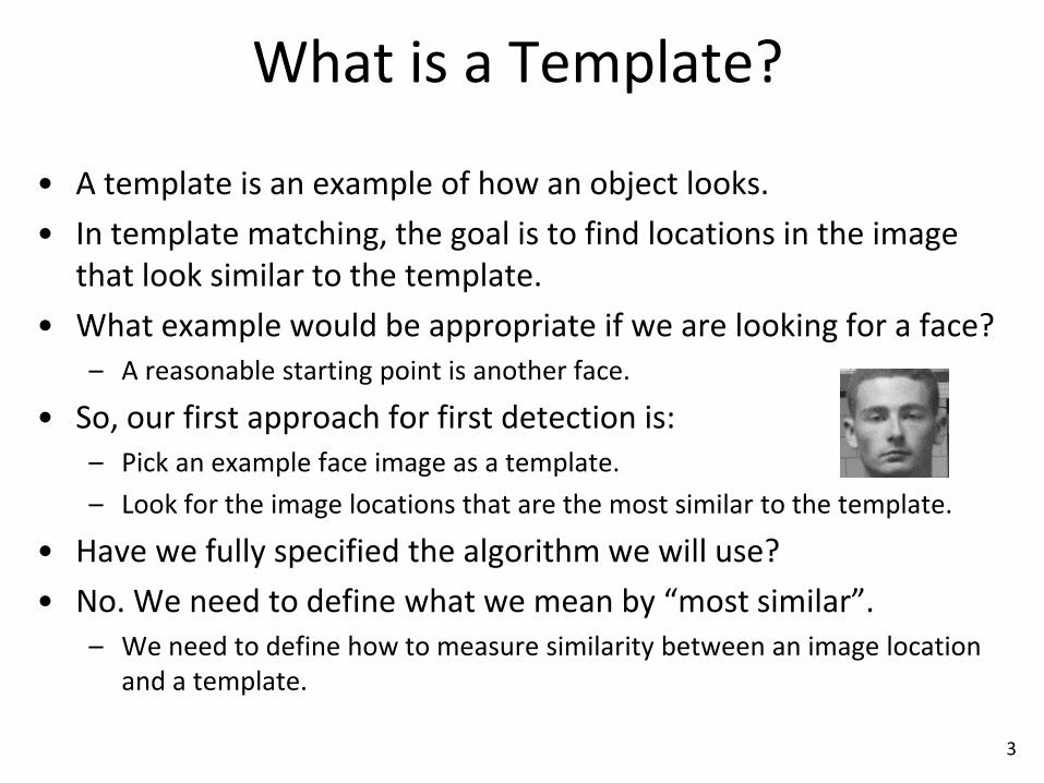
• A template is an example of how an object looks.• In template matching, the goal is to find locations in the image
that look similar to the template.• What example would be appropriate if we are looking for a face?
– A reasonable starting point is another face.
• So, our first approach for first detection is:– Pick an example face image as a template.– Look for the image locations that are the most similar to the template.
• Have we fully specified the algorithm we will use?• No. We need to define what we mean by “most similar”.
– We need to define how to measure similarity between an image location and a template.

4
Sum of Squared Differences
• A simple way to measure similarity is using sums of squared differences (SSD) between each image subwindow and the template.
• First, let’s define the SSD between two vectors.• Let 𝑣𝑣,𝑤𝑤 be 𝐷𝐷-dimensional vectors. 𝑣𝑣 = 𝑣𝑣1,𝑣𝑣2, … , 𝑣𝑣𝐷𝐷 , 𝑤𝑤 = 𝑤𝑤1,𝑤𝑤2, … ,𝑤𝑤𝐷𝐷
• The sum of squared differences SSD 𝑣𝑣,𝑤𝑤 is defined as:
SSD 𝑣𝑣,𝑤𝑤 = �𝑑𝑑=1
𝐷𝐷
𝑣𝑣𝑑𝑑 − 𝑤𝑤𝑑𝑑 2

5
Defining Similarity Using SSD• To find the image subwindow that is the most similar to the
template, we need to measure the SSD between each subwindowand the template.– We define a function ssd_scores(image, template).– This function returns a result of the same size as the image.– result(i,j) is the sum of squared differences between the template and the
image subwindow centered at (i,j).– Specifically, if the template has R rows and C columns (R, C should be odd):
result 𝑖𝑖, 𝑗𝑗 = �𝑟𝑟=1
𝑅𝑅
�𝑐𝑐=1
𝐶𝐶
image 𝑖𝑖 −𝑅𝑅2
+ 𝑟𝑟, 𝑗𝑗 −𝐶𝐶2
+ 𝑐𝑐 − template 𝑟𝑟, 𝑐𝑐2
– We can ignore boundary pixels (i,j), where no full R × 𝐶𝐶 image subwindowcentered at (i,j) can be extracted.
• Good matches correspond to low SSD scores.

6
SSD Pseudocode• Input arguments: grayscale image, template.• result = 2D array of the same size as the image.• Initialize all values of result to -1.• For every location (i,j) in image.
– window = image subwindow centered at (i,j), of same size as the template.– window_vector = window(:) % vector containing the values of window– template_vector = template(:) % vector containing the values of template– diff_vector = window_vector – template_vector– squared_diffs = diff_vector .* diff_vector– ssd_score = sum(squared_diffs)– result(i,j) = ssd_score
• Return result

7
Comments on Pseudocode• In the pseudocode we just saw, the result array has these values:
– Boundary pixels (where we could not extract a valid subwindow of the same size as the template) receive values of -1.
– Interior pixels receive SSD scores.
• The caller function will typically look for the lowest scores in the result, since lowest scores correspond to best matches with the template.– The caller function should ignore boundary values when looking for lowest
scores. We mark those values with -1, to make them easy to identify.
• Obviously, your code can use different conventions to mark invalid scores in boundary pixels. The pseudocode just provides an example of how to handle this issue.– It is important to emphasize, though, that we should always be careful
about marking valid and invalid values in our result images.

8
A Good Result Using SSD Scores
template
input image
SSD scores window with lowest score

9
A Bad Result Using SSD Scores
template
input image
SSD scores window with lowest score

10
Some Obvious Shortcomings• The face detection method we have just outlined is extremely
simple.• There are some obvious shortcomings.• Can you think of cases where this method would be rather
unlikely to succeed?• Here is a summary of shortcomings.
– This method works if the face in the image has similar brightness and contrast as the face in the template. We will fix this.
– This method works if the face in the image has the same size as the face in the template. We will fix this.
– This method works if the face in the image is rotated in the same way as the face in the template. We will partially fix this.
– This method works if the face in the image is fully visible. We will NOT fix this (at least not using templates).

11
Brightness Variations
input image(originalversion)
window with lowest score
input image(brighter version)
window with lowest score

12
Brightness Variations and SSD• Changing the brightness changes the SSD scores.
diff_vector = subwindow_ij(:) – template(:)result(i,j) = sum(diff_vector .* diff_vector)
• If the face subwindow is substantially brighter or darker than the template, the SSD score will be high.
• In some cases, we are OK with that.– If we are confident that the template and its match in the
image should be similarly bright, then we DO want to penalize windows that are much brighter or darker than the template.
• In other cases (like generic face detection) we want to tolerate changes in brightness.

13
Solution: Normalize For Brightness• We can subtract from every window its average intensity value.
– Then, the average intensity value of all windows will be 0.
• For this to work correctly:– The template is normalized, by subtracting from it its average intensity.
template = template – mean(template(:))
– Each image subwindow is normalized, by subtracting from it its average intensity, right before measuring its SSD with the (normalized) template.
subwindow_ij = subwindow_ij – mean(subwindow_ij(:))diff_vector = subwindow_ij(:) – template(:)result(i,j) = sum(diff_vector .* diff_vector)
• DO NOT simply normalize the entire input image in a single step.– We want each individual window to have a mean brightness of 0.

14
Result
input image(brighter version)
window with lowest SSD score
window with lowest SSD score using brightness normalization

15
Contrast
• The brightness of a region corresponds to the average of the intensity values in that region.
• The contrast of a region corresponds to the standard deviation of the intensity values in that region.
• High contrast regions are regions whose intensity values have high standard deviation.– Many pixels significantly brighter than the average within that
region.– Many pixels significantly darker than the average within that
region.

16
Examples of High and Low Contrast
• The left image has higher contrast than the right image.• Both of them have the same average intensity.• Obviously, lower contrast makes some details harder to
see.
17
Results with High and Low Contrast
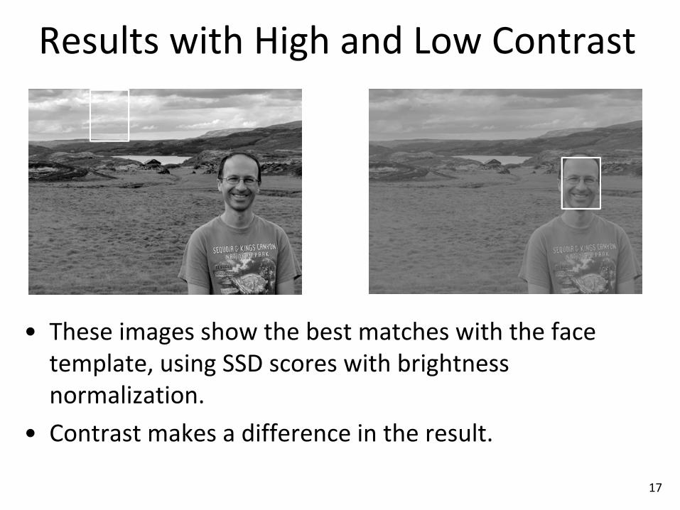
• These images show the best matches with the face template, using SSD scores with brightness normalization.
• Contrast makes a difference in the result.

18
Solution: Normalize for Contrast
• Brightness normalization: we subtract from every window its average intensity value.– Then, the average intensity value of all windows will be 0.
• Contrast normalization (done AFTER brightness normalization).– We divide each window by the standard deviation of values in
that window.
• As was the case for brightness normalization:– The template is normalized separately, based on its own mean
and standard deviation.– Each image subwindow is normalized separately, based on its
own mean and standard deviation.

19
Normalization Code• The template is normalized at the beginning.
% normalize template for brightnesstemplate = template – mean(template(:))% normalize template for contrasttemplate = template / std(template(:))
• Each image subwindow is normalized, right before measuring its SSD with the (normalized) template.
% normalize subwindow for brightnesssubwindow_ij = subwindow_ij – mean(subwindow_ij(:))% normalize subwindow for contrastsubwindow_ij = subwindow_ij / std(subwindow_ij(:))diff_vector = subwindow_ij(:) – template(:)result(i,j) = sum(diff_vector .* diff_vector)

20
Results After Brightness and Contrast Normalization

21
Normalized Cross-correlation
• Let 𝑣𝑣,𝑤𝑤 be 𝐷𝐷-dimensional vectors. 𝑣𝑣 = 𝑣𝑣1,𝑣𝑣2, … , 𝑣𝑣𝐷𝐷 , 𝑤𝑤 = 𝑤𝑤1,𝑤𝑤2, … ,𝑤𝑤𝐷𝐷
• Let 𝜇𝜇𝑣𝑣 and 𝜇𝜇𝑤𝑤 be the means of 𝑣𝑣 and 𝑤𝑤:
𝜇𝜇𝑣𝑣 = ∑𝑑𝑑=1𝐷𝐷 𝑣𝑣𝑑𝑑𝐷𝐷
, 𝜇𝜇𝑤𝑤 = ∑𝑑𝑑=1𝐷𝐷 𝑤𝑤𝑑𝑑𝐷𝐷
• Let 𝜎𝜎𝑣𝑣 and 𝜎𝜎𝑤𝑤 be the standard deviations of 𝑣𝑣 and 𝑤𝑤:
𝜎𝜎𝑣𝑣 = ∑𝑑𝑑=1𝐷𝐷 𝑣𝑣𝑑𝑑−𝜇𝜇𝑣𝑣 2
𝐷𝐷−1, 𝜎𝜎𝑤𝑤 = ∑𝑑𝑑=1
𝐷𝐷 𝑤𝑤𝑑𝑑−𝜇𝜇𝑤𝑤 2
𝐷𝐷−1
• The normalized cross-correlation C 𝑣𝑣,𝑤𝑤 is defined as:
C 𝑣𝑣,𝑤𝑤 =∑𝑑𝑑=1𝐷𝐷 𝑣𝑣𝑑𝑑 − 𝜇𝜇𝑣𝑣 𝑤𝑤𝑑𝑑 − 𝜇𝜇𝑤𝑤
𝜎𝜎𝑣𝑣𝜎𝜎𝑤𝑤

22
Normalized Cross-correlation
• The normalized cross-correlation C 𝑣𝑣,𝑤𝑤 is defined as:
C 𝑣𝑣,𝑤𝑤 =∑𝑑𝑑=1𝐷𝐷 𝑣𝑣𝑑𝑑 − 𝜇𝜇𝑣𝑣 𝑤𝑤𝑑𝑑 − 𝜇𝜇𝑤𝑤
𝜎𝜎𝑣𝑣𝜎𝜎𝑤𝑤
• The normalized cross correlation can be interpreted as the dot product of two unit vectors:– First unit vector: 𝑣𝑣−𝜇𝜇𝑣𝑣
𝜎𝜎𝑣𝑣
– Second unit vector: 𝑤𝑤−𝜇𝜇𝑤𝑤𝜎𝜎𝑤𝑤
• Note: 𝜎𝜎𝑣𝑣 is the norm of 𝑣𝑣 −𝜇𝜇𝑣𝑣, 𝜎𝜎𝑤𝑤 is the norm of 𝑤𝑤 −𝜇𝜇𝑤𝑤.

23
Normalized Cross-correlation
• The normalized cross-correlation C 𝑣𝑣,𝑤𝑤 is defined as:
C 𝑣𝑣,𝑤𝑤 =∑𝑑𝑑=1𝐷𝐷 𝑣𝑣𝑑𝑑 − 𝜇𝜇𝑣𝑣 𝑤𝑤𝑑𝑑 − 𝜇𝜇𝑤𝑤
𝜎𝜎𝑣𝑣𝜎𝜎𝑤𝑤• Properties of normalized cross-correlation C 𝑣𝑣,𝑤𝑤 :
– Highest possible value: 1• C 𝑣𝑣, 𝑣𝑣 = 1
– Lowest possible value: -1• C 𝑣𝑣,−𝑣𝑣 = 1
– Higher values indicate higher similarity between 𝑣𝑣 and 𝑤𝑤.
• If 𝑣𝑣,𝑤𝑤 are unit vectors, then C 𝑣𝑣,𝑤𝑤 = 1 − 𝑣𝑣 − 𝑤𝑤 2.– The lower the Euclidean distance, the higher the correlation.

24
Normalized Cross-correlation• Normalized cross-correlation provides an alternative way to find
matches of a template with an image.– Instead of looking for lowest SSD score, we look for highest normalized
cross-correlation score.
• The detection results we get with normalized cross-correlation are the same as the results we get with SSD, if we use brightness and contrast normalization when measuring SSD.– When we normalize an image window for brightness and contrast, we
convert the window to a unit vector.– Highest cross-correlation scores correspond to lowest SSD scores.
• Mathematically, both approaches are equivalent.

25
Normalized Cross-correlation in Matlab
• In Matlab, there is a built-in function called normxcorr2.• normxcorr2(template, image) returns an array of
normalized cross-correlation scores between the template and each template-sized subwindow of the image.
• However, the result of normxcorr2 does not have the same size as the image.– It includes extra scores in the boundary.

26
Normalized Cross-correlation in Matlab
• In the code posted on the course website, we include a normalized_correlation function, which serves as a convenient wrapper function for normxcorr2.
• normalized_correlation(image, template) returns a result of the same size as the image. result(i,j) is the normalized cross-correlation score between
the template and the template-sized image subwindowcentered at pixel (i,j).
Boundary pixels (where we could not extract a valid subwindow of the same size as the template) receive values of 0.

27
Detection at Different Scales
• This is an example we saw before, where the face is detected successfully.
template

28
Detection at Different Scales
• Here is the result on a 23% smaller version of the image.• The face is now somewhat smaller than the template.• Normalized cross-correlation (same as SSD with
brightness/contrast normalization) cannot handle that.
template
29
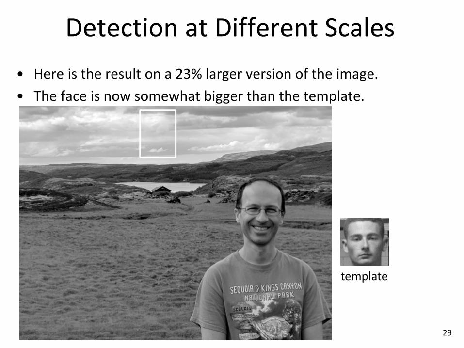
Detection at Different Scales• Here is the result on a 23% larger version of the image.• The face is now somewhat bigger than the template.
template

30
Detection at Different Scales
• SSD and normalized cross-correlation assume that the object that we want to detect is about as large as the template.
• This is too much of a restriction.– Typically we do not know in advance how large or small
objects of interest are in an image.– A detector should be able to detect objects regardless of how
big they appear (unless they appear so small that they cannot be seen clearly).

31
Scaling the Image
• What can we do to detect the face if we know that the face is about three times larger than the template?
template
Original image, face about three timeslarger than in the template.

32
Scaling the Image
• What can we do to detect the face if we know that the face is about three times larger than the template?
• First approach: scale down the image.– Scale the image down by a factor of three.– Get normalized cross-correlation scores between the scaled
down image and the template.• In the scaled-down image, the face is about the same size as the
template.
– Scale up the cross-correlation scores by a factor of three.• So that scores(i,j) corresponds to the subwindow centered at (i,j) in the
original image.
– Find maximum score location in the scaled-up scores.

33
Example
template
Original image, face about three timeslarger than in the template.

34
Example
template
Scaled down image, three time smaller

35
Example
template
Normalized correlation scores between small image and template

36
Example
template
Normalized cross-correlation scores scaled upthree times, so that they match the original image.
37
Example
template
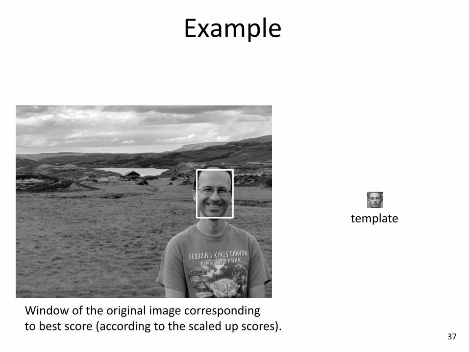
Window of the original image corresponding to best score (according to the scaled up scores).

38
Matlab Code
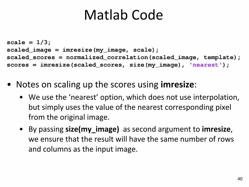
scale = 1/3;scaled_image = imresize(my_image, scale);scaled_scores = normalized_correlation(scaled_image, template);scores = imresize(scaled_scores, size(my_image), 'nearest');
% the rest of the code is just useful for showing the result.max_value = max(scores(:));[rows, cols] = find(scores == max_value);
y = rows(1);x = cols(1);
[template_rows, template_cols] = size(template);face_rows = round(template_rows/scale);face_cols = round(template_cols/scale);result = draw_rectangle2(my_image, y, x, face_rows, face_cols);imshow(result, [0 255]);

39
Matlab Code
scale = 1/3;scaled_image = imresize(my_image, scale);scaled_scores = normalized_correlation(scaled_image, template);scores = imresize(scaled_scores, size(my_image), 'nearest');
• These are the important lines that show how to do template-based face detection if the face is three times larger in the image than on the template.
• Note the three main steps:• Scale down image.• Do normalized correlation of scaled-down image with
template.• Scale up scores, to match the size of the original image.
40
Matlab Code
scale = 1/3;scaled_image = imresize(my_image, scale);scaled_scores = normalized_correlation(scaled_image, template);scores = imresize(scaled_scores, size(my_image), 'nearest');
• Notes on scaling up the scores using imresize:• We use the ‘nearest’ option, which does not use interpolation,
but simply uses the value of the nearest corresponding pixel from the original image.
• By passing size(my_image) as second argument to imresize, we ensure that the result will have the same number of rows and columns as the input image.

41
Alternative: Scaling the Template
• What can we do to detect the face if we know that the face is about three times larger than the template?
• We saw before that we can scale the image down by a factor of three.
• Alternatively???

42
Alternative: Scaling the Template
• What can we do to detect the face if we know that the face is about three times larger than the template?
• We saw before that we can scale the image down by a factor of three.
• Alternatively, we can:– scale up the template by a factor of three.– Get normalized cross-correlation scores between the image
and the scaled-up template.• The face is about the same size as the scaled-up template.
– Find maximum score location in the scores.• No scaling of the scores is needed, since normalized correlation
scores were obtained using the original image.

43
Example
template
Original image, face about three timeslarger than in the template.

44
Example
Original image, face about three timeslarger than in the template.
scaled-uptemplate

45
Example
Normalized cross-correlation scores betweenoriginal image and scaled-up template.
scaled-uptemplate

46
Example
Window of the original image corresponding to best score (according to the scaled up scores).
scaled-uptemplate

47
Matlab Code
scale = 1/3;scaled_template = imresize(template, 1/scale);scores = normalized_correlation(my_image, scaled_template);
% the rest of the code is just useful for showing the result.max_value = max(scores(:));[rows, cols] = find(scores == max_value);
y = rows(1);x = cols(1);
[template_rows, template_cols] = size(template);face_rows = round(template_rows / scale);face_cols = round(template_cols / scale);result = draw_rectangle2(my_image, y, x, face_rows, face_cols);imshow(result, [0 255]);
48
Matlab Code
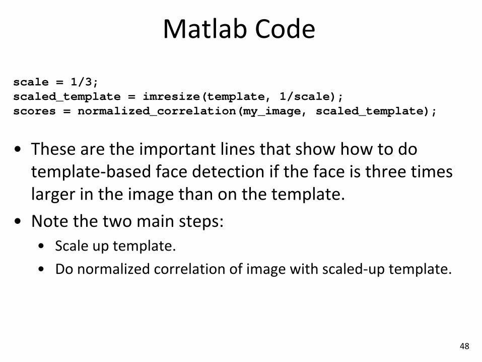
scale = 1/3;scaled_template = imresize(template, 1/scale);scores = normalized_correlation(my_image, scaled_template);
• These are the important lines that show how to do template-based face detection if the face is three times larger in the image than on the template.
• Note the two main steps:• Scale up template.• Do normalized correlation of image with scaled-up template.

49
Multiscale Search
• So, when we know the size of the face (or, more generally, the size of the object to be detected), we can scale the image or the template so that the object in the image matches the size of the template.
• However, typically we do NOT know the size of the object(s) we want to detect.
• What do we do then?• We search at multiple scales.• For each pixel (i,j), we remember:
– The max normalized correlation score it got over all scales.– The scale that produced that max score.

50
Multiscale Search: Matlab Codefunction ...[result, max_scales] = multiscale_correlation(image, template, scales)
result = ones(size(image)) * -10;max_scales = zeros(size(image));
for scale = scales;% for efficiency, we either downsize the image, or the template, % depending on the current scaleif scale >= 1
scaled_image = imresize(image, 1/scale, 'bilinear');temp_result = normalized_correlation(scaled_image, template);temp_result = imresize(temp_result, size(image), 'nearest');
elsescaled_image = image;scaled_template = imresize(template, scale, 'bilinear');temp_result = normalized_correlation(image, scaled_template);
end
higher_maxes = (temp_result > result);max_scales(higher_maxes) = scale;result(higher_maxes) = temp_result(higher_maxes);
end

51
Multiscale Search: Matlab Codefunction ...[result, max_scales] = multiscale_correlation(image, template, scales)
result = ones(size(image)) * -10;max_scales = zeros(size(image));
• We will walk through the implementation of multiscale_correlation, which implements multiscale template search using normalized correlation.
• Arguments:– Image where we want to detect objects.– The template that we want to use.– scales is an array of scales.
• E.g., scales = [0.5, 0.6, 0.7, 0.8, 0.9, 1.0, 1.1, 1.2, 1.3, 1.4, 1.5].

52
Multiscale Search: Matlab Codefunction ...[result, max_scales] = multiscale_correlation(image, template, scales)
result = ones(size(image)) * -10;max_scales = zeros(size(image));
• scales is an array of scales. – E.g., scales = [0.5, 0.6, 0.7, 0.8, 0.9, 1.0, 1.1, 1.2, 1.3, 1.4, 1.5].– Or, equivalently, scales = 0.5:0.1:1.5.
• In the above example, the scales argument only covers scales between 0.5 and 1.5.– Assumes that faces will be between 50% and 150% of the size of the face
template.
• Usually this range is too restrictive, we want a larger range.

53
Multiscale Search: Matlab Codefunction ...[result, max_scales] = multiscale_correlation(image, template, scales)
result = ones(size(image)) * -10;max_scales = zeros(size(image));
The recommended practice for scales is to:• Cover a wide range of scales.
– “Wide range” is not specific enough, but covering scales from 0.1 to 10 is usually a better choice than covering scales from 0.5 to 1.5.
• Use a sequence of scales that increases geometrically, not arithmetically.
• It makes sense to go from scale 0.1 to scale 0.11, because the increase from one scale to the next is about 10%. If anything, this type of gap may be too large in some cases.
• However, going from scale 10.00 to scale 10.01 is usually too conservative, as the increase is only 0.1%, which is needlessly small.

54
Multiscale Search: Matlab Code• This sample code generates a “reasonable” value for the scales
argument, given a smallest scale, largest scale, and ratio of 1.1 between two consecutive values.– Remember, though, what is “reasonable” depends on the application and
the data.
low_scale = 0.1;high_scale = 10;step_ratio = 1.1;ratio = high_scale / low_scale;number_of_steps = ceil(log(ratio)/log(step_ratio));scales = low_scale * (step_ratio .^ (0:number_of_steps));
• The above code generates an array scales of size 50.
scales = [0.10, 0.11, 0.121, 0.133, 0.146, …,7.29, 8.02, 8.82, 9.70, 10.67]
55
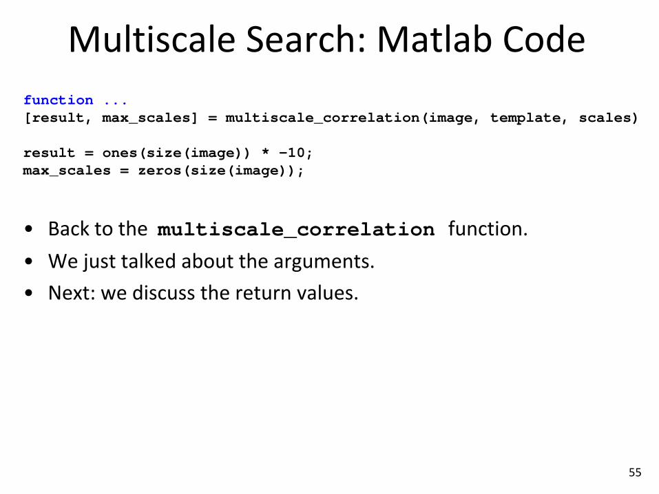
Multiscale Search: Matlab Codefunction ...[result, max_scales] = multiscale_correlation(image, template, scales)
result = ones(size(image)) * -10;max_scales = zeros(size(image));
• Back to the multiscale_correlation function.• We just talked about the arguments.• Next: we discuss the return values.

56
Multiscale Search: Matlab Codefunction ...[result, max_scales] = multiscale_correlation(image, template, scales)
result = ones(size(image)) * -10;max_scales = zeros(size(image));
• Return values.– result(i,j) will store the maximum normalized correlation score found for
location (i,j) over all scales that we try.– max_scales(i,j) will store the scale that produced that maximum
normalized correlation score for location (i,j).
• What value is each result(i,j) initialized to, and why?

57
Multiscale Search: Matlab Codefunction ...[result, max_scales] = multiscale_correlation(image, template, scales)
result = ones(size(image)) * -10;max_scales = zeros(size(image));
• Return values.– result(i,j) will store the maximum normalized correlation score found for
location (i,j) over all scales that we try.– max_scales(i,j) will store the scale that produced that maximum
normalized correlation score for location (i,j).
• What value is each result(i,j) initialized to, and why?– result(i,j) is initialized to -10.– Since result(i,j) will store a maximum normalized correlation value, whose
range is between -1 and 1, it can be initialized to any value less than -1.

58
Multiscale Search: Matlab Code...for scale = scales;
if scale >= 1scaled_image = imresize(image, 1/scale, 'bilinear');temp_result = normalized_correlation(scaled_image, template);temp_result = imresize(temp_result, size(image), 'nearest');
elsescaled_image = image;scaled_template = imresize(template, scale, 'bilinear');temp_result = normalized_correlation(image, scaled_template);
end...
• Note how we do the scaling.– For scales greater than 1 (meaning that the object is larger than the
template), we scale down the image, instead of scaling up the template.– For scales smaller than 1 (meaning that the object is smaller than the
template), we scale down the template, instead of scaling up the image.
• We prefer scaling down over scaling up, for efficiency.

59
Multiscale Search: Matlab Code...
higher_maxes = (temp_result > result);max_scales(higher_maxes) = scale;result(higher_maxes) = temp_result(higher_maxes);
...
• temp_result: normalized correlation scores for current scale.• result(i,j): maximum score found so far for (i,j).• max_scales(i,j): the scale that gave the maximum score for (i,j).• higher_maxes(i,j) is a boolean, indicating if temp_result(i,j) (the
score at the current scale) is larger than result(i,j) (the best score found before the current scale). – If higher_maxes(i,j) is true, we must update result(i,j) and max_scales(i,j).
• The next two lines update the values in the locations of max_scales and result that need to be updated.

60
Using Multiscale Search• This code calls multiscale_correlation and draws the bounding
box of the best matching location (at the right scale).
scales = make_scales_array(0.25, 4, 1.1);
[scores, max_scales] = multiscale_correlation(photo, template, scales);max_score = max(scores(:));[rows, cols] = find(scores == max_score);y = rows(1);x = cols(1);scale = max_scales(y, x);[template_rows, template_cols] = size(template);face_rows = round(template_rows * scale);face_cols = round(template_cols * scale);
result = draw_rectangle2(photo, y, x, face_rows, face_cols);imshow(result, [0 255]);

61
Some Results of Multiscale Search
scales = make_scales_array(0.2, 5, 1.1);scale of highest score: 0.354

62
Some Results of Multiscale Search
scales = make_scales_array(0.2, 5, 1.1);scale of highest score: 2.17

63
Some Results of Multiscale Search
scales = make_scales_array(0.2, 5, 1.1);scale of highest score: 0.22
Obviously, this is the wrong result.Searching over multiple scales, there are more potential false matches.
64
Rotations
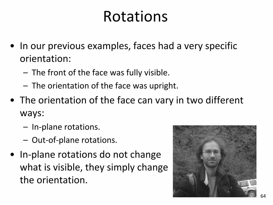
• In our previous examples, faces had a very specific orientation:– The front of the face was fully visible.– The orientation of the face was upright.
• The orientation of the face can vary in two different ways:– In-plane rotations.– Out-of-plane rotations.
• In-plane rotations do not change what is visible, they simply changethe orientation.
65
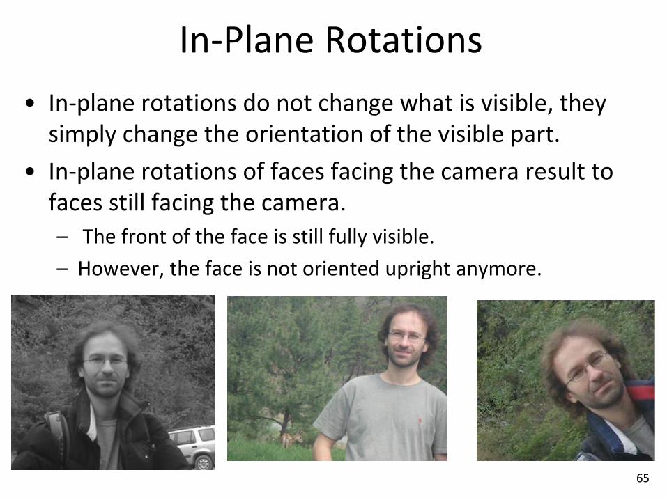
In-Plane Rotations• In-plane rotations do not change what is visible, they
simply change the orientation of the visible part.• In-plane rotations of faces facing the camera result to
faces still facing the camera.– The front of the face is still fully visible.– However, the face is not oriented upright anymore.

66
Out-of-Plane Rotations
• In out-of-plane rotations, the object rotates in a way that changes what is visible.
• If we start with a face whose front is visible, an out-of-plane rotation results to part of the front (or the entire front) not being visible.– Other parts become visible, like side/top/back of head.

67
Handling Rotations
• Handling in-plane rotations can be done similar to the way we handled multiple scales:– Search at multiple rotations, keep track at each location of the
rotation that gives the highest score.– We can rotate the image, or we can rotate the template.– In Matlab, imrotate can be used to do the rotations.
• However, we must be careful of some practical details:– If we rotate the image, and get normalized cross-correlation
scores, we should make sure we know what original image locations those scores correspond to.
– If we rotate the template, we may lose parts of it, or introduce new parts, that may change the correlation scores.

68
Handling Rotations
• Out-of-plane rotations cannot be handled, unless we have templates matching those rotations.– Note that we did not need new templates to handle different
scales or different in-plane rotations.
• For example, to detect faces seen at profile orientation, we should use templates corresponding to profile orientation as well.
• In this course, we will not worry about handling out-of-plane rotations.

69
Number of Detection Results
• In our examples so far, we have computed scores at all image locations (and possibly at multiple scales/orientations), and then shown the best score.
• However, we typically do not know how many objects we should detect.
• We need an automatic way to decide the number of detections.
• Standard approach:– Set a threshold on the score.– Any score above the threshold qualifies as a detection.
• With one exception…

70
Non-Maxima Suppression• Here is an example result that we have seen before.

71
Non-Maxima Suppression• And here is the normalized cross-correlation result on that image.
– Where do you think the second highest score is?

72
Non-Maxima Suppression• And here is the normalized cross-correlation result on that image.
– Where do you think the second highest score is?– Right next to the highest score.

73
Non-Maxima Suppression• If we want to produce multiple (and meaningful) detection
results, we need to suppress results that are almost identical to other results.– We call this operation non-maxima suppression.

74
Non-Maxima Suppression
• Returning multiple results while performing non-maxima suppression of detection results is pretty simple.
• Let T be a detection threshold.• Pseudocode:
– Let S = normalized cross-correlation scores (optionally at multiple scales, rotations, etc).
– detection_locations = [] // empty list– While (true)
• Let s be the max value in S, and let (i,j) be the pixel location of s in S.• If s < T, break.• Insert (i,j) as an element to detection_locations.• Zero out an area of S centered at (i,j). How big this area should be is an
implementation choice. For example, it can be the size of the template.
75
Using Average Images as Templates
• In our examples, we used a face image as a template, to detect other faces.
• However, using a specific face may be problematic.– Some faces may work better than others.
• A common approach is to use an average image as a template.
• An average image is (as the name indicates) the average of multiple images.

76
Computing an Average Face• We need aligned face images:• In this case, aligned means:
– same size– significant features (eyes, nose, mouth), to the degree
possible, are in similar pixel locations.
an example set of aligned face images

77
Result: Average Face

78
Cropping
• It may be beneficial to crop a template, so that we keep the parts of it that are most likely to be present in the image:– Exclude background.– Exclude forehead (highly variable appearance, due to hair).– Exclude lower chin.
average faceface template
79
Measuring Accuracy• Measuring accuracy is an important part of the daily routine in
computer vision work.• We implement various methods, and variations of those
methods, and we want to see what works best.• However, measuring accuracy is not a trivial process.• Different computer vision tasks (detection, recognition, tracking,
segmentation) have their own conventions, that we will learn when we study each task.
• What should be emphasized from the beginning:– Numbers are meaningless, without a clear explanation of what is being
measured, how it is being measured, and on what data it is being measured.
– For example, a statement that system X is “99% accurate” does not provide any useful information, in the absence of such specifications.

80
Some Standard Steps• In measuring accuracy, we need to specify a test set.
– Accuracy will be measured on images from that set.
• For that set, we need to know the “correct” answers.– So, in addition to images, the test set needs to contain those answers.
• These “correct” answers are called ground truth.• Then, the best possible result for the system we are evaluating
would be to produce answers identical to the ground truth.• In the typical case where the system’s answers are not identical
to the ground truth, we need to define quantitative measures of accuracy, that measure how close the results are to the ground truth.

81
Measuring Detection Accuracy
• Detection is a good task for introducing such concepts.• Measuring detection accuracy is more complicated than
measuring other types of accuracy.

82
Ground Truth Annotations• To measure detection accuracy, we need to use some dataset of
images.• For every image in that dataset, we need annotations that specify:
– How many objects of interest are present.– The bounding box of every object of interest.
• Bounding box placement is not an exact science.– Different people will slightly disagree in
where exactly the corners of the bounding box should be.
• However, establishing some clear guidelines is useful, to maintainconsinstency as much as possible.– Does the box go down to the bottom of the
chin? Up to the top of the forehead?

83
Is a Detection Correct?
• In the image below:– Suppose that the yellow box is the ground truth annotation.– Suppose that the red box is the detection result.– Is that result correct or not?

84
Is a Detection Correct?
• In the image below:– Suppose that the yellow box is the ground truth annotation.– Suppose that the red box is the detection result.– Is that result correct or not?
• It is important to have specific rules, so that evaluation of correctness can be done automatically.
• Standard approach: measure theintersection over union (IoU) scorebetween the detection and the ground truth.

85
Intersection Over Union• Intersection over Union (IoU) is a score that measures
the overlap between two regions A and B.• In our case:
– The first region is the ground truth location of the object of interest.
– The second region is a detected bounding box.
• IoU(A,B) is defined as this ratio:
# of pixels in 𝐴𝐴 ∩ 𝐵𝐵# of pixels in 𝐴𝐴 ∪ 𝐵𝐵
• Remember: 𝐴𝐴 ∩ 𝐵𝐵 is intersection, 𝐴𝐴 ∪ 𝐵𝐵 is union.

86
Computing Intersection Over Union• IoU(A,B) is defined as this ratio:
# of pixels in 𝐴𝐴 ∩ 𝐵𝐵# of pixels in 𝐴𝐴 ∪ 𝐵𝐵
• In our example:– 𝐴𝐴 ∩ 𝐵𝐵 is shown by the green rectangle.– 𝐴𝐴 ∪ 𝐵𝐵 is the union of the yellow region, the red region, and the green rectangle.
87
Intersection Over Union
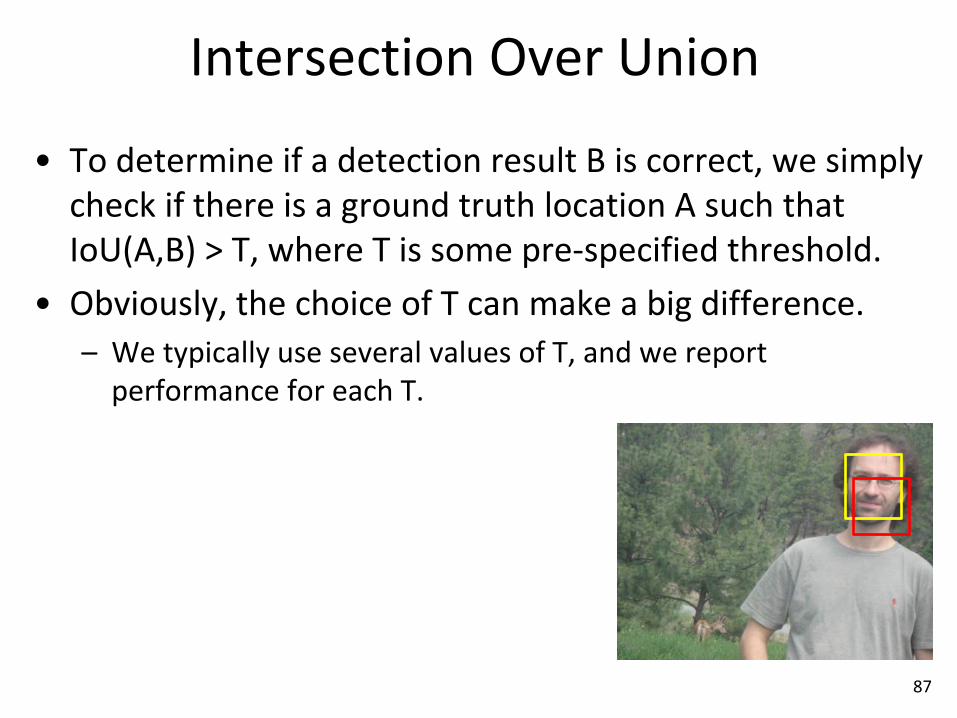
• To determine if a detection result B is correct, we simply check if there is a ground truth location A such that IoU(A,B) > T, where T is some pre-specified threshold.
• Obviously, the choice of T can make a big difference.– We typically use several values of T, and we report
performance for each T.

88
Computing Intersection Over Union• IoU(A,B) is defined as this ratio:
# of pixels in 𝐴𝐴 ∩ 𝐵𝐵# of pixels in 𝐴𝐴 ∪ 𝐵𝐵
• Typically, in evaluating detection accuracy, A and B are rectangles, specified by their top, bottom, left and right coordinates.– A is specified as (𝑇𝑇𝐴𝐴,𝐵𝐵𝐴𝐴, 𝐿𝐿𝐴𝐴,𝑅𝑅𝐴𝐴).– B is specified as (𝑇𝑇𝐵𝐵,𝐵𝐵𝐵𝐵 , 𝐿𝐿𝐵𝐵𝐴𝐴,𝑅𝑅𝐵𝐵).– 𝑇𝑇𝐴𝐴,𝑇𝑇𝐵𝐵 ,𝐵𝐵𝐴𝐴,𝐵𝐵𝐵𝐵 are row numbers.
– 𝐿𝐿𝐴𝐴, 𝐿𝐿𝐵𝐵 ,𝑅𝑅𝐴𝐴,𝑅𝑅𝐵𝐵 are column numbers.
z
𝑇𝑇𝐴𝐴
𝐵𝐵𝐴𝐴
𝑇𝑇𝐵𝐵
𝐵𝐵𝐵𝐵
𝐿𝐿𝐴𝐴𝐿𝐿𝐵𝐵
𝑅𝑅𝐴𝐴
𝑅𝑅𝐵𝐵

89
Computing Intersection Over Union• IoU(A,B) is defined as this ratio:
# of pixels in 𝐴𝐴 ∩ 𝐵𝐵# of pixels in 𝐴𝐴 ∪ 𝐵𝐵
• The rectangle 𝐴𝐴 ∩ 𝐵𝐵, if it is not empty,is specified by these four numbers:
– 𝑇𝑇𝐴𝐴∩𝐵𝐵 = max 𝑇𝑇𝐴𝐴,𝑇𝑇𝐵𝐵– 𝐵𝐵𝐴𝐴∩𝐵𝐵 = min 𝐵𝐵𝐴𝐴,𝐵𝐵𝐵𝐵– 𝐿𝐿𝐴𝐴∩𝐵𝐵 = max 𝐿𝐿𝐴𝐴, 𝐿𝐿𝐵𝐵– 𝑅𝑅𝐴𝐴∩𝐵𝐵 = min 𝑅𝑅𝐴𝐴,𝑅𝑅𝐵𝐵
z
𝐵𝐵𝐴𝐴∩𝐵𝐵
𝑇𝑇𝐴𝐴∩𝐵𝐵
𝐿𝐿𝐴𝐴∩𝐵𝐵
𝑅𝑅𝐴𝐴∩𝐵𝐵

90
Computing Intersection Over Union• IoU(A,B) is defined as this ratio:
# of pixels in 𝐴𝐴 ∩ 𝐵𝐵# of pixels in 𝐴𝐴 ∪ 𝐵𝐵
• The areas of A, B, 𝐴𝐴 ∩ 𝐵𝐵 are computed as:– Height(𝐴𝐴) = 𝐵𝐵𝐴𝐴 − 𝑇𝑇𝐴𝐴 + 1– Width(𝐴𝐴) = 𝑅𝑅𝐴𝐴 − 𝐿𝐿𝐴𝐴 + 1– Area(𝐴𝐴) = Height(𝐴𝐴)* Width(𝐴𝐴)– Height(𝐵𝐵) = 𝐵𝐵𝐵𝐵 − 𝑇𝑇𝐵𝐵 + 1– Width(𝐵𝐵) = 𝑅𝑅𝐵𝐵 − 𝐿𝐿𝐵𝐵 + 1– Area(𝐵𝐵) = Height(𝐵𝐵)* Width(𝐵𝐵)– Height(𝐴𝐴 ∩ 𝐵𝐵) = 𝐵𝐵𝐴𝐴∩𝐵𝐵 − 𝑇𝑇𝐴𝐴∩𝐵𝐵 + 1– Width(𝐴𝐴 ∩ 𝐵𝐵) = 𝑅𝑅𝐴𝐴∩𝐵𝐵 − 𝐿𝐿𝐴𝐴∩𝐵𝐵 + 1– Area(𝐴𝐴 ∩ 𝐵𝐵) = Height(𝐴𝐴 ∩ 𝐵𝐵)* Width(𝐴𝐴 ∩ 𝐵𝐵)
z
𝐵𝐵𝐴𝐴∩𝐵𝐵
𝑇𝑇𝐴𝐴∩𝐵𝐵
𝐿𝐿𝐴𝐴∩𝐵𝐵
𝑅𝑅𝐴𝐴∩𝐵𝐵

91
Computing Intersection Over Union• IoU(A,B) is defined as this ratio:
# of pixels in 𝐴𝐴 ∩ 𝐵𝐵# of pixels in 𝐴𝐴 ∪ 𝐵𝐵
• The area of 𝐴𝐴 ∪ 𝐵𝐵 is computed as:Area(𝐴𝐴 ∪ 𝐵𝐵) = Area(𝐴𝐴)+Area(𝐵𝐵)-Area(𝐴𝐴 ∩ 𝐵𝐵)
z
𝐵𝐵𝐴𝐴∩𝐵𝐵
𝑇𝑇𝐴𝐴∩𝐵𝐵
𝐿𝐿𝐴𝐴∩𝐵𝐵
𝑅𝑅𝐴𝐴∩𝐵𝐵

92
Computing Intersection Over Union• IoU(A,B) is defined as this ratio:
# of pixels in 𝐴𝐴 ∩ 𝐵𝐵# of pixels in 𝐴𝐴 ∪ 𝐵𝐵
– Height(𝐴𝐴 ∩ 𝐵𝐵) = 𝐵𝐵𝐴𝐴∩𝐵𝐵 − 𝑇𝑇𝐴𝐴∩𝐵𝐵 + 1– Width(𝐴𝐴 ∩ 𝐵𝐵) = 𝑅𝑅𝐴𝐴∩𝐵𝐵 − 𝐿𝐿𝐴𝐴∩𝐵𝐵 + 1– Area(𝐴𝐴 ∩ 𝐵𝐵) = Height(𝐴𝐴 ∩ 𝐵𝐵)* Width(𝐴𝐴 ∩ 𝐵𝐵)
• How can our code tell when 𝐴𝐴 ∩ 𝐵𝐵 is empty?– In that case, at least one of
Height(𝐴𝐴 ∩ 𝐵𝐵) and Width(𝐴𝐴 ∩ 𝐵𝐵) is zero or negative.
– Your code needs to identify suchcases, and report that IoU(A,B)=0 in such cases.
z𝐵𝐵𝐴𝐴∩𝐵𝐵
𝑇𝑇𝐴𝐴∩𝐵𝐵
𝐿𝐿𝐴𝐴∩𝐵𝐵
𝑅𝑅𝐴𝐴∩𝐵𝐵

93
Measuring Accuracy over a Dataset
• Suppose we have some dataset for face detection.– Let’s say we have 10,000 images, and the ground truth marks
20,000 face locations on those images.
• Suppose we choose an IoU threshold of 0.8.• Suppose that 100% of the detected boxes pass the IoU
threshold.– This means that, for each image in the dataset, each of the
detected boxes has an IoU score of at least 0.8 with at least one ground truth location in that image.
• Is this a good result?

94
Measuring Accuracy over a Dataset
• Suppose we have some dataset for face detection.– Let’s say we have 10,000 images, and the ground truth marks
20,000 face locations on those images.
• Suppose we choose an IoU threshold of 0.8.• Suppose that 100% of the detected boxes pass the IoU
threshold.• Is this a good result?• This is a classic example of an uninformative and
incomplete result.• Vital missing information: how many ground truth
boxes were NOT matched by any detection result?

95
Measuring Accuracy over a Dataset
• Suppose we have some dataset for face detection.– Let’s say we have 10,000 images, and the ground truth marks
20,000 face locations on those images.
• Suppose we choose an IoU threshold of 0.8.• Suppose that 100% of the detected boxes pass the IoU
threshold.• One extreme example:
– Every ground truth box was matched by one and only one detected box.
– Then, our detector had perfect accuracy.

96
Measuring Accuracy over a Dataset
• Suppose we have some dataset for face detection.– Let’s say we have 10,000 images, and the ground truth marks
20,000 face locations on those images.
• Suppose we choose an IoU threshold of 0.8.• Suppose that 100% of the detected boxes pass the IoU
threshold.• Another extreme example:
– 10% of the ground truth boxes were matched by one and only one detected box.
– 90% of ground truth boxes were not matched.– Then, even though 100% of the detected boxes pass the IoU
threshold, the detection accuracy is pretty low.

97
True/False Positives/Negatives
• True positive: a detection box whose IoU score with a ground truth box is over the threshold.– Intuitively: a true positive is a case where:
• an object is present in an image, and • the detector correctly detects the location of that object in the image.

98
True/False Positives/Negatives
• True positive: a detection box whose IoU score with a ground truth box is over the threshold.
• False positive: a detection box whose maximum IoUscore with all ground truth boxes is under the threshold.– Intuitively, a false positive is a false detection:
• an object was detected, but • there is no object at that location.
– There may be borderline cases that count as false positives:• there is an object in the detected location, but • the detected location was not accurate enough, and the IoU score
between the detected location and the ground truth location was too small.

99
True/False Positives/Negatives• True positive: a detection box D is a true positive if there is at
least one ground truth box G such that the IOU score between D and G is over the detection threshold.– We may need to compare D to all ground truth boxes for the image.
• False positive: a detection box is a false positive if its maximumIoU score with all ground truth boxes is under the threshold.
• False negative: a ground truth box G is a false negative if its maximum IoU score with all detection boxes is under the threshold.
– Intuitively, a false negative is an object that was not detected.– There may be borderline that count as false negatives:
• there is a detection that overlaps with the ground truth box.• the detected location was not accurate enough, and the IoU score between
the detected location and the ground truth location was too small.

100
Measuring Accuracy over a Dataset
• To measure detection accuracy over a dataset we must always report two numbers.
• One number should be about true positives, or false negatives.– For example: report the ratio of number of true positives over
number of object locations marked by the ground truth.• A 93.5% ratio indicates that 93.5% of the objects of interest that were
present in the dataset were correctly detected.
– Alternatively, report the ratio of number of false negatives over number of object locations marked by the ground truth.• A 2.3% ratio indicates that 2.3% of the objects of interest that were
present in the dataset were not detected.

101
Measuring Accuracy over a Dataset
• To measure detection accuracy over a dataset we must always report two numbers.
• One number should be about true positives, or false negatives.
• One number should be about false positives.– For example: report the total number of false positives in the
dataset.• A number of 635 indicates that there were 635 detections in the dataset
that did not correspond to actual locations of objects of interest.
– Alternatively: report the number of false positives per image.• A number of 0.4 indicates that, on average, there were 0.4 cases per
image where a detection did not correspond to an actual location of an object of interest.

102
Thresholds
• In measuring detection accuracy, we need to use two thresholds:
• One threshold is the IoU threshold.– 0.5 is a common choice, but it is better to try different values
and report results for each value.
• The second threshold is the detection threshold.– Usually, for any detector, we need to set a threshold to decide
what constitutes a “detection”.– For example, for normalized cross-correlation, we need to set
a threshold, such that any score above that threshold should be treated as a detection (unless that score is removed by non-maxima suppression).

103
Detection Threshold• Suppose that we are using normalized cross-correlation for
detection.• Consider two detection thresholds:
– 𝑇𝑇1 = 0.7– 𝑇𝑇2 = 0.8.
• Suppose that we fix the IoU threshold to 0.5.• How do we expect the results of the two detection thresholds to
compare to each other?• With 𝑇𝑇1 = 0.7, there should be more detections than with 𝑇𝑇2 =
0.8.– Some of those extra detections with 𝑇𝑇1 = 0.7 will be correct, so 𝑇𝑇1 will
produce a higher true positive ratio.– Some of those extra detections with 𝑇𝑇1 = 0.7 will be incorrect, so 𝑇𝑇1 will
produce a higher false positive rate.

104
Detection Threshold• Changing the detection threshold usually leads to one of the two
numbers (true positives or false positives) getting better and the other one getting worse.
• Usually, to evaluate a detector, we try several different detection thresholds.– Every threshold leads to a true positive ratio and a false positive rate.
• We make a true positive vs. false positive plot, where, for example:– The x-axis is the true positive ratio.– The y-axis is the false positive rate.– Every point on that plot corresponds to a (true positive, false positive)
result obtained by a specific choice of detection threshold.

105
Detection Threshold• To compare two detectors A and B, we look at their two plots.
– If detector A is clearly better, its curve should be lower than B’s curve.– Lower curve means that for the same x-axis value (same true positive
ratio), the false positive rate is lower.