Samson Abramsky

Temperley-Lieb Algebra:From Knot Theory toLogic and Computationvia Quantum Mechanics

1 Introduction

Our aim in this paper is to trace some of the surprising and beau-tiful connections which are beginning to emerge between a number ofapparently disparate topics.

1.1 Knot Theory

Vaughan Jones’ discovery of his new polynomial invariant of knots in1984 [26] triggered a spate of mathematical developments relating knottheory, topological quantum field theory, and statistical physics interalia [44, 30]. A central role, both in the initial work by Jones and in thesubsequent developments, was played by what has come to be known asthe Temperley-Lieb algebra.1

1.2 Categorical Quantum Mechanics

Recently, motivated by the needs of Quantum Information and Com-putation, Abramsky and Coecke have recast the foundations of QuantumMechanics itself, in the more abstract language of category theory. The

1The original work of Temperley and Lieb [43] was in discrete lattice models ofstatistical physics. In finding exact solutions for a certain class of systems, they hadidentified the same relations which Jones, quite independently, found later in hiswork.

key contribution is the paper [4], which develops an axiomatic presen-tation of quantum mechanics in the general setting of strongly compactclosed categories, which is adequate for the needs of Quantum Informa-tion and Computation. Moreover, this categorical axiomatics can bepresented in terms of a diagrammatic calculus which is both intuitiveand effective, and can replace low-level computation with matrices bymuch more conceptual reasoning. This diagrammatic calculus can beseen as a proof system for a logic [6], leading to a radically new per-spective on what the right logical formulation for Quantum Mechanicsshould be.

This line of work has a direct connection to the Temperley-Lieb al-gebra, which can be put in a categorical framework, in which it can bedescribed essentially as the free pivotal dagger category on one self-dualgenerator [21].2 Here pivotal dagger category is a non-symmetric (“pla-nar”) version of (strongly or dagger) compact closed category — the keynotion in the Abramsky-Coecke axiomatics.

1.3 Logic and Computation

The Temperley-Lieb algebra itself has some direct and striking connec-tions to basic ideas in Logic and Computation, which offer an intriguingand promising bridge between these prima facie very different areas. Weshall focus in particular on the following two topics:

• The Temperley-Lieb algebra has always hitherto been presentedas a quotient of some sort: either algebraically by generators andrelations as in Jones’ original presentation [26], or as a diagramalgebra modulo planar isotopy as in Kauffman’s presentation [29].We shall use tools from Geometry of Interaction [23], a dynam-ical interpretation of proofs under Cut Elimination developed asan off-shoot of Linear Logic [22], to give a direct description ofthe Temperley-Lieb category — a fully abstract presentation, inComputer Science terminology [37]. This also brings somethingnew to the Geometry of Interaction, since we are led to develop aplanar version of it, and to verify that the interpretation of Cut-Elimination (the “Execution Formula” [23], or “composition byfeedback” [8, 1]) preserves planarity.

2Strictly speaking, the full Temperley-Lieb category over a ring R is the free R-linearenrichment of this free pivotal dagger category.

• We shall also show how the Temperley-Lieb algebra provides anatural setting in which computation can be performed diagram-matically as geometric simplification — “yanking lines straight”.We shall introduce a “planar λ-calculus” for this purpose, andshow how it can be interpreted in the Temperley-Lieb category.

1.4 Outline of the Paper

We briefly summarize the further contents of this paper. In Section 2we introduce the Temperley-Lieb algebras, emphasizing Kauffman’s dia-grammatic formulation. We also briefly outline how the Temperley-Liebalgebra figures in the construction of the Jones polynomial. In Sec-tion 3 we describe the Temperley-Lieb category, which provides a morestructured perspective on the Temperley-Lieb algebras. In Section 4, wediscuss some features of this category, which have apparently not beenconsidered previously, namely a characterization of monics and epics,leading to results on image factorization and splitting of idempotents. InSection 5, we briefly discuss the connections with the Abramsky-Coeckecategorical formulation of Quantum Mechanics, and raise some issuesand questions about the possible relationship betwen planar, braidedand symmetric settings for Quantum Information and Computation. InSection 6 we develop a planar version of Geometry of Interaction, andthe direct “fully abstract” presentation of the Temperley-Lieb category.In Section 7 we discuss the planar λ-calculus and its interpretation in theTemperley-Lieb category. We conclude in Section 8 with some furtherdirections.

Note to the Reader Since this paper aims at indicating cross-currents between several fields, it has been written in a somewhat ex-pansive style, and an attempt has been made to explain the context ofthe various ideas we will discuss. We hope it will be accessible to readerswith a variety of backgrounds.

2 The Temperley-Lieb Algebra

Our starting point is the Temperley-Lieb algebra, which has played acentral role in the discovery by Vaughan Jones of his new polynomialinvariant of knots and links [26], and in the subsequent developments

over the past two decades relating knot theory, topological quantumfield theory, and statistical physics [30].

Jones’ approach was algebraic: in his work, the Temperley-Lieb al-gebra was originally presented, rather forbiddingly, in terms of abstractgenerators and relations. It was recast in beautifully elementary andconceptual terms by Louis Kauffman as a planar diagram algebra [29].We begin with the algebraic presentation.

2.1 Temperley-Lieb algebra: generators and relations

We fix a ring R; in applications to knot polynomials, this is taken to bea ring of Laurent polynomials C[X,X−1]. Given a choice of parameterτ ∈ R and a dimension n ∈ N, we define the Temperley-Lieb algebraAn(τ) to be the unital, associative R-linear algebra with generators

U1, . . . , Un−1

and relations

UiUjUi = Ui |i− j| = 1

U2i = τ · Ui

UiUj = UjUi |i− j| > 1

Note that the only relations used in defining the algebra are multi-plicative ones. This suggests that we can obtain the algebra An(τ) bypresenting the multiplicative monoidMn, and then obtaining An(τ) asthe monoid algebra of formal R-linear combinations

∑

i ri · ai overMn,with the multiplication in An(τ) defined as the bilinear extension of themonoid multiplication inMn:

(∑

i

ri · ai)(∑

j

sj · bj) =∑

i,j

(risj) · (aibj).

We define Mn as the monoid with generators

δ, U1, . . . , Un−1

and relations

UiUjUi = Ui |i− j| = 1

U2i = δUi

UiUj = UjUi |i− j| > 1

δUi = Uiδ

We can then obtain An(τ) as the monoid algebra over Mn, subject tothe identification

δ = τ · 1.

2.2 Diagram Monoids

These formal algebraic ideas are brought to vivid geometric life byKauffman’s interpretation of the monoidsMn as diagram monoids.

We start with two parallel rows of n dots (geometrically, the dots arepoints in the plane). The general form of an element of the monoid isobtained by “joining up the dots” pairwise in a smooth, planar fashion,where the arc connecting each pair of dots must lie within the rectangleframing the two parallel rows of dots. Such diagrams are identified upto planar isotopy, i.e. continuous deformation within the portion of theplane bounded by the framing rectangle..

Thus the generators U1, . . . , Un−1 can be drawn as follows:

· · ·

· · ·

1 2 3 n

1 2 3 n

U1

· · ·

· · ·

· · ·

1 n

1 n

Un−1

The generator δ corresponds to a loop©— all such loops are identifiedup to isotopy.

We refer to arcs connecting dots in the top row as cups, those con-necting dots in the bottom row as caps, and those connecting a dot inthe top row to a dot in the bottom row as through lines.

Multiplication xy is defined by identifying the bottom row of x withthe top row of y, and composing paths. In general loops may be formed— these are “scalars”, which can float freely across these figures. Therelations can be illustrated as follows:

=

U1U2U1 = U1

=

U21 = δU1

=

U1U3 = U3U1

2.3 Expressiveness of the Generators

The fact that all planar diagrams can be expressed as products ofgenerators is not entirely obvious. For proofs, see [29, 20]. As an illus-trative example, consider the planar diagrams in M3. Apart from thegenerators U1, U2, and ignoring loops, there are three:

The first is the identity for the monoid; we refer to the other two as theleft wave and right wave respectively. The left wave can be expressed asthe product U2U1:

=

The right wave has a similar expression.Once we are in dimension four or higher, we can have nested cups and

caps. These can be built using waves, as illustrated by the following:

=

2.4 The Trace

There is a natural trace function on the Temperley-Lieb algebra, whichcan be defined diagrammatically on Mn by connecting each dot in thetop row to the corresponding dot in the bottom row, using auxiliarycups and cups. This always yields a diagram isotopic to a number of

loops — hence to a scalar, as expected. This trace can then be extendedlinearly to An(τ).

We illustrate this firstly by taking the trace of a wave—which is equalto a single loop:

=

The Ear is a Circle

Our second example illustrates the important general point that thetrace of the identity in Mn is δn:

=

2.5 The Connection to Knots

How does this connect to knots? Again, a key conceptual insight is dueto Kauffman, who saw how to recast the Jones polynomial in elementarycombinatorial form in terms of his bracket polynomial. The basic idea ofthe bracket polynomial is expressed by the following equation:

= +A B

Each over-crossing in a knot or link is evaluated to a weighted sumof the two possible planar smoothings. With suitable choices for thecoefficients A and B (as Laurent polynomials), this is invariant underthe second and third Reidemeister moves. With an ingenious choiceof normalizing factor, it becomes invariant under the first Reidemeistermove — and yields the Jones polynomial! What this means algebraicallyis that the braid group Bn has a representation in the Temperley-Lieb

algebra An(τ) — the above bracket evaluation shows how the generatorsβi of the braid group are mapped into the Temperley-Lieb algebra:

βi 7→ A · Ui +B · 1.

Every knot arises as the closure (i.e. the diagrammatic trace) of a braid;the invariant arises by mapping the open braid into the Temperley-Liebalgebra, and taking the trace there.

This is just the beginning of a huge swathe of further developments,including: Topological Quantum Field Theories [44], Quantum Groups[28], Quantum Statistical mechanics [30], Diagram Algebras and Repre-sentation Theory [25], and more.

3 The Temperley-Lieb Category

We can expose more structure by gathering all the Temperley-Liebalgebras into a single category. We begin with the category D whichplays a similar role with respect to the diagram monoidsMn.

The objects of D are the natural numbers. An arrow n→ m is givenby

• a number k ∈ N of loops

• a diagram which joins the top row of n dots and the bottom row ofm dots up pairwise, in the same smooth planar fashion as we havealready specified for the diagram monoids. As before, diagramsare identified up to planar isotopy.

Composition of arrows f : n → m and g : m → p is defined by identi-fying the bottom row of m dots for f with the top row of m dots for g,and composing paths. The loops in the resulting arrow are those of fand of g, together with any formed by the process of composing paths.

Clearly we recover each Mn as the endomorphism monoid D(n,n).Moreover, we can define the Temperley-Lieb category T over a ring Ras the free R-linear category generated by D, with a construction whichgeneralizes that of the monoid algebra: the objects of T are the same asthose of D, and arrows are R-linear combinations of arrows of D, withcomposition defined by bilinear extension from that in D:

(∑

i

ri · gi) ◦ (∑

j

sj · fj) =∑

i,j

(risj) · (gi ◦ fj).

If we fix a parameter τ ∈ R, then we obtain the category Tτ by theidentification of the loop © in D with the scalar τ in T .3 We thenrecover the Temperley-Lieb algebras as

An(τ) = Tτ (n,n).

New possibilities also arise in D. In particular, we get the pure cap

as (the unique) arrow 0 → 2, and similarly the pure cup as the uniquearrow 2→ 0. More generally, for each n we have arrows ηn : 0→ n+n,and ǫn : n + n→ 0:

. . . . . .1 2n

. . . . . .1 2n

We refer to the arrows ηn as units, and the arrows ǫn as counits.The category D has a natural strict monoidal structure. On objects,

we define n⊗m = n+m, with unit given by I = 0. The tensor productof morphisms

f : n→m g : p→ q

f ⊗ g : n + p→ p + q

is given by juxtaposition of diagrams in the evident fashion, with (mul-tiset) union of loops. Thus we can write the units and counits as arrows

ηn : I → n⊗ n, ǫn : n⊗ n→ I.

These units and counits satisfy important identities, which we illustratediagrammatically

= =

and write algebraically as

(ǫn ⊗ 1n) ◦ (1n ⊗ ηn) = 1n = (1n ⊗ ǫn) ◦ (ηn ⊗ 1n). (1)

3The full justification of this step requires the identification of D as a free pivotalcategory, as discussed below.

3.1 Pivotal Categories

From these observations, we see that D is a strict pivotal category[21], in which the duality on objects is trivial: A = A∗. We recall thata strict pivotal category is a strict monoidal category (C,⊗, I) with anassignment A 7→ A∗ on objects satisfying

A∗∗ = A, (A⊗B)∗ = B∗ ⊗A∗, I∗ = I,

and for each object A, arrows

ηA : I → A∗ ⊗A, ǫA : A⊗A∗ → I

satisfying the triangular identities:

(ǫA ⊗ 1A) ◦ (1A ⊗ ηA) = 1A, (1A∗ ⊗ ǫA) ◦ (ηA ⊗ 1A∗) = 1A∗ . (2)

In addition, the following coherence equations are required to hold:

ηI = 1I , ηA⊗B = (1B∗ ⊗ ηA ⊗ 1B) ◦ ηB,

and, for f : A→ B:

A∗ ⊗A⊗B∗ 1⊗ f ⊗ 1- A∗ ⊗B ⊗B∗

B∗

ηA⊗

1-

A∗

1⊗ǫB

-

B∗ ⊗A⊗A∗

1⊗ f ⊗ 1-

1⊗ηA

∗ -

B∗ ⊗B ⊗A∗

ǫB∗

⊗1

-

This last equation is illustrated diagrammatically by

f f=

We extend ()∗ to a contravariant involutive functor:

f : A→ B

f∗ : B∗ → A∗f∗ = (1 ⊗ ǫA) ◦ (1⊗ f ⊗ 1) ◦ (ηA ⊗ 1)

which indeed satisfies

1∗ = 1, (g ◦ f)∗ = f∗ ◦ g∗, f∗∗ = f,

the last equation being illustrated diagrammatically by

f

A

B

A

B

A∗

B∗

= f

A

B

These axioms have powerful consequences. In particular, C is monoidalclosed, with internal hom given by A∗ ⊗B, and the adjunction:

C(A⊗B,C) ≃ C(B,A∗ ⊗ C) :: f 7→ (1⊗ f) ◦ (ηA ⊗ 1).

This means that a restricted form of λ-calculus can interpreted in suchcategories — a point we shall return to in Section 7.

A trace function can be defined in pivotal categories, which takes anendmorphism f : A→ A to a scalar in C(I, I):

Tr(f) = ǫA ◦ (f ⊗ 1) ◦ ηA∗ .

It satisfies:Tr(g ◦ f) = Tr(f ◦ g).

In D, this definition yields exactly the diagrammatic trace we discussedpreviously.

We have the following important characterization of the diagrammaticcategory D:

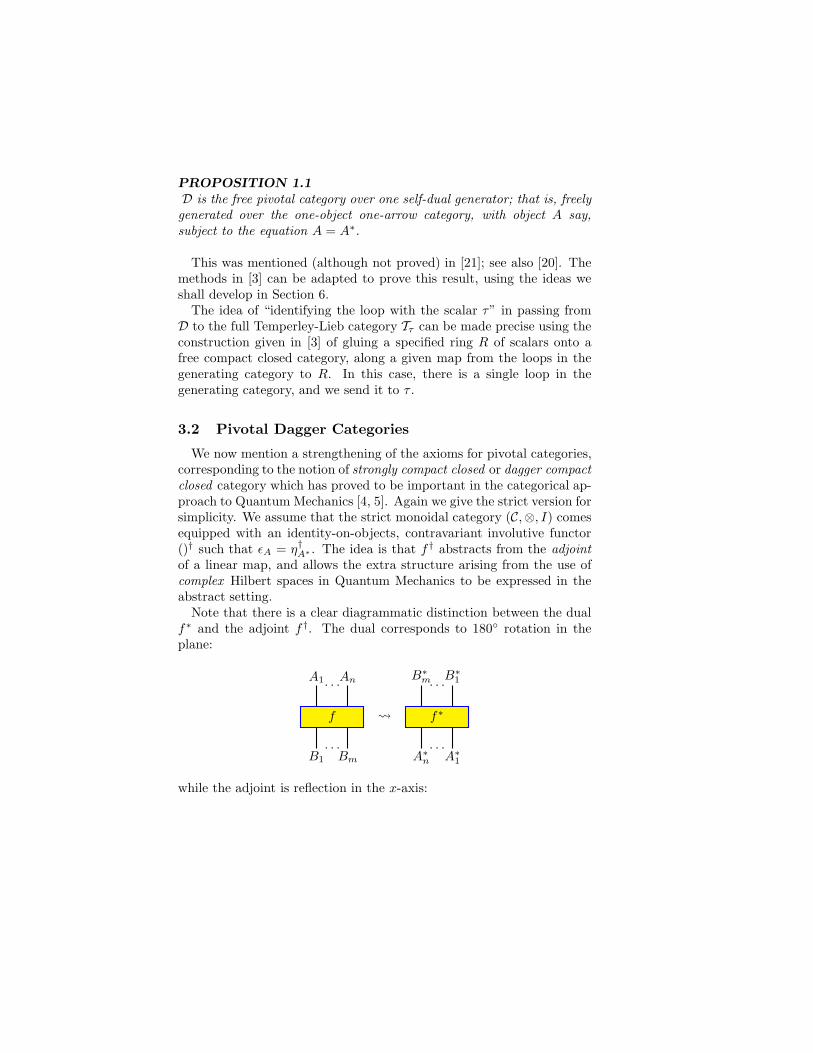
PROPOSITION 1.1

D is the free pivotal category over one self-dual generator; that is, freelygenerated over the one-object one-arrow category, with object A say,subject to the equation A = A∗.

This was mentioned (although not proved) in [21]; see also [20]. Themethods in [3] can be adapted to prove this result, using the ideas weshall develop in Section 6.

The idea of “identifying the loop with the scalar τ” in passing fromD to the full Temperley-Lieb category Tτ can be made precise using theconstruction given in [3] of gluing a specified ring R of scalars onto afree compact closed category, along a given map from the loops in thegenerating category to R. In this case, there is a single loop in thegenerating category, and we send it to τ .

3.2 Pivotal Dagger Categories

We now mention a strengthening of the axioms for pivotal categories,corresponding to the notion of strongly compact closed or dagger compactclosed category which has proved to be important in the categorical ap-proach to Quantum Mechanics [4, 5]. Again we give the strict version forsimplicity. We assume that the strict monoidal category (C,⊗, I) comesequipped with an identity-on-objects, contravariant involutive functor()† such that ǫA = η†A∗ . The idea is that f † abstracts from the adjointof a linear map, and allows the extra structure arising from the use ofcomplex Hilbert spaces in Quantum Mechanics to be expressed in theabstract setting.

Note that there is a clear diagrammatic distinction between the dualf∗ and the adjoint f †. The dual corresponds to 180◦ rotation in theplane:

f

· · ·A1 An

· · ·B1 Bm

f∗

· · ·B∗

m B∗1

· · ·A∗

n A∗1

while the adjoint is reflection in the x-axis:

f

· · ·A1 An

· · ·B1 Bm

f †

· · ·B1 Bn

· · ·A1 An

For example in D, if we consider the left and right wave morphisms Land R:

then we have

L∗ = L, L† = R, R∗ = R, R† = L.

Using the adjoint, we can define a covariant functor

f : A→ B

f∗ : A∗ → B∗f 7→ f∗†.

We have(f∗)∗ = f † = (f∗)

∗.

In terms of complex matrices, f∗ is transpose, while f∗ is complex con-jugation. Diagrammatically, f∗ is “reflection in the y-axis”.

f f∗ f † f∗

We have the following refinement of Proposition 1.1, by similar meth-ods to those used for free strongly compact closed categories in [3].

PROPOSITION 1.2

D is the free pivotal dagger category over one self-dual generator.

4 Factorization and Idempotents

We now consider some structural properties of the category D whichwe have not found elsewhere in the literature.4

We begin with a pleasingly simple diagrammatic characterization ofmonics and epics in D.

PROPOSITION 1.3

An arrow in D is monic iff it has no cups; it is epic iff it has no caps.

Proof Suppose that f : n → m has no cups. Thus all dots in n areconnected by through lines to dots in m. Now consider a compositionf ◦g. No loops can be formed by this composition; hence we can recoverg from f ◦ g by erasing the caps of f . Moreover, the number of loops inf ◦ g will simply be the sum of the loops in f and g, so we can recoverthe loops of g by subtracting the loops of f from the composition. Itfollows that

f ◦ g = f ◦ h =⇒ g = h,

i.e. that f is monic, as required.For the converse, suppose that f has a cup, which we can assume

to be connecting dots i and i + 1 in the top row. (Note that if i < jare connected by a cup, then by planarity, every k with i < k < jmust also be connected in a cup to some l with i < l < j.) Thenf ◦ δ · 1 = f ◦ (1 ⊗ Ui ⊗ 1), so f is not monic. Diagrammatically, thissays that we can either form a loop using the cup of f , or simply add aloop which is attached to an identity morphism.

The characterization of epics is entirely similar. �

This immediately yields an “image factorization” structure for D.

PROPOSITION 1.4

Every arrow in D has an epi-mono factorization.

Proof Given an arrow f : n→ m, suppose it has p cups and q caps.Then we obtain arrows e : n → (m − 2q) by erasing the caps, andm : (n−2p)→m by erasing the cups. By Proposition 1.3, e is epic and

4The idea of considering these properties arose from a discussion with Louis Kauff-man, who showed the author a direct diagrammatic characterization of idempotentsin D, which has subsequently appeared in [32].

m monic. Moreover, the number of dots in the top and bottom rowsconnected by through lines must be the same. Hence

(m− 2q) = k = (n− 2p),

and we can compose e and m to recover f . Note that by planarity, oncewe have assigned cups and caps, there is no choice about the correspon-dence between top and bottom row dots by through lines.

This factorization is “essentially” unique. However, we are free tosplit the l loops of f between e and m in any way we wish, so there is adistinct factorization δa ·m ◦ δb · e for all a, b ∈ N with a+ b = l. �

We illustrate the epi-mono factorization for the left wave:

=

We recall that an idempotent in a category is an arrow i : A → Asuch that i2 = i. We say that an idempotent i splits if there are arrowsr : A→ B and s : B → A such that

i = s ◦ r, r ◦ s = 1B.

PROPOSITION 1.5

All idempotents split in D.

Proof Let i : n → n be an idempotent in D. By Proposition 1.4,i = m ◦ e, where e : n→ k is epic and m : k→ n is monic. Now

m ◦ e ◦m ◦ e = m ◦ e.

Since m is monic, this implies that e ◦m ◦ e = e = 1 ◦ e. Since e is epic,this implies that e ◦m = 1. �

5 Categorical Quantum Mechanics

We now relate our discussion to the Abramsky-Coecke programme ofCategorical Quantum Mechanics.

This approach is very different to previous work on the Computer Sci-ence side of this interdisciplinary area, which has focussed on quantumalgorithms and complexity. The focus has rather been on developinghigh-level methods for Quantum Information and Computation (QIC)—languages, logics, calculi, type systems etc.—analogous to those whichhave proved so essential in classical computing [2]. This has led to noth-ing less than a recasting of the foundations of Quantum Mechanics itself,in the more abstract language of category theory. The key contributionis the paper with Coecke [4], in which we develop an axiomatic presen-tation of quantum mechanics in the general setting of strongly compactclosed categories, which is adequate for all the needs of QIC.

Specifically, we show that we can recover the key quantum mechan-ical notions of inner-product, unitarity, full and partial trace, Hilbert-Schmidt inner-product and map-state duality, projection, positivity, mea-surement, and Born rule (which provides the quantum probabilities), ax-iomatically at this high level of abstraction and generality. Moreover,we can derive the correctness of protocols such as quantum teleporta-tion, entanglement swapping and logic-gate teleportation [10, 24, 45] ina transparent and very conceptual fashion. Also, while at this level ofabstraction there is no underlying field of complex numbers, there is stillan intrinsic notion of ‘scalar’, and we can still make sense of dual vs. ad-joint [4, 5], and global phase and elimination thereof [15]. Peter Selingerrecovered mixed state, complete positivity and Jamiolkowski map-stateduality [42]. Recently, in collaboration with Dusko Pavlovic and Eric Pa-quette, decoherence, generalized measurements and Naimark’s theoremhave been recovered [17, 16].

Moreover, this formalism has two important additional features. Firstly,it goes beyond the standard Hilbert-space formalism, in that it is able tocapture classical as well as quantum information flows, and the interac-tion between them, within the formalism. For example, we can capturethe idea that the result of a measurement is used to determine a furtherstage of quantum evolution, as e.g. in the teleportation protocol [10],where a unitary correction must be performed after a measurement; oralso in measurement-based quantum computation [39, 40]. Secondly,this categorical axiomatics can be presented in terms of a diagrammaticcalculus which is extremely intuitive, and potentially can replace low-level computation with matrices by much more conceptual — and au-tomatable — reasoning. Moreover, this diagrammatic calculus can beseen as a proof system for a logic, leading to a radically new perspectiveon what the right logical formulation for Quantum Mechanics should

be. This latter topic is initiated in [6], and developed further in theforthcoming thesis of Ross Duncan.

5.1 Outline of the approach

We now give some further details of the approach. The general settingis that of strongly (or dagger) compact closed categories, which are thesymmetric version of the pivotal dagger categories we encountered inSection 3. Thus, in addition to the structure mentioned there, we havea symmetry natural isomorphism

σA,B : A⊗B ≃ B ⊗A.

See [5] for an extended discussion. An important feature of the Abramsky-Coecke approach is the use of an intuitive graphical calculus, which isessentially the diagrammatic formalism we have seen in the Temperley-Lieb setting, extended with more general basic types and arrows. Thekey point is that this formalism admits a very direct physical interpre-tation in Quantum Mechanics.

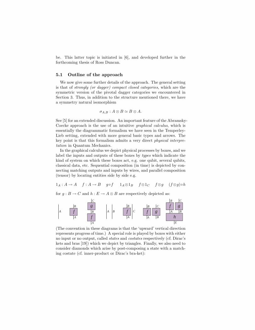
In the graphical calculus we depict physical processes by boxes, and welabel the inputs and outputs of these boxes by types which indicate thekind of system on which these boxes act, e.g. one qubit, several qubits,classical data, etc. Sequential composition (in time) is depicted by con-necting matching outputs and inputs by wires, and parallel composition(tensor) by locating entities side by side e.g.

1A : A→ A f : A→ B g◦f 1A⊗1B f⊗1C f⊗g (f⊗g)◦h

for g : B → C and h : E → A⊗B are respectively depicted as:

fB

A

gC

fB

B

gfB

A

C

A

fB

A

E

hA

C

A B fB

B

gC

A

(The convention in these diagrams is that the ‘upward’ vertical directionrepresents progress of time.) A special role is played by boxes with eitherno input or no output, called states and costates respectively (cf. Dirac’skets and bras [19]) which we depict by triangles. Finally, we also need toconsider diamonds which arise by post-composing a state with a match-ing costate (cf. inner-product or Dirac’s bra-ket):

ψA

A

πψ

Aπ

π ψo

=

that is, algebraically,

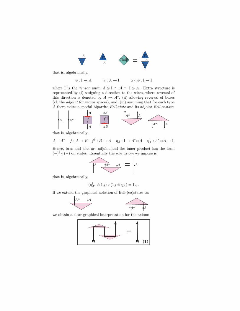
ψ : I→ A π : A→ I π ◦ ψ : I→ I

where I is the tensor unit : A ⊗ I ≃ A ≃ I ⊗ A. Extra structure isrepresented by (i) assigning a direction to the wires, where reversal ofthis direction is denoted by A 7→ A∗, (ii) allowing reversal of boxes(cf. the adjoint for vector spaces), and, (iii) assuming that for each typeA there exists a special bipartite Bell-state and its adjoint Bell-costate:

fA A* fA

A

B

BA

A

A*

A*

†

that is, algebraically,

A A∗ f : A→ B f † : B → A ηA : I→ A∗⊗A η†A : A∗⊗A→ I.

Hence, bras and kets are adjoint and the inner product has the form(−)† ◦ (−) on states. Essentially the sole axiom we impose is:

A AA* = A

that is, algebraically,

(η†A∗ ⊗ 1A) ◦ (1A ⊗ ηA) = 1A .

If we extend the graphical notation of Bell-(co)states to:

A

A

A*

A*

we obtain a clear graphical interpretation for the axiom:

=(1)

which now tells us that we are allowed to yank the black line straight :

=This equation and its diagrammatic counterpart should of course becompared to equation (2), and equation (1) and its accompanying di-agram, in Section 3— they are one and the same, subject to minordifferences in diagrammatic conventions.

This intuitive graphical calculus is an important benefit of the cate-gorical axiomatics. Other advantages can be found in [4, 2].

5.2 Quantum non-logic vs. quantum hyper-logic

The term quantum logic is usually understood in connection with the1936 Birkhoff-von Neumann proposal [11, 41] to consider the (closed)linear subspaces of a Hilbert space ordered by inclusion as the formal ex-pression of the logical distinction between quantum and classical physics.While in classical logic we have deduction, the linear subspaces of aHilbert space form a non-distributive lattice and hence there is no ob-vious notion of implication or deduction. Quantum logic was thereforealways seen as logically very weak, or even as a non-logic. In addi-tion, it has never given a satisfactory account of compound systems andentanglement.

On the other hand, compact closed logic in a sense goes beyond or-dinary logic in the principles it admits. Indeed, while in ordinary cate-gorical logic “logical deduction” implies that morphisms internalize aselements (which above we referred to above as states) i.e.

Bf- C

≃←→ I

⌈f⌉- B⇒C

(where I is the tensor unit), in compact closed logic they internalize bothas states and as costates, i.e.

A⊗B∗ ⌊f⌋- I

≃←→ A

f- B

≃←→ I

⌈f⌉- A∗⊗B

where we introduce the following notation:

pfq = (1A∗ ⊗ f) ◦ ηA : I → A∗⊗B xfy = ǫB ◦ (f ⊗ 1B∗) : A⊗B∗ → I.

It is exactly this dual internalization which allows the straightening ax-iom in picture (1) to be expressed. In the graphical calculus this iswitnessed by the fact that we can define both a state and a costate

=: f =:

fff

(2)

for each operation f . Physically, costates form the (destructive parts of)projectors, i.e. branches of projective measurements.

5.2.1 Compositionality.

The semantics is obviously compositional, both with respect to se-quential composition of operations and parallel composition of typesand operations, allowing the description of systems to be built up fromsmaller components. But we also have something more specific in mind:a form of compositionality with direct applications to the analysis ofcompound entangled systems. Since we have:

=f

g

= f

g

f

g

=

f

g

we obtain:

f

g

=

f

g

(3)

i.e. composition of operations can be internalized in the behavior ofentangled states and costates. Note in particular the interesting phe-nomenon of “apparant reversal of the causal order” which is the sourceof many quite mystical interpretations of quantum teleportation in terms

of “traveling backward in time” — cf. [35]. Indeed, while on the left,physically, we first prepare the state labeled g and then apply the costatelabeled f , the global effect is as if we first applied f itself first, and onlythen g.

5.2.2 Derivation of quantum teleportation.

This is the most basic application of compositionality in action. Imme-diately from picture (1) we can read the quantum mechanical potentialfor teleportation:

Alice Bob

=ψ ψ

Alice Bob Alice Bob

= ψ

This is not quite the whole story, because of the non-deterministic natureof measurements. But it suffices to introduce a unitary correction. Usingpicture (3) the full description of teleportation becomes:

f

=

fi i

fi-1

fi-1 =

where the classical communication is now implicit in the fact that theindex i is both present in the costate (= measurement-branch) and thecorrection, and hence needs to be sent from Alice to Bob.

The classical communication can be made explicit as a fully fledgedpart of the formalism, using additional types : biproducts in [4], and“classical objects” in [17]. This allows entire protocols, including theinterplay between quantum and classical information which is often theirmost subtle ingredient, to be captured and reasoned about rigorously ina single formal framework.

5.3 Remarks

We close this Section with some remarks. We have seen that the cate-gorical and diagrammatic setting for Quantum Mechanics developed byAbramsky and Coecke is strikingly close to that in which the Temperley-Lieb category lives. The main difference is the free recourse to symmetryallowed in the Abramsky-Coecke setting (and in the main intended mod-els for that setting, namely finite-dimensional Hilbert spaces with linearor completely positive maps). However, it is interesting to note thatin the various protocols and constructions in Quantum Information andComputation which have been modelled in that setting to date [4], thesymmetry has not played an essential role. The example of teleportationgiven above serves as an example.

This raises some natural questions:

How much of QM/QIC lives in the plane?

More precisely:

• Which protocols make essential use of symmetry?

• How much computational or information-processing power doesthe non-symmetric calculus have?

• Does braiding have some computational significance? (Remember-ing that between pivotal and symmetric we have braided stronglycompact closed categories) [21].

6 Planar Geometry of Interaction and the Temperley-Lieb Algebra

We now address the issue of giving what, so far as I know, is the firstdirect—or “fully abstract”—description of the Temperley-Lieb category.Since the category T is directly and simply described as the free R-linearcategory generated by D, we focus on the direct description of D.

Previous descriptions:

• Algebraic, by generators and relations - whether “locally”, of theTemperley-Lieb algebrasAn(τ), as in Jones’ presentation, or “glob-ally”, by a description of D as the free pivotal category, as inProposition 1.1.

• Kauffman’s topological description: diagrams “up to planar iso-topy”.

In fact, it is well known (see e.g. [33]) that the diagrams are completelycharacterized by how the dots are joined up — i.e. by discrete relationson finite sets. This leaves us with the problem of how to capture

1. Planarity

2. The multiplication of diagrams — i.e. composition in D

purely in terms of the data given by these relations.The answers to these questions exhibit the connections that exist be-

tween the Temperley-Lieb category and what is commonly known asthe “Geometry of Interaction”. This is a dynamical/geometrical inter-pretation of proofs and Cut Elimination initiated by Girard [23] as anoff-shoot of Linear Logic [22]. The general setting for these notions isnow known to be that of traced monoidal and compact closed categories— in particular, in the free construction of compact closed categoriesover traced monoidal categories [1, 7]. In fact, this general constructionwas first clearly described in [27], where one of the leading motivationswas the knot-theoretic context.

Our results in this Section establish a two-way connection. In onedirection, we shall use ideas from Geometry of Interaction to answerQuestion 2 above: that is, to define path composition (including the for-mation of loops) purely in terms of the discrete relations tabulating howthe dots are joined up. In the other direction, our answer to Question 1will allow us to consider a natural planar variant of the Geometry ofInteraction.

6.1 Some preliminary notions

6.1.1 Partial Orders

We use the notation P = (|P |,≤P ) for partial orders. Thus |P | isthe underlying set, and ≤P is the order relation (reflexive, transitiveand antisymmetric) on this set. An order relation is linear if for allx, y ∈ |P |, x ≤P y or y ≤P x.

Given a natural number n, we define [n] := {1 < · · · < n}, the linearorder of length n. We define several constructions on partial orders.Given partial orders P , Q, we define:

• The disjoint sum P ⊕ Q, where |P ⊕ Q| = |P | + |Q|, the disjointunion of |P | and |Q|, and

x ≤P⊕Q y ⇐⇒ (x ≤P y) ∨ (x ≤Q y).

• The concatenation P � Q, where |P � Q| = |P | + |Q|, with thefollowing order:

x ≤P�Q y ⇐⇒ (x ≤P y) ∨ (x ≤Q y) ∨ (x ∈ P ∧ y ∈ Q).

• P op = (|P |,≥P ).

Given elements x, y of a partial order P , we define:

x ↑ y ⇔ (x ≤P y) ∨ (y ≤P x)

x # y ⇔ ¬(x ↑ y).

6.1.2 Relations

A relation on a set X is a subset of the cartesian product: R ⊆ X×X .Since relations are sets, they are closed under unions and intersections.We shall also use the following operations of relation algebra:

Identity relation: 1X := {(x, x) | x ∈ X}

Relation composition: R;S := {(x, z) | ∃y. (x, y) ∈ R ∧ (y, z) ∈ S}

Relational converse: Rc := {(y, x) | (x, y) ∈ R}

Transitive closure: R+ :=⋃

k≥1Rk

Reflexive transitive closure: R∗ :=⋃

k≥0Rk

Here Rk is defined inductively: R0 := 1X , R1 := R, Rk+1 := R;Rk. Arelation R is single-valued or a partial function if Rc;R ⊆ 1X . It is totalif R;Rc ⊇ 1X . A function f : X → X is a single-valued, total relation.

These notions extend naturally to relations R ⊆ X × Y .

6.1.3 Involutions

A fixed-point free involution on a set X is a function f : X → X suchthat

f2 = 1X , f ∩ 1X = ∅.

Thus for such a function f(x) = y ⇔ x = f(y) and f(x) 6= x. We writeInv(X) for the set of fixed-point free involutions on a set X . Note thatInv(X) is not closed under function composition; nor does it containthe identity function. We must look elsewhere for suitable notions ofcomposition and identity.

An involution is equivalently described as a parition of X into 2-element subsets:

X =⋃

E, where E = {{x, y} | f(x) = y}. (3)

This defines an undirected graph Gf = (X,E). Clearly Gf is 1-regular[18]: each vertex has exactly one incident edge. Conversely, every graphG = (X,E) with this property determines a unique f ∈ Inv(X) withGf = G. Note that a finite set can only carry such a structure of itscardinality is even.

6.2 Formalizing diagrams

From our previous discussion, it is fairly clear how we will proceed toformalize morphisms n→m in D. Given n,m ∈ N, we define N(n,m) =[n]⊕ [m]. We visualize this partial order as

· · ·

· · · · · ·

1 2 n

1′ 2′ m′

We use the notation i′ to distinguish the elements of [m] in this disjointunion from those of [n], which are unprimed. Note that the order onN(n,m) has an immediate spatial interpretation in the diagrammaticrepresentation: i < j just in case i lies to the left of j on either the topor bottom line of dots, corresponding to [n] and [m] respectively.

A diagram connecting up dots pairwise will be formalized as a mapf ∈ Inv(|N(n,m)|). Such a map can be visualized by drawing undirectedarcs between the pairs of nodes i, j such that f(i) = j.

6.2.1 Example

The map f ∈ Inv(|N(4, 2)|) such that

f : 1↔ 2′, 2↔ 4, 3↔ 1′

is depicted thus:1 2 3 4

1′ 2′

Our task is now is characterize those involutions which are planar.The key idea is that this can be done using just the order relations wehave introduced.

6.3 Characterizing Planarity

A map f ∈ Inv(|N(n,m)|) will be called planar if it satisfies the fol-lowing two conditions, for all i, j ∈ N(n,m):

(PL1) i < j < f(i) =⇒ i < f(j) < f(i)

(PL2) f(i) # i < j # f(j) =⇒ f(i) < f(j).

It is instructive to see which possibilities are excluded by these condi-tions.

6.3.1 First condition

(PL1) i < j < f(i) =⇒ i < f(j) < f(i)

(PL1) rules out

· · ·

· · ·

i j f(i)

f(j)

where f(j) # f(i), and also

i j f(i) f(j)

where f(i) < f(j).

6.3.2 Second condition

(PL2) f(i) # i < j # f(j) =⇒ f(i) < f(j).

Similarly, (PL2) rules out

· · · · · ·

· · ·

i j

f(j) f(i)

We write P(n,m) for the set of planar maps in Inv(|N(n,m)|).

PROPOSITION 1.6

1. Every planar diagram satisfies the two conditions.

2. Every involution satisfying the two conditions can be drawn as aplanar diagram.

Rather than proving this directly, it is simpler, and also instructive, toreduce it to a special case. We consider arrows in D of the special formI → n. Such arrows consist only of caps. They correspond to points, orstates in the terminology of Section 5.

Since the top row of dots is empty, in this case we have a linear order,and the premise of condition (PL2) can never arise. Hence planarityfor such arrows is just the simple condition (PL1) — which can be seento be equivalent to saying that, if we write a left parenthesis for eachleft end of a cap, and a right parenthesis for each right end, we get awell-formed string of parentheses. Thus

corresponds to()(()).

(Of course, exactly similar comments apply to arrows of the form n→ I,i.e. costates.) It is also clear5 that Proposition 1.6 holds for such arrows.

Now we recall that quite generally, in any pivotal category we havethe Hom-Tensor adjunction

A⊗B∗ ⌊f⌋- I

≃←→ A

f- B

≃←→ I

⌈f⌉- A∗⊗B

pfq = (1A∗ ⊗ f) ◦ ηA : I → A∗⊗B xfy = ǫB ◦ (f ⊗ 1B∗) : A⊗B∗ → I.

We call pfq the name of f , and xfy the coname. The inverse to themap f 7→ pfq is defined by

g : I → A∗ ⊗B 7→ (ǫA ⊗ 1B) ◦ (1A ⊗ g) : A→ B.

For example, we compute the name of the left wave:

=

Applying the inverse transformation:

=

Note also that the unit is the name of the identity: ηn = p1nq, andsimilarly ǫn = x1ny.

Thus we see that diagrammatically, the process of forming the nameof an arrow involves reversing the left-right order of the top row of dotsby rotating them concentrically, and sliding them down to lie parallelwith, and to the left of, the bottom row. In this process, cups are turned

5With an implicit appeal to the Jordan Curve Theorem!

into caps, while through lines are stretched out and turned to also formcaps.

This transposition of the top row of dots can be described order-theoretically, as replacing the partial order [n]⊕ [m] by the linear order[n]op

� [m]. Note that the underlying sets of these two partial orders arethe same: |[n] ⊕ [m]| = |[n]op

� [m]|. Thus pfq is essentially the samefunction as f .

PROPOSITION 1.7

For f ∈ Inv(|N(n,m)|), the following are equivalent:

1. f satisfies (PL1) and (PL2) with respect to [n]⊕ [m].

2. f satisfies (PL1) with respect to [n]op� [m].

Proof Firstly, assume (2), and suppose f(i) # i < j # f(j). Ifi < j in the bottom row, then f(j) < i < j in [n]op

� [m], so by (PL1),f(j) < f(i) < j, i.e. f(i) < f(j) in [n]⊕ [m], as required. Now supposei < j in the top row. Then j < i < f(j) in [n]op

� [m], so by (PL1),j < f(i) < f(j), and in particular f(i) < f(j).

Now assume (1), and suppose that i < j < f(i) in [n]op� [m]. The

interesting case is where i is in the top row and f(i) in the bottomrow. We need to do some case analysis. Suppose firstly that j is in thetop row. If f(j) is in the bottom row, then f(j) # j < i # f(i) in[n] ⊕ [m], and we can apply (PL2) to conclude that f(j) < f(i), andhence i < f(j) < f(i) in [n]op

� [m]. If f(j) is in the top row, we musthave f(j) < i by (PL1) for [n] ⊕ [m], and hence i < f(j) < f(i) in[n]op

� [m].Now suppose that j is in the bottom row. If f(j) is in the bottom

row, we must have f(j) < f(i) by (PL1). If f(j) is in the top row, thenwe have f(j) # j < f(i) # i in [n]⊕ [m], so by (PL2) we have f(j) < i,and hence i < f(j) < f(i) in [n]op

� [m]. �

Since (PL1) characterizes planarity for pfq, it follows that (PL1) and(PL2) characterize planarity for f .

6.4 The Temperley-Lieb Category

Our aim is now to define a category TL, which will yield the desireddescription of the diagrammatic category D. The objects of TL are thenatural numbers. The homset TL(n,m) is defined to be the cartesianproduct N×P(n,m). Thus a morphism n→m in TL consists of a pair

(k, f), where k is a natural number, and f ∈ P(n,m) is a planar map inInv(|N(n,m)|). The idea is that k is a counter for the number of loops,so such an arrow can be written δk · f in the notation used previously.

It remains to define the composition and identities in this category.Clearly (even leaving aside the natural number components of mor-phisms) composition cannot be defined as ordinary function composi-tion. This does not even make sense — the codomain of an involutionf ∈ P(n,m) does not match the domain of an involution g ∈ P(m, p) —let alone yield a function with the necessary properties to be a morphismin the category.

6.4.1 Composition: The “Execution Formula”

Consider a map f : [n]+[m] −→ [n]+[m]. Each input lies in either [n]or [m] (exclusive or), and similarly for the corresponding output. Thisleads to a decomposition of f into four disjoint partial maps :

fn,n : [n] −→ [n] fn,m : [n] −→ [m]

fm,n : [m] −→ [n] fm,m : [m] −→ [m]

so that f can be recovered as the disjoint union of these four maps. Iff is an involution, then these maps will be partial involutions.

Note that these components have a natural diagrammatic reading:fn,n describes the cups of f , fm,m the caps, and fn,m = f c

m,n the throughlines.

Now suppose we have maps f : [n]+[m]→ [n]+[m] and g : [m]+[p]→[m] + [p]. We write the decompositions of f and g as above in matrixform:

f =

fn,n fn,m

fm,n fm,m

g =

gm,m gm,p

gp,m gp,p

We can view these maps as binary relations on [n] + [m] and [m] + [p]respectively, and use relational algebra (union R ∪ S, relational compo-sition R;S and reflexive transitive closure R∗) to define a new relationθ on [n] + [p]. If we write

θ =

θn,n θn,p

θp,n θp,p

so that θ is the disjoint union of these four components, then we candefine it component-wise as follows:

θn,n = fn,n ∪ fn,m; gm,m; (fm,m; gm,m)∗; fm,n

θn,p = fn,m; (gm,m; fm,m)∗; gm,p

θp,n = gp,m; (fm,m; gm,m)∗; fm,n

θp,p = gp,p ∪ gp,m; fm,m; (gm,m; fm,m)∗; gm,p.

We can give clear intuitive readings for how these formulas express com-position of paths in diagrams in terms of relational algebra:

• The component θn,n describes the cups of the diagram resultingfrom the composition. These are the union of the cups of f (fn,n),together with paths that start from the top row with a throughline of f , given by fn,m, then go through an alternating odd-lengthsequence of cups of g (gm,m) and caps of f (fm,m), and finallyreturn to the top row by a through line of f (fm,n).

· · ·

• Similarly, θp,p describes the caps of the composition.

• θn,p = θcp,n describe the through lines. Thus θn,p describes paths

which start with a through line of f from n to m, continue withan alternating even-length (and possibly empty) sequence of cupsof g and caps of f , and finish with a through line of g from m top.

· · ·

All through lines from n to p must have this form.

This formula corresponds to the interpretation of Cut-Elimination in theGeometry of Interaction interpretation of proofs in Linear Logic (and byextension in related logics and type theories) [23]. A more abstract andgeneral perspective on how this construction arises can be given in thesetting of traced monoidal categories [27, 1].

PROPOSITION 1.8

If f and g are planar, so is θ.

We write θ = g ⊙ f ∈ P(n, p)

6.4.2 Cycles

Given f ∈ P(n,m), g ∈ P(m, p), we define χ(f, g) := fm,m; gm,m.Note that χ(f, g)c = (gm,m; fm,m), and

χ(f, g);χ(f, g)c ⊆ 1[m], χ(f, g)c;χ(f, g) ⊆ 1[m].

Thus χ(f, g) is a partial bijection. However, in general it is neither aninvolution, nor fixpoint-free. The cyclic elements of χ(f, g) are thoseelements of [m] which lie in the intersection

χ(f, g)+ ∩ 1[m].

· · ·

Thus if i is a cyclic element, there is a least k > 0 such that χ(f, g)k(i) =i. The corresponding cycle is

{i, χ(f, g)(i), . . . , χ(f, g)k−1(i)}.

Distinct cycles are disjoint. We write Z(f, g) for the number of distinctcycles of χ(f, g).

6.4.3 Composition and Identities

Finally, we define the composition of morphisms in TL. Given (s, f) :n→m and (t, g) : m→ p:

(t, g) ◦ (s, f) = (s+ t+ Z(f, g), g ⊙ f).

The identity morphism idn : n→ n is defined to be the pair (0, τn,n),where τn,n is the twist map on [n] + [n]; i.e. the involution i ↔ i′.Diagrammatically, this is just

· · ·

· · ·

1 2 n

1′ 2′ n′

Note that this is not the identity map on [n] + [n] — indeed it is (nec-essarily) fixpoint free!

PROPOSITION 1.9

TL with composition and identities as defined above is a category.

6.4.4 TL as a pivotal category

The monoidal structure of TL is straightforward. If (k, f) : n → mand (l, g) : p → q, then (k + l, f + g) : n + p → m + q, where f + g ∈P(n+ p,m+ q) is the evident disjoint union of the involutions f and g.

The unit ηn : I → n + n is given by

i↔ i′ (1 ≤ i ≤ n),

and similarly for the counit. Note that identities, units and counits areall essentially the same maps, but with distinct types, which partitiontheir arguments between inputs and outputs differently.

We describe the dual, adjoint and conjugate of an arrow (k, f) : n→

m. Let τn,m : [n] + [m]∼=−→ [m] + [n] be the symmetry isomorphism of

the disjoint union, and

ρn : [n]∼=−→ [n] :: i 7→ n− i+ 1

be the order-reversal isomorphism. Note that

τ−1n,m = τm,n, ρ−1

n = ρn, τn,m ◦ (ρn + ρm) = (ρm + ρn) ◦ τn,m.

Then we have (k, f)• = (k, f•), where:

f † = τn.m ◦ f ◦ τ−1n,m

f∗ = (ρn + ρm) ◦ f ◦ (ρn + ρm)−1

f∗ = (f †)∗.

6.4.5 The Main Result

THEOREM 1.1

TL is isomorphic as a strict, pivotal dagger category to D.

As an immediate Corollary of this result and Proposition 1.2, we have:

THEOREM 1.2

TL is the free strict, pivotal dagger category on one self-dual generator.

This is in the same spirit as the characterizations of free compact anddagger compact categories in [34, 3].

These results can easily be extended to descriptions of the free pivotaldagger category over an arbitrary generating category, leading to ori-ented Temperley-Lieb algebras with primitive (physical) operations. Werefer to [3] for a more detailed presentation (in the symmetric case).

7 Planar λ-Calculus

Our aim in this section is to show how a restricted form of λ-calculuscan be interpreted in the Temperley-Lieb category, and how β-reductionof λ-terms, which is an important foundational paradigm for compu-tation, is then reflected diagrammatically as geometric simplification,i.e. “yanking lines straight”. We can give only a brief indication of whatis in fact a rich topic in its own right. See [6, 7, 31] for discussions ofrelated matters.

7.1 The λ-Calculus

We begin with a (very) brief review of the λ-calculus [14, 9], whichis an important foundational paradigm in Logic and Computation, andin particular forms the basis for all modern functional programminglanguages.

The syntax of the λ-calculus is beguilingly simple. Given a set ofvariables x, y, z, . . . we define the set of terms as follows:

t ::= x | tu︸︷︷︸

application

| λx. t︸︷︷︸

abstraction

Notational Convention: We write

t1t2 · · · tk ≡ (· · · (t1t2) · · ·)tk.

Some examples of terms:

λx. x identity function

λf. λx. fx application

λf. λx. f(fx) double application

λf. λg. λx. g(f(x)) composition g ◦ f

The basic equation governing this calculus is β-conversion:

(λx. t)u = t[u/x]

E.g. (assuming some arithmetic operations are given)

(λf. λx. f(fx))(λx. x + 1)0 = (0 + 1) + 1 = 2.

By orienting this equation, we get a ‘dynamics’ — β-reduction

(λx. t)u→ t[u/x]

Despite its sparse syntax, λ-calculus is very expressive—it is in fact auniversal model of computation, equivalent to Turing machines.

7.2 Types

One important way of constraining the λ-calculus is to introduceTypes.

Types are there to stop you doing (bad) things

Types are in fact one of the most fruitful positive ideas in ComputerScience!

We shall introduce a (highly restrictive) type system, such that thetypable terms can be interpreted in the Temperley-Lieb category (infact, in any pivotal category).

Firstly, assuming some set of basic types B, we define a syntax ofgeneral types:

T ::= B | T → T.

Intuitively, T → U represents the type of functions which take inputs oftype T to outputs of type U .Notational Convention: We write

T1 → T2 → · · ·Tk → Tk+1 ≡ T1 → (T2 → · · · (Tk → Tk+1) · · ·).

Examples:

A→ A→ A first-order function type

(A→ A)→ A second-order function type

We now introduce a formal system for deriving typing judgements, ofthe form:

x1 : T1, . . . xk : Tk ⊢ t : T.

Such a judgement asserts that the term t has type T under the assump-tion (or: in the context) that the variable x1 has type T1, . . . , xk hastype Tk. All the variables xi appearing in the context must be distinct— and in our setting, the order in which the variables appear in the listis significant.There is one basic form of axiom, for typing variables:

Variablex : T ⊢ x : T

and two inference rules, for typing abstractions and applications respec-tively:

Function

Γ, x : U ⊢ t : T

Γ ⊢ λx. t : U → TΓ ⊢ t : U → T ∆ ⊢ u : U

Γ,∆ ⊢ tu : T

Note that Γ,∆ represents the concatenation of the lists Γ, ∆. This im-plies that the variables appearing in Γ and ∆ are distinct—an importantlinearity constraint in the sense of Linear Logic [22].

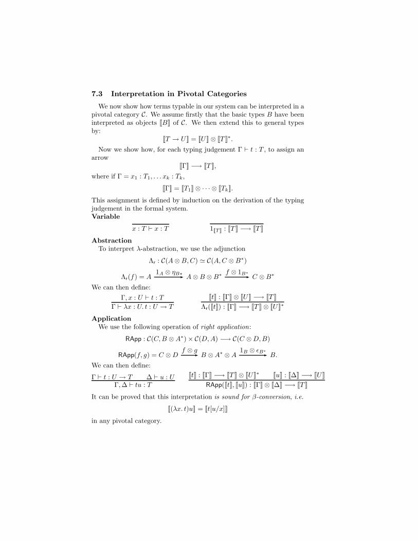
7.3 Interpretation in Pivotal Categories

We now show how terms typable in our system can be interpreted in apivotal category C. We assume firstly that the basic types B have beeninterpreted as objects JBK of C. We then extend this to general typesby:

JT → UK = JUK⊗ JT K∗.

Now we show how, for each typing judgement Γ ⊢ t : T , to assign anarrow

JΓK −→ JT K,

where if Γ = x1 : T1, . . . xk : Tk,

JΓK = JT1K⊗ · · · ⊗ JTkK.

This assignment is defined by induction on the derivation of the typingjudgement in the formal system.Variable

x : T ⊢ x : T 1JT K : JT K −→ JT K

AbstractionTo interpret λ-abstraction, we use the adjunction

Λr : C(A⊗B,C) ≃ C(A,C ⊗B∗)

Λr(f) = A1A ⊗ ηB∗

- A⊗B ⊗B∗ f ⊗ 1B∗

- C ⊗B∗

We can then define:

Γ, x : U ⊢ t : T

Γ ⊢ λx : U. t : U → T

JtK : JΓK⊗ JUK −→ JT K

Λr(JtK) : JΓK −→ JT K⊗ JUK∗

ApplicationWe use the following operation of right application:

RApp : C(C,B ⊗A∗)× C(D,A) −→ C(C ⊗D,B)

RApp(f, g) = C ⊗Df ⊗ g

- B ⊗A∗ ⊗A1B ⊗ ǫB∗

- B.

We can then define:

Γ ⊢ t : U → T ∆ ⊢ u : UΓ,∆ ⊢ tu : T

JtK : JΓK −→ JT K⊗ JUK∗ JuK : J∆K −→ JUK

RApp(JtK, JuK) : JΓK⊗ J∆K −→ JT K

It can be proved that this interpretation is sound for β-conversion, i.e.

J(λx. t)uK = Jt[u/x]K

in any pivotal category.

7.4 An Example

We now discuss an example to show how all this works diagrammati-cally in TL. We shall consider the bracketing combinator

B ≡ λx.λy.λz. x(yz).

This is characterized by the equation

Babc = a(bc).

Firstly, we derive a typing judgement for this term:

x : B → C ⊢ x : B → C

y : A→ B ⊢ y : A→ B z : A ⊢ z : A

y : A→ B, z : A ⊢ yz : B

x : B → C, y : A→ B, z : A ⊢ x(yz) : C

x : B → C, y : A→ B ⊢ λz. x(yz) : A→ C

x : B → C ⊢ λy.λz. x(yz) : (A→ B)→ (A→ C)

⊢ λx.λy.λz. x(yz) : (B → C)→ (A→ B)→ (A→ C)

Now we take A = B = C = 1 in TL. The interpretation of the openterm

x : B → C, y : A→ B, z : A ⊢ x(yz) : C

is as follows:x+ x− y+ y− z+

o

Here x+ is the output of x, and x− the input, and similarly for y. Theoutput of the whole expression is o. When we abstract the variables, weobtain the following caps-only diagram:

x+x−y+y−z+o

Now we consider an application Babc:

x+x−y+y−z+o

a b c a b c

o

=

7.5 Discussion

The typed λ-calculus we have used here is in fact a fragment of theLambek calculus [36], a basic non-commutative logic and λ-calculus,which has found extensive applications in computational linguistics [13,38]. The Lambek calculus can be interpreted in any monoidal biclosedcategory, and has notions of left abstraction and application, as well asthe right-handed versions we have described here. Pivotal categorieshave stronger properties than monoidal biclosure; for example, dualityand adjoints allow the left- and right-handed versions of abstraction andapplication to be defined in terms of each other. Moreover, the dualitymeans that the corresponding logic has a classical format, with an invo-lutive negation. Thus there is much more to this topic than we have hadthe time to discuss here. We merely hope to have given an impression ofhow the geometric ideas expressed in the Temperley-Lieb category havenatural connections to a central topic in Logic and Computation.

8 Further Directions

We hope to have given an indication of the rich and suggestive con-nections which exist between ideas stemming from knot theory, topologyand mathematical physics, on the one hand, and logic and computationon the other, with the Temperley-Lieb category serving as an intuitiveand compelling meeting point. We hope that further investigation willuncover deeper links and interplays, leading to new insights in bothdirections.

We conclude with a few specific directions for future work:

• The symmetric case, where we drop the planarity constraint, is alsointeresting. The algebraic object corresponding to the Temperley-Lieb algebra in this case is the Brauer algebra [12], importantin the representation theory of the Orthogonal group (Schur-Weylduality). Indeed, there are now a family of various kinds of diagramalgebras: partition algebras, rook algebras etc., arising in quantumstatistical mechanics, and studied in Representation Theory [25].

• The categorical perspective suggests oriented versions of the Temperley-Lieb algebra and related structures, where we no longer have A =A∗. This is also natural from the point of view of QuantumMechanics, where this non-trivial duality on objects distinguishescomplex from real Hilbert spaces.

• We can ask how expressive planar Geometry of Interaction is; andwhat role may be played by braiding or other geometric informa-tion.

• Again, it would be interesting to understand the scope and limits ofplanar Quantum Mechanics and Quantum information processing.

References

[1] S. Abramsky. Retracing some paths in process algebra. In U. Mon-tanari and V. Sassone, editors, Proceedings of CONCUR ‘96, vol-ume 1119 of Springer Lecture Notes in Computer Science, pages1–17. Springer-Verlag, 1996.

[2] S. Abramsky. High-level methods for quantum computation andinformation. In Proceedings of the 19th Annual IEEE Symposiumon Logic in Computer Science, pages 410–414. IEEE ComputerScience Press, 2004.

[3] S. Abramsky. Abstract scalars, loops, and free traced and stronglycompact closed categories. In J. Fiadeiro, editor, Proceedings ofCALCO 2005, volume 3629 of Springer Lecture Notes in ComputerScience, pages 1–31. Springer-Verlag, 2005.

[4] S. Abramsky and B. Coecke. A categorical semantics of quantumprotocols. In Proceedings of the 19th Annual IEEE Symposiumon Logic in Computer Science, pages 415–425. IEEE ComputerScience Press. quant-ph/0402130, 2004.

[5] S. Abramsky and B. Coecke. Abstract physical traces. Theory andApplications of Categories, 14:111–124, 2005.

[6] S. Abramsky and R. W. Duncan. A categorical quantum logic.Mathematical Structures in Computer Science, 16:469–489, 2006.

[7] S. Abramsky, E. Haghverdi, and P. J. Scott. Geometry of interac-tion and linear combinatory algebras. Mathematical Structures inComputer Science, 12:625–665, 2002.

[8] S. Abramsky and R. Jagadeesan. New foundations for the geometryof interaction. Information and Computation, 111:53–119, 1994.

[9] H. P. Barendregt. The Lambda Calculus, volume 103 of Studies inLogic. North-Holland, 1984.

[10] C. H. Bennet, G. Brassard, C. Crepeau, R. Jozsa, A. Peres, andW. K. Wooters. Teleporting an unknown quantum state via dualclassical and Einstein-Podolsky-Rosen channels. Physical ReviewLetters, 70:1895–1899, 1993.

[11] G. Birkhoff and J. von Neumann. The logic of quantum mechanics.Annals of Mathematics, 37:823–843, 1936.

[12] R. Brauer. On algebras which are connected with the semisimplecontinuous groups. Ann. Math., 38:854–872, 1937.

[13] W. Buszkowski. Mathematical linguistics and proof theory. InJ. van Benthem and A. ter Meulen, editors, Handbook of Logic andLanguage, chapter 12, pages 683–736. Elsevier, 1997.

[14] A. Church. The Calculi of Lambda Conversion. Princeton Univer-sity Press, 1941.

[15] B. Coecke. De-linearizing linearity: projective quantum axiomat-ics from strong compact closure. Electronic Notes in TheoreticalComputer Science, 2006. To appear.

[16] B. Coecke and E. O. Paquette. Generalized measurements andNaimark’s theorem without sums. To appear in Fourth Workshopon Quantum Programming Languages, 2006.

[17] B. Coecke and D. Pavlovic. Quantum measurements without sums.In G. Chen, L. Kauffman, and S. Lamonaco, editors, Mathematicsof Quantum Computing and Technology. Taylor and Francis, 2006.To appear.

[18] J. Diestel. Graph Theory. Springer-Verlag, 1997.

[19] P. A. M. Dirac. The Principles of Quantum Mechanics (third edi-tion). Oxford University Press, 1947.

[20] K. Dosen and Z. Petric. Self-adjunctions and matrices. Journal ofPure and Applied Algebra, 184:7–39, 2003.

[21] P. Freyd and D. Yetter. Braided compact closed categories with ap-plications to low-dimensional topology. Advances in Mathematics,77:156–182, 1989.

[22] J.-Y. Girard. Linear Logic. Theoretical Computer Science, 50(1):1–102, 1987.

[23] J.-Y. Girard. Geometry of Interaction I: Interpretation of SystemF. In R. Ferro, editor, Logic Colloquium ’88, pages 221–260. North-Holland, 1989.

[24] D. Gottesman and I. L. Chuang. Quantum teleportation is a uni-versal computational primitive. Nature, 402:390–393, 1999.

[25] T. Halvorson and A. Ram. Partition algebras. European J. ofCombinatorics, 26(1):869–921, 2005.

[26] V. F. R. Jones. A polynomial invariant for links via von Neumannalgebras. Bulletin of the Amer. Math. Soc., 129:103–112, 1985.

[27] A. Joyal, R. Street, and D. Verity. Traced monoidal categories.Mathematical Proceedings of the Cambridge Philosophical Society,119:447–468, 1996.

[28] C. Kassel. Quantum Groups. Springer, 1995.

[29] L. H. Kauffman. An invariant of regular isotopy. Trans. Amer.Math. Soc., 318(2):417–471, 1990.

[30] L. H. Kauffman. Knots in Physics. World Scientific Press, 1994.

[31] L. H. Kauffman. Knot Logic. In L. H. Kauffman, editor, Knotsand Applications, pages 1–110. World Scientific Press, 1995.

[32] L. H. Kauffman. Biologic II. In N. Tongring and R. C. Penner,editors, Woods Hole Mathematics, pages 94–132. World ScientificPress, 2004.

[33] L. H. Kauffman. Knot diagrammatics. In W. W. Menasco andM. Thistlethwaite, editors, Handbook of Knot Theory. Elsevier,2005.

[34] G. M. Kelly and M. L. Laplaza. Coherence for compact closedcategories. Journal of Pure and Applied Algebra, 19:193–213, 1980.

[35] M. Laforest, R. Laflamme, and J. Baugh. Time-reversal formal-ism applied to maximal bipartite entanglement: Theoretical andexperimental exploration. quant-ph/0510048. Unpublished.

[36] J. Lambek. The mathematics of sentence structure. Amer. Math.Monthly, 65:154–170, 1958.

[37] R. Milner. Fully abstract models of typed lambda-calculus. Theo-retical Computer Science, 4:1–22, 1977.

[38] M. Moortgat. Categorial type logic. In J. van Benthem and A. terMeulen, editors, Handbook of Logic and Language, chapter 2, pages93–177. Elsevier, 1997.

[39] R. Raussendorf and H.-J. Briegel. A one-way quantum computer.Physical Review Letters, 86:5188, 2001.

[40] R. Raussendorf, D. Browne, and H.-J. Briegel. Measurement-based quantum computation on cluster states. Physical ReviewA, 68:022312, 2003.

[41] M. Redei. Why John von Neumann did not like the Hilbert spaceformalism of quantum mechanics (and what he liked instead).Studies in History and Philosophy of Modern Physics, 27:493–510,1997.

[42] P. Selinger. Dagger compact closed categories and completely posi-tive maps. Electronic Notes in Theoretical Computer Science, 2006.To appear.

[43] H. N. V. Temperley and E. H. Lieb. Relations between the ‘percola-tion’ and ‘coloring’ problem and other graph-theoretical problemsassociated with regular planar lattices: some exact results for the‘percolation’ problem. Proc. Roy. Soc. Lond. A, 322:251–280, 1971.

[44] E. Witten. Topological quantum field theory. Communications inMathematical Physics, 117:353—386, 1988.

[45] M. Zukowski, A. Zeilinger, M. A. Horne, and A. K. Ekert.‘Event-ready-detectors’ Bell experiment via entanglement swap-ping. Physical Review Letters, 71:4287–4290, 1993.

CRC PRESS

Boca Raton Ann Arbor London Tokyo