Temperature Trends at the Surface and in the Troposphere

Temperature Trends at the Surface and in the Troposphere

Konstantin Y. Vinnikov1, Norman C. Grody2, Alan Robock3, Ronald J. Stouffer4,

Philip D. Jones5, and Mitchell D. Goldberg2

1Department of Atmospheric and Oceanic Science, University of Maryland, College Park, MD, USA

2NOAA/NESDIS, Camp Springs, MD, USA 3Department of Environmental Sciences, Rutgers University, New Brunswick, NJ, USA 4Geophysical Fluid Dynamics Laboratory, NOAA, Princeton, NJ, USA 5Climate Research Unit, University of East Anglia, Norwich, UK

Submitted to Journal of Geophysical Research

June 2005 Corresponding author: Alan Robock Department of Environmental Sciences Rutgers University 14 College Farm Road New Brunswick, NJ 08901-8551 Phone: 732-932-9478 Fax: 732-932-8644 E-mail: [email protected]

2

Abstract

This paper incorporates the latest improvements in inter-satellite calibration, along with a

new statistical technique, to determine the diurnal and seasonal cycles and climatic trends of

1978-2004 tropospheric temperature using Microwave Sounding Unit measurements. We also

compare the latitudinal distribution of temperature trends from the surface and troposphere with

each other and with model simulations during the past 26 years. The observations at the surface

and troposphere are consistent with climate model simulations. At mid- and high latitudes in the

Northern Hemisphere, the zonally averaged temperature at the surface increased faster than in

the troposphere while at low latitudes of both hemispheres the temperature increased more

slowly at the surface than in the troposphere. The resulting global averaged tropospheric trend is

+0.20 K/10 yr, with a standard error of 0.05 K/10 yr, which compares very well with the trend

obtained from surface reports.

3

1. Introduction

The global temperature trend is difficult to measure since natural climate variability and

observation errors can have random trend-like warming and cooling for limited time intervals,

which can lead to errors and even mask the climatic trends. To reduce these errors and improve

the accuracy of the trend, one needs to improve the data accuracy and increase the record length.

Century-long surface air temperature records were used to detect a global climate trend prior to

the existence of satellite measurements. More recently, the overlapping time series of satellite

measurements from the Microwave Sounding Unit (MSU) have been used to detect the

tropospheric temperature trend over the past 25 years [Mears et al., 2003; Vinnikov and Grody,

2003; Christy and Norris, 2004]. This study uses a more accurate inter-satellite calibration

technique [Grody et al., 2004] together with diurnal cycle corrections [Vinnikov and Grody,

2003; Vinnikov et al, 2004] to improve the trend analysis. In addition to obtaining the global

trend, we compare the MSU latitudinal distribution of trend with those determined from surface

air temperature measurements and climate model simulations.

Microwave radiometers such as the MSU measure the temperature emanating from

different layers of the Earth’s atmosphere by detecting the thermally emitted radiation at

different frequencies within the 50-60 GHz portion of the oxygen band. Calibration of the

radiometers is obtained by viewing cold space and an onboard warm target of known

temperature at the beginning and end of every scan cycle. Between calibration periods, the MSU

views the Earth and measures the upwelling thermal radiation, or brightness temperature, at four

frequencies within the oxygen band. The nadir viewing measurements at 53.74 GHz (denoted

channel 2) mainly respond to temperature variations in the middle troposphere, so this channel is

used to monitor changes in tropospheric temperature. Besides responding best to tropospheric

4

temperature, the near nadir measurements eliminate the need for angular (i.e., local zenith angle)

adjustments of the measurements as the MSU scans from nadir, or as the satellite height changes

due to orbital drift.

In addition to the tropospheric contribution, approximately 10% of the radiation

measured by MSU channel 2 results from changes in surface temperature and another 10% from

the atmosphere above 180 hPa. It is important to recognize, however, that unlike the changes in

temperature, surface emissivity only results in a 1% variation because of the compensating

surface emitted and downwelling reflected radiation [Grody et al., 2004]. Therefore, the change

in the globally averaged measurements due to temporal variations in emissivity (e.g., due to

changes in sea ice, snow cover, or soil wetness) is negligibly small. Of greater importance is the

diurnal variation in surface temperature due to orbital drift and the different satellite observing

times. Such diurnal variations must be accounted for when constructing a time series using the

26 years of satellite measurements.

We also recognize that the MSU channel 2 brightness temperature trend may be

underestimated compared to in situ tropospheric temperature warming because of stratospheric

cooling [Fu et al., 2004; Fu and Johanson, 2005], but this subject needs more accurate

evaluation using correctly calibrated data for all four MSU channels. It is important to note,

however, that the climate model simulations of MSU channel 2 used here include both the

surface and stratospheric contributions, so that our comparisons between modeled and observed

channel 2 brightness temperatures are completely valid. Stated differently, rather than adjust the

channel 2 measurements we have chosen to include the surface and stratospheric contributions in

the MSU climate model simulations, which are then compared directly with the satellite

measurements.

5

Of major importance is the latest improvement of inter-satellite calibration [Grody et al.,

2004], which we apply to the MSU channel 2 measurements to enable a more accurate global

temperature trend, in addition to its latitudinal distribution, over the period 1978-2004. Until

now, empirical procedures have been used to inter-calibrate the MSU observations. Previous

researchers [Christy et al., 2000; Mears et al., 2003] assumed that the error in the MSU

brightness temperature measurements, ∆Tb, is directly proportional to variations of the warm

target temperature used for calibration, Tw, plus a constant offset, α, i.e., ∆Tb = α + β Tw.

However, we have shown that this empirical adjustment model which was to account for errors

in the pre-launch nonlinearity coefficients does not follow from the theory and design of the

MSU instruments [Grody et al., 2004]. Furthermore, if statistical regression is used to estimate

the correction coefficients α and β from the observed time series of Tb and Tw [Mears et al.,

2003; Christy and Norris, 2004], a trend-like variation in target temperature, Tw, due to drifts in

the satellite orbit can artificially modify the climatic trend in the brightness temperature Tb. Our

approach to account for instrumental errors is quite different [Grody et al., 2004].

2. Inter-satellite calibration of MSU

Our analysis incorporates the MSU channel 2 brightness temperature measurements

observed at nadir from the TIROS-N, NOAA-6, 7, 8, 9, 10, 11, 12, and 14 satellites, for the time

interval between November 1978 and December 2004. Compared to our earlier study [Vinnikov

and Grody, 2003] which only considered global averages, we do not combine MSU with AMSU

(Advanced Microwave Sounding Unit – the next generation of microwave sounders)

observations here, since MSU has different frequencies and, hence, different weighting functions

than AMSU for the mid-tropospheric channels. Therefore, although the difference between

AMSU and MSU brightness temperatures can be assumed to be approximately constant for

6

global averages, this approximation cannot be applied for regional and zonal averages since then

the differences depend much more on the vertical profile of air temperature, which varies

seasonally and geographically. Also, MSU observations north and south of 82.5º have been

excluded to eliminate differences in nadir viewing coverage for the a.m. and p.m. NOAA

satellites, since this can result in a global mean difference of 0.1 K between the two types of

satellite observations, and subsequently lead to errors in the inter-satellite calibration.

To more accurately account for instrumental errors, a physically-based procedure was

developed by Grody et al. [2004] to calibrate multi-satellite observations for climatic studies. If

Tb is the Earth-viewing measurement, the corrected brightness temperature measurement T'b is

given by

][ UZTTT bb δδ −−=′ (1)

where the bracketed term is the calibration bias. The bias contains an offset, δT, that depends on

the cold space and warm target calibration errors, and a parameter δU, which is proportional to

the calibration target errors as well as the uncertainties in the instruments’ nonlinearity. The δU

parameter in Eq. (1) is multiplied by a Z factor,

))(( bWCb TTTTZ −−= (2)

which is a function of the measurements of Earth, cold space temperature TC, and the warm

target, TW. Therefore, unlike the offset, the second bias adjustment ZδU varies in space and time

as the satellite orbits the Earth. These temporal variations can have the same periodicities as the

seasonal and diurnal variations of brightness temperature so that we were unable to

simultaneously determine the instrumental adjustments and climatic variations using the self

consistent approach developed earlier by Vinnikov and Grody [2003], which was only used to

7

determine the offset in the bias, i.e., δT. This study uses the more accurate inter-satellite

calibration technique based on (1) to improve the trend analysis.

As discussed in detail by Grody et al. [2004], both δT and δU are derived by minimizing

the differences between overlapping satellite measurements using statistical analysis with the Z-

factors being the predictands. The overlapping pentads of satellite measurements can be used to

obtain a multitude of equations for determining the calibration parameters. However, one must

account for the fact that these individual measurements are not statistically independent.

Furthermore, to reduce the noise introduced by the fact that the nadir viewing measurements

view the same location at different times, the measurements are grouped [Wald, 1940] into two

broad equal-area latitudinal bands, joined at a common latitude, and temporally averaged over an

extended time period comprising many pentads. The long-time average procedure is equally

important for reducing the effect of any trends in the warm target temperature on the analysis.

In addition to calibration errors, some of the difference between satellite measurements is

due to diurnal variations. To reduce the effect of diurnal variations on the measurements, the

ascending and descending orbital brightness temperatures are averaged together. This filters all

odd harmonics in a Fourier series representation of the diurnal variation, leaving the second

harmonic as the dominant term. The bias parameters are obtained by applying (1) to each of the

two latitudinal zones and each of the 12 overlapping satellite intervals, assuming that the

corrected brightness temperatures are approximately equal for each pair of overlapping satellites,

and minimizing the difference between overlapping measurements. Although we do not know a

priori the calibration accuracy of any instrument we chose to reference all offsets to the MSU on

NOAA-10 (i.e., δTNOAA-10 ≡ 0), since the referenced offset adds the same constant to all MSU

measurements, thereby not affecting the use of the data for climatic trend analysis. However, a

8

change in the δU parameter for one MSU changes the bias parameters for all other instruments

non-uniformly. Therefore, an incorrect reference for δU can significantly alter the trend of the

MSU time series so that the best estimates of this parameter were obtained for each instrument

using the least squares technique described in Grody et al. [2004]. The calibration parameters

estimated by Grody et al. [2004] have been recomputed here by excluding all observations for

latitudes higher than 82.5ºS and N; the new parameters are given in Table 1.

3. Methodology of trend analysis

The model used here to analyze the time series contains a linear climatic trend in addition

to seasonal and diurnal cycles, and has been described earlier by Vinnikov and Grody [2003] and

Vinnikov et al. [2004]. In summary, we express the observed measurements y(t) at time t as the

sum of two components,

y(t) = Y(t) + y'(t), (3)

where the expected value Y(t) contains the seasonal and diurnal variations as well as the climatic

trend, while its residual (or anomaly, in the language of climatologists) y'(t) is mostly related to

natural climate variability, and contains non-periodic atmospheric variations such as those due to

volcanic eruptions and El Niño and La Niña events. The expected value of the observed variable

is

Y(t) = A(t) + t B(t), (4)

where A(t) and B(t) are periodic functions which are approximated as the product of two finite

Fourier series, one having seasonal harmonics while the other has diurnal harmonics,

,ψcosψsin(cossin()(00

′+′⋅

Ω+Ω= ∑∑

==

tbtatbtatA nnn

N

nnkk

K

kkk (5a)

′+′⋅

Ω+Ω= ∑∑

==

tdtdtdtctB mmm

M

mmll

L

lll ψcosψsin(cossin()(

00 . (5b)

9

The left-most bracketed term in A(t) characterizes the diurnal variation of surface

temperature, so that it contains harmonics at frequencies Ωk = 2πk/H whose fundamental period

H = 1 day. This diurnal variation is modulated by the second bracketed term, which

characterizes the seasonal variation of temperature and contains harmonics at frequencies

ψn = 2πn/T whose fundamental period T = 1 year. Mechanisms such as vertical convection

couple the surface temperature with the lower atmosphere so that A(t) also represents the mid-

tropospheric temperature observed by microwave temperature sounders. Less obvious is the

physical basis of the second term in (4) which contains a linear trend that is varied by B(t) to

account for possible seasonal and diurnal variations. The upper limits N and M are the number

of harmonics needed to approximate the seasonal variations, while K and L are the number of

harmonics needed to approximate the diurnal variations in A(t) and B(t).

The product of the two Fourier series in (5a) and (5b) can also be written as a single

series containing harmonics at frequencies Ωn and ψn as well as their sum and differences, while

the coefficients are products of ka and na′ for example,

[ ]∑=

+=XI

iiiii tbtatA

0cosˆsinˆ)( ωω (6a)

[ ]∑=

+=XJ

jjjjj tdtctB

0cosˆsinˆ)( ωω (6b)

where ω0 = 0, ω1 = ψ1, ω2 = Ω1, ω3 = 2ψ1, ω4 = 2Ω1, etc. As shown in Figure 1, a total of 24

frequency components (sines and cosines) exist up to the 2nd harmonic, of which four contain the

1st harmonic of the diurnal and seasonal cycles, while the other 20 terms involve sum and

difference frequencies. Therefore, unlike the two individual Fourier series in (5a) and (5b), the

frequencies of the combined series are no longer equally spaced due to mixing of the annual and

10

seasonal periods. As such, the new coefficients in (6a) and (6b) are no longer independent of

one another as in a Fourier series representation. Secondly, (4) contains a linear trend, so that the

combined waveform, A(t) + tB(t), is no longer periodic with annual periodicity T and the

different harmonic components in A(t) and B(t) are also coupled together. Thirdly, the

observations occur at different times of the day as the satellite drifts. For all of these reasons the

coefficients must be obtained numerically and are interdependent.

For analysis of the temperature time series (4), it is generally only necessary to consider

frequency components up to the second harmonic in the seasonal and diurnal cycles for A(t) and

only up to the first harmonic in the diurnal cycle for B(t). Furthermore, the daily and seasonal

oscillations nearly average out to zero when taking the yearly averaged expected value over the

complete 26-year time series so that tdbY 00ˆˆ += , where 0d is the long-term climatic trend in

annual averages and 0b is the de-trended value of Y . However, a complete set of coefficients,

up to the second harmonic, is needed to display the diurnal and seasonal variations of the

expected value. Also, as mentioned previously, the expected value coefficients are dependent so

that the addition of a second harmonic component in A(t) can modify the linear trend coefficient,

0d .

Because we know nothing a-priori about the residual term y'(t), the unknown coefficients

jjii dcba ˆ,ˆ,ˆ,ˆ in (6) are first estimated using the ordinary least squares technique,

[ ] yMMMX 1⋅=

− tt (7a)

where

tXXXXX JJII ddccbbaa ˆˆˆˆˆˆˆˆ 0000 LLLL ⋅= , (7b)

11

ty )()()( 21 Ptytyty ⋅⋅⋅⋅⋅⋅= , (7c)

and

XXXX

XXXX

XXXX

JPPJPPIPPIPP

JJII

JJII

sscc

sscc

sscc

,1,,0,,1,,0,

,21,2,20,2,21,2,20,2

,11,1,10,1,11,1,10,1

vvuu

vvuu

vvuu

LLLL

LLLL

LLLL

LLLL

=M (7d)

with

jiijijiijiijjiijji stcttSinstCosc ,,,,,, v,u),(,)( ==== ωω . (7e)

where t is the transpose and -1 denotes the inverse matrix operator. In (7a), the column matrices

X and y contain the respective unknown coefficients and P temporal measurements, while the

rectangular matrix M contains the sine and cosine terms computed at the different harmonic

frequencies and observation times.

The ordinary least squares technique assumes independent observations with equal

variances of residuals, i.e.,

0)()( 21 =′′ tyty for t1 ≠ t2, and .))(( 22 constty ==′ σ (8)

where the overbar denotes an ensemble average. This simplification has been applied in our

earlier analyses [Vinnikov and Grody, 2003; Vinnikov et. al., 2004] and will be used initially here

as well. However, as discussed in the next section, we will also use the statistical properties of

the residuals y'(t) to improve the accuracy of the coefficients by applying a generalized least

squares technique to account for correlations in the measurements. The generalized least squares

solution for the coefficients is given by [e.g., Jenkins and Watts, 1968],

12

yVMM]V[MX 1 ⋅= −−− 11 tt (9)

where V is the covariance of the residuals, which is a symmetric square matrix,

)0(

)()()0()()()()()0(

22321

11312

R

RRRRRRRR

P

P

MMMM

τττ

τττ

⋅⋅⋅

⋅⋅⋅

=V

,

(10)

whose elements will be discussed next.

4. Global and regional trends of MSU measurements

We calculated pentad averages of the brightness temperature measurements separately for

the ascending and descending orbits for each of the nine satellites carrying MSU instruments.

The measurements have also been averaged separately for eight geographical regions: high

(30° < |φ| < 82.5°) and low latitudes (|φ| ≤ 30°) used for calibration [Grody et al., 2004]; globally

(|φ| < 82.5°), which is close to that used in Vinnikov and Grody [2003]; three regions generally

having a weak diurnal cycle, Antarctic (75°N < φ < 82.5°N), Arctic (75°S < φ < 82.5°S), and

tropical ocean(15°S < φ < 25°S); and two regions generally having a strong diurnal cycle, N.

African Saharan desert (10°W-30°E, 10°N-25°N), and the Tibet plateau (75°E-110°E, 25°N-

45°N). The regions with the weakest and strongest diurnal cycles were selected based on Dai

and Trenberth [2004]. We also conditionally assumed that the time of observation is equal to the

Equator crossing time and does not depend on latitude. Related information for NOAA polar

orbiters was obtained from Ignatov et al. [2004].

The ordinary least square technique for independent observations was used to compute

the expected value coefficients [Vinnikov and Grody, 2003; Vinnikov et. al., 2004], where Table

13

2 lists the trend estimates for each of the eight geographical regions. In addition to the expected

value, the residuals y'(t) = y(t) – Y(t) have also been computed. However, the residuals represent

meteorological anomalies which we consider to be stationary so that the lag-covariance function

of pentad and spatially averaged brightness temperatures depends only on the time difference

τ = |t2 – t1|, i.e.,

R(τ) = σ2 r(τ), (11)

where σ2 is the empirically estimated variance, and r(τ ≠ 0) is the empirically estimated lag

correlation for different lags τ using pentad averages of brightness temperature observed during

ascending or descending parts of the satellite orbit. Such pentad-averaged data are attributed to

the middle days of each pentad. Small differences in the lags, related to differences in Equator

crossing time of satellites, are ignored. We also consider that the temporal (pentad) and spatially

(region) averaged variance is σ2 = σo2 + δ2 where σo

2 is the real variance of the residual and δ2 is

the variance of the random error of measurement. The δ2 for each time series are estimated as δ2

= [1 – r(τ→0)] σ2 where it is assumed that r(τ→0) = r(τ=12h), estimated to be the correlation

coefficient between pentad averages for ascending and descending orbits (given in Table 2). The

estimated lag-correlation functions for the eight selected regions are shown in Figure 2 and will

be used in the generalized least squares solution (9) to improve the expected value coefficients.

However, before being used, these empirically estimated lag-correlation functions have been

multiplied by Hann’s correlation window with a cut point at lag = 365 days.

From November 1978 to December 2004, the climatic trends in the MSU channel 2

brightness temperature for the eight geographical regions have been estimated simultaneously

with diurnal cycle corrections using a generalized least squares technique that accounts for

dependent data using the lag-covariance functions of the residuals estimated above. The means,

14

standard deviations and trend estimates are also shown in the Table 2. For the tropical half of the

globe, the generalized least squares technique provides a somewhat smaller climatic trend

estimate of +0.21 K/10yr compared to +0.26 K/10yr when using the ordinary least squares

technique. Also, the global trend estimates decreases from +0.22 K/10yr to +0.20 K/10yr when

accounting for dependent measurements. The differences in the trend estimates for the other

regions are relatively smaller and therefore of less importance.

To better illustrate the effect of taking into account the lag-correlation of the residuals,

we calculated comparisons between the expected value obtained using ordinary least squares and

those obtained using the generalized least squares method. Using the ordinary least squares

approach, Figure 3 shows contour plots of the mean temperature together with the 1st and 2nd

harmonics of the diurnal cycle in A(t), and the trend, B(t), for each of the eight regions, plotted as

a function of time. Figure 4 shows the same estimates obtained using the generalized least

squares technique. There are no noticeable differences (Figs. 3 and 4) between estimates of the

mean value and 1st harmonic of the diurnal cycle. However, the amplitude of the 2nd harmonic of

the diurnal cycle looks to be overestimated when the autocorrelation of the residuals is not taken

into account. This is particularly noticeable in the tropics, which has the largest scale of

temporal autocorrelation (see Fig. 2) and very small diurnal cycle amplitudes. Conversely, the

improvement obtained when taking into account the autocorrelation is relatively smaller for

Sahara and Tibet, where these regions have the largest 2nd harmonic for the surface air

temperature. Since the coefficients are coupled, changes in the 2nd harmonic component in A(t)

produce noticeably different trend estimates when comparing the ordinary and general least

squares result. It is also quite clear that by taking into account the autocorrelation in the

15

observed data we obtain more accurate estimates of all parameters, including the amplitude of

the 2nd harmonic of the diurnal cycle and climatic trend.

It is important to note that the changes in the local Equator crossing time (LECT) of the

satellite orbits are automatically taken into account in our analysis of the expected value, since

the observation times are explicitly contained in the M matrix. For polar orbiters, which make

observations twice a day, the changes in LECT can however affect the calculations of the 2nd

harmonic of both the diurnal cycle as well as the seasonal cycle. As an example of this effect,

Fig. 5 shows the time series of the globally averaged expected value of MSU channel 2 after

removing the 1st harmonic of the diurnal and seasonal cycles, along with the trend term, B(t), in

(4). Note the strong seasonal variations from the 2nd harmonic, which often have different signs

for different satellites. It is interesting that the total effect of these variations on the global trend

estimate is negligibly small, being less than 0.01 K/10yr. Corrections of the observed data for

Equator crossing time are much larger however for regions with strong diurnal cycles, as in N.

Africa and Tibet, where amplitudes of the 2nd harmonic of the diurnal cycle are up to four times

larger than they are for global averages (see Fig. 4).

4. Time series of zonal averages of MSU Channel 2 brightness temperature

In addition to obtaining global averages, we computed zonal averages over 10-degree

latitudinal bands using the time series of pentad averages. Again, we determine the coefficients

in the expected value Y(t) and residuals y'(t) using the ordinary least squares technique. The

residuals are then used to estimate the lag-covariance functions for each zone, after which the

generalized least square technique is applied to obtain the final estimates of the expected value

coefficients. As in Vinnikov and Grody [2003], the number of harmonics for the seasonal and

diurnal cycles in A(t) and B(t) are M=N=K=2, L=1. For each latitude zone, Fig. 6 displays the

16

time series of the pentad averaged MSU channel 2 brightness temperature measurements, which

includes the expected value and residual terms. All adjustments for calibration and time of

observation have been made in these time series. Also shown is a very small sloping line which

is the climatic trend in annual averages, whose slope is almost unrecognizable compared to the

seasonal variations. Furthermore, the anomalies are also almost unrecognizable from these

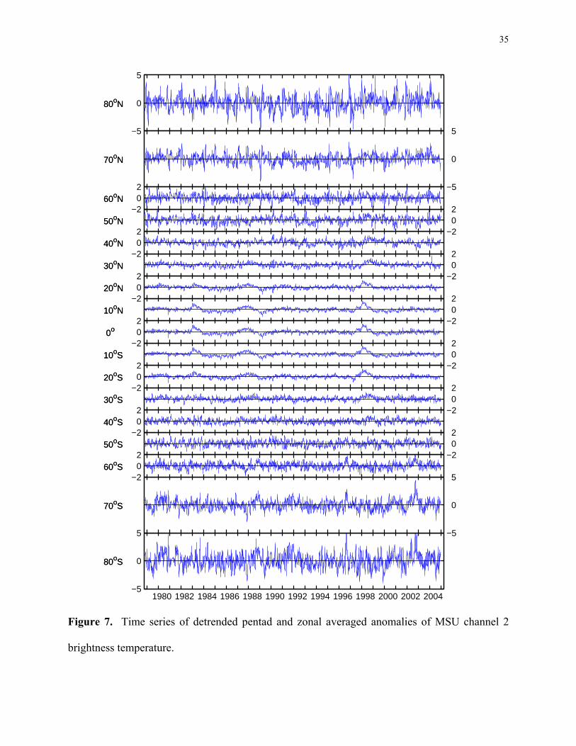
seasonal variations. Figure 7 shows the time series of the anomalies y'(t) for each latitude zone.

They represent real climatic process but all that we can see in these time series are a few well-

known El Niño/La Niña events in low latitudes and noise amplification towards the poles.

5. Latitudinal distribution of trends

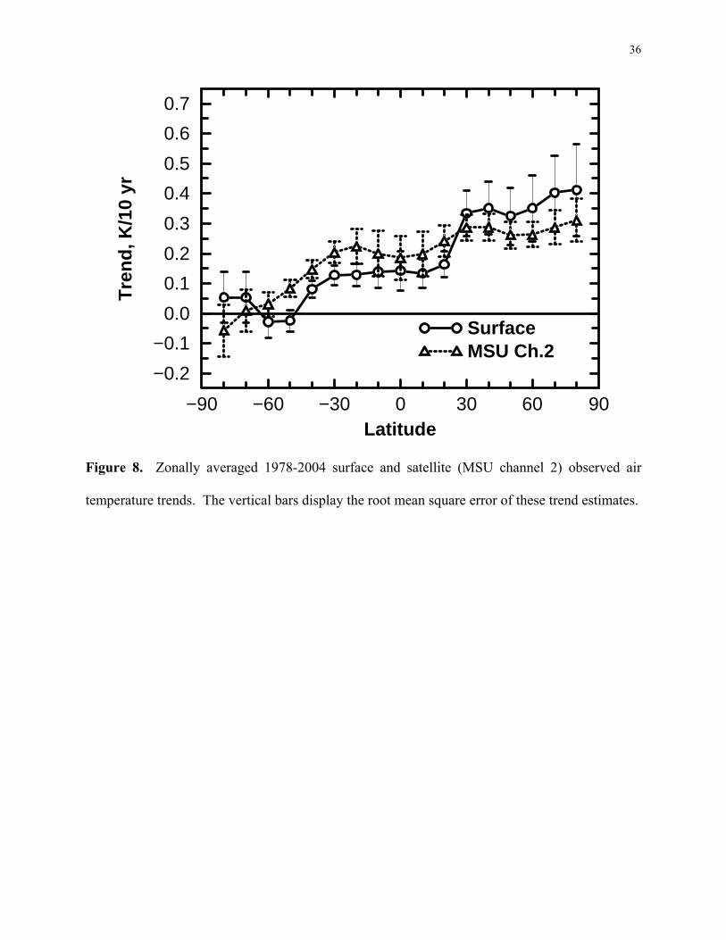
Figure 8 shows the latitudinal distribution of the trend of annual averages based on this

latest calibration and analysis procedure. The observed MSU channel 2 brightness temperature

trend was between +0.2 K/10yr and +0.3 K/10yr north of 30°S, but decreased south of this

latitude until it became a small negative value. The vertical bars in the Figure display the root

mean square error of the trend estimate at each 10° latitude band due to climate variability.

However, uncertainties in inter-satellite calibration can introduce additional errors in these trend

estimates.

For comparison purposes, Figure 8 also displays the trends in the observed surface air

temperature, based on the combined land surface air [Jones and Moberg, 2003] and marine

[Rayner et al., 2003] sea surface temperature anomalies from a 1961-1990 base period. The

same trend estimate for all of Antarctica south of 65°S, land only, is plotted twice at 70°S and

80°S. As for the MSU trend, the vertical bars display the root mean square error of the trend

estimates for surface air temperature based on natural climate variability. These data are less

accurate over data-sparse areas such as the sea-ice-covered oceans and polar regions, which have

17

few permanent land-based meteorological stations. The root mean square errors of the MSU

tropospheric trends and surface trends are greater at high latitudes because of the increased local

temperature variability and the decreased zonal areas, which amplify the variability of zonal

averages at high latitudes [Vinnikov, 1986].

The tropospheric trend obtained from the MSU and the surface air temperature trend have

almost the same global mean of about +0.17 K/10 yr, but display different latitudinal patterns in

Figure 8. At low latitudes, the tropospheric trend exceeds the surface air temperature trend,

whereas the surface warming greatly exceeds the tropospheric warming trend north of 25°N.

This latter feature is consistent with a more stable temperature structure with increasing latitude,

which tends to decouple the surface layer from the troposphere, and is not significantly altered

by the small warming trends. However, the trends have different directions in the Antarctic

region. Due to the high elevation ice sheets, the surface temperature contributions in the MSU

channel 2 brightness temperatures are much larger than 10% so that one would expect to see

similar features in both the MSU and surface data. However, in the 65°S-85°S zone the surface

data over Antarctic continent are only based on a small number of the permanent stations which

are less representative of the Antarctic region than the satellite observations. Of course, as was

discussed earlier, we can speculate that it is reasonable to expect larger differences between the

surface record and MSU channel 2 for regions with lower tropopause heights. To further

examine the physical reasons for the observed patterns, we turn to our best theoretical

understanding of the climate system, which is based on a comprehensive atmosphere-ocean

general circulation model.

Here we use the Geophysical Fluid Dynamics Laboratory (GFDL) climate model

[Manabe et al., 1991; Delworth et al., 2002]. We use these results as an example and expect that

18

most climate models would produce similar trends [Cubasch et al., 2001]. Specifically, we use

ensemble runs of the R30 version of this model, forced by observed changes of CO2 and sulfate

aerosols [Delworth and Knutson, 2000; Delworth et al., 2002]. Three runs of the GFDL model

having different initial states, but with the same forcing, show the 1978-2004 surface warming

trend to be about +0.2 K/10 yr, which is close to the observed surface trend of +0.17 K/10 yr. To

simulate the corresponding MSU channel 2 trend we use the GFDL modeled atmospheric and

surface temperatures, surface pressure, and sea ice thickness as input to the radiative transfer

model of Grody et al. [2004]. The surface emissivity in this computation was assumed to be

0.95 for land and sea ice (thicker than 2 cm) and 0.53 for water surfaces. Also included is the

effect of changing sea ice extent on the emissivity and resulting microwave brightness

temperatures [Swanson, 2003]. Figure 9 shows the 1978-2004 ensemble averaged trend

estimates for the GFDL modeled surface air temperature and simulated MSU channel 2 trends.

Errors in these trend estimates due to the natural variability of climate change are computed

using the 900-year control run of the same model.

The latitudinal dependence of the modeled trends in Figure 9 and the observed trends in

Figure 8 have similar features. As with the observed trends, the modeled surface temperature

trend is also smaller than that of simulated MSU in the low latitudes and larger in the high

latitudes of the Northern Hemisphere. The absence of thermal convection in very cold climatic

conditions appears to decouple the surface temperature and free atmosphere trends. This is why

we do not see polar amplification in the middle troposphere and in the MSU brightness

temperatures. However, the polar amplification in the Northern Hemisphere in the modeled

surface temperature is stronger than in the observed data. As a result, the modeled MSU trend

does not decrease with increasing latitude. Still, the agreement between the observed and

19

modeled MSU trend north of 45°S is remarkable. There is also no cooling trend found in the

modeled temperatures at high latitudes in the Southern Hemisphere. We can speculate that

ozone depletion is responsible for the Antarctic cooling in the free atmosphere [e.g., Thompson

and Solomon, 2002], which is not included in the model. In addition to not including ozone

depletion, many other important radiative forcings are not included such as volcanic eruptions,

indirect effect of aerosols, direct aerosol effects due to black and organic carbons, and the effects

due to land surface changes and many other potential agents capable of changing climate. These

factors may be responsible for the differences between the observed and modeled trends.

However, the largest well understood forcings [Ramaswamy et al., 2001] are included in the

model integrations used here. The indirect effect has very large uncertainties [Ramaswamy et

al., 2001].

Previous work showed larger differences between the climatic trends of temperature

measured by the microwave satellite instruments and those determined from surface observations

[Wallace et al., 2000]. Our improvements in the inter-satellite calibration of the MSU

instruments have resolved much of the difference between the satellite measurements and surface

observations. This consistency between observations has been further strengthened by the

correlation observed with climate models. The high correlation between observations and

modeled results is shown in Fig. 10 by plotting the difference between the surface air

temperature and MSU brightness temperature for both the observed and modeled results of Figs.

8 and 9. The error bars shown for the modeled results were computed from the same 900 year

control run and represents the effect of natural climate variability. Unfortunately, however, error

bars cannot be estimated for the observed trends because of the very short period of observations.

20

However, the similarity of two curves, particularly between latitudes of ±60°, gives us

confidence in both the observations and model results.

We do not see any serious inconsistencies between the 1978-2004 climatic trends

observed by the MSU, surface temperature measurements, and climate model runs. The

agreement between observations and the model give us more confidence in both. Furthermore,

our results suggest a decreased vertical stability of the atmosphere (with the surface warming

faster than the troposphere) in high and middle latitudes and an increasing stability (surface

warming more slowly than the troposphere) at low latitudes, which we also find in model

simulations of contemporary climate change. This result was predicted long ago by climate

models [Manabe and Wetherald, 1975; Hansen et al., 1984] and later found in observations from

the global radiosonde network [Vinnikov et al., 1996]. Although there is much uncertainty in the

forcings used [Ramaswamy et al., 2001], in the model’s response [Cubasch et al., 2001], and in

sampling the observational signal, the fact that the model and observations agree so closely gives

us more confidence in both the observational record and in the model projections of future

climate change.

6. Additional uncertainty in satellite data

Grody et al. [2004] pointed out that if we know that one instrument is much better

calibrated than the others, this instrument could be chosen as an unbiased reference instrument,

i.e., δT = δU = 0. Since we have no such a-priori knowledge, we assumed that one of the

radiometers, NOAA-10, has a zero offset (i.e., δTNOAA-10 = 0.), since this assumption does not

affect the trend estimate. It is possible, however, that one of the instruments is really much better

calibrated than all of the others. In such a case it should be chosen as reference instrument with

the assumption that δT = δU = 0. Using this approach, Table 3 shows the resulting climatic trend

21

in the globally averaged MSU channel 2 brightness temperature under the assumption that the

calibration of one radiometer is error free. Note that all of the trend estimates are within the

range of 0.20 K/10yr to 0.27 K/10yr. It is quite reasonable to expect that the true trend is

somewhere inside of this interval, which is surprisingly small. The current best estimate of the

trend, based on assumption that none of instruments is perfectly calibrated, is 0.20 K/10yr (see

Table 2). It is interesting, however, that all of the adjustment coefficients, δU, given in Table 1

have the same negative sign. It looks as if all nine MSU instruments have channel 2 calibration

nonlinearity biased in the same direction, with the TIROS-N MSU radiometer having the

smallest magnitude of adjustment, δU. By choosing this instrument as reference we obtain a

global trend estimate the same 0.20 K/10yr. It also looks as if the difference between

instruments does not significantly increase the uncertainty in the global climate trend estimates.

Furthermore, none of the instruments being used as reference decreases the global trend estimate

below 0.20 K/10yr.

For completeness, we compare this latest trend of 0.20 K/10yr with the first trend

analysis of MSU channel 2 and AMSU channel 5 by Vinnikov and Grody [2003], which only

considered constant biases (i.e., δU = 0 in (1)) and pre-calibrated the MSU’s using earlier pre-

launch nonlinear coefficients [Mo et al., 1995]. As a result, the global trend was 0.26 K/10yr for

the 24 year period ending in 2002. To obtain accurate comparisons, the Vinnikov and Grody

[2003] technique was applied to the updated 26 years of MSU measurements, which were pre-

calibrated using the latest pre-launch nonlinear coefficients [Mo et al., 2001] used in this paper.

These updated MSU measurements resulted in a different set of constant bias adjustments as well

as a slightly smaller global trend of 0.24 K/10yr. This trend is only a little larger than the 0.20

K/10yr obtained here using the more accurate inter-satellite calibration method [Grody et al.,

22

2004]. However, in addition to providing a more accurate trend, this latest technique

automatically corrects for systematic errors in the pre-launch nonlinear calibration coefficients so

that the results are insensitive to changes in the MSU pre-calibration. In conclusion, we find that

the best estimate of the globally averaged trend of MSU channel 2 is 0.20 K/10yr, with a

standard deviation of 0.05 K/10 yr (see Table 2), which compares very well with the trend

obtained from surface reports.

Acknowledgments. K.Y.V. acknowledges support by NOAA grants COMM NA17EC1483 and

NA06GPO403. P.D.J. was supported by the Office of Science (BER), U.S. Dept. of Energy,

Grant No. DE-FG02-98ER62601. A.R. was supported by National Science Foundation grant

ATM-0313592. The views expressed in this publication are those of the authors and do not

necessarily represent those of NOAA. We thank J. Lanzante, T. Knutson, B. Soden, A. Leetmaa,

J. Sullivan, D. Tarpley, and A. Powell for their useful comments and discussions; and Z. Chang

for initial processing of the satellite data.

23

References

Christy, J. R., and W. B. Norris (2004), What may we conclude about global tropospheric

temperature trends? Geophys. Res. Lett., 31, L06211, doi:10.1029/2003GL019361.

Christy, J. R., R. W. Spencer, and W. D. Braswell (2000), MSU tropospheric temperatures:

Dataset construction and radiosonde comparisons, J. Climate, 17, 1153-1170.

Cubasch, U. et al. (2001), Projections of future climate change, Ch. 9 of IPCC, Climate Change

2001, The Scientific Basis, J. T. Houghton et al., eds., pp. 525-582, Cambridge Univ. Press,

Cambridge, UK.

Delworth, T. L. et al. (2002), Review of simulations of climate variability and change with the

GFDL R30 coupled climate model, Climate Dyn., 19, 555-574.

Delworth, T. L., and T. R. Knutson (2000), Simulation of early 20th Century global warming,

Science, 287, 2246-2250.

Fu, Q., C. M. Johanson, S. G. Warren, and D. J. Seidel (2004), Contribution of stratospheric

cooling to satellite-inferred tropospheric temperature trends, Nature, 429, 55-58.

Fu, Q., and C. M. Johanson (2005), Satellite-derived vertical dependence of tropical tropospheric

temperature trends, Geophys. Res. Lett., 32, L10703, doi:10.1029/2004GL022266.

Grody, N. C., K. Y. Vinnikov, M. D. Goldberg, J. T. Sullivan, and J. D. Tarpley (2004),

Calibration of multi-satellite observations for climatic studies: Microwave Sounding Unit

(MSU), J. Geophys. Res., 109, D24104, doi:10.1029/2004JD005079.

Hansen, J., et al. (1984), Climate sensitivity: Analysis of feedback mechanisms, in Climate

Processes and Climate Sensitivity, J. Hansen and T. Takahashi, eds., AGU Geophys.

Monograph, 29, pp. 130-163, Amer. Geophys. Union, Washington, DC.

24

Ignatov, A., I. Laszlo, E. D. Harrod, K. B. Kidwell, and G. P. Goodrum (2004), Equator crossing

times for NOAA, ERS and EOS sun-synchronous satellites, Int. J. Remote Sensing, 25, 5255-

5266.

Jenkins, G. M., and D. G. Watts (1968), Spectral Analysis and its Applications, Holden Day,

Merrifield, Virginia, pp 132-135.

Jones, P. D., and A. Moberg (2003), Hemispheric and large-scale surface air temperature

variations: An extensive revision and an update to 2001, J. Climate, 16, 206-223.

Manabe S., R. J. Stouffer, M. J. Spelman, and K. Bryan (1991), Transient response of a global

ocean-atmosphere model to gradual changes of atmospheric CO2, Part I: Annual mean

response, J. Climate, 4, 785-818.

Manabe, S., and R. Wetherald (1975), The effect of doubling the CO2 concentration on the

climate of a general circulation model, J. Atmos. Sci., 32, 3-15.

Mears, C. A., M. C. Schabel, and F. J. Wentz (2003), A reanalysis of the MSU channel 2

tropospheric temperature record, J. Climate, 16, 3650-3664.

Mo, T., M. D. Goldberg and D. S. Crosby (2001), Recalibration of the NOAA Microwave

Sounding Unit, J. Geophys. Res., 10, 10,145-10,150.

Mo, T. (1995), A study of the Microwave Sounding Unit on the NOAA-12 satellite, IEEE Trans.

Geosci. Rem. Sens., 33, 1141-1152.

Polyak, I. (1979), Methods for the Analysis of Random Processes and Fields in Climatology, 255

pp., Gidrometeoizdat, Leningrad. (in Russian)

Ramaswamy, V., et al. (2001), Radiative forcing of climate change, Ch. 6 of IPCC, Climate

Change 2001, The Scientific Basis, J. T. Houghton et al., eds., pp. 350-414, Cambridge Univ.

Press, Cambridge, UK.

25

Rayner, N. A., et al. (2003), Global analyses of sea surface temperature, sea ice, and night

marine air temperature since the late nineteenth century, J. Geophys. Res., 108(D14), 4407,

doi:10.1029/2002JD002670.

Swanson, R. E. (2003), Evidence of possible sea-ice influence on Microwave Sounding Unit

tropospheric temperature trends in polar regions, Geophys. Res. Lett., 30,

doi:10.1029/2003GL017938.

Thompson, D. W. J., and S. Solomon (2002), Interpretation of Southern Hemisphere climate

change, Science, 296, 895-899.

Vinnikov, K. Y. (1986), Climate Sensitivity, 224 pp., Gidrometeoizdat, Leningrad. (in Russian)

Vinnikov K. Y., and N. C. Grody (2003), Global warming trend of mean tropospheric

temperature observed by satellites, Science, 302, 269-272.

Vinnikov, K. Y., A. Robock, R. J. Stouffer, and S. Manabe (1996), Vertical patterns of free and

forced climate variations, Geophys. Res. Lett., 23, 1801-1804.

Vinnikov, K. Y., A. Robock, D. J. Cavalieri, and C. L. Parkinson (2002), Analysis of seasonal

cycles in climatic trends with application to satellite observations of sea ice extent, Geophys.

Res. Lett., 29(9), doi:10.1029/2001GL014481.

Wald, A. (1940), The fitting of straight lines if both variables are subject to error, Ann. Math.

Stat., 11, 284-300.

Wallace, J. M. et al. (2000), Reconciling Observations of Global Temperature Change, 106 pp.,

Nat. Acad. Sci., Washington, DC

26

Table 1. Offsets (δT) and parameters (δU) in Eq. (1) used to adjust pentad and 2.5°x2.5°-

averaged observed MSU channel 2 brightness temperatures for ascending and descending orbits.

Satellite δT, K 104·δU, K-1

TIROS-N 0.42 -0.20 NOAA-6 0.06 -0.48 NOAA-7 0.36 -0.33 NOAA-8 -0.12 -0.86 NOAA-9 -0.14 -1.08 NOAA-10 0.00 -0.85 NOAA-11 -0.17 -0.73 NOAA-12 0.29 -0.50 NOAA-14 0.33 -0.55

27

Table 2. 1978-2004 MSU channel 2 brightness temperature trend estimates for eight regions of

the globe, using ordinary and generalized least squares. Number of harmonics used to

approximate seasonal and diurnal cycles in A(t) and B(t) are equal to K=N=M=2, L=1 (see Eq. 5).

Least Squares for Independent Data

Least Squares for Correlated Data

Region

Tmean, K

σ, Kr(τ) τ=12h

Trend, K/10yr

Trend, K/10yr

σTrend, K/10yr

High latitudes 244.6 0.25 0.96 0.19 0.18 0.03 Low latitudes 256.6 0.31 0.99 0.26 0.21 0.07

Global 250.7 0.22 0.98 0.22 0.20 0.05 Antarctic 224.3 1.34 0.99 -0.06 -0.06 0.09

Arctic 237.0 1.33 0.99 0.27 0.31 0.07 Tropical oceans 255.7 0.34 0.96 0.25 0.21 0.06

N. Africa 258.5 0.54 0.93 0.31 0.29 0.06 Tibet 250.2 0.96 0.84 0.32 0.32 0.06

28

Table 3. Global trend (K/10yr) of MSU channel 2 brightness temperature estimates using

different MSU instruments as reference. The column pertaining to overlaps=12 means that all

overlapping observations were used to estimate the calibration adjustment coefficients [Grody et.

al., 2004]. The results based on overlap=8 means that only the 8 longest satellite overlaps were

used in estimating the calibration adjustments [Vinnikov and Grody, 2003].

Overlaps ReferenceMSU 12 8

TIROS-N 0.20 0.20NOAA-6 0.22 0.22NOAA-7 0.22 0.21NOAA-8 0.23 0.24NOAA-9 0.27 0.24NOAA-10 0.26 0.23NOAA-11 0.26 0.23NOAA-12 0.23 0.21NOAA-14 0.24 0.21

29

Figure 1. Representative amplitude spectrum, 222)( iii baF +=ω , showing all of the components up to the second harmonic in the seasonal and diurnal cycles.

πω2

i

)( iF ω

.1,1H

DT

S ==

0 S 2S D D+S

D+2SD-S

D-2S 2D+S

2D+2S 2D-S

2D-2S

2D

30

0 30 60 90 120 150 180 210 240 270 300 330 360Lag, dy

−0.1

0.0

0.1

0.2

0.3

0.4

0.5

0.6

0.7

0.8

0.9

1.0C

orre

latio

nLAG CORRELATION OF PENTAD AVERAGES

MSU Ch.2 Brightness Temperature

30o<|lat|<82.5

o

|lat|<30o

Global 82.5oS−82.5

oN

Antarctic 75−82.5oS

Arctic 75−82.5oN

Ocean 15−25oS

N. AfricaTibet

Figure 2. Empirically estimated lag correlations of pentad-averaged MSU channel 2 brightness

temperatures for eight selected regions. These functions are used in constructing the covariance

matrix (Eq. 10), which is used in the generalized least squares technique (see Eq. 9).

31

|LA

T|>

30o

Mean temperature, K

244 244

246 246

J F M A M J J A S O N D 048

12162024

Loca

l tim

e (H

ours

)

1st diurnal harmonic, K

−.2

0

0

.2


12162024

Loca

l tim

e (H

ours

)

2nd diurnal harmonic, K

−.1

−.1

−.1

−.1

0

0 0

0

0

0

.1

.1 .1


12162024

Loca

l tim

e (H

ours

)

Trend, K/10 yr)

.1

.1.15 .15.2

.2

.25


12162024

|LA

T|<

30o

256 256256.5

256.5

257


12162024

Loca

l tim

e (H

ours

)

−.2

−.2

0

0

.2

.2


12162024

Loca

l tim

e (H

ours

)

−.1

−.1

−.1

−.1

0

0 0

0

0

0

.1.1

.1 .1


12162024

Loca

l tim

e (H

ours

)

.2

.25

.25

.3 .3


12162024

Glo

bal

250

250251251


12162024

Loca

l tim

e (H

ours

)

−.2

−.2

0

0

.2

.2


12162024

Loca

l tim

e (H

ours

)

−.1

−.1

−.1

−.1

0

0 0

0

0

0

.1.1

.1 .1


12162024

Loca

l tim

e (H

ours

)

.2 .2 .2

.25 .25.25


12162024

Ant

arct

ic 220

220230

230


12162024

Loca

l tim

e (H

ours

)

−.1

0

0

0

.1


12162024

Loca

l tim

e (H

ours

)−.4

−.4

−.4

0

0 0

0

0

0

.4

.4

.4

.4


12162024

Loca

l tim

e (H

ours

)

−.4 −.4−.2 −.2

0 0

.2 .2

.4


12162024

Arc

tic

230 230

240240


12162024

Loca

l tim

e (H

ours

)

−.1

0

0

00.1


12162024

Loca

l tim

e (H

ours

)

0

0

0

00

0

.3

.3

.3

.3

.3

.3


12162024

Loca

l tim

e (H

ours

)

.2 .2

.2 .2.4

.4


12162024

Oce

an 1

5−25

o S

255256 256


12162024

Loca

l tim

e (H

ours

)

−.1−.1

0

0

.1 .1


12162024

Loca

l tim

e (H

ours

)

−.1

−.1

−.1

0

0

0

0

0

0.1

.1.1

.1


12162024

Loca

l tim

e (H

ours

)

.2

.2

.25.25

.3

.3


12162024

N. A

fric

a

256 256

258 258260


12162024

Loca

l tim

e (H

ours

)

−1

−.5

−.5

0

0

.5

.5

1


12162024

Loca

l tim

e (H

ours

)

−.2

−.2

−.2

−.2

0

0

0

0

.2

.2

.2

.2.2

.4


12162024

Loca

l tim

e (H

ours

)

.25

.3 .3.3

.35

.35

.4


12162024

Tib

et

250

250

260


12162024

Loca

l tim

e (H

ours

)

−2

−1

−1

0

0

1

1

2


12162024

Loca

l tim

e (H

ours

)

−.4

−.4

−.4

−.4

0

0

0

0.4

.4

.4

.4 .4


12162024

Loca

l tim

e (H

ours

)

.2.2

.3

.3

.3

.4

.4

.5


12162024

Figure 3. Estimates of seasonal and diurnal variations in the multi-year mean temperature, in

the 1st and 2nd harmonics of the diurnal cycle, and in the trend B(t), obtained from ordinary least

squares for independent observations.

32

|LA

T|>

30o

Mean temperature, K

244

244246 246


12162024

Loca

l tim

e (H

ours

)

1st diurnal harmonic, K

−.2

0

0

.2


12162024

Loca

l tim

e (H

ours

)

2nd diurnal harmonic, K

0

0

0

0

0 0


12162024

Loca

l tim

e (H

ours

)

Trend, K/10 yr)

.15 .15

.2.2.25


12162024

|LA

T|<

30o

256.5

256.5

257


12162024

Loca

l tim

e (H

ours

)

−.2

−.2

0

0

.2

.2


12162024

Loca

l tim

e (H

ours

)

0

0

0

0

0

0

.05


12162024

Loca

l tim

e (H

ours

)

.18

.22 .22


12162024

Glo

bal

250 250

251 251


12162024

Loca

l tim

e (H

ours

)

−.2

−.2

0

0

.2

.2


12162024

Loca

l tim

e (H

ours

)

0

0

0

0

0

0.05


12162024

Loca

l tim

e (H

ours

)

.18

.2

.2.22


12162024

Ant

arct

ic

220 220230 230


12162024

Loca

l tim

e (H

ours

)

−.10

0

0

.1


12162024

Loca

l tim

e (H

ours

)

−.1

−.1

0

0

00

0

0

.1

.1


12162024

Loca

l tim

e (H

ours

)

−.4−.2 −.2

0

0


12162024

Arc

tic

230 230240 240


12162024

Loca

l tim

e (H

ours

)

−.1

0

0

0

0

.1


12162024

Loca

l tim

e (H

ours

)

−.1

−.1

0

0

0

0

.1

.1


12162024

Loca

l tim

e (H

ours

)

.2 .2.2.2.4 .4 .6 .6


12162024

Oce

an 1

5−25

o S

255

256256


12162024

Loca

l tim

e (H

ours

)

−.1 −.1

0

0

.1 .1


12162024

Loca

l tim

e (H

ours

)

−.05 −.05

−.05

0

0

0

0

0

.05

.05

.05

.05


12162024

Loca

l tim

e (H

ours

)

.15

.2

.2


12162024

N. A

fric

a

256

258 258

260


12162024

Loca

l tim

e (H

ours

)

−1

−.5

−.5

0

0

.5

.51


12162024

Loca

l tim

e (H

ours

)

−.2−.2

−.2−.2

0

0

0

0

.2

.2

.2

.2


12162024

Loca

l tim

e (H

ours

)

.25.3 .3

.3


12162024

Tib

et

250 250260


12162024

Loca

l tim

e (H

ours

)

−2

−1

−1

0

0

1

12


12162024

Loca

l tim

e (H

ours

)

−.4

−.4

−.4

−.4

0

0

0

0.4

.4

.4

.4 .4


12162024

Loca

l tim

e (H

ours

)

.2

.3

.3

.4 .4

.5


12162024

Figure 4. Estimates of seasonal and diurnal variations in the multi-year mean temperature, in

the 1st and 2nd harmonics of diurnal cycle, and in the trend B(t), obtained from generalized least

squares for correlated observations.

33

1978 1980 1982 1984 1986 1988 1990 1992 1994 1996 1998 2000 2002 2004−0.1

0.0

0.1

Tem

pera

ture

(K

)

TN

N6

N7

N8N9

N10

N11 N12

N14

Figure 5. Effect of changes in Equator crossing time on computed daily averages in global and

pentad averaged MSU channel 2 brightness temperatures observed from NOAA satellites. This

plot only contains the contributions from the second harmonic components, with the first

harmonic seasonal and diurnal components removed.

34

1980 1982 1984 1986 1988 1990 1992 1994 1996 1998 2000 2002 2004 215220225230235

80oS

230

240

70oS

235240245

60oS

24024550oS

24525040oS

250255

30oS 255258

20oS 256259

10oS 257260

0o 257260

10oN 255260

20oN 250255260

30oN

245250255260

40oN

240245250255

50oN

240

250

60oN

230

240

250

70oN

230

240

250

80oN

Figure 6. Expected value and anomalies combined of the pentad and zonally averaged MSU

channel 2 brightness temperature. The nearly horizontal lines are the climatic trend in annual

averages.

35

1980 1982 1984 1986 1988 1990 1992 1994 1996 1998 2000 2002 2004 −5

0

5

80oS80oS

−5

0

5

70oS70oS

−2

02

60oS60oS −2 0 2

50oS50oS −2

02

40oS40oS −2 0 2

30oS30oS −2

02

20oS20oS −2 0 2

10oS10oS −2

02

0o 0o −2 0 2

10oN10oN −2

02

20oN20oN −2 0 2

30oN30oN −2

02

40oN40oN −2 0 2

50oN50oN −2

02

60oN60oN −5

0

5

70oN70oN

−5

0

5

80oN80oN

Figure 7. Time series of detrended pentad and zonal averaged anomalies of MSU channel 2

brightness temperature.

36

−90 −60 −30 0 30 60 90Latitude

−0.2

−0.1

0.0

0.1

0.2

0.3

0.4

0.5

0.6

0.7T

rend

, K/1

0 yr

Surface MSU Ch.2

Figure 8. Zonally averaged 1978-2004 surface and satellite (MSU channel 2) observed air

temperature trends. The vertical bars display the root mean square error of these trend estimates.

37

−90 −60 −30 0 30 60 90Latitude

−0.2

−0.1

0.0

0.1

0.2

0.3

0.4

0.5

0.6

0.7T

rend

, K/1

0 yr

Surface MSU Ch.2

Figure 9. Zonally averaged 1978-2004 surface and satellite (MSU channel 2) modeled air

temperature trends, from the GFDL R-30 climate model ensemble run forced by changes in CO2

and sulfate aerosol [Delworth and Knutson, 2000; Delworth et al., 2002]. The vertical bars

display the root mean square errors of these trend estimates.

38

−90 −60 −30 0 30 60 90Latitude

−0.2

−0.1

0.0

0.1

0.2

0.3

0.4

0.5

0.6

0.7T

rend

Diff

eren

ce, K

/10

yr ModeledObserved

Figure 10. Differences between 1978-2004 trends in surface and troposphere air temperatures

based on observations (Observed) and climate model (Modeled), i.e., difference of plots in

Figures 8 and 9. These differences have different signs in low and high latitudes. Root mean

errors of modeled differences (shown with vertical bars) were estimated from a 900-year control

run of the same model.

Documents

Temperature Trends at the Surface and in the Troposphere