Embed Size (px)
Citation preview
arX
iv:1
712.
0661
2v1
[as
tro-
ph.H
E]
18
Dec
201
7Publ. Astron. Soc. Japan (2014) 00(0), 1–27
doi: 10.1093/pasj/xxx000
1
Temperature Structure in the Perseus Cluster
Core Observed with Hitomi ∗
Hitomi Collaboration, Felix AHARONIAN1,2,3 , Hiroki AKAMATSU4 , Fumie
AKIMOTO5 , Steven W. ALLEN6,7,8, Lorella ANGELINI9 , Marc AUDARD10,
Hisamitsu AWAKI11, Magnus AXELSSON12 , Aya BAMBA13,14, Marshall W.
BAUTZ15, Roger BLANDFORD6,7,8 , Laura W. BRENNEMAN16 , Gregory V.
BROWN17 , Esra BULBUL15, Edward M. CACKETT18 , Maria CHERNYAKOVA1 ,
Meng P. CHIAO9, Paolo S. COPPI19,20 , Elisa COSTANTINI4 , Jelle DE PLAA4,
Cor P. DE VRIES4 , Jan-Willem DEN HERDER4, Chris DONE21, Tadayasu
DOTANI22 , Ken EBISAWA22 , Megan E. ECKART9 , Teruaki ENOTO23,24 , Yuichiro
EZOE25 , Andrew C. FABIAN26, Carlo FERRIGNO10 , Adam R. FOSTER16 ,
Ryuichi FUJIMOTO27 , Yasushi FUKAZAWA28 , Maki FURUKAWA29 , Akihiro
FURUZAWA30 , Massimiliano GALEAZZI31 , Luigi C. GALLO32, Poshak
GANDHI33, Margherita GIUSTINI4 , Andrea GOLDWURM34,35 , Liyi GU4, Matteo
GUAINAZZI36 , Yoshito HABA37, Kouichi HAGINO38 , Kenji HAMAGUCHI9,39 ,
Ilana M. HARRUS9,39 , Isamu HATSUKADE40 , Katsuhiro HAYASHI22,41 ,
Takayuki HAYASHI41 , Kiyoshi HAYASHIDA42 , Junko S. HIRAGA43 , Ann
HORNSCHEMEIER9 , Akio HOSHINO44 , John P. HUGHES45 , Yuto ICHINOHE25 ,
Ryo IIZUKA22 , Hajime INOUE46, Yoshiyuki INOUE22, Manabu ISHIDA22 , Kumi
ISHIKAWA22 , Yoshitaka ISHISAKI25 , Masachika IWAI22, Jelle KAASTRA4,47,
Tim KALLMAN9 , Tsuneyoshi KAMAE13 , Jun KATAOKA48, Yuichi KATO13,
Satoru KATSUDA49 , Nobuyuki KAWAI50 , Richard L. KELLEY9 , Caroline A.
KILBOURNE9 , Takao KITAGUCHI28 , Shunji KITAMOTO44 , Tetsu KITAYAMA51 ,
Takayoshi KOHMURA38 , Motohide KOKUBUN22 , Katsuji KOYAMA52 , Shu
KOYAMA22 , Peter KRETSCHMAR53 , Hans A. KRIMM54,55 , Aya KUBOTA56,
Hideyo KUNIEDA41 , Philippe LAURENT34,35 , Shiu-Hang LEE23, Maurice A.
LEUTENEGGER9 , Olivier LIMOUSIN35 , Michael LOEWENSTEIN9,57 , Knox S.
LONG58, David LUMB36, Greg MADEJSKI6 , Yoshitomo MAEDA22, Daniel
MAIER34,35 , Kazuo MAKISHIMA59 , Maxim MARKEVITCH9 , Hironori
MATSUMOTO42 , Kyoko MATSUSHITA29 , Dan MCCAMMON60 , Brian R.
MCNAMARA61 , Missagh MEHDIPOUR4 , Eric D. MILLER15 , Jon M. MILLER62 ,
Shin MINESHIGE23 , Kazuhisa MITSUDA22 , Ikuyuki MITSUISHI41 , Takuya
MIYAZAWA63 , Tsunefumi MIZUNO28,64 , Hideyuki MORI9, Koji MORI40, Koji
MUKAI9,39, Hiroshi MURAKAMI65 , Richard F. MUSHOTZKY57 , Takao
NAKAGAWA22 , Hiroshi NAKAJIMA42 , Takeshi NAKAMORI66 , Shinya
NAKASHIMA59 , Kazuhiro NAKAZAWA13,14 , Kumiko K. NOBUKAWA67 ,
Masayoshi NOBUKAWA68 , Hirofumi NODA69,70, Hirokazu ODAKA6, Takaya
OHASHI25 , Masanori OHNO28, Takashi OKAJIMA9 , Naomi OTA67, Masanobu
OZAKI22, Frits PAERELS71 , Stephane PALTANI10 , Robert PETRE9 , Ciro
c© 2014. Astronomical Society of Japan.
2 Publications of the Astronomical Society of Japan, (2014), Vol. 00, No. 0
PINTO26 , Frederick S. PORTER9 , Katja POTTSCHMIDT9,39 , Christopher S.
REYNOLDS57 , Samar SAFI-HARB72 , Shinya SAITO44 , Kazuhiro SAKAI9, Toru
SASAKI29 , Goro SATO22, Kosuke SATO29, Rie SATO22, Makoto SAWADA73 ,
Norbert SCHARTEL53 , Peter J. SERLEMTSOS9 , Hiromi SETA25, Megumi
SHIDATSU59 , Aurora SIMIONESCU22 , Randall K. SMITH16 , Yang SOONG9 ,
Łukasz STAWARZ74 , Yasuharu SUGAWARA22 , Satoshi SUGITA50 , Andrew
SZYMKOWIAK20 , Hiroyasu TAJIMA5 , Hiromitsu TAKAHASHI28 , Tadayuki
TAKAHASHI22 , Shinıchiro TAKEDA63, Yoh TAKEI22, Toru TAMAGAWA75 ,
Takayuki TAMURA22, Takaaki TANAKA52, Yasuo TANAKA76,22, Yasuyuki T.
TANAKA28, Makoto S. TASHIRO77 , Yuzuru TAWARA41, Yukikatsu TERADA77,
Yuichi TERASHIMA11 , Francesco TOMBESI9,78,79 , Hiroshi TOMIDA22 , Yohko
TSUBOI49 , Masahiro TSUJIMOTO22 , Hiroshi TSUNEMI42 , Takeshi Go TSURU52,
Hiroyuki UCHIDA52, Hideki UCHIYAMA80 , Yasunobu UCHIYAMA44 , Shutaro
UEDA22, Yoshihiro UEDA23, Shinıchiro UNO81, C. Megan URRY20, Eugenio
URSINO31 , Shin WATANABE22 , Norbert WERNER82,83,28 , Dan R. WILKINS6 ,
Brian J. WILLIAMS58 , Shinya YAMADA25 , Hiroya YAMAGUCHI9,57 , Kazutaka
YAMAOKA5,41 , Noriko Y. YAMASAKI22 , Makoto YAMAUCHI40 , Shigeo
YAMAUCHI67 , Tahir YAQOOB9,39 , Yoichi YATSU50 , Daisuke YONETOKU27 , Irina
ZHURAVLEVA6,7 , Abderahmen ZOGHBI62 ,
1Dublin Institute for Advanced Studies, 31 Fitzwilliam Place, Dublin 2, Ireland2Max-Planck-Institut fur Kernphysik, P.O. Box 103980, 69029 Heidelberg, Germany3Gran Sasso Science Institute, viale Francesco Crispi, 7 67100 L’Aquila (AQ), Italy4SRON Netherlands Institute for Space Research, Sorbonnelaan 2, 3584 CA Utrecht, The
Netherlands5Institute for Space-Earth Environmental Research, Nagoya University, Furo-cho, Chikusa-ku,
Nagoya, Aichi 464-86016Kavli Institute for Particle Astrophysics and Cosmology, Stanford University, 452 Lomita Mall,
Stanford, CA 94305, USA7Department of Physics, Stanford University, 382 Via Pueblo Mall, Stanford, CA 94305, USA8SLAC National Accelerator Laboratory, 2575 Sand Hill Road, Menlo Park, CA 94025, USA9NASA, Goddard Space Flight Center, 8800 Greenbelt Road, Greenbelt, MD 20771, USA10Department of Astronomy, University of Geneva, ch. d’Ecogia 16, CH-1290 Versoix,
Switzerland11Department of Physics, Ehime University, Bunkyo-cho, Matsuyama, Ehime 790-857712Department of Physics and Oskar Klein Center, Stockholm University, 106 91 Stockholm,
Sweden13Department of Physics, The University of Tokyo, 7-3-1 Hongo, Bunkyo-ku, Tokyo 113-003314Research Center for the Early Universe, School of Science, The University of Tokyo, 7-3-1
Hongo, Bunkyo-ku, Tokyo 113-003315Kavli Institute for Astrophysics and Space Research, Massachusetts Institute of Technology,
77 Massachusetts Avenue, Cambridge, MA 02139, USA16Smithsonian Astrophysical Observatory, 60 Garden St., MS-4. Cambridge, MA 02138, USA17Lawrence Livermore National Laboratory, 7000 East Avenue, Livermore, CA 94550, USA18Department of Physics and Astronomy, Wayne State University, 666 W. Hancock St, Detroit,
MI 48201, USA19Department of Astronomy, Yale University, New Haven, CT 06520-8101, USA20Department of Physics, Yale University, New Haven, CT 06520-8120, USA21Centre for Extragalactic Astronomy, Department of Physics, University of Durham, South
Publications of the Astronomical Society of Japan, (2014), Vol. 00, No. 0 3
Road, Durham, DH1 3LE, UK22Japan Aerospace Exploration Agency, Institute of Space and Astronautical Science, 3-1-1
Yoshino-dai, Chuo-ku, Sagamihara, Kanagawa 252-521023Department of Astronomy, Kyoto University, Kitashirakawa-Oiwake-cho, Sakyo-ku, Kyoto
606-850224The Hakubi Center for Advanced Research, Kyoto University, Kyoto 606-830225Department of Physics, Tokyo Metropolitan University, 1-1 Minami-Osawa, Hachioji, Tokyo
192-039726Institute of Astronomy, University of Cambridge, Madingley Road, Cambridge, CB3 0HA, UK27Faculty of Mathematics and Physics, Kanazawa University, Kakuma-machi, Kanazawa,
Ishikawa 920-119228School of Science, Hiroshima University, 1-3-1 Kagamiyama, Higashi-Hiroshima 739-852629Department of Physics, Tokyo University of Science, 1-3 Kagurazaka, Shinjuku-ku, Tokyo
162-860130Fujita Health University, Toyoake, Aichi 470-119231Physics Department, University of Miami, 1320 Campo Sano Dr., Coral Gables, FL 33146,
USA32Department of Astronomy and Physics, Saint Mary’s University, 923 Robie Street, Halifax,
NS, B3H 3C3, Canada33Department of Physics and Astronomy, University of Southampton, Highfield, Southampton,
SO17 1BJ, UK34Laboratoire APC, 10 rue Alice Domon et Leonie Duquet, 75013 Paris, France35CEA Saclay, 91191 Gif sur Yvette, France36European Space Research and Technology Center, Keplerlaan 1 2201 AZ Noordwijk, The
Netherlands37Department of Physics and Astronomy, Aichi University of Education, 1 Hirosawa,
Igaya-cho, Kariya, Aichi 448-854338Department of Physics, Tokyo University of Science, 2641 Yamazaki, Noda, Chiba,
278-851039Department of Physics, University of Maryland Baltimore County, 1000 Hilltop Circle,
Baltimore, MD 21250, USA40Department of Applied Physics and Electronic Engineering, University of Miyazaki, 1-1
Gakuen Kibanadai-Nishi, Miyazaki, 889-219241Department of Physics, Nagoya University, Furo-cho, Chikusa-ku, Nagoya, Aichi 464-860242Department of Earth and Space Science, Osaka University, 1-1 Machikaneyama-cho,
Toyonaka, Osaka 560-004343Department of Physics, Kwansei Gakuin University, 2-1 Gakuen, Sanda, Hyogo 669-133744Department of Physics, Rikkyo University, 3-34-1 Nishi-Ikebukuro, Toshima-ku, Tokyo
171-850145Department of Physics and Astronomy, Rutgers University, 136 Frelinghuysen Road,
Piscataway, NJ 08854, USA46Meisei University, 2-1-1 Hodokubo, Hino, Tokyo 191-850647Leiden Observatory, Leiden University, PO Box 9513, 2300 RA Leiden, The Netherlands48Research Institute for Science and Engineering, Waseda University, 3-4-1 Ohkubo,
Shinjuku, Tokyo 169-855549Department of Physics, Chuo University, 1-13-27 Kasuga, Bunkyo, Tokyo 112-855150Department of Physics, Tokyo Institute of Technology, 2-12-1 Ookayama, Meguro-ku, Tokyo
152-855051Department of Physics, Toho University, 2-2-1 Miyama, Funabashi, Chiba 274-851052Department of Physics, Kyoto University, Kitashirakawa-Oiwake-Cho, Sakyo, Kyoto
606-8502
4 Publications of the Astronomical Society of Japan, (2014), Vol. 00, No. 0
53European Space Astronomy Center, Camino Bajo del Castillo, s/n., 28692 Villanueva de la
Canada, Madrid, Spain54Universities Space Research Association, 7178 Columbia Gateway Drive, Columbia, MD
21046, USA55National Science Foundation, 4201 Wilson Blvd, Arlington, VA 22230, USA56Department of Electronic Information Systems, Shibaura Institute of Technology, 307
Fukasaku, Minuma-ku, Saitama, Saitama 337-857057Department of Astronomy, University of Maryland, College Park, MD 20742, USA58Space Telescope Science Institute, 3700 San Martin Drive, Baltimore, MD 21218, USA59Institute of Physical and Chemical Research, 2-1 Hirosawa, Wako, Saitama 351-019860Department of Physics, University of Wisconsin, Madison, WI 53706, USA61Department of Physics and Astronomy, University of Waterloo, 200 University Avenue West,
Waterloo, Ontario, N2L 3G1, Canada62Department of Astronomy, University of Michigan, 1085 South University Avenue, Ann
Arbor, MI 48109, USA63Okinawa Institute of Science and Technology Graduate University, 1919-1 Tancha,
Onna-son Okinawa, 904-049564Hiroshima Astrophysical Science Center, Hiroshima University, Higashi-Hiroshima,
Hiroshima 739-852665Faculty of Liberal Arts, Tohoku Gakuin University, 2-1-1 Tenjinzawa, Izumi-ku, Sendai,
Miyagi 981-319366Faculty of Science, Yamagata University, 1-4-12 Kojirakawa-machi, Yamagata, Yamagata
990-856067Department of Physics, Nara Women’s University, Kitauoyanishi-machi, Nara, Nara
630-850668Department of Teacher Training and School Education, Nara University of Education,
Takabatake-cho, Nara, Nara 630-852869Frontier Research Institute for Interdisciplinary Sciences, Tohoku University, 6-3
Aramakiazaaoba, Aoba-ku, Sendai, Miyagi 980-857870Astronomical Institute, Tohoku University, 6-3 Aramakiazaaoba, Aoba-ku, Sendai, Miyagi
980-857871Astrophysics Laboratory, Columbia University, 550 West 120th Street, New York, NY 10027,
USA72Department of Physics and Astronomy, University of Manitoba, Winnipeg, MB R3T 2N2,
Canada73Department of Physics and Mathematics, Aoyama Gakuin University, 5-10-1 Fuchinobe,
Chuo-ku, Sagamihara, Kanagawa 252-525874Astronomical Observatory of Jagiellonian University, ul. Orla 171, 30-244 Krakow, Poland75RIKEN Nishina Center, 2-1 Hirosawa, Wako, Saitama 351-019876Max-Planck-Institut fur extraterrestrische Physik, Giessenbachstrasse 1, 85748 Garching ,
Germany77Department of Physics, Saitama University, 255 Shimo-Okubo, Sakura-ku, Saitama,
338-857078Department of Physics, University of Maryland Baltimore County, 1000 Hilltop Circle,
Baltimore, MD 21250, USA79Department of Physics, University of Rome “Tor Vergata”, Via della Ricerca Scientifica 1,
I-00133 Rome, Italy80Faculty of Education, Shizuoka University, 836 Ohya, Suruga-ku, Shizuoka 422-852981Faculty of Health Sciences, Nihon Fukushi University , 26-2 Higashi Haemi-cho, Handa,
Aichi 475-001282MTA-Eotvos University Lendulet Hot Universe Research Group, Pazmany Peter setany 1/A,
Publications of the Astronomical Society of Japan, (2014), Vol. 00, No. 0 5
Budapest, 1117, Hungary83Department of Theoretical Physics and Astrophysics, Faculty of Science, Masaryk
University, Kotlarska 2, Brno, 611 37, Czech Republic
∗E-mail: [email protected]
Received ; Accepted
Abstract
The present paper investigates the temperature structure of the X-ray emitting plasma in
the core of the Perseus cluster using the 1.8–20.0 keV data obtained with the Soft X-ray
Spectrometer (SXS) onboard the Hitomi Observatory. A series of four observations were car-
ried out, with a total effective exposure time of 338 ks and covering a central region ∼ 7′ in
diameter. The SXS was operated with an energy resolution of ∼5 eV (full width at half max-
imum) at 5.9 keV. Not only fine structures of K-shell lines in He-like ions but also transitions
from higher principal quantum numbers are clearly resolved from Si through Fe. This enables
us to perform temperature diagnostics using the line ratios of Si, S, Ar, Ca, and Fe, and to
provide the first direct measurement of the excitation temperature and ionization temperature
in the Perseus cluster. The observed spectrum is roughly reproduced by a single temperature
thermal plasma model in collisional ionization equilibrium, but detailed line ratio diagnostics
reveal slight deviations from this approximation. In particular, the data exhibit an apparent
trend of increasing ionization temperature with increasing atomic mass, as well as small differ-
ences between the ionization and excitation temperatures for Fe, the only element for which
both temperatures can be measured. The best-fit two-temperature models suggest a combi-
nation of 3 and 5 keV gas, which is consistent with the idea that the observed small deviations
from a single temperature approximation are due to the effects of projection of the known
radial temperature gradient in the cluster core along the line of sight. Comparison with the
Chandra/ACIS and the XMM-Newton/RGS results on the other hand suggests that additional
lower-temperature components are present in the ICM but not detectable by Hitomi SXS given
its 1.8–20 keV energy band.
Key words: galaxies: clusters: individual (Perseus) — X-rays: galaxies: clusters — methods: observa-
tional
1 Introduction
The X-ray emitting hot intracluster medium (ICM) dominates
the baryonic mass in galaxy clusters, and its thermodynami-
cal properties are crucial for studying the evolution of large-
scale structure in the Universe. Discontinuities in the ICM
temperature and density profiles reveal ongoing cluster merg-
ers (Markevitch et al. 2000; Vikhlinin et al. 2001; Markevitch
& Vikhlinin 2007; Akamatsu & Kawahara 2013), while the
pressure profiles in the cluster outskirts are also key to under-
standing their growth (Arnaud et al. 2010; Simionescu et al.
2011; Planck Collaboration et al. 2013; Simionescu et al. 2017).
The thermodynamical properties of the dense ICM at the cen-
ters of so-called “cool-core” clusters are even more complex;
despite the fact that radiative cooling in these regions should
∗ Corresponding authors are Shinya NAKASHIMA, Kyoko MATSUSHITA,
Aurora SIMIONESCU, Mark BAUTZ, Kazuhiro NAKAZAWA, Takashi
OKAJIMA, and Noriko YAMASAKI
be very efficient, stars are being formed at a rate smaller than
that expected from the amount of hot ICM (e.g., Peterson et al.
2003). The heating mechanism responsible for compensating
the radiative cooling is under debate, and various ideas have
been proposed, such as feedback from the active galactic nu-
clei (AGN) in the brightest cluster galaxies (e.g., McNamara &
Nulsen 2007), energy transfer from moving member galaxies
(e.g, Makishima et al. 2001; Gu et al. 2013), and cosmic-ray
streaming with Alfven waves (e.g., Fujita et al. 2013). While
less effective than expected, some radiative cooling likely does
occur, and the presence of multi-phase ICM in cool-core clus-
ters is also reported (Fukazawa et al. 1994; Sanders & Fabian
2007; Takahashi et al. 2009; Gu et al. 2012; Sanders et al.
2016; Pinto et al. 2016).
To date, temperature measurements of the ICM have been
mainly performed by fitting broad-band spectra (typically 0.5–
10.0 keV band) obtained from X-ray CCDs. Because of
6 Publications of the Astronomical Society of Japan, (2014), Vol. 00, No. 0
the moderate energy resolution of this type of spectrometers,
temperatures are mainly determined by shapes of the contin-
uum and the Fe L-shell lines complex. However, the con-
tinuum shape is subject to uncertainties due to background
modeling and/or effective area calibration (e.g., de Plaa et al.
2007; Leccardi & Molendi 2008; Nevalainen et al. 2010;
Schellenberger et al. 2015).
An independent estimate of the gas temperature can be ob-
tained from the flux ratios of various emission lines, the so-
called line ratio diagnostic; a ratio between different transitions
in the same ion such as Lyα-to-Lyβ indicates the excitation tem-
perature, and a ratio of lines from different ionization stages
such as Heα-to-Lyα represents the ion fraction (also referred
to as the ionization temperature). These temperatures should
match the temperature from the continuum shape when the ob-
served plasma is truly single temperature in collisional ioniza-
tion equilibrium (CIE). If there is a disagreement between those
temperatures, deviation from a single CIE plasma is suggested:
multi-temperature and/or non-equilibrium ionization (NEI). For
instance, Matsushita et al. (2002) utilized the Si and S K-shell
lines to measure the temperature profile in M 87. Ratios of K-
shell lines from Fe were used for the Ophiuchus Cluster (Fujita
et al. 2008), the Coma Cluster (Sato et al. 2011) and A754
(Inoue et al. 2016). In practice, this method has been applied
to a relatively small number of lines because of line blending
and because only the fluxes of the strongest lines are free from
uncertainties in the exact continuum calibration and background
subtraction.
The XMM-Newton Reflection Grating Spectrometers (RGS)
offer higher spectral resolution and enable us to perform diag-
nostics with O K-shell and Fe L-shell lines, which are sensi-
tive to the temperature range of kT < 1 keV (e.g., Pinto et al.
2016). However, the energy band of the RGS is limited to en-
ergies below 2 keV, and the energy resolution is degraded for
diffuse sources due to the dispersive and slit-less nature of these
spectrometers. Therefore, observations with a non-dispersive
high-resolution spectrometer covering a broad energy band are
desired for a precise characterization of the multi-temperature
structure in the ICM.
The Hitomi satellite launched on February 2016 performed
the first cluster observation of this kind, using its Soft X-
ray Spectrometer (SXS). This non-dispersive microcalorimeter
achieved spectral resolution of ∼5 eV in orbit (Porter et al.
2017), and observed the core of the Perseus cluster as its first
light target. In the observed region, fine ICM substructures such
as bubbles, ripples, and weak shock fronts were previously re-
vealed by deep Chandra imaging (Fabian et al. 2011, and refer-
ences therein). These features are thought to be due to the activ-
ity of the AGN in the cD galaxy NGC 1275, which is pumping
out relativistic electrons that disturb and heat the surrounding X-
ray gas. The presence of multiple phases structure in the ICM
spanning a range of temperatures between kT = 0.5− 8 keV is
also reported (Sanders & Fabian 2007; Pinto et al. 2016).
The first measurement of Doppler shifts and broadening of
the Fe-K emission lines from the Hitomi first-light data, re-
ported in Hitomi Collaboration (2016) (hereafter the First pa-
per), revealed that the line-of-sight velocity dispersion of the
ICM in the core regions is unexpectedly low and subsonic.
Constraints on an unidentified feature at 3.5 keV suggested to
originate from dark matter (e.g., Bulbul et al. 2014) are de-
scribed by Hitomi Collaboration (2017). Using the full set
of the Perseus data and the latest calibration, we have per-
formed X-ray spectroscopy over the full Hitomi SXS band
and report a series of follow-up papers. In this paper, we
concentrate on measurements of the temperature structure in
the cluster core. The high spectral resolution of the SXS al-
lowed us to estimate the gas temperature based on seventeen
independent line ratios from various chemical elements (Si
through Fe). Companion papers report results on the metal
abundances (Hitomi Collaboration 2017a, henceforth the Z pa-
per), velocity fields (Hitomi Collaboration 2017b, the V pa-
per), properties of the AGN in NGC1275 (Hitomi Collaboration
2017c, the AGN paper), the atomic code comparison (Hitomi
Collaboration 2017d, the Atomic paper), and the detection of
resonance scattering (Hitomi Collaboration 2017e, the RS pa-
per).
Throughout this paper, we assume a cluster redshift of
0.017284 (see Appendix 1 of the V paper) and a Hubble con-
stant of 70 km s−1 Mpc−1. Therefore, 1′ corresponds to the
physical scale of 21 kpc. We use the 68% (1σ) confidence level
for errors, but upper and lower limits are shown at the 99.7%
(3σ) confidence level. X-ray energies in spectra are denoted at
the observed (hence redshifted) frame rather than the object’s
rest-frame.
2 Observation and Data Reduction
2.1 Hitomi Observation
We observed the Perseus cluster four times with Hitomi/SXS
during the commissioning phase in 2016 February and March
(Table 1). The aim points of each observation are shown in
Figure 1. The first light observation of Hitomi (obs1), is offset
by ∼ 3′ from the center of the Perseus cluster because the atti-
tude control system was not commissioned at that time. In the
next observation (obs2), the pointing direction was adjusted so
that the Perseus core was in the SXS field-of-view (FoV). The
same region was observed again after extension of the Hitomi
Hard X-ray Detector’s optical bench (obs3). The obs3 is divided
into the three sequential data sets (100040030, 100040040, and
100040050) solely for convenience in pipeline processing. In
the final observation (obs4), the aim point was fine-tuned again
to place the Perseus core at the center of the SXS FoV.
Publications of the Astronomical Society of Japan, (2014), Vol. 00, No. 0 7
The SXS sensor is a 6× 6 pixel array (Kelley et al. 2017).
Combined with the X-ray focusing mirror (Okajima et al. 2016),
the SXS has a 3′ × 3′ FoV with an angular resolution of 1.2′
(half power diameter). One corner pixel is always illuminated
by a dedicated 55Fe source to track the gain variation with de-
tector temperature, and is not used for astrophysical spectra.
The SXS achieved the unprecedented energy resolution of 5 eV
(full width at half maximum) at 5.9 keV in orbit (Porter et al.
2017). The required energy bandpass of the SXS was 0.3–12
keV. During the early-mission observations discussed here, a
gate valve remained closed to minimize the risk of contamina-
tion from outgassing in the spacecraft. The valve includes a Be
window that absorbs most X-rays below 2 keV (Eckart et al.
2017).
The other instruments on Hitomi (Takahashi et al. 2017)
were not yet operational during most or all of the Perseus ob-
servations described here.
2.2 Hitomi Data Reduction
We used the cleaned event list provided by the pipeline process-
ing version 03.01.006.007, and applied the additional screen-
ing described below using the HEAsoft version 6.21, Hitomi
software version 6, and Hitomi calibration database version 71
(Angelini et al. 2017).
The SXS recorded signals up to 32 keV, but the standard
pipeline processing reduces the energy coverage to the 0–
16 keV band in order to achieve a sufficiently fine energy bin
with the realistic number of channels in the nominal energy
band (32768 bins with 0.5 eV bin−1). However, the SXS was
sensitive to bright sources above 16 keV because of its very low
non-X-ray background (Kilbourne et al. 2017). We thus used
a coarser bin size of 1.0 eV bin−1 to extend the energy cover-
age up to 32 keV instead. This was technically achieved by the
sxsextend ftools task. We confirmed that choosing the coarser
bin size has no impact on our analysis due to intrinsic thermal
and velocity broadening of lines.
We then applied event screening based on a pulse rise time
versus energy relationship tuned for the wider energy cover-
age2. We also selected only high primary grade events, for
which arrival time between signal pulses was sufficiently large
and hence the best spectroscopic performance was achieved.
The branching ratio to other grades was less than 2% for the
Perseus observations, so this grade selection hardly reduced the
effective exposure.
Since the in-flight calibration of the SXS is limited, there
is uncertainty of the gain scale especially at energies far from
5.9 keV. In addition, the SXS was not in thermal equilibrium
1 See https://heasarc.gsfc.nasa.gov/docs/hitomi/analysis for the Hitomi soft-
ware and calibration database2 See the Hitomi data reduction guide for details
(https://heasarc.gsfc.nasa.gov/docs/hitomi/analysis).
during obs1 and obs2, and thus a ∼2 eV gain shift was seen
even at 5.9 keV (Fujimoto et al. 2017). In order to correct for
the gain scale, we applied the pixel-by-pixel redshift correction
and the gain correction using a parabolic function as described
in Appendix 1.
We defined the four spectral analysis regions shown as the
colour polygons in Figure 1. The Entire core region is the sum
of the FoVs of obs2, obs3, and obs4 to maximize the photon
statistics. In order to investigate the spatial variation of the tem-
perature, we divided the Entire core region into two sub-regions:
the Nebula region associated with the Hα nebula (Conselice
et al. 2001), and the Rim region located just outside the core,
including the bubble seen north-west of the cluster center. The
aim point of obs4 is different from that of obs2/3 by ∼ 60′′;
thus, for the Nebula and Rim regions, spectra of obs2/3 and
obs4 were extracted using slightly different spatial regions, and
later co-added. Lastly the fourth region, which we refer to as
the Outer region, is the entire FoV of obs1.
Non X-ray backgrounds (NXB) corresponding to each re-
gion were produced from the Earth eclipsed durations using
sxsnxbgen. The redistribution matrix file (RMF) and the auxil-
iary response file (ARF) for spectral analysis were generated by
sxsmkrmf and aharfgen, respectively. As an input to the ARF
generator, we used the 1.8–9.0 keV Chandra image in which
the AGN region (r = 10′′) is replaced with average adjacent
brightness. The spectrum of the Entire core region with the cor-
responding non X-ray background is shown in Figure 2. The
cluster is clearly detected above the NXB up to 20 keV. The at-
tenuation below ∼ 2 keV due to the closed gate valve can also
be seen. For our analysis, we thus focus on the energy band
spanning 1.8–20.0 keV.
2.3 Chandra and XMM-Newton Archive Data
For comparison with the Hitomi results, we also analyzed
archival data from Chandra and XMM-Newton. Details of the
observations are summarized in Table 1.
We reprocessed the Chandra data with CIAO version
4.9 software package and calibration database version 4.7.4.
Spectra were extracted from the Nebula and Rim regions shown
in Figure 1. A 9′′ radius circle around the central AGN region
was excluded from the analysis taking advantage of Chandra’s
spatial resolution. The spectra were binned so that each bin
includes at least 100 counts. Background spectra were gener-
ated from the blank-sky observations provided in the calibra-
tion database, and were scaled so that their count rates in the
10–12 keV band match the source spectra.
We followed the data analysis methods of the CHEERS col-
laboration (de Plaa et al. 2017) for the reduction of the XMM-
Newton/RGS data with the SAS version 14.0.0 software pack-
age. We extracted RGS source spectra in a region centered on
8 Publications of the Astronomical Society of Japan, (2014), Vol. 00, No. 0
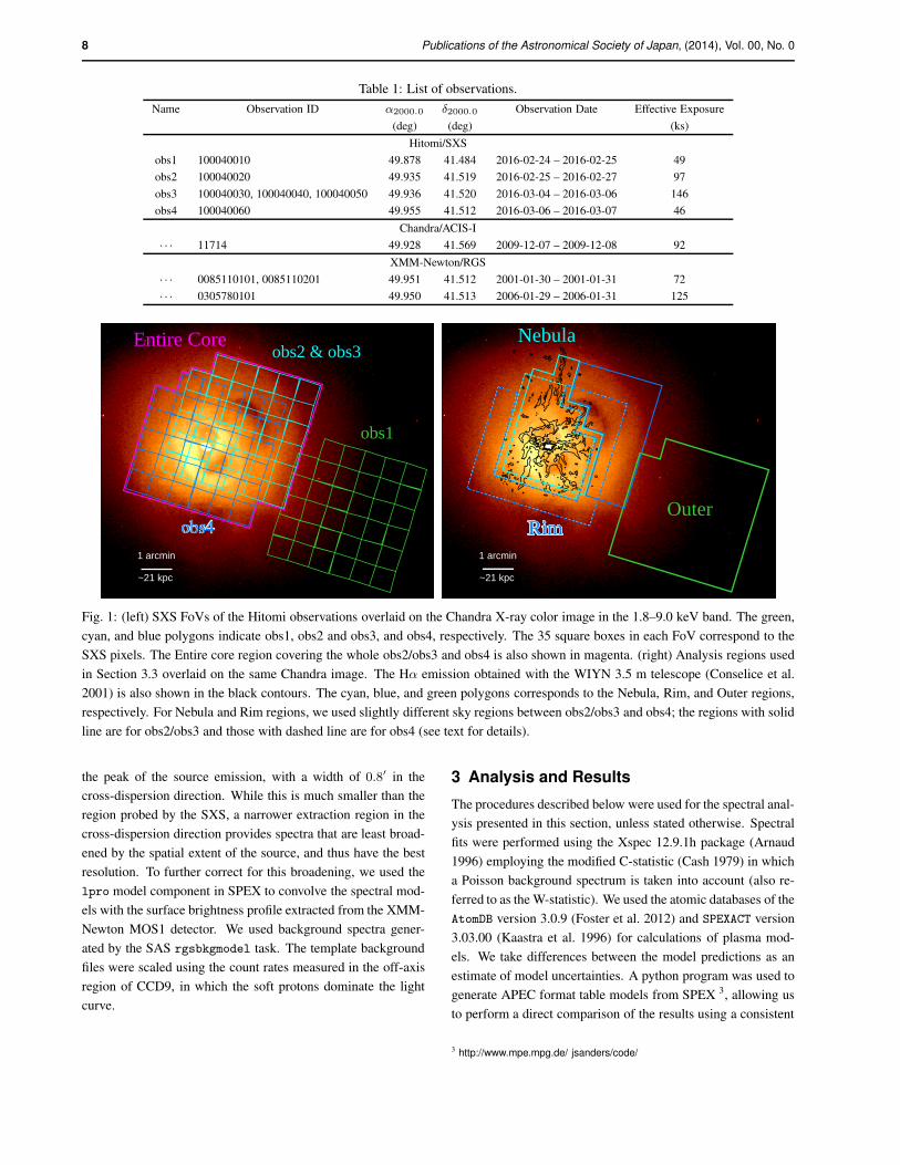
Table 1: List of observations.
Name Observation ID α2000.0 δ2000.0 Observation Date Effective Exposure
(deg) (deg) (ks)
Hitomi/SXS
obs1 100040010 49.878 41.484 2016-02-24 – 2016-02-25 49
obs2 100040020 49.935 41.519 2016-02-25 – 2016-02-27 97
obs3 100040030, 100040040, 100040050 49.936 41.520 2016-03-04 – 2016-03-06 146
obs4 100040060 49.955 41.512 2016-03-06 – 2016-03-07 46
Chandra/ACIS-I
· · · 11714 49.928 41.569 2009-12-07 – 2009-12-08 92
XMM-Newton/RGS
· · · 0085110101, 0085110201 49.951 41.512 2001-01-30 – 2001-01-31 72
· · · 0305780101 49.950 41.513 2006-01-29 – 2006-01-31 125
1 arcmin
~21 kpc
obs2 & obs3
obs1
Entire Core
obs4
1 arcmin
~21 kpc
Outer
Nebula
RimRim
Fig. 1: (left) SXS FoVs of the Hitomi observations overlaid on the Chandra X-ray color image in the 1.8–9.0 keV band. The green,
cyan, and blue polygons indicate obs1, obs2 and obs3, and obs4, respectively. The 35 square boxes in each FoV correspond to the
SXS pixels. The Entire core region covering the whole obs2/obs3 and obs4 is also shown in magenta. (right) Analysis regions used
in Section 3.3 overlaid on the same Chandra image. The Hα emission obtained with the WIYN 3.5 m telescope (Conselice et al.
2001) is also shown in the black contours. The cyan, blue, and green polygons corresponds to the Nebula, Rim, and Outer regions,
respectively. For Nebula and Rim regions, we used slightly different sky regions between obs2/obs3 and obs4; the regions with solid
line are for obs2/obs3 and those with dashed line are for obs4 (see text for details).
the peak of the source emission, with a width of 0.8′ in the
cross-dispersion direction. While this is much smaller than the
region probed by the SXS, a narrower extraction region in the
cross-dispersion direction provides spectra that are least broad-
ened by the spatial extent of the source, and thus have the best
resolution. To further correct for this broadening, we used the
lpro model component in SPEX to convolve the spectral mod-
els with the surface brightness profile extracted from the XMM-
Newton MOS1 detector. We used background spectra gener-
ated by the SAS rgsbkgmodel task. The template background
files were scaled using the count rates measured in the off-axis
region of CCD9, in which the soft protons dominate the light
curve.
3 Analysis and Results
The procedures described below were used for the spectral anal-
ysis presented in this section, unless stated otherwise. Spectral
fits were performed using the Xspec 12.9.1h package (Arnaud
1996) employing the modified C-statistic (Cash 1979) in which
a Poisson background spectrum is taken into account (also re-
ferred to as the W-statistic). We used the atomic databases of the
AtomDB version 3.0.9 (Foster et al. 2012) and SPEXACT version
3.03.00 (Kaastra et al. 1996) for calculations of plasma mod-
els. We take differences between the model predictions as an
estimate of model uncertainties. A python program was used to
generate APEC format table models from SPEX 3, allowing us
to perform a direct comparison of the results using a consistent
3 http://www.mpe.mpg.de/ jsanders/code/
Publications of the Astronomical Society of Japan, (2014), Vol. 00, No. 0 9
1 102 5 20
10−
30.
010.
11
Cou
nts
s−1
keV
−1
Energy (keV)
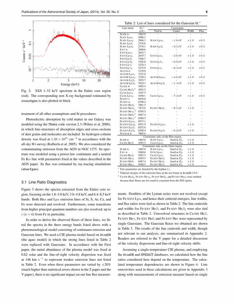
Fig. 2: SXS 1–32 keV spectrum in the Entire core region
(red). The corresponding non X-ray background estimated by
sxsnxbgen is also plotted in black.
treatment of all other assumptions and fit procedures.
Photoelectric absorption by cold matter in our Galaxy was
modeled using the TBabs code version 2.3 (Wilms et al. 2000),
in which fine-structures of absorption edges and cross-sections
of dust grains and molecules are included. Its hydrogen column
density was fixed at 1.38× 1021 cm−2 in accordance with the
all-sky H I survey (Kalberla et al. 2005). We also considered the
contaminating emission from the AGN in NGC 1275. Its spec-
trum was modeled using a power-law continuum and a neutral
Fe Kα line with parameters fixed at the values described in the
AGN paper. Its flux was estimated by ray-tracing simulations
(aharfgen).
3.1 Line Ratio Diagnostics
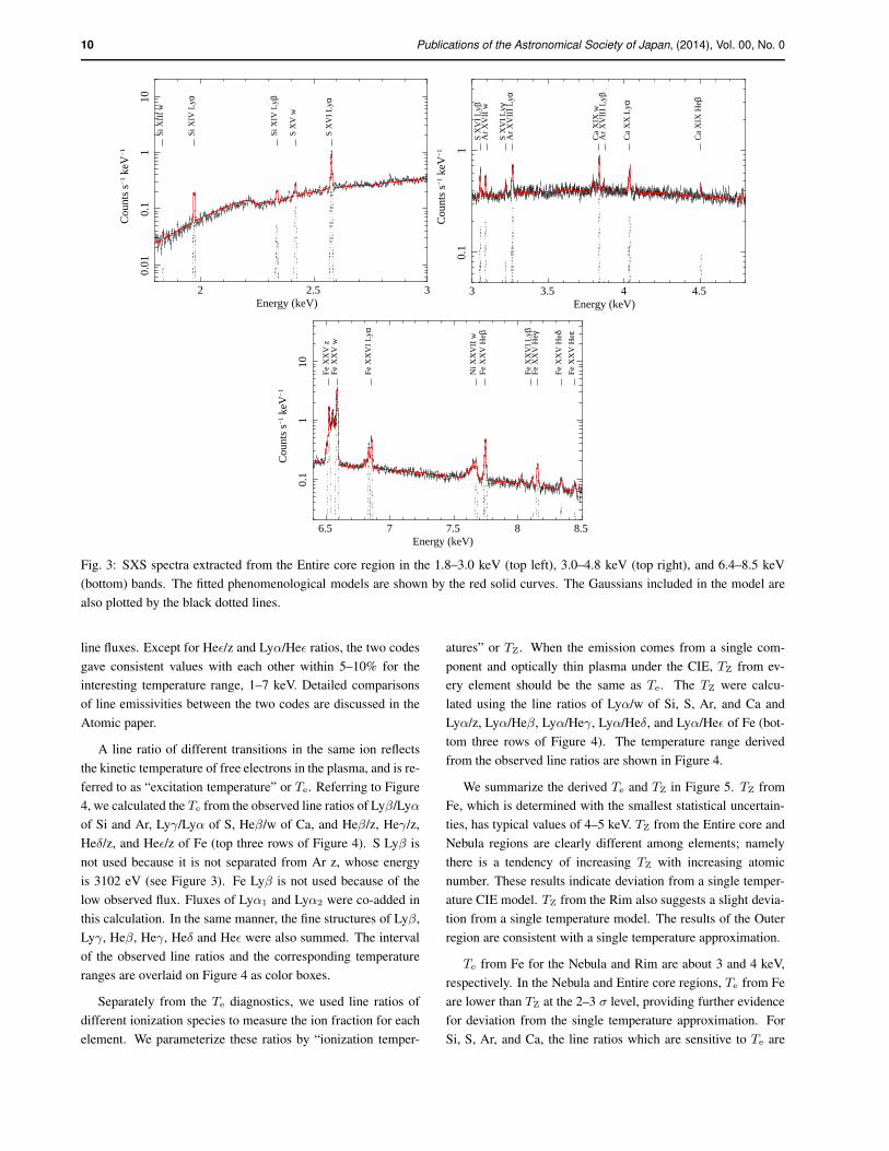
Figure 3 shows the spectra extracted from the Entire core re-
gion, focusing on the 1.8–3.0 keV, 3.0–4.8 keV, and 6.4–8.5 keV
bands. Both Heα and Lyα emission lines of Si, S, Ar, Ca, and
Fe were detected and resolved. Furthermore, some transitions
from higher principal quantum numbers are also resolved; up to
ǫ (n= 6) from Fe in particular.
In order to derive the observed fluxes of these lines, we fit-
ted the spectra in the three energy bands listed above with a
phenomenological model consisting of continuum emission and
Gaussian lines. We used a CIE plasma model based on AtomDB
(the apec model) in which the strong lines listed in Table 2
were replaced with Gaussians. In accordance with the First
paper, the metal abundance of the plasma model was fixed at
0.62 solar and the line-of-sight velocity dispersion was fixed
at 146 km s−1 to represent weaker emission lines not listed
in Table 2. Even when these parameters are varied by ±20%
(much higher than statistical errors shown in the Z paper and the
V paper), there is no significant impact on our line flux measure-
Table 2: List of lines considered for the Gaussian fit.∗
Line name E0† Constraints
(eV) Tied to Center Width Flux
Si XIII w 1865.0 - - - -
Si XIV Lyα1 2006.1 - - - -
Si XIV Lyα2 2004.3 Si XIV Lyα1 −1.8 eV ×1.0 ×0.5Si XIV Lyβ1 2376.6 - - - -
Si XIV Lyβ2 2376.1 Si XIV Lyβ1 −0.5 eV ×1.0 ×0.5S XV w 2460.6 - - - -
S XVI Lyα1 2622.7 - - - -
S XVI Lyα2 2619.7 S XVI Lyα1 −3.0 eV ×1.0 ×0.5S XVI Lyβ1 3106.7 - - - -
S XVI Lyβ2 3105.8 S XVI Lyβ1 −0.9 eV ×1.0 ×0.5S XVI Lyγ1 3276.3 - - - -
S XVI Lyγ2 3275.9 S XVI Lyγ1 −0.4 eV ×1.0 ×0.5Ar XVII w 3139.6 - - - -
Ar XVIII Lyα1 3323.0 - - - -
Ar XVIII Lyα2 3328.2 Ar XVIII Lyα1 −4.8 eV ×1.0 ×0.5Ar XVIII Lyβ1 3935.7 - - - -
Ar XVIII Lyβ2 3934.3 Ar XVIII Lyβ1 −1.4 eV ×1.0 ×0.5Ca XIX w 3902.4 - - - -
Ca XIX Heβ1‡ 4583.5 - - - -
Ca XX Lyα1 4107.5 - - - -
Ca XX Lyα2 4100.1 Ca XX Lyα1 −7.4 eV ×1.0 ×0.5Fe XXV z 6636.6 - - - -
Fe XXV w 6700.4 - - - -
Fe XXV Heβ1 7881.5 - - - -
Fe XXV Heβ2 7872.0 Fe XXV Heβ1 −9.5 eV ×1.0 -
Fe XXV Heγ1‡ 8295.5 - - - -
Fe XXV Heδ1‡ 8487.4 - - - -
Fe XXV Heǫ1‡ 8588.5 - - - -
Fe XXVI Lyα1 6973.1 - - - -
Fe XXVI Lyα2 6951.9 Fe XXVI Lyα1 - ×1.0 -
Fe XXVI Lyβ1 8252.6 - - - -
Fe XXVI Lyβ2 8248.4 Fe XXVI Lyβ1 −6.2 eV ×1.0 -
Ni XXVII w 7805.6 - - - -
Constraints only on the Rim region
Si XIII w 1865.0 Si XIV Lyα1 fixed at E0 ×1.0 -
Ca XIX Heβ1 4583.5 Ca XX Lyα1 fixed at E0 ×1.0 -
Constraints only on the Outer region
Si XIII w 1865.0 Si XIV Lyα1 fixed at E0 ×1.0 -
S XV w 2460.6 S XVI Lyα1 fixed at E0 ×1.0 -
Ca XIX Heβ1 4583.5 Ca XX Lyα1 fixed at E0 ×1.0 -
Fe XXV Heγ1 8295.5 Fe XXV Heβ1 fixed at E0 ×1.0 -
Fe XXV Heδ1 8487.4 Fe XXV Heβ1 fixed at E0 ×1.0 -
Fe XXV Heǫ1 8588.5 Fe XXV Heβ1 fixed at E0 ×1.0 -
∗ Free parameters are denoted by the hyphen (-).† Fiducial energies of the emission lines at the rest frame in AtomDB 3.0.9‡ Ca XIX Heβ2, Fe XXV Heγ2, Fe XXV Heδ2 , and Fe XXV Heǫ2 were omitted
because their fluxes are too small to constrain from the SXS spetra.
ments. Doublets of the Lyman series were not resolved except
for Fe XXVI Lyα, and hence their centroid energies, line widths,
and flux ratios were tied as shown in Table 2. The line centroids
and widths for Fe XXV Heβ1 and Fe XXV Heβ2 were also tied
as described in Table 2. Unresolved structures in Ca XIX Heβ,
Fe XXV Heγ, Fe XXV Heδ, and Fe XXV Heǫ were represented by
single Gaussians. The Gaussian fluxes we obtained are shown
in Table 3. The results of the line centroids and width, though
not relevant to our analysis, are summarized in Appendix 2.
Readers are referred to the V paper for a detailed discussion
of the velocity dispersions and line-of-sight velocity shifts.
Assuming a single-temperature CIE plasma, and employing
the AtomDB and SPEXACT databases, we calculated how the line
ratios considered here depend on the temperature. The calcu-
lated temperature dependencies are shown in Figure 4. Line
emissivities used in these calculations are given in Appendix 3
along with measurements of emission measure based on single
10 Publications of the Astronomical Society of Japan, (2014), Vol. 00, No. 0
2 2.5 3
0.01
0.1
110
Cou
nts
s−1
keV
−1
Energy (keV)
Si X
III w
Si X
IV L
yα
Si X
IV L
yβ
S X
V w
S X
VI L
yα
3 3.5 4 4.5
0.1
1
Cou
nts
s−1
keV
−1
Energy (keV)
S X
VI L
yβ
S X
VI L
yγ
Ar
XV
II w
Ar
XV
III L
yα
Ar
XV
III L
yβ
Ca
XIX
w
Ca
XX
Lyα
Ca
XIX
Heβ
6.5 7 7.5 8 8.5
0.1
110
Cou
nts
s−1
keV
−1
Energy (keV)
Fe
XX
V z
Fe
XX
V w
Fe
XX
VI L
yα
Fe
XX
V H
eβ
Fe
XX
VI L
yβ F
e X
XV
Heγ
Fe
XX
V H
eδ F
e X
XV
Heε
Ni X
XV
II w
Fig. 3: SXS spectra extracted from the Entire core region in the 1.8–3.0 keV (top left), 3.0–4.8 keV (top right), and 6.4–8.5 keV
(bottom) bands. The fitted phenomenological models are shown by the red solid curves. The Gaussians included in the model are
also plotted by the black dotted lines.
line fluxes. Except for Heǫ/z and Lyα/Heǫ ratios, the two codes
gave consistent values with each other within 5–10% for the
interesting temperature range, 1–7 keV. Detailed comparisons
of line emissivities between the two codes are discussed in the
Atomic paper.
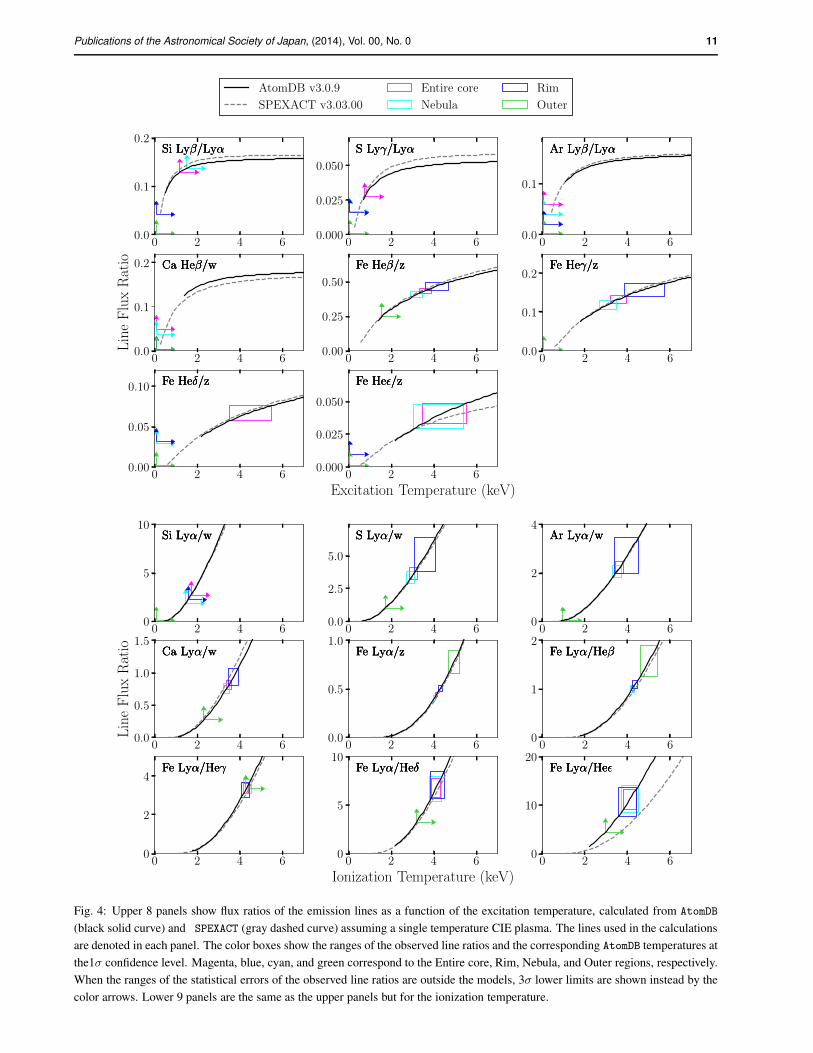
A line ratio of different transitions in the same ion reflects
the kinetic temperature of free electrons in the plasma, and is re-
ferred to as “excitation temperature” or Te. Referring to Figure
4, we calculated the Te from the observed line ratios of Lyβ/Lyα
of Si and Ar, Lyγ/Lyα of S, Heβ/w of Ca, and Heβ/z, Heγ/z,
Heδ/z, and Heǫ/z of Fe (top three rows of Figure 4). S Lyβ is
not used because it is not separated from Ar z, whose energy
is 3102 eV (see Figure 3). Fe Lyβ is not used because of the
low observed flux. Fluxes of Lyα1 and Lyα2 were co-added in
this calculation. In the same manner, the fine structures of Lyβ,
Lyγ, Heβ, Heγ, Heδ and Heǫ were also summed. The interval
of the observed line ratios and the corresponding temperature
ranges are overlaid on Figure 4 as color boxes.
Separately from the Te diagnostics, we used line ratios of
different ionization species to measure the ion fraction for each
element. We parameterize these ratios by “ionization temper-
atures” or TZ. When the emission comes from a single com-
ponent and optically thin plasma under the CIE, TZ from ev-
ery element should be the same as Te. The TZ were calcu-
lated using the line ratios of Lyα/w of Si, S, Ar, and Ca and
Lyα/z, Lyα/Heβ, Lyα/Heγ, Lyα/Heδ, and Lyα/Heǫ of Fe (bot-
tom three rows of Figure 4). The temperature range derived
from the observed line ratios are shown in Figure 4.
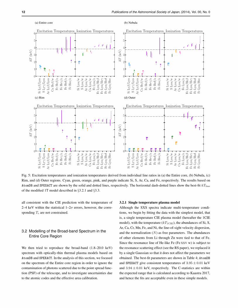
We summarize the derived Te and TZ in Figure 5. TZ from
Fe, which is determined with the smallest statistical uncertain-
ties, has typical values of 4–5 keV. TZ from the Entire core and
Nebula regions are clearly different among elements; namely
there is a tendency of increasing TZ with increasing atomic
number. These results indicate deviation from a single temper-
ature CIE model. TZ from the Rim also suggests a slight devia-
tion from a single temperature model. The results of the Outer
region are consistent with a single temperature approximation.
Te from Fe for the Nebula and Rim are about 3 and 4 keV,
respectively. In the Nebula and Entire core regions, Te from Fe
are lower than TZ at the 2–3 σ level, providing further evidence
for deviation from the single temperature approximation. For
Si, S, Ar, and Ca, the line ratios which are sensitive to Te are
Publications of the Astronomical Society of Japan, (2014), Vol. 00, No. 0 11
0 2 4 60.0
0.1
0.2Si Lyβ/LyαSi Lyβ/LyαSi Lyβ/LyαSi Lyβ/Lyα
0 2 4 60.000
0.025
0.050
S Lyγ/LyαS Lyγ/LyαS Lyγ/LyαS Lyγ/Lyα
0 2 4 60.0
0.1
Ar Lyβ/LyαAr Lyβ/LyαAr Lyβ/LyαAr Lyβ/Lyα
0 2 4 60.0
0.1
0.2
LineFluxRatio Ca Heβ/wCa Heβ/wCa Heβ/wCa Heβ/w
0 2 4 60.00
0.25
0.50
Fe Heβ/zFe Heβ/zFe Heβ/zFe Heβ/z
0 2 4 60.0
0.1
0.2Fe Heγ/zFe Heγ/zFe Heγ/zFe Heγ/z
0 2 4 60.00
0.05
0.10 Fe Heδ/zFe Heδ/zFe Heδ/zFe Heδ/z
0 2 4 6
Excitation Temperature (keV)
0.000
0.025
0.050
Fe Heǫ/zFe Heǫ/zFe Heǫ/zFe Heǫ/z
0 2 4 60
5
10Si Lyα/wSi Lyα/wSi Lyα/wSi Lyα/w
0 2 4 60.0
2.5
5.0
S Lyα/wS Lyα/wS Lyα/wS Lyα/w
0 2 4 60
2
4Ar Lyα/wAr Lyα/wAr Lyα/wAr Lyα/w
0 2 4 60.0
0.5
1.0
1.5
LineFluxRatio Ca Lyα/wCa Lyα/wCa Lyα/wCa Lyα/w
0 2 4 60.0
0.5
1.0Fe Lyα/zFe Lyα/zFe Lyα/zFe Lyα/z
0 2 4 60
1
2Fe Lyα/HeβFe Lyα/HeβFe Lyα/HeβFe Lyα/Heβ
0 2 4 60
2
4Fe Lyα/HeγFe Lyα/HeγFe Lyα/HeγFe Lyα/Heγ
0 2 4 6
Ionization Temperature (keV)
0
5
10Fe Lyα/HeδFe Lyα/HeδFe Lyα/HeδFe Lyα/Heδ
0 2 4 60
10
20Fe Lyα/HeǫFe Lyα/HeǫFe Lyα/HeǫFe Lyα/Heǫ
AtomDB v3.0.9
SPEXACT v3.03.00
Entire core
Nebula
Rim
Outer
Fig. 4: Upper 8 panels show flux ratios of the emission lines as a function of the excitation temperature, calculated from AtomDB
(black solid curve) and SPEXACT (gray dashed curve) assuming a single temperature CIE plasma. The lines used in the calculations
are denoted in each panel. The color boxes show the ranges of the observed line ratios and the corresponding AtomDB temperatures at
the1σ confidence level. Magenta, blue, cyan, and green correspond to the Entire core, Rim, Nebula, and Outer regions, respectively.
When the ranges of the statistical errors of the observed line ratios are outside the models, 3σ lower limits are shown instead by the
color arrows. Lower 9 panels are the same as the upper panels but for the ionization temperature.
12 Publications of the Astronomical Society of Japan, (2014), Vol. 00, No. 0
(a) Entire core
SiLyβ
/Lyα
SLyγ
/Lyα
ArLyβ
/Lyα
CaHeβ
/w
FeHeβ
/z
FeHeγ/z
FeHeδ/z
FeHeǫ/z
0
1
2
3
4
5
6kT
(keV
)Excitation Temperatures
SiLyα
/w
SLyα
/w
ArLyα
/w
CaLyα
/w
FeLyα
/z
FeLyα
/Heβ
FeLyα
/Heγ
FeLyα
/Heδ
FeLyα
/Heǫ
Ionization Temperatures
(b) Nebula
SiLyβ
/Lyα
SLyγ
/Lyα
ArLyβ
/Lyα
CaHeβ
/w
FeHeβ
/z
FeHeγ/z
FeHeδ/z
FeHeǫ/z
0
1
2
3
4
5
6
kT
(keV
)
Excitation Temperatures
SiLyα
/w
SLyα
/w
ArLyα
/w
CaLyα
/w
FeLyα
/z
FeLyα
/Heβ
FeLyα
/Heγ
FeLyα
/Heδ
FeLyα
/Heǫ
Ionization Temperatures
(c) Rim
SiLyβ
/Lyα
SLyγ
/Lyα
ArLyβ
/Lyα
CaHeβ
/w
FeHeβ
/z
FeHeγ/z
FeHeδ/z
FeHeǫ/z
0
1
2
3
4
5
6
kT
(keV
)
Excitation Temperatures
SiLyα
/w
SLyα
/w
ArLyα
/w
CaLyα
/w
FeLyα
/z
FeLyα
/Heβ
FeLyα
/Heγ
FeLyα
/Heδ
FeLyα
/Heǫ
Ionization Temperatures
(d) Outer
SiLyβ
/Lyα
SLyγ
/Lyα
ArLyβ
/Lyα
CaHeβ
/w
FeHeβ
/z
FeHeγ/z
FeHeδ/z
FeHeǫ/z
0
1
2
3
4
5
6
kT
(keV
)
Excitation Temperatures
SiLyα
/w
SLyα
/w
ArLyα
/w
CaLyα
/w
FeLyα
/z
FeLyα
/Heβ
FeLyα
/Heγ
FeLyα
/Heδ
FeLyα
/Heǫ
Ionization Temperatures
Fig. 5: Excitation temperatures and ionization temperatures derived from individual line ratios in (a) the Entire core, (b) Nebula, (c)
Rim, and (d) Outer regions. Cyan, green, orange, pink, and purple indicate Si, S, Ar, Ca, and Fe, respectively. The results based on
AtomDB and SPEXACT are shown by the solid and dotted lines, respectively. The horizontal dash-dotted lines show the best-fit kTline
of the modified 1T model described in §3.2.1 and §3.3.
all consistent with the CIE prediction with the temperature of
2–4 keV within the statistical 1–2σ errors, however, the corre-
sponding Te are not constrained.
3.2 Modelling of the Broad-band Spectrum in the
Entire Core Region
We then tried to reproduce the broad-band (1.8–20.0 keV)
spectrum with optically-thin thermal plasma models based on
AtomDB and SPEXACT. In the analysis of this section, we focused
on the spectrum of the Entire core region in order to ignore the
contamination of photons scattered due to the point spread func-
tion (PSF) of the telescope, and to investigate uncertainties due
to the atomic codes and the effective area calibration.
3.2.1 Single temperature plasma model
Although the SXS spectra indicate multi-temperature condi-
tions, we begin by fitting the data with the simplest model, that
is, a single temperature CIE plasma model (hereafter the 1CIE
model), with the temperature (kT1CIE), the abundances of Si, S,
Ar, Ca, Cr, Mn, Fe, and Ni, the line-of-sight velocity dispersion,
and the normalization (N) as free parameters. The abundances
of other elements from Li through Zn were tied to that of Fe.
Since the resonance line of He-like Fe (Fe XXV w) is subject to
the resonance scattering effect (see the RS paper), we replaced it
by a single Gaussian so that it does not affect the parameters we
obtained. The best-fit parameters are shown in Table 4; AtomDB
and SPEXACT give consistent temperatures of 3.95± 0.01 keV
and 3.94± 0.01 keV, respectively. The C-statistics are within
the expected range that is calculated according to Kaastra 2017,
and hence the fits are acceptable even in these simple models.
Publications of the Astronomical Society of Japan, (2014), Vol. 00, No. 0 13
(a)
102 5 20
10−4
10−3
0.01
0.1
1
Cou
nts
s−1
keV
−1
Energy (keV)
(b)
0.1
0.2
0.3
0.4
Cou
nts
s−1
keV
−1
0.81
1.2
Mod
elD
ata
/
0.91
1.1
Ato
mD
BS
PE
XA
CT
/
1.8 2 2.2 2.4
0.91
1.1
1CIE
2CIE
/
Energy (keV)
(c)
0.5
1
Cou
nts
s−1
keV
−1
0.81
1.2
Mod
elD
ata
/
0.91
1.1
Ato
mD
BS
PE
XA
CT
/
2.6 2.8 3 3.2 3.4
0.91
1.1
1CIE
2CIE
/
Energy (keV)
(d)
0.20.40.60.8
1
Cou
nts
s−1
keV
−1
0.81
1.2M
odel
Dat
a /
0.91
1.1
Ato
mD
BS
PE
XA
CT
/
3.8 4 4.2 4.4 4.6
0.91
1.1
1CIE
2CIE
/
Energy (keV)
(e)
1
2
3
4
Cou
nts
s−1
keV
−1
0.81
1.2
Mod
elD
ata
/
0.91
1.1
Ato
mD
BS
PE
XA
CT
/
6.5 6.6 6.7 6.8 6.9
0.91
1.1
1CIE
2CIE
/
Energy (keV)
(f)
0.10.20.30.40.5
Cou
nts
s−1
keV
−1
0.81
1.2
Mod
elD
ata
/
0.91
1.1
Ato
mD
BS
PE
XA
CT
/
7.6 7.8 8 8.2 8.4
0.91
1.1
1CIE
2CIE
/
Energy (keV)
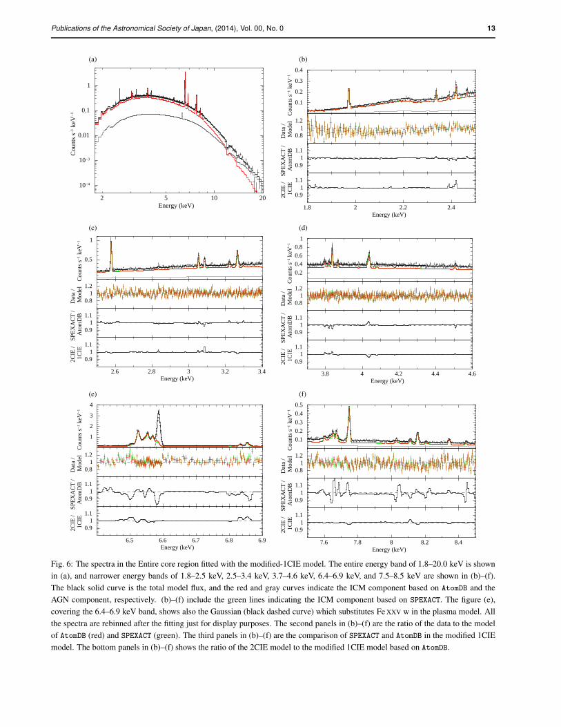
Fig. 6: The spectra in the Entire core region fitted with the modified-1CIE model. The entire energy band of 1.8–20.0 keV is shown
in (a), and narrower energy bands of 1.8–2.5 keV, 2.5–3.4 keV, 3.7–4.6 keV, 6.4–6.9 keV, and 7.5–8.5 keV are shown in (b)–(f).
The black solid curve is the total model flux, and the red and gray curves indicate the ICM component based on AtomDB and the
AGN component, respectively. (b)–(f) include the green lines indicating the ICM component based on SPEXACT. The figure (e),
covering the 6.4–6.9 keV band, shows also the Gaussian (black dashed curve) which substitutes Fe XXV w in the plasma model. All
the spectra are rebinned after the fitting just for display purposes. The second panels in (b)–(f) are the ratio of the data to the model
of AtomDB (red) and SPEXACT (green). The third panels in (b)–(f) are the comparison of SPEXACT and AtomDB in the modified 1CIE
model. The bottom panels in (b)–(f) shows the ratio of the 2CIE model to the modified 1CIE model based on AtomDB.
14 Publications of the Astronomical Society of Japan, (2014), Vol. 00, No. 0
Table 3: Observed line fluxes derived from Gaussian fits.∗
Line name Flux (10−5 ph cm−2 s−1)
Entire Core Nebula Rim Outer
Si XIII w 6.40+4.71
−2.675.87
+3.60
−2.54<5.45 <4.54
Si XIV Lyα1 32.43+2.29
−2.2320.11
+1.92
−1.8321.83
+2.64
−2.524.09
+2.27
−1.72
Si XIV Lyβ1 6.96+0.91
−0.875.03
+0.74
−0.703.93
+1.04
−0.981.21
+0.82
−0.58
S XV w 9.38+1.13
−1.117.26
+0.98
−0.993.91
+1.03
−0.94<1.08
S XVI Lyα1 22.71+0.73
−0.7215.81
+0.64
−0.6312.46
+0.77
−0.762.70
+0.67
−0.64
S XVI Lyβ1 3.83+0.29
−0.292.55+0.25
−0.242.49+0.35
−0.330.62+0.27
−0.22
S XVI Lyγ1 1.20+0.20
−0.190.74
+0.15
−0.170.92
+0.25
−0.240.32
+0.22
−0.17
Ar XVII w 3.72+0.37
−0.362.82
+0.31
−0.301.87
+0.51
−0.471.20
+0.41
−0.34
Ar XVIII Lyα1 5.47+0.29
−0.293.85
+0.25
−0.253.15
+0.32
−0.300.94
+0.32
−0.30
Ar XVIII Lyβ1 0.77+0.15
−0.150.51
+0.12
−0.120.63
+0.20
−0.180.26
+0.15
−0.11
Ca XIX w 5.20+0.27
−0.273.66
+0.23
−0.232.94
+0.30
−0.280.93
+0.29
−0.26
Ca XIX Heβ1 0.66+0.16
−0.100.46
+0.13
−0.100.67
+0.29
−0.350.21
+0.16
−0.12
Ca XX Lyα1 2.80+0.18
−0.181.85
+0.16
−0.151.81
+0.20
−0.190.77
+0.20
−0.19
Fe XXV w 33.14+0.43
−0.3421.09
+0.32
−0.3122.13
+0.49
−0.359.49
+0.45
−0.44
Fe XXV z 13.26+0.27
−0.258.72
+0.21
−0.228.41
+0.28
−0.273.03
+0.28
−0.27
Fe XXV Heβ1 4.73+0.12
−0.242.80
+0.12
−0.153.35
+0.19
−0.181.49
+0.21
−0.20
Fe XXV Heβ2 1.04+0.10
−0.180.73
+0.14
−0.080.55
+0.13
−0.13<0.17
Fe XXV Heγ1 1.75+0.13
−0.131.04
+0.10
−0.101.32
+0.14
−0.130.25
+0.13
−0.12
Fe XXV Heδ1 0.88+0.12
−0.120.55
+0.10
−0.100.63
+0.13
−0.120.27
+0.13
−0.11
Fe XXV Heǫ1 0.54+0.10
−0.100.34
+0.08
−0.080.43
+0.12
−0.120.15
+0.12
−0.10
Fe XXVI Lyα1 3.68+0.16
−0.162.24+0.13
−0.132.68+0.17
−0.171.35+0.22
−0.21
Fe XXVI Lyα2 2.17+0.14
−0.131.31
+0.12
−0.111.59
+0.14
−0.140.99
+0.20
−0.18
Fe XXVI Lyβ1 0.30+0.06
−0.060.21
+0.06
−0.050.18
+0.07
−0.040.16
+0.08
−0.06
Ni XXVII w 1.43+0.13
−0.131.01
+0.11
−0.110.79
+0.13
−0.130.43
+0.16
−0.15
∗ The Lyα2 lines of Si, S, Ar, and Ca are not shown because their parameter values
are tied to Lyα1 (see Table 2 for details).
Table 4: Best fit parameters for the Entire core region
Model/Parameter AtomDB v3.0.9 SPEXACT v3.03.00
1CIE model
kT1CIE (keV) 3.95+0.01−0.01 3.94+0.01
−0.01
N (1012 cm−5) 23.20+0.05−0.05
22.78+0.04−0.04
C-statistics/dof 13123.6/12979 13181.7/12979
Modified 1CIE model
kTcont (keV) 4.01+0.01−0.01 3.95+0.01
−0.01
kTline (keV) 3.80+0.02−0.02
3.89+0.02−0.02
N (1012 cm−5) 22.77+0.04−0.04
22.67+0.05−0.05
C-statistics/dof 13085.9/12978 13178.7/12978
2CIE model (modified CIE + CIE)
kTcont1 (keV) 3.66+0.01−0.02 3.40+0.02
−0.01
kTline1 (keV) 3.06+0.04−0.03
2.92+0.03−0.03
kT2 (keV) 4.51+0.02−0.03
4.73+0.02−0.02
N1 (1012 cm−5) 12.98+0.05−0.05 13.27+0.13
−0.09
N2 (1012 cm−5) 9.71+0.06−0.05 9.45+0.07
−0.05
C-statistics/dof 13058.5/12976 13093.9/12976
Power-law DEM model
index 10.92+0.11−0.11
4.68+0.03−0.03
kTmax (keV) 4.01+0.06−0.01 4.29+0.01
−0.01
N (1012 cm−5) 21.38+0.24−0.24 15.39+0.04
−0.04
C-statistics/dof 13123.4/12978 13147.6/12978
Gaussian DEM model
kTmean (keV) 3.94+0.01−0.01
3.89+0.01−0.01
σ (keV) 0.60+0.08−0.11 1.01+0.05
−0.05
N (1012 cm−5) 11.65+0.02−0.02 11.67+0.03
−0.03
C-statistics/dof 13121.1/12978 13138.7/12978
3.8
4.0
4.2
kT
(keV
)
kTcont1
kTline1
ARFnormal ARFground ARFCrab ARFnormal ARFground ARFCrab
12900
13000
13100
13200
13300
C-statistics
——– AtomDB 3.0.9 ——– —— SPEXACT 3.03.00 ——
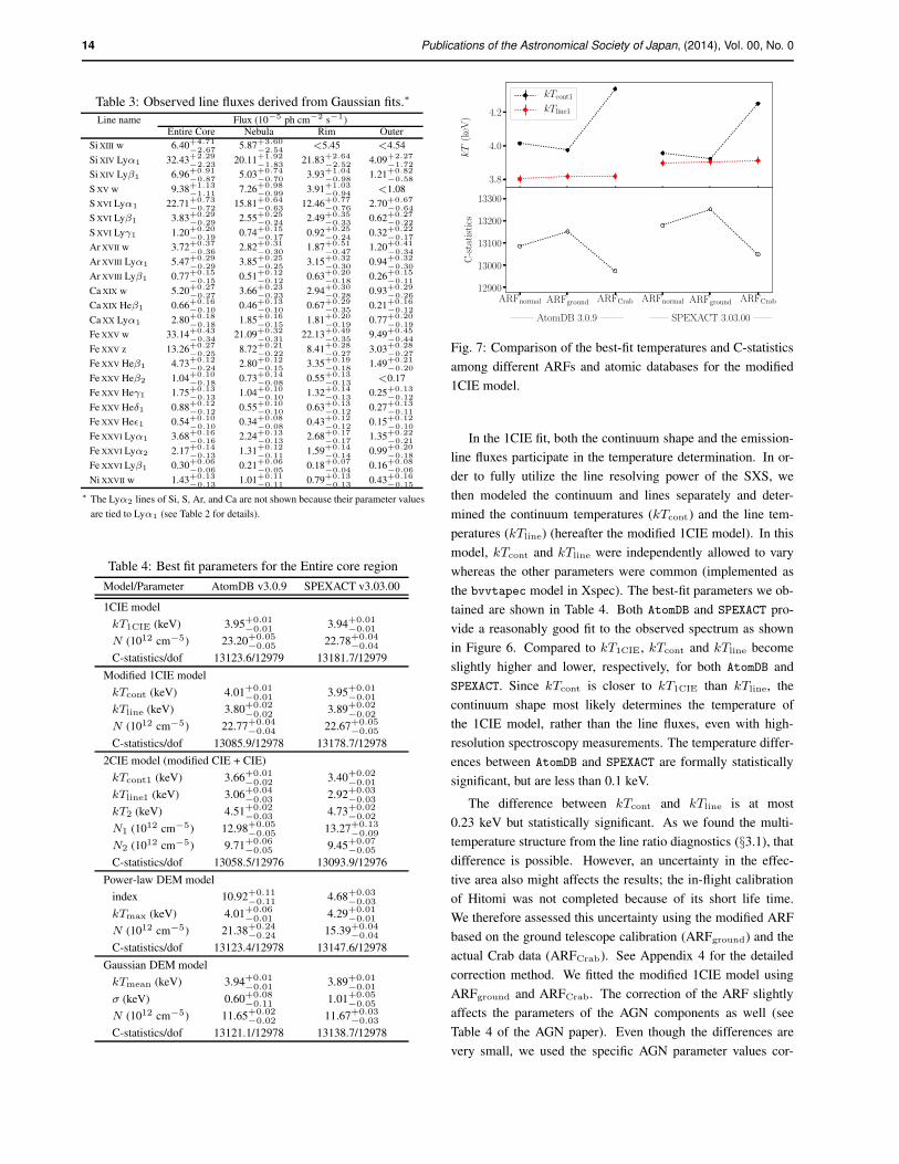
Fig. 7: Comparison of the best-fit temperatures and C-statistics
among different ARFs and atomic databases for the modified
1CIE model.
In the 1CIE fit, both the continuum shape and the emission-
line fluxes participate in the temperature determination. In or-
der to fully utilize the line resolving power of the SXS, we
then modeled the continuum and lines separately and deter-
mined the continuum temperatures (kTcont) and the line tem-
peratures (kTline) (hereafter the modified 1CIE model). In this
model, kTcont and kTline were independently allowed to vary
whereas the other parameters were common (implemented as
the bvvtapec model in Xspec). The best-fit parameters we ob-
tained are shown in Table 4. Both AtomDB and SPEXACT pro-
vide a reasonably good fit to the observed spectrum as shown
in Figure 6. Compared to kT1CIE, kTcont and kTline become
slightly higher and lower, respectively, for both AtomDB and
SPEXACT. Since kTcont is closer to kT1CIE than kTline, the
continuum shape most likely determines the temperature of
the 1CIE model, rather than the line fluxes, even with high-
resolution spectroscopy measurements. The temperature differ-
ences between AtomDB and SPEXACT are formally statistically
significant, but are less than 0.1 keV.
The difference between kTcont and kTline is at most
0.23 keV but statistically significant. As we found the multi-
temperature structure from the line ratio diagnostics (§3.1), that
difference is possible. However, an uncertainty in the effec-
tive area also might affects the results; the in-flight calibration
of Hitomi was not completed because of its short life time.
We therefore assessed this uncertainty using the modified ARF
based on the ground telescope calibration (ARFground) and the
actual Crab data (ARFCrab). See Appendix 4 for the detailed
correction method. We fitted the modified 1CIE model using
ARFground and ARFCrab. The correction of the ARF slightly
affects the parameters of the AGN components as well (see
Table 4 of the AGN paper). Even though the differences are
very small, we used the specific AGN parameter values cor-
Publications of the Astronomical Society of Japan, (2014), Vol. 00, No. 0 15
2
5
10
20kT
(keV
)kTcont1
kTline1
kT2
0.0
0.2
0.4
0.6
0.8
N2/N
1
ARFnormal ARFground ARFCrab ARFnormal ARFground ARFCrab
12900
13000
13100
13200
13300
C-statistics
——– AtomDB 3.0.9 ——– —— SPEXACT 3.03.00 ——
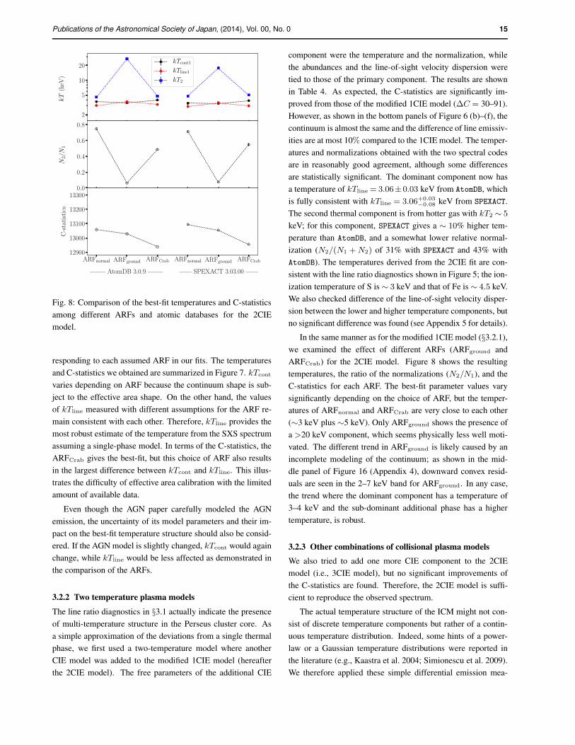
Fig. 8: Comparison of the best-fit temperatures and C-statistics
among different ARFs and atomic databases for the 2CIE
model.
responding to each assumed ARF in our fits. The temperatures
and C-statistics we obtained are summarized in Figure 7. kTcont
varies depending on ARF because the continuum shape is sub-
ject to the effective area shape. On the other hand, the values
of kTline measured with different assumptions for the ARF re-
main consistent with each other. Therefore, kTline provides the
most robust estimate of the temperature from the SXS spectrum
assuming a single-phase model. In terms of the C-statistics, the
ARFCrab gives the best-fit, but this choice of ARF also results
in the largest difference between kTcont and kTline. This illus-
trates the difficulty of effective area calibration with the limited
amount of available data.
Even though the AGN paper carefully modeled the AGN
emission, the uncertainty of its model parameters and their im-
pact on the best-fit temperature structure should also be consid-
ered. If the AGN model is slightly changed, kTcont would again
change, while kTline would be less affected as demonstrated in
the comparison of the ARFs.
3.2.2 Two temperature plasma models
The line ratio diagnostics in §3.1 actually indicate the presence
of multi-temperature structure in the Perseus cluster core. As
a simple approximation of the deviations from a single thermal
phase, we first used a two-temperature model where another
CIE model was added to the modified 1CIE model (hereafter
the 2CIE model). The free parameters of the additional CIE
component were the temperature and the normalization, while
the abundances and the line-of-sight velocity dispersion were
tied to those of the primary component. The results are shown
in Table 4. As expected, the C-statistics are significantly im-
proved from those of the modified 1CIE model (∆C = 30–91).
However, as shown in the bottom panels of Figure 6 (b)–(f), the
continuum is almost the same and the difference of line emissiv-
ities are at most 10% compared to the 1CIE model. The temper-
atures and normalizations obtained with the two spectral codes
are in reasonably good agreement, although some differences
are statistically significant. The dominant component now has
a temperature of kTline = 3.06±0.03 keV from AtomDB, which
is fully consistent with kTline = 3.06+0.03−0.08 keV from SPEXACT.
The second thermal component is from hotter gas with kT2 ∼ 5
keV; for this component, SPEXACT gives a ∼ 10% higher tem-
perature than AtomDB, and a somewhat lower relative normal-
ization (N2/(N1 +N2) of 31% with SPEXACT and 43% with
AtomDB). The temperatures derived from the 2CIE fit are con-
sistent with the line ratio diagnostics shown in Figure 5; the ion-
ization temperature of S is ∼ 3 keV and that of Fe is ∼ 4.5 keV.
We also checked difference of the line-of-sight velocity disper-
sion between the lower and higher temperature components, but
no significant difference was found (see Appendix 5 for details).
In the same manner as for the modified 1CIE model (§3.2.1),
we examined the effect of different ARFs (ARFground and
ARFCrab) for the 2CIE model. Figure 8 shows the resulting
temperatures, the ratio of the normalizations (N2/N1), and the
C-statistics for each ARF. The best-fit parameter values vary
significantly depending on the choice of ARF, but the temper-
atures of ARFnormal and ARFCrab are very close to each other
(∼3 keV plus ∼5 keV). Only ARFground shows the presence of
a >20 keV component, which seems physically less well moti-
vated. The different trend in ARFground is likely caused by an
incomplete modeling of the continuum; as shown in the mid-
dle panel of Figure 16 (Appendix 4), downward convex resid-
uals are seen in the 2–7 keV band for ARFground. In any case,
the trend where the dominant component has a temperature of
3–4 keV and the sub-dominant additional phase has a higher
temperature, is robust.
3.2.3 Other combinations of collisional plasma models
We also tried to add one more CIE component to the 2CIE
model (i.e., 3CIE model), but no significant improvements of
the C-statistics are found. Therefore, the 2CIE model is suffi-
cient to reproduce the observed spectrum.
The actual temperature structure of the ICM might not con-
sist of discrete temperature components but rather of a contin-
uous temperature distribution. Indeed, some hints of a power-
law or a Gaussian temperature distributions were reported in
the literature (e.g., Kaastra et al. 2004; Simionescu et al. 2009).
We therefore applied these simple differential emission mea-
16 Publications of the Astronomical Society of Japan, (2014), Vol. 00, No. 0
sure (DEM) models to the SXS spectrum. The emission mea-
sure profile, EM(kT ), is proportional to (kT/kTmax)α for
the power-law DEM model and to exp(−(kT − kTmean)2/2σ)
for the Gaussian DEM model. The best-fit parameters of the
models are summarized in Table 4. Both the power-law and
the Gaussian DEM models show steep temperature distribu-
tions peaked at ∼ 4 keV, even though the distributions based
on SPEXACT are slightly wider (smaller index or larger σ) than
those based on AtomDB. In any case, we found no significant im-
provements from the 2CIE model. Further investigation of the
multi-temperature model is shown in Section 3.4 and Figure 10.
Another possible cause of the deviation from a single tem-
perature model shown in the line ratio diagnostics is the NEI
state, which is often observed in supernova remnants. We
thus tried to fit the spectrum with a NEI model (the possibil-
ities of both an ionizing and a recombining plasma are con-
sidered). However, the obtained ionization parameter becomes
nt>1×1012 cm−3 s−1, and the temperature is almost the same
as the 1T model; therefore the model is consistent with a CIE
state, and we find no significant signature of the NEI.
3.3 Spatial Variation of the Temperature Structure
We next modeled the broad-band spectra in the Nebula, Rim,
and Outer regions in order to look for spatial trends in the tem-
perature distribution. The fit results obtained with the modified
1CIE model are shown in the top rows of Table 5. Compared
to the result from the Entire core region, the temperature in the
Nebula region is slightly lower, while that in the Rim region is
slightly higher. The temperature continues to increase at larger
radii, reaching 5 keV in the Outer region. These results are con-
sistent with the temperature map obtained from XMM-Newton
and Chandra observations (Churazov et al. 2003; Sanders &
Fabian 2007).
The line ratio diagnostics show a deviation from the single
temperature approximation in the Nebula and Rim regions. We
thus applied the 2CIE model to the spectra of those regions.
The best-fit parameters are also shown in the middle rows of
Table 5. The C-statistics were improved from the modified
1CIE model (∆C = 6–59). Both the Nebula and Rim regions
show the same composition as the Entire core (roughly 3 keV
plus 5 keV), but with different normalization ratios (the relative
contribution of the hotter component is lower in the Rim re-
gion, although significant differences between the two spectral
codes are also found). Large asymmetrical errors of the nor-
malizations in the Nebula region are likely due to the compara-
ble normalization values of the two components and the limited
energy band (> 1.8 keV). In the Nebula region, the discrep-
ancy between kTcont and kTline becomes large (∼1.0 keV), and
kTline shows the lowest temperature of ∼2.7 keV among the
different spatial regions considered. We also checked the 2CIE
model in the Outer region, but no improvements from the mod-
ified 1CIE model were found (∆C < 1), as expected from the
line ratio diagnostics. The systematic uncertainty of the tem-
perature measurements due to the different ARFs has a similar
trend as the analysis of the Entire core region (see Appendix 4).
The sizes of the regions used for spatially resolved spec-
troscopy are comparable to the angular resolution of the tele-
scope. Therefore, photons scattered from the adjacent regions
due to the telescope’s PSF tail might affect the fitting results.
We calculated the expected fraction of scattered photons with
ray-tracing simulations, and show the results in Table 6; the
fractions reach up to 30%, and are not negligible. We thus per-
formed a “PSF corrected” analysis, in which all the regions
were simultaneously fitted taking into account the expected
fluxes of photons scattered between regions. We used the 2CIE
model for the Nebula and Rim regions and the 1 CIE model for
the Outer region according to the results presented above. The
best-fit parameters of the PSF corrected model are shown in the
bottom rows of Table 5. After the PSF correction, the ratios
of the normalizations are changed but the temperatures we ob-
tained are almost consistent with those derived from the PSF
“uncorrected” analysis.
3.4 Comparison with Multi-temperature Models from
Previous Observations
Chandra/ACIS and XMM-Newton/RGS observations revealed
a multi-temperature structure ranging between 0.5–8.0 keV in
the core of the Perseus cluster (Sanders & Fabian 2007; Pinto
et al. 2016). Here we use a similar multi-temperature analysis to
check the consistency between Hitomi/SXS and these previous
measurements.
We fitted the SXS spectra extracted from the Nebula and
Rim regions with a six-temperature CIE model consisting of
0.5 keV, 1 keV, 2 keV, 3 keV, 4 keV and 8 keV components fol-
lowing Sanders & Fabian (2007). The temperature of each com-
ponent was fixed, and the abundance and line-of-sight velocity
dispersion were common to all the components. The power-
law component that was found in Sanders & Fabian (2007) and
interpreted as a possible inverse-Compton emission was also in-
cluded in our model with a fixed photon index of Γ = 2. The
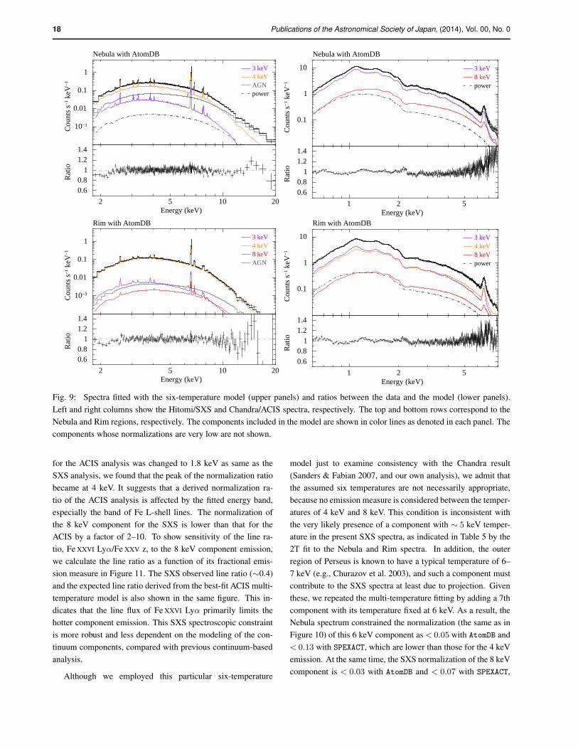
spectra and the best-fit models in the Nebula and the Rim re-
gions are shown in the left column of Figure 9. The normaliza-
tions we obtained for each temperature were scaled to sum to
unity, and the results are plotted in Figure 10 as red diamonds.
The profile of the scaled normalizations are very similar be-
tween AtomDB and SPEXACT, except for the 8 keV component
which is detected with SPEXACT in both the Nebula and Rim re-
gions while only its upper limit was obtained for AtomDB. The
results indicate that the combination of the 3 keV, 4 keV, and
8 keV components approximates the 2CIE model obtained in
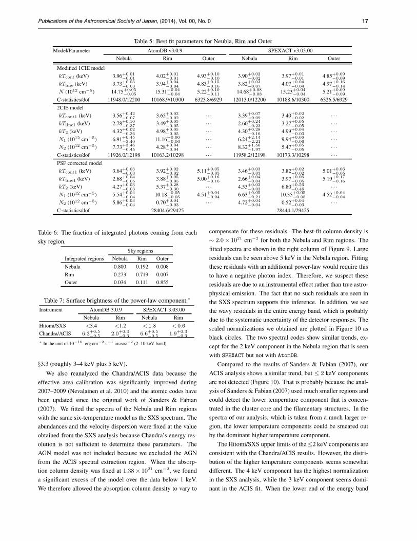
Publications of the Astronomical Society of Japan, (2014), Vol. 00, No. 0 17
Table 5: Best fit parameters for Neubla, Rim and Outer
Model/Parameter AtomDB v3.0.9 SPEXACT v3.03.00
Nebula Rim Outer Nebula Rim Outer
Modified 1CIE model
kTcont (keV) 3.96+0.01−0.01 4.02+0.01
−0.01 4.93+0.10−0.10 3.90+0.02
−0.02 3.97+0.01−0.01 4.85+0.09
−0.09
kTline (keV) 3.73+0.03−0.03
3.94+0.04−0.04
4.83+0.15−0.16
3.82+0.03−0.07
4.07+0.04−0.04
4.97+0.16−0.14
N (1012 cm−5) 14.75+0.05−0.05
15.31+0.04−0.04
5.22+0.10−0.11
14.68+0.08−0.08
15.23+0.04−0.04
5.21+0.09−0.09
C-statistics/dof 11948.0/12200 10168.9/10300 6323.8/6929 12013.0/12200 10188.6/10300 6326.5/6929
2CIE model
kTcont1 (keV) 3.56+0.42−0.07 3.65+0.02
−0.02 · · · 3.39+0.07−0.09 3.40+0.02
−0.02 · · ·
kTline1 (keV) 2.78+0.10−0.37
3.49+0.05−0.05
· · · 2.60+0.24−0.23
3.27+0.05−0.05
· · ·
kT2 (keV) 4.32+0.02−0.36
4.98+0.05−0.05
· · · 4.30+0.28−0.16
4.99+0.04−0.03
· · ·
N1 (1012 cm−5) 6.91+0.45−3.40 11.16+0.06
−0.06 · · · 6.24+2.14−2.21 9.94+0.06
−0.06 · · ·
N2 (1012 cm−5) 7.73+3.46−0.45 4.28+0.04
−0.04 · · · 8.32+1.56−1.97 5.47+0.05
−0.05 · · ·
C-statistics/dof 11926.0/12198 10163.2/10298 · · · 11958.2/12198 10173.3/10298 · · ·
PSF corrected model
kTcont1 (keV) 3.64+0.03−0.03
3.92+0.02−0.02
5.11+0.05−0.05
3.46+0.03−0.03
3.82+0.02−0.02
5.01+0.06−0.05
kTline1 (keV) 2.68+0.04−0.05 3.88+0.05
−0.05 5.00+0.16−0.16 2.66+0.04
−0.04 3.97+0.06−0.05 5.19+0.17
−0.16
kT2 (keV) 4.27+0.03−0.03 5.37+0.28
−0.30 · · · 4.53+0.03−0.03 6.80+0.56
−0.46 · · ·
N1 (1012 cm−5) 5.54+0.04−0.04
10.18+0.05−0.05
4.51+0.04−0.04
6.63+0.05−0.21
10.35+0.05−0.05
4.52+0.04−0.04
N2 (1012 cm−5) 5.86+0.03−0.04
0.70+0.04−0.03
· · · 4.72+0.04−0.04
0.52+0.04−0.03
· · ·
C-statistics/dof 28404.6/29425 28444.1/29425
Table 6: The fraction of integrated photons coming from each
sky region.
Sky regions
Integrated regions Nebula Rim Outer
Nebula 0.800 0.192 0.008
Rim 0.273 0.719 0.007
Outer 0.034 0.111 0.855
Table 7: Surface brightness of the power-law component.∗
Instrument AtomDB 3.0.9 SPEXACT 3.03.00
Nebula Rim Nebula Rim
Hitomi/SXS <3.4 <1.2 < 1.8 < 0.6
Chandra/ACIS 6.3+0.5−0.5
2.0+0.3−0.3
6.6+0.5−0.5
1.9+0.3−0.3
∗ In the unit of 10−16 erg cm−2 s−1 arcsec−2 (2–10 keV band)
§3.3 (roughly 3–4 keV plus 5 keV).
We also reanalyzed the Chandra/ACIS data because the
effective area calibration was significantly improved during
2007–2009 (Nevalainen et al. 2010) and the atomic codes have
been updated since the original work of Sanders & Fabian
(2007). We fitted the spectra of the Nebula and Rim regions
with the same six-temperature model as the SXS spectrum. The
abundances and the velocity dispersion were fixed at the value
obtained from the SXS analysis because Chandra’s energy res-
olution is not sufficient to determine these parameters. The
AGN model was not included because we excluded the AGN
from the ACIS spectral extraction region. When the absorp-
tion column density was fixed at 1.38× 1021 cm−2, we found
a significant excess of the model over the data below 1 keV.
We therefore allowed the absorption column density to vary to
compensate for these residuals. The best-fit column density is
∼ 2.0× 1021 cm−2 for both the Nebula and Rim regions. The
fitted spectra are shown in the right column of Figure 9. Large
residuals can be seen above 5 keV in the Nebula region. Fitting
these residuals with an additional power-law would require this
to have a negative photon index. Therefore, we suspect these
residuals are due to an instrumental effect rather than true astro-
physical emission. The fact that no such residuals are seen in
the SXS spectrum supports this inference. In addition, we see
the wavy residuals in the entire energy band, which is probably
due to the systematic uncertainty of the detector responses. The
scaled normalizations we obtained are plotted in Figure 10 as
black circles. The two spectral codes show similar trends, ex-
cept for the 2 keV component in the Nebula region that is seen
with SPEXACT but not with AtomDB.
Compared to the results of Sanders & Fabian (2007), our
ACIS analysis shows a similar trend, but ≤ 2 keV components
are not detected (Figure 10). That is probably because the anal-
ysis of Sanders & Fabian (2007) used much smaller regions and
could detect the lower temperature component that is concen-
trated in the cluster core and the filamentary structures. In the
spectra of our analysis, which is taken from a much larger re-
gion, the lower temperature components could be smeared out
by the dominant higher temperature component.
The Hitomi/SXS upper limits of the ≤2 keV components are
consistent with the Chandra/ACIS results. However, the distri-
bution of the higher temperature components seems somewhat
different. The 4 keV component has the highest normalization
in the SXS analysis, while the 3 keV component seems domi-
nant in the ACIS fit. When the lower end of the energy band
18 Publications of the Astronomical Society of Japan, (2014), Vol. 00, No. 0
10−3
0.01
0.1
1C
ount
s s−
1 ke
V−
1
Nebula with AtomDB
102 5 20
0.60.8
11.21.4
Rat
io
Energy (keV)
3 keV 4 keV AGN power
0.1
1
10
Cou
nts
s−1
keV
−1
Nebula with AtomDB
1 2 5
0.60.8
11.21.4
Rat
io
Energy (keV)
3 keV 8 keV power
10−3
0.01
0.1
1
Cou
nts
s−1
keV
−1
Rim with AtomDB
102 5 20
0.60.8
11.21.4
Rat
io
Energy (keV)
3 keV 4 keV 8 keV AGN
0.1
1
10
Cou
nts
s−1
keV
−1
Rim with AtomDB
1 2 5
0.60.8
11.21.4
Rat
io
Energy (keV)
3 keV 4 keV 8 keV power
Fig. 9: Spectra fitted with the six-temperature model (upper panels) and ratios between the data and the model (lower panels).
Left and right columns show the Hitomi/SXS and Chandra/ACIS spectra, respectively. The top and bottom rows correspond to the
Nebula and Rim regions, respectively. The components included in the model are shown in color lines as denoted in each panel. The
components whose normalizations are very low are not shown.
for the ACIS analysis was changed to 1.8 keV as same as the
SXS analysis, we found that the peak of the normalization ratio
became at 4 keV. It suggests that a derived normalization ra-
tio of the ACIS analysis is affected by the fitted energy band,
especially the band of Fe L-shell lines. The normalization of
the 8 keV component for the SXS is lower than that for the
ACIS by a factor of 2–10. To show sensitivity of the line ra-
tio, Fe XXVI Lyα/Fe XXV z, to the 8 keV component emission,
we calculate the line ratio as a function of its fractional emis-
sion measure in Figure 11. The SXS observed line ratio (∼0.4)
and the expected line ratio derived from the best-fit ACIS multi-
temperature model is also shown in the same figure. This in-
dicates that the line flux of Fe XXVI Lyα primarily limits the
hotter component emission. This SXS spectroscopic constraint
is more robust and less dependent on the modeling of the con-
tinuum components, compared with previous continuum-based
analysis.
Although we employed this particular six-temperature
model just to examine consistency with the Chandra result
(Sanders & Fabian 2007, and our own analysis), we admit that
the assumed six temperatures are not necessarily appropriate,
because no emission measure is considered between the temper-
atures of 4 keV and 8 keV. This condition is inconsistent with
the very likely presence of a component with ∼ 5 keV temper-
ature in the present SXS spectra, as indicated in Table 5 by the
2T fit to the Nebula and Rim spectra. In addition, the outer
region of Perseus is known to have a typical temperature of 6–
7 keV (e.g., Churazov et al. 2003), and such a component must
contribute to the SXS spectra at least due to projection. Given
these, we repeated the multi-temperature fitting by adding a 7th
component with its temperature fixed at 6 keV. As a result, the
Nebula spectrum constrained the normalization (the same as in
Figure 10) of this 6 keV component as < 0.05 with AtomDB and
< 0.13 with SPEXACT, which are lower than those for the 4 keV
emission. At the same time, the SXS normalization of the 8 keV
component is < 0.03 with AtomDB and < 0.07 with SPEXACT,
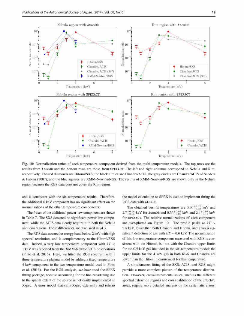
Publications of the Astronomical Society of Japan, (2014), Vol. 00, No. 0 19
0 2 4 6 8Temperature (keV)
10−3
10−2
10−1
100Normalizationratio
Nebula region with AtomDB
Hitomi/SXS
Chandra/ACIS
Chandra/ACIS (S07)
XMM-Newton/RGS
0 2 4 6 8Temperature (keV)
10−3
10−2
10−1
100
Normalizationratio
Rim region with AtomDB
Hitomi/SXS
Chandra/ACIS
Chandra/ACIS (S07)
0 2 4 6 8Temperature (keV)
10−3
10−2
10−1
100
Normalizationratio
Nebula region with SPEXACT
Hitomi/SXS
Chandra/ACIS
XMM-Newton/RGS
0 2 4 6 8Temperature (keV)
10−3
10−2
10−1
100
Normalizationratio
Rim region with SPEXACT
Hitomi/SXS
Chandra/ACIS
Fig. 10: Normalization ratios of each temperature component derived from the multi-temperature models. The top rows are the
results from AtomdB and the bottom rows are those from SPEXACT. The left and right columns correspond to Nebula and Rim,
respectively. The red diamonds are Hitomi/SXS, the black circles are Chandra/ACIS, the gray circles are Chandra/ACIS of Sanders
& Fabian (2007), and the blue squares are XMM-Newton/RGS. The results of XMM-Newton/RGS are shown only in the Nebula
region because the RGS data does not cover the Rim region.
and is consistent with the six-temperature results. Therefore,
the additional 6 keV component has no significant effect on the
normalizations of the other temperature components.
The fluxes of the additional power-law component are shown
in Table 7. The SXS detected no significant power-law compo-
nent, while the ACIS data clearly require it in both the Nebula
and Rim regions. These differences are discussed in §4.3.
The RGS data covers the energy band below 2 keV with high
spectral resolution, and is complementary to the Hitomi/SXS
data. Indeed, a very low temperature component with kT <
1 keV was reported from the XMM-Newton/RGS observations
(Pinto et al. 2016). Here, we fitted the RGS spectrum with a
three-temperature plasma model by adding a fixed-temperature
4 keV component to the two-temperature model used in Pinto
et al. (2016). For the RGS analysis, we have used the SPEX
fitting package, because accounting for the line broadening due
to the spatial extent of the source is not easily implemented in
Xspec. A user model that calls Xspec externally and returns
the model calculation to SPEX is used to implement fitting the
RGS data with AtomDB.
The obtained best-fit temperatures are 0.60+0.02−0.02 keV and
2.7+0.08−0.05 keV for AtomDB and 0.55+0.03
−0.06 keV and 2.4+0.08−0.10 keV
for SPEXACT. The relative normalizations of each component
are over-plotted on Figure 10. The profile peaks at kT ∼
2.5 keV, lower than both Chandra and Hitomi, and gives a sig-
nificant detection of gas with kT ∼ 0.6 keV. The normalization
of this low temperature component measured with RGS is con-
sistent with the Hitomi, but not with the Chandra upper limits
for the 0.5 keV gas included in the six-temperature model; the
upper limits for the 4 keV gas in both RGS and Chandra are
lower than the Hitomi measurement for this temperature.
A simultaneous fitting of the SXS, ACIS, and RGS might
provide a more complete picture of the temperature distribu-
tion. However, cross-instruments issues, such as the different
spectral extraction regions and cross calibration of the effective
areas, require more detailed analysis on the systematic errors.
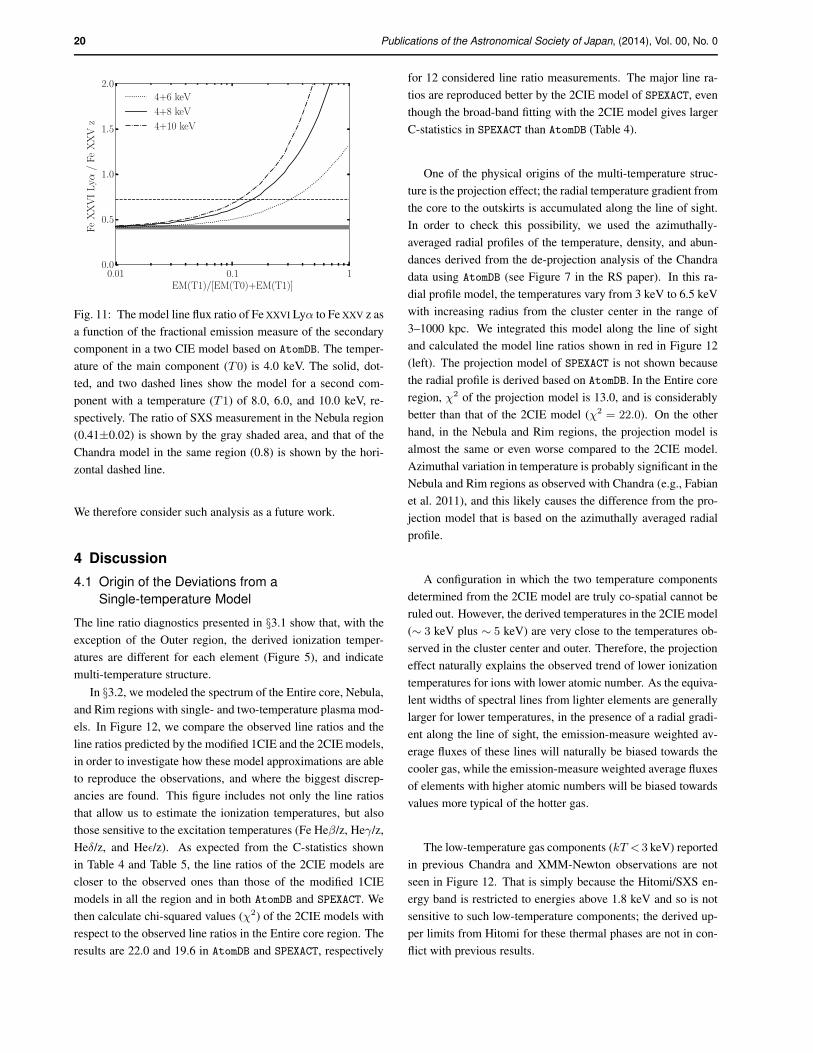
20 Publications of the Astronomical Society of Japan, (2014), Vol. 00, No. 0
0.01 0.1 1EM(T1)/[EM(T0)+EM(T1)]
0.0
0.5
1.0
1.5
2.0FeXXVILyα
/FeXXVz
4+6 keV
4+8 keV
4+10 keV
Fig. 11: The model line flux ratio of Fe XXVI Lyα to Fe XXV z as
a function of the fractional emission measure of the secondary
component in a two CIE model based on AtomDB. The temper-
ature of the main component (T0) is 4.0 keV. The solid, dot-
ted, and two dashed lines show the model for a second com-
ponent with a temperature (T1) of 8.0, 6.0, and 10.0 keV, re-
spectively. The ratio of SXS measurement in the Nebula region
(0.41±0.02) is shown by the gray shaded area, and that of the
Chandra model in the same region (0.8) is shown by the hori-
zontal dashed line.
We therefore consider such analysis as a future work.
4 Discussion
4.1 Origin of the Deviations from a
Single-temperature Model
The line ratio diagnostics presented in §3.1 show that, with the
exception of the Outer region, the derived ionization temper-
atures are different for each element (Figure 5), and indicate
multi-temperature structure.
In §3.2, we modeled the spectrum of the Entire core, Nebula,
and Rim regions with single- and two-temperature plasma mod-
els. In Figure 12, we compare the observed line ratios and the
line ratios predicted by the modified 1CIE and the 2CIE models,
in order to investigate how these model approximations are able
to reproduce the observations, and where the biggest discrep-
ancies are found. This figure includes not only the line ratios
that allow us to estimate the ionization temperatures, but also
those sensitive to the excitation temperatures (Fe Heβ/z, Heγ/z,
Heδ/z, and Heǫ/z). As expected from the C-statistics shown
in Table 4 and Table 5, the line ratios of the 2CIE models are
closer to the observed ones than those of the modified 1CIE
models in all the region and in both AtomDB and SPEXACT. We
then calculate chi-squared values (χ2) of the 2CIE models with
respect to the observed line ratios in the Entire core region. The
results are 22.0 and 19.6 in AtomDB and SPEXACT, respectively
for 12 considered line ratio measurements. The major line ra-
tios are reproduced better by the 2CIE model of SPEXACT, even
though the broad-band fitting with the 2CIE model gives larger
C-statistics in SPEXACT than AtomDB (Table 4).
One of the physical origins of the multi-temperature struc-
ture is the projection effect; the radial temperature gradient from
the core to the outskirts is accumulated along the line of sight.
In order to check this possibility, we used the azimuthally-
averaged radial profiles of the temperature, density, and abun-
dances derived from the de-projection analysis of the Chandra
data using AtomDB (see Figure 7 in the RS paper). In this ra-
dial profile model, the temperatures vary from 3 keV to 6.5 keV
with increasing radius from the cluster center in the range of
3–1000 kpc. We integrated this model along the line of sight
and calculated the model line ratios shown in red in Figure 12
(left). The projection model of SPEXACT is not shown because
the radial profile is derived based on AtomDB. In the Entire core
region, χ2 of the projection model is 13.0, and is considerably
better than that of the 2CIE model (χ2 = 22.0). On the other
hand, in the Nebula and Rim regions, the projection model is
almost the same or even worse compared to the 2CIE model.
Azimuthal variation in temperature is probably significant in the
Nebula and Rim regions as observed with Chandra (e.g., Fabian
et al. 2011), and this likely causes the difference from the pro-
jection model that is based on the azimuthally averaged radial
profile.
A configuration in which the two temperature components
determined from the 2CIE model are truly co-spatial cannot be
ruled out. However, the derived temperatures in the 2CIE model
(∼ 3 keV plus ∼ 5 keV) are very close to the temperatures ob-
served in the cluster center and outer. Therefore, the projection
effect naturally explains the observed trend of lower ionization
temperatures for ions with lower atomic number. As the equiva-
lent widths of spectral lines from lighter elements are generally
larger for lower temperatures, in the presence of a radial gradi-
ent along the line of sight, the emission-measure weighted av-
erage fluxes of these lines will naturally be biased towards the
cooler gas, while the emission-measure weighted average fluxes
of elements with higher atomic numbers will be biased towards
values more typical of the hotter gas.
The low-temperature gas components (kT <3 keV) reported
in previous Chandra and XMM-Newton observations are not
seen in Figure 12. That is simply because the Hitomi/SXS en-
ergy band is restricted to energies above 1.8 keV and so is not
sensitive to such low-temperature components; the derived up-
per limits from Hitomi for these thermal phases are not in con-
flict with previous results.
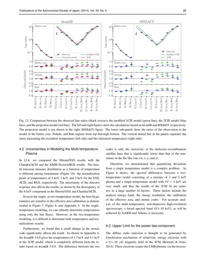
Publications of the Astronomical Society of Japan, (2014), Vol. 00, No. 0 21
10−1
100
101Lineratios
Entire core
AtomDB
Observed
Projection model
modified 1CIE
2CIE
0.5
1.0
1.5 Entire core
0.5
1.0
1.5
Observed/M
odel
Nebula
FeHeβ
/z
FeHeγ/z
FeHeδ/z
FeHeǫ/z
SiLyα
/w
SLyα
/w
ArLyα
/w
CaLyα
/w
FeLyα
/z
FeLyα
/Heβ
FeLyα
/Heγ
FeLyα
/Heδ
FeLyα
/Heǫ
0.5
1.0
1.5 Rim
10−1
100
101
Lineratios
Entire core
SPEXACT
Observed
modified 1CIE
2CIE
0.5
1.0
1.5 Entire core
0.5
1.0
1.5
Observed/M
odel
Nebula
FeHeβ
/z
FeHeγ/z
FeHeδ/z
FeHeǫ/z
SiLyα
/w
SLyα
/w
ArLyα
/w
CaLyα
/w
FeLyα
/z
FeLyα
/Heβ
FeLyα
/Heγ
FeLyα
/Heδ
FeLyα
/Heǫ
0.5
1.0
1.5 Rim
Fig. 12: Comparison between the observed line ratios (black crosses), the modified 1CIE model (green line), the 2CIE model (blue
line), and the projection model (red line). The left and right figures show the calculations based on AtomDB and SPEXACT, respectively.
The projection model is not shown in the right (SPEXACT) figure. The lower sub-panels show the ratios of the observation to the
model in the Entire core, Nebula, and Rim regions from top thorough bottom. The vertical dotted line in the panels separates the
ratios measuring the excitation temperature (left side) and the ionization temperature (right side).
4.2 Uncertainties in Modeling the Multi-temperature
Plasma
In §3.4, we compared the Hitomi/SXS results with the
Chandra/ACIS and the XMM-Newton/RGS results. The best-
fit emission measure distribution as a function of temperature
is different among instruments (Figure 10): the normalization
peaks at temperatures of 4 keV, 3 keV, and 2 keV for the SXS,
ACIS, and RGS, respectively. The uncertainty of the detector
response also affects the results, as shown by the discrepancy of
the 8 keV component in the Hitomi/SXS and Chandra/ACIS.
Even in the single- or two-temperature model, the best-fit pa-
rameters are sensitive to the effective area calibration as demon-
strated in Figure 7, Figure 8, and Appendix 4. In the single-
temperature modeling, we can robustly determine temperatures
using only the line fluxes. However, in the two-temperature
modeling, it is difficult to determine both temperatures and nor-
malizations exactly.
Furthermore, we found that a small change in the atomic
code significantly affects the result. As shown in Appendix 6,
the AtomDB 3.0.8 gives the temperatures of 1.7 keV and 4.1 keV
in the 2CIE model, which is completely different from the re-
sults based on AtomDB 3.0.9. The difference between the two
codes is only the emissivity of the dielectric-recombination
satellite lines that is significantly lower than that of the tran-
sitions in the He-like ions (w, x, y, and z).
Therefore, we demonstrated that quantifying deviations
from a single temperature model is a complex problem. As
Figure 6 shows, the spectral differences between a two-
temperature model consisting of a mixture of 3 and 5 keV
plasma and a single-temperature model with kT = 4 keV are
very small, and thus the results of the 2CIE fit are sensi-
tive to a large number of factors. These factors include the
analysis energy band, the energy resolution, the calibration
of the effective area, and atomic codes. For accurate anal-
ysis of the multi-temperature, non-dispersive high-resolution
spectroscopy, a broad spectral band (0.5–10 keV), as will be
achieved by XARM and Athena, is necessary.
4.3 Upper Limit for the power-law component
The diffuse radio emission is thought to be generated by
Synchrotron mechanism of relativistic energy electrons with
a 0.1–10 µG magnetic field in the ICM (Brunetti & Jones
2014). These electrons scatter the CMB photons via the inverse-
22 Publications of the Astronomical Society of Japan, (2014), Vol. 00, No. 0
Compton scattering, which allows us to investigate the mag-
netic field in the ICM (Ota 2012). Based on an assumption
that inverse-Compton emission is generated by the same pop-
ulation of relativistic electrons, the volume-integrated magnetic
field strength can be derived from intensities/upper-limits of IC
emission (Rybicki & Lightman 1979).
Sanders & Fabian (2007) reported the detection of a diffuse
power-law component in the core of the Perseus cluster, which
was not confirmed by the XMM-Newton analysis (Molendi &
Gastaldello 2009). The corresponding surface brightness in
the 2–10 keV band measured by Sanders & Fabian (2007) is
∼15×10−16 and ∼8×10⁻¹⁶ erg cm−2 s−1 arcsec−2 in Nebula
and Rim, respectively. Our reanalysis of the Chandra/ACIS data
also suggests the presence of such a power-law component, but
with observed fluxes lower by a factor of 2–4 in better agree-
ment with the upper limit of 5× 10⁻¹⁶ erg cm−2 s−1 arcsec−2
reported by Molendi & Gastaldello 2009. That is likely
caused by the update of the calibration database described in
Nevalainen et al. (2010); the response for the higher energy
band is improved and significantly reduces the flux in that en-
ergy band.
In contrast, the Hitomi/SXS results show upper limits for
this power-law component that are significantly lower than the
fluxes measured with Chandra/ACIS.. As shown in Figure
9, large systematic residuals are present above 5 keV in the
Chandra spectra even after the update of the effective area cali-
bration, and they likely bias the power-law fluxes. A similar dis-
crepancy was also reported in the comparison with the XMM-
Newton/EPIC results (Molendi & Gastaldello 2009). Since the
Hitomi/SXS covers a wider energy range up to 20 keV, the ob-
tained upper limits would be robust at least in the Rim region,
in which the level of the AGN contamination is low.
Assuming the power-law component is due to inverse-
Compton scattering, we can estimate the strength of the mag-
netic field (B) as discussed in Sanders et al. (2005). Using
the SXS upper limit of < 1.2× 10⁻¹⁶ erg cm−2 s−1 arcsec2
in the Rim region, we obtained the lower limit of B > 0.4 µG.
This value is consistent with the results of other observations
performed at other wavelengths (∼7–25 µG) as discussed in
Molendi & Gastaldello (2009).
5 Conclusion
Compared to the intricate structures revealed by the deep
Chandra image of the core of the Perseus Cluster (e.g, Fabian
et al. 2011), at first glance the high-quality Hitomi SXS spec-
tra of this source, which are sensitive to the temperature range
of >∼ 3 keV, present a surprisingly quiescent view: the velocity
dispersions are rather small (the First paper, the V paper), the
chemical composition is remarkably similar to the solar neigh-
borhood (the Z paper), and the spectra between 1.8–20 keV are
largely well approximated by a single temperature model. The
diffuse power-law component reported from previous Chandra
measurements is also not required by the Hitomi data.
We have resolved line emission from various ions. This pro-
vides the first direct measurements of the electron temperature
and ionization degree separately from different transitions of
He-like and H-like ions of Si, S, Ar, Ca, and Fe. Compared
with previous temperature measurements mostly based on the
continuum shape, the new diagnostics are more sensitive to ex-
citation processes and plasma conditions. We found that all ob-
served ratios are broadly consistent with the CIE approxima-
tion. However, there are two signs of small deviation from a
single temperature model. Firstly there is a trend of increas-
ing ionization temperature with increasing atomic mass, partic-
ularly in the Nebula (central) region and possibly also in the
surrounding Rim region. Secondly, the excitation temperature
from Fe (∼ 3 keV) is lower than the corresponding ionization
temperature and than the electron temperature determined from
the spectral continuum (∼ 4 keV) for the Nebula. In the Nebula
and Rim regions, the best-fit two temperature models suggest a
mix of roughly 3 and 5 keV plasma, both of which are expected
to be present based on deprojected temperature profiles previ-
ously measured with Chandra. On the other hand, the Outer
region, corresponding to the farthest observation from the clus-
ter core performed by Hitomi, shows no significant deviation
from single temperature. No additional third temperature com-
ponent, Gaussian nor power-law DEM model, nor significant
emission from non-equilibrium ionization plasma are required
to describe the spectra.
Even though we can not rule out a true multi-phase struc-
ture in which different temperature components are co-spatial,
the projection effect is a natural explanation for the observed
deviations from single temperature.
Best-fit models of lower-resolution spectra that include the
energy band below 2 keV and the RGS spectra seem to present
a contrasting picture, requiring a multi-phase thermal structure
that the Hitomi observations are currently not sensitive to. It
is clear that the dominant thermal component in the spectral fit
depends on the energy band observed, and that detectors able to
cover simultaneously the emission lines from all phases of the
ICM are needed in order for a reliable temperature structure to
be pinned down. High-resolution, non-dispersive spectroscopy
with XARM or Athena will thus be crucial in order to assess
the origins and robustness of the multi-temperature structure re-
ported by CCD studies, and verify to what extent the complexity
of cluster cores revealed by high-spatial resolution images cor-
responds to an equally complex picture along the energy axis.
Author contributions
S. Nakashima led this study in data analysis and wrote the manuscript. K.
Matsushita, A. Simionescu, and T. Tamura reviewed the manuscript fully.
Publications of the Astronomical Society of Japan, (2014), Vol. 00, No. 0 23
K. Sato and T. Tamura performed a cross-check of the Hitomi/SXS analy-
sis. Y. Kato analyzed the Chandra/ACIS archival data. A. Simionescu and
N. Werner performed the XMM-Newton/RGS analysis. M. Furukawa and
K. Sato constructed the projection model and checked the effect of the res-
onance scattering. M. Bautz, H. Akamatsu, M. Tsujimoto, H. Yamaguchi,
K. Makishima, C. Pinto, Y. Fukazawa, R. Mushotzky, and J. de Plaa pro-
vided valuable comments that improved the draft. S. Nakashima, K, Sato,
K. Nakazawa, T. Okajima, and N. Yamasaki contributed to fabrication of
the instruments and performed the in-orbit operation and calibration.
Acknowledgments
We are thankful for the support from the JSPS Core-to-Core Program.
We acknowledge all the JAXA members who have contributed to the
ASTRO-H (Hitomi) project. All U.S. members gratefully acknowl-
edge support through the NASA Science Mission Directorate. Stanford
and SLAC members acknowledge support via DoE contract to SLAC
National Accelerator Laboratory DE-AC3-76SF00515. Part of this work
was performed under the auspices of the U.S. DoE by LLNL under
Contract DE-AC52-07NA27344. Support from the European Space
Agency is gratefully acknowledged. French members acknowledge sup-
port from CNES, the Centre National d’Etudes Spatiales. SRON is sup-
ported by NWO, the Netherlands Organization for Scientific Research.
Swiss team acknowledges support of the Swiss Secretariat for Education,
Research and Innovation (SERI). The Canadian Space Agency is ac-
knowledged for the support of Canadian members. We acknowl-
edge support from JSPS/MEXT KAKENHI grant numbers 15J02737,
15H00773, 15H00785, 15H02090, 15H03639, 15H05438, 15K05107,
15K17610, 15K17657, 16J00548, 16J02333, 16H00949, 16H06342,
16K05295, 16K05296, 16K05300, 16K13787, 16K17672, 16K17673,
21659292, 23340055, 23340071, 23540280, 24105007, 24244014,
24540232, 25105516, 25109004, 25247028, 25287042, 25400236,
25800119, 26109506, 26220703, 26400228, 26610047, 26800102,
JP15H02070, JP15H03641, JP15H03642, JP15H06896, JP16H03983,
JP16K05296, JP16K05309, JP16K17667, and JP16K05296. The follow-
ing NASA grants are acknowledged: NNX15AC76G, NNX15AE16G,
NNX15AK71G, NNX15AU54G, NNX15AW94G, and NNG15PP48P
to Eureka Scientific. H. Akamatsu acknowledges support of NWO
via Veni grant. C. Done acknowledges STFC funding under grant
ST/L00075X/1. A. Fabian and C. Pinto acknowledge ERC Advanced
Grant 340442. P. Gandhi acknowledges JAXA International Top Young
Fellowship and UK Science and Technology Funding Council (STFC)
grant ST/J003697/2. Y. Ichinohe, K. Nobukawa, and H. Seta are sup-
ported by the Research Fellow of JSPS for Young Scientists. N. Kawai
is supported by the Grant-in-Aid for Scientific Research on Innovative
Areas “New Developments in Astrophysics Through Multi-Messenger
Observations of Gravitational Wave Sources”. S. Kitamoto is partially
supported by the MEXT Supported Program for the Strategic Research
Foundation at Private Universities, 2014-2018. B. McNamara and S.
Safi-Harb acknowledge support from NSERC. T. Dotani, T. Takahashi,
T. Tamagawa, M. Tsujimoto and Y. Uchiyama acknowledge support from
the Grant-in-Aid for Scientific Research on Innovative Areas “Nuclear
Matter in Neutron Stars Investigated by Experiments and Astronomical
Observations”. N. Werner is supported by the Lendulet LP2016-11 grant
from the Hungarian Academy of Sciences. D. Wilkins is supported by
NASA through Einstein Fellowship grant number PF6-170160, awarded
by the Chandra X-ray Center, operated by the Smithsonian Astrophysical
Observatory for NASA under contract NAS8-03060.
We are grateful for contributions by many companies, including
in particular, NEC, Mitsubishi Heavy Industries, Sumitomo Heavy
Industries, and Japan Aviation Electronics Industry. Finally, we ac-
knowledge strong support from the following engineers. JAXA/ISAS:
Chris Baluta, Nobutaka Bando, Atsushi Harayama, Kazuyuki Hirose,
Kosei Ishimura, Naoko Iwata, Taro Kawano, Shigeo Kawasaki, Kenji
Minesugi, Chikara Natsukari, Hiroyuki Ogawa, Mina Ogawa, Masayuki
Ohta, Tsuyoshi Okazaki, Shin-ichiro Sakai, Yasuko Shibano, Maki Shida,
Takanobu Shimada, Atsushi Wada, Takahiro Yamada; JAXA/TKSC:
Atsushi Okamoto, Yoichi Sato, Keisuke Shinozaki, Hiroyuki Sugita;
Chubu U: Yoshiharu Namba; Ehime U: Keiji Ogi; Kochi U of
Technology: Tatsuro Kosaka; Miyazaki U: Yusuke Nishioka; Nagoya
U: Housei Nagano; NASA/GSFC: Thomas Bialas, Kevin Boyce, Edgar
Canavan, Michael DiPirro, Mark Kimball, Candace Masters, Daniel
Mcguinness, Joseph Miko, Theodore Muench, James Pontius, Peter
Shirron, Cynthia Simmons, Gary Sneiderman, Tomomi Watanabe;
ADNET Systems: Michael Witthoeft, Kristin Rutkowski, Robert S. Hill,
Joseph Eggen; Wyle Information Systems: Andrew Sargent, Michael
Dutka; Noqsi Aerospace Ltd: John Doty; Stanford U/KIPAC: Makoto
Asai, Kirk Gilmore; ESA (Netherlands): Chris Jewell; SRON: Daniel
Haas, Martin Frericks, Philippe Laubert, Paul Lowes; U of Geneva:
Philipp Azzarello; CSA: Alex Koujelev, Franco Moroso.
References
Akamatsu, H., & Kawahara, H. 2013, PASJ, 65, 16
Arnaud, K. A. 1996, in Astronomical Society of the Pacific Conference
Series, Vol. 101, Astronomical Data Analysis Software and Systems
V, ed. G. H. Jacoby & J. Barnes, 17
Arnaud, M., Pratt, G. W., Piffaretti, R., et al. 2010, A&A, 517, A92
Brunetti, G., & Jones, T. W. 2014, International Journal of Modern
Physics D, 23, 1430007
Bulbul, E., Markevitch, M., Foster, A., et al. 2014, ApJ, 789, 13
Cash, W. 1979, ApJ, 228, 939
Churazov, E., Forman, W., Jones, C., & Bohringer, H. 2003, ApJ, 590,
225
Conselice, C. J., Gallagher, III, J. S., & Wyse, R. F. G. 2001, AJ, 122,
2281
de Plaa, J., Werner, N., Bleeker, J. A. M., et al. 2007, A&A, 465, 345
de Plaa, J., Kaastra, J. S., Werner, N., et al. 2017, ArXiv e-prints,
arXiv:1707.05076
Eckart, M. E., Adams, J. S., Boyce, K. R., et al. 2017, Journal of
Astronomical Telescopes, Instruments, and Systems
Fabian, A. C., Sanders, J. S., Allen, S. W., et al. 2011, MNRAS, 418,
2154
Foster, A. R., Ji, L., Smith, R. K., & Brickhouse, N. S. 2012, ApJ, 756,
128
Fujita, Y., Kimura, S., & Ohira, Y. 2013, MNRAS, 432, 1434
Fujita, Y., Hayashida, K., Nagai, M., et al. 2008, PASJ, 60, 1133
Fukazawa, Y., Ohashi, T., Fabian, A. C., et al. 1994, PASJ, 46, L55
Gu, L., Xu, H., Gu, J., et al. 2012, ApJ, 749, 186
Gu, L., Gandhi, P., Inada, N., et al. 2013, ApJ, 767, 157
Hitomi Collaboration. 2016, Nature, 535, 117
—. 2017, ApJL, 837, L15
Inoue, S., Hayashida, K., Ueda, S., et al. 2016, PASJ, 68, S23
Kaastra, J. S. 2017, ArXiv e-prints, arXiv:1707.09202
Kaastra, J. S., Mewe, R., & Nieuwenhuijzen, H. 1996, in UV and
X-ray Spectroscopy of Astrophysical and Laboratory Plasmas, ed.
K. Yamashita & T. Watanabe, 411–414
Kaastra, J. S., Tamura, T., Peterson, J. R., et al. 2004, A&A, 413, 415
24 Publications of the Astronomical Society of Japan, (2014), Vol. 00, No. 0
Kalberla, P. M. W., Burton, W. B., Hartmann, D., et al. 2005, A&A, 440,
775
Kilbourne, C. A., Sawada, M., Tsujimoto, M., et al. 2017, PASJ
Leccardi, A., & Molendi, S. 2008, A&A, 486, 359
Madsen, K. K., Reynolds, S., Harrison, F., et al. 2015, ApJ, 801, 66
Makishima, K., Ezawa, H., Fukuzawa, Y., et al. 2001, PASJ, 53, 401
Markevitch, M., & Vikhlinin, A. 2007, Phys. Rep., 443, 1
Markevitch, M., Ponman, T. J., Nulsen, P. E. J., et al. 2000, ApJ, 541, 542
Matsushita, K., Belsole, E., Finoguenov, A., & Bohringer, H. 2002, A&A,
386, 77
McNamara, B. R., & Nulsen, P. E. J. 2007, ARA&A, 45, 117
Molendi, S., & Gastaldello, F. 2009, A&A, 493, 13
Nevalainen, J., David, L., & Guainazzi, M. 2010, A&A, 523, A22
Okajima, T., Soong, Y., Serlemitsos, P., et al. 2016, in Proc. SPIE, Vol.
9905, Society of Photo-Optical Instrumentation Engineers (SPIE)
Conference Series, 99050Z
Ota, N. 2012, Research in Astronomy and Astrophysics, 12, 973
Peterson, J. R., Kahn, S. M., Paerels, F. B. S., et al. 2003, ApJ, 590, 207
Pinto, C., Fabian, A. C., Ogorzalek, A., et al. 2016, MNRAS, 461, 2077
Planck Collaboration, Ade, P. A. R., Aghanim, N., et al. 2013, A&A, 550,
A131
Rybicki, G. B., & Lightman, A. P. 1979, Radiative processes in
astrophysics
Sanders, J. S., & Fabian, A. C. 2007, MNRAS, 381, 1381
Sanders, J. S., Fabian, A. C., & Dunn, R. J. H. 2005, MNRAS, 360, 133
Sanders, J. S., Fabian, A. C., Taylor, G. B., et al. 2016, MNRAS, 457, 82
Sato, T., Matsushita, K., Ota, N., et al. 2011, PASJ, 63, S991
Schellenberger, G., Reiprich, T. H., Lovisari, L., Nevalainen, J., & David,
L. 2015, A&A, 575, A30
Simionescu, A., Werner, N., Bohringer, H., et al. 2009, A&A, 493, 409
Simionescu, A., Werner, N., Mantz, A., Allen, S. W., & Urban, O. 2017,
MNRAS, 469, 1476
Simionescu, A., Allen, S. W., Mantz, A., et al. 2011, Science, 331, 1576
Takahashi, I., Kawaharada, M., Makishima, K., et al. 2009, ApJ, 701, 377
Tsujimoto, M., Okajima, T., Kilbourne, C. A., et al. 2017, PASJ
Vikhlinin, A., Markevitch, M., & Murray, S. S. 2001, ApJ, 551, 160
Wilms, J., Allen, A., & McCray, R. 2000, ApJ, 542, 914
Appendix 1 Gain Correction
We checked uncertainties of the gain scale of the SXS and cor-
rected them using the Perseus data themselves, because the gain
scale calibration is limited due to the short life of Hitomi. The
procedure described in this section is essentially the same as
that used in the Z paper and Atomic paper, except that the refer-
ence redshift was changed from 0.01756 to 0.017284 according
to the V paper.
We first applied a linear gain shift for each pixel in each ob-
servation so that the apparent energies of the Fe XXV lines agree
with a redshift of 0.017284. The resulting amount of the energy
shift at 6.5 keV is 1.0±1.9 eV (mean and standard deviation).
This pixel-by-pixel redshift correction removes not only the re-
maining gain errors among pixels but also the spatial variation
of the Doppler shift for the ICM. Our results are not affected by
this possible “over-correction”.
We then co-added spectra of all the pixels for each observa-
tion and investigated the energy shifts of each line in the 1.8–9.0
keV band. Figure 13 summarizes the differences of line ener-
gies from the fiducial values assuming a redshift of 0.017284.
We modeled these data by the parabolic function shown below,
in which ∆E at E = 6586.5 eV was constrained to zero:
Ecor = E+ a× (E− 6586.5) + b× (E− 6586.5)2 eV. (A1)
The obtained parameters are
a=−4.888× 10⁻⁴ and b= 2.035× 10⁻⁶, (A2)
a = 4.303× 10⁻⁴ and b= 2.390× 10⁻⁴, (A3)
a = 6.250× 10⁻⁴ and b= 2.702× 10⁻⁴, (A4)
a = 8.640× 10⁻⁴ and b= 3.439× 10⁻⁴, (A5)
for obs1, obs2, obs3, and obs4, respectively. We applied these
corrections to all the pixels. As confirmed in Figure 6 of the
RS paper, these gain corrections have no impact on the line
flux measurement, which is crucial for the temperature mea-
surements.
Appendix 2 Detailed best-fit parameters ofthe Gaussian fits
The centers and widths derived from the Gaussian fits in §3.1
are shown in Table 8. The obtained line widths are consistent
with the results described in V paper.
Appendix 3 Single-line based emissionmeasure limits
In Figure 14, we show theoretical emissivities for some of ob-
served line transitions as a function of electron temperature
based on AtomDB. The peak temperature, where the emissivity
becomes maximum, from these ions cover a temperature range
from 1.5 keV (H-like Si) to 13 keV (H-like Fe). Therefore mea-
surements of line fluxes and ratios are sensitive to emission from
plasma at around this temperature range.
Combined with these emissivity values, the observed flux for
each transition (Table 3) provides constrains on emission mea-
sure for a given temperature and a metal abundance, as shown
in Figure 14. If the line emission originate from a single com-
ponent CIE plasma any two curves from a single element cross
at a single point of the model temperature and emission mea-
sure. Furthermore, if the assumed metal abundances are cor-
rect, curves from different elements also cross at a single point.
Our measured profiles from the entire core intersect together
at around 3–4 keV, indicating that the observed line fluxes and
hence their ratios can be approximated by a single component
CIE plasma with the solar abundance ratios. From these curves
we notice that the Fe XXVI Lyα is the most sensitive to hotter
(> 4 keV) emission and He-like S and Ar lines are the most
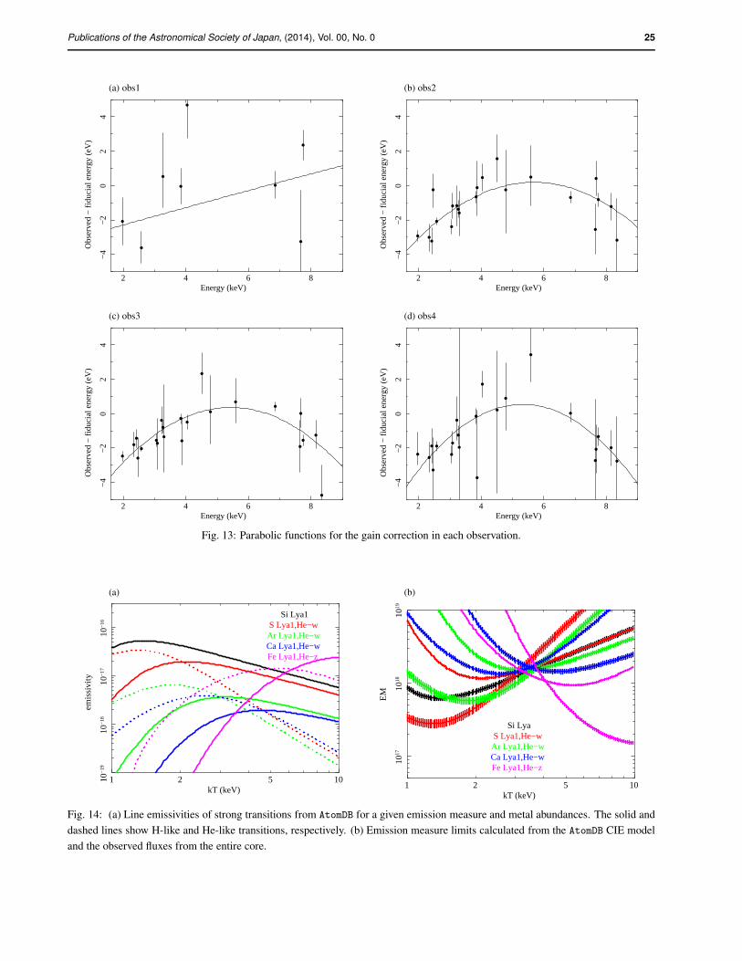
Publications of the Astronomical Society of Japan, (2014), Vol. 00, No. 0 25
(a) obs1
2 4 6 8
−4
−2
02
4
Obs
erve
d −
fidu
cial
ene
rgy
(eV
)
Energy (keV)
(b) obs2
2 4 6 8
−4
−2
02
4
Obs
erve
d −
fidu
cial
ene
rgy
(eV
)
Energy (keV)
(c) obs3
2 4 6 8
−4
−2
02
4
Obs
erve
d −
fidu
cial
ene
rgy
(eV
)
Energy (keV)
(d) obs4
2 4 6 8
−4
−2
02
4
Obs
erve
d −
fidu
cial
ene
rgy
(eV
)
Energy (keV)
Fig. 13: Parabolic functions for the gain correction in each observation.
(a)
1 102 510−
1910
−18
10−
1710
−16
emis
sivi
ty
kT (keV)
Si Lya1S Lya1,He−wAr Lya1,He−wCa Lya1,He−wFe Lya1,He−z
(b)
1 102 5
1017
1018
1019
EM
kT (keV)
Si LyaS Lya1,He−wAr Lya1,He−wCa Lya1,He−wFe Lya1,He−z
Fig. 14: (a) Line emissivities of strong transitions from AtomDB for a given emission measure and metal abundances. The solid and
dashed lines show H-like and He-like transitions, respectively. (b) Emission measure limits calculated from the AtomDB CIE model
and the observed fluxes from the entire core.
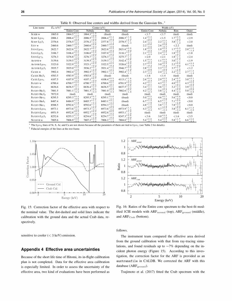
26 Publications of the Astronomical Society of Japan, (2014), Vol. 00, No. 0
Table 8: Observed line centers and widths derived from the Gaussian fits..∗
Line name E0 (eV)† Center (eV) Width (eV)
Entire Core Nebula Rim Outer Entire Core Nebula Rim Outer
Si XIII w 1865.0 1864.5+1.1
−1.01864.3
+1.9
−0.9(fixed) (fixed) <1.7 <1.7 (tied) (tied)
Si XIV Lyα1 2006.1 2006.4+0.3
−0.22006.5
+0.3
−0.22006.4
+0.4
−0.32006.5
+1.2
−1.31.4
+0.3
−0.3<1.5 1.7
+0.5
−0.5<2.9
Si XIV Lyβ1 2376.6 2376.5+0.5
−0.52376.2
+0.5
−0.52377.8
+1.3
−1.42378.5
+1.1
−1.32.4
+0.5
−0.52.2
+0.5
−0.53.8
+1.3
−1.2<2.0
S XV w 2460.6 2460.7+0.5
−0.32460.6
+0.6
−0.42460.7
+0.8
−0.6(fixed) 2.2
+0.6
−0.62.6
+0.8
−0.7<2.2 (tied)
S XVI Lyα1 2622.7 2622.6+0.1
−0.12622.7
+0.1
−0.22622.6
+0.2
−0.22621.6
+0.9
−0.91.8
+0.2
−0.21.9
+0.2
−0.21.7
+0.3
−0.32.0
+1.0
−1.2
S XVI Lyβ1 3106.7 3106.4+0.3
−0.33106.0
+0.4
−0.43107.0
+0.3
−0.53116.1
+0.7
−1.32.1
+0.4
−0.32.4
+0.5
−0.41.8
+0.5
−0.7<1.8
S XVI Lyγ1 3276.3 3276.8+0.3
−0.83276.7
+0.5
−0.83276.3
+1.0
−0.83275.7
+1.4
−1.4<2.0 <2.1 1.8
+1.2
−1.4<2.4
Ar XVII w 3139.6 3139.5+0.3
−0.33139.5
+0.3
−0.43139.3
+1.2
−1.13142.4
+0.8
−1.01.5
+0.4
−0.41.1
+0.5
−0.63.0
+1.4
−1.1<1.9
Ar XVIII Lyα1 3323.0 3322.9+0.2
−0.33323.1
+0.3
−0.43322.5
+0.5
−0.43326.6
+2.2
−2.22.7
+0.4
−0.43.0
+0.4
−0.42.2
+0.6
−0.64.1
+2.3
−1.6
Ar XVIII Lyβ1 3935.7 3935.0+0.9
−1.03936.2
+0.7
−1.33931.4
+1.5
−1.73946.7
+0.6
−1.22.8
+1.0
−0.82.3
+1.0
−0.93.7
+1.7
−1.6<1.2
Ca XIX w 3902.4 3902.4+0.2
−0.23902.5
+0.2
−0.33902.1
+0.3
−0.43902.4
+1.5
−1.12.3
+0.2
−0.22.4
+0.3
−0.32.2
+0.4
−0.42.7
+1.5
−1.2
Ca XIX Heβ1 4583.5 4583.9+0.4
−0.94583.8
+0.2
−0.9(fixed) (fixed) <1.6 <1.4 (tied) (tied)
Ca XX Lyα1 4107.5 4107.9+0.3
−0.54107.1
+0.7
−0.44108.4
+0.5
−0.64113.1
+1.8
−1.52.6
+0.4
−0.42.9
+0.5
−0.52.4
+0.7
−0.63.0
+2.1
−1.2
Fe XXV w 6700.4 6700.7+0.0
−0.16700.7
+0.1
−0.16700.6
+0.1
−0.16701.9
+0.4
−0.24.2
+0.1
−0.14.3
+0.1
−0.14.0
+0.1
−0.14.3
+0.2
−0.2
Fe XXV z 6636.6 6636.5+0.1
−0.16636.4
+0.2
−0.16636.5
+0.1
−0.26637.5
+0.5
−0.53.4
+0.1
−0.13.6
+0.1
−0.13.2
+0.2
−0.23.9
+0.5
−0.5
Fe XXV Heβ1 7881.5 7881.1+0.2
−0.27881.3+0.3
−0.37881.0+0.3
−0.37882.6+0.5
−1.84.2+0.2
−0.33.8+0.3
−0.44.4+0.3
−0.35.0+0.9
−0.8
Fe XXV Heβ2 7872.0 (tied) (tied) (tied) (tied) (tied) (tied) (tied) (tied)
Fe XXV Heγ1 8295.5 8295.3+0.4
−0.68295.5
+0.7
−0.78295.1
+0.6
−1.1(fixed) 5.0
+0.5
−0.54.6
+0.7
−0.65.6
+0.8
−0.7<0.0
Fe XXV Heδ1 8487.4 8484.9+1.4
−1.28485.7
+1.7
−1.78483.1
+2.1
−1.7(fixed) 6.7
+1.3
−1.06.5
+1.7
−1.37.1
+2.8
−1.6<0.0
Fe XXV Heǫ1 8588.5 8592.6+1.3
−1.48592.6
+1.0
−1.98594.3
+3.0
−3.0(fixed) 4.8
+1.2
−1.03.8
+1.4
−1.27.8
+3.5
−2.2<0.0
Fe XXVI Lyα1 6973.1 6973.6+0.1
−0.56973.3
+0.4
−0.46973.6
+0.2
−0.66973.9
+1.1
−1.64.3
+0.2
−0.24.7
+0.3
−0.33.8
+0.2
−0.46.1
+1.2
−0.9
Fe XXVI Lyα2 6951.9 6952.8+0.3
−0.56952.7
+0.5
−0.86952.6
+0.5
−0.56953.1
+1.4
−1.9(tied) (tied) (tied) (tied)
Fe XXVI Lyβ1 8252.6 8255.3+1.0
−1.38254.6
+1.5
−1.98254.7
+1.5
−0.58247.3
+2.8
−0.9<3.6 3.0
+2.2
−1.9<1.6 <3.5
Ni XXVII w 7805.6 7806.9+0.9
−0.67807.2
+0.9
−0.87806.2
+1.5
−1.27804.0
+2.5
−4.15.4
+0.8
−0.75.4
+0.9
−0.85.8
+1.7
−1.46.6
+3.6
−2.3
∗ The Lyα2 lines of Si, S, Ar, and Ca are not shown because all the paramters of them are tied to Lyα1 (see Table 2 for details).† Fiducial energies of the lines at the rest frame.
2 5 10 20Energy (keV)
0.90
0.95
1.00
1.05
1.10
CorrectionFactor
Ground Cal.
Crab Cal.
Fig. 15: Correction factor of the effective area with respect to
the nominal value. The dot-dashed and solid lines indicate the
calibration with the ground data and the actual Crab data, re-
spectively.
sensitive to cooler (< 3 keV) emission.
Appendix 4 Effective area uncertainties
Because of the short life time of Hitomi, its in-flight calibration
plan is not completed. Data for the effective area calibration
is especially limited. In order to assess the uncertainty of the
effective area, two kind of evaluations have been performed as
0.8
1
1.2 ARFnormal
0.8
1
1.2
Rat
io
ARFground
102 5 20
0.8
1
1.2
Energy (keV)
ARFCrab
Fig. 16: Ratios of the Entire core spectrum to the best-fit mod-
ified 1CIE models with ARFnormal (top), ARFground (middle),
and ARFCrab (bottom).
follows.
The instrument team compared the effective area derived
from the ground calibration with that from ray-tracing simu-
lations, and found residuals up to ∼7% depending on the in-
cident photon energy (Figure 15). According to this inves-
tigation, the correction factor for the ARF is provided as an
auxtransfile in CALDB. We corrected the ARF with this
database (ARFground).
Tsujimoto et al. (2017) fitted the Crab spectrum with the
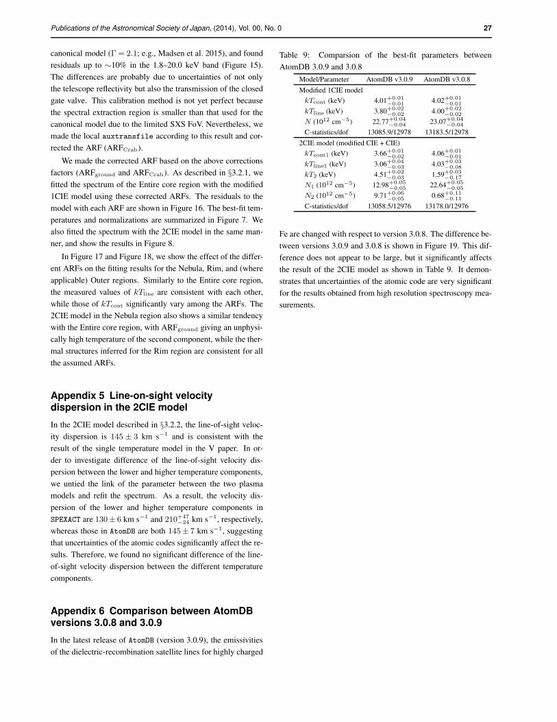
Publications of the Astronomical Society of Japan, (2014), Vol. 00, No. 0 27
canonical model (Γ = 2.1; e.g., Madsen et al. 2015), and found
residuals up to ∼10% in the 1.8–20.0 keV band (Figure 15).
The differences are probably due to uncertainties of not only
the telescope reflectivity but also the transmission of the closed
gate valve. This calibration method is not yet perfect because
the spectral extraction region is smaller than that used for the
canonical model due to the limited SXS FoV. Nevertheless, we
made the local auxtransfile according to this result and cor-
rected the ARF (ARFCrab).
We made the corrected ARF based on the above corrections
factors (ARFground and ARFCrab). As described in §3.2.1, we
fitted the spectrum of the Entire core region with the modified
1CIE model using these corrected ARFs. The residuals to the
model with each ARF are shown in Figure 16. The best-fit tem-
peratures and normalizations are summarized in Figure 7. We
also fitted the spectrum with the 2CIE model in the same man-
ner, and show the results in Figure 8.
In Figure 17 and Figure 18, we show the effect of the differ-
ent ARFs on the fitting results for the Nebula, Rim, and (where
applicable) Outer regions. Similarly to the Entire core region,
the measured values of kTline are consistent with each other,
while those of kTcont significantly vary among the ARFs. The
2CIE model in the Nebula region also shows a similar tendency
with the Entire core region, with ARFground giving an unphysi-
cally high temperature of the second component, while the ther-
mal structures inferred for the Rim region are consistent for all
the assumed ARFs.
Appendix 5 Line-on-sight velocitydispersion in the 2CIE model
In the 2CIE model described in §3.2.2, the line-of-sight veloc-
ity dispersion is 145 ± 3 km s−1 and is consistent with the
result of the single temperature model in the V paper. In or-
der to investigate difference of the line-of-sight velocity dis-
persion between the lower and higher temperature components,
we untied the link of the parameter between the two plasma
models and refit the spectrum. As a result, the velocity dis-
persion of the lower and higher temperature components in
SPEXACT are 130± 6 km s−1 and 210+47−24 km s−1, respectively,
whereas those in AtomDB are both 145± 7 km s−1, suggesting
that uncertainties of the atomic codes significantly affect the re-
sults. Therefore, we found no significant difference of the line-
of-sight velocity dispersion between the different temperature
components.
Appendix 6 Comparison between AtomDBversions 3.0.8 and 3.0.9
In the latest release of AtomDB (version 3.0.9), the emissivities
of the dielectric-recombination satellite lines for highly charged
Table 9: Comparsion of the best-fit parameters between
AtomDB 3.0.9 and 3.0.8
Model/Parameter AtomDB v3.0.9 AtomDB v3.0.8
Modified 1CIE model
kTcont (keV) 4.01+0.01−0.01
4.02+0.01−0.01
kTline (keV) 3.80+0.02−0.02 4.00+0.02
−0.02
N (1012 cm−5) 22.77+0.04−0.04 23.07+0.04
−0.04
C-statistics/dof 13085.9/12978 13183.5/12978
2CIE model (modified CIE + CIE)
kTcont1 (keV) 3.66+0.01−0.02
4.06+0.01−0.01
kTline1 (keV) 3.06+0.04−0.03 4.03+0.03
−0.08
kT2 (keV) 4.51+0.02−0.03 1.59+0.03
−0.17
N1 (1012 cm−5) 12.98+0.05−0.05
22.64+0.05−0.05
N2 (1012 cm−5) 9.71+0.06−0.05
0.68+0.11−0.11
C-statistics/dof 13058.5/12976 13178.0/12976
Fe are changed with respect to version 3.0.8. The difference be-
tween versions 3.0.9 and 3.0.8 is shown in Figure 19. This dif-
ference does not appear to be large, but it significantly affects
the result of the 2CIE model as shown in Table 9. It demon-
strates that uncertainties of the atomic code are very significant
for the results obtained from high resolution spectroscopy mea-
surements.
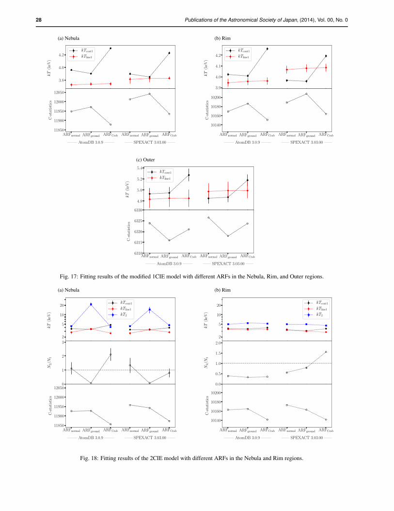
28 Publications of the Astronomical Society of Japan, (2014), Vol. 00, No. 0
(a) Nebula
3.8
4.0
4.2
kT
(keV
)kTcont1
kTline1
ARFnormal ARFground ARFCrab ARFnormal ARFground ARFCrab
11850
11900
11950
12000
12050
C-statistics
——– AtomDB 3.0.9 ——– —— SPEXACT 3.03.00 ——
(b) Rim
3.9
4.0
4.1
4.2
kT
(keV
)
kTcont1
kTline1
ARFnormal ARFground ARFCrab ARFnormal ARFground ARFCrab
10140
10160
10180
10200
C-statistics
——– AtomDB 3.0.9 ——– —— SPEXACT 3.03.00 ——
(c) Outer
4.8
5.0
5.2
5.4
kT
(keV
)
kTcont1
kTline1
ARFnormal ARFground ARFCrab ARFnormal ARFground ARFCrab6310
6315
6320
6325
6330
C-statistics
——– AtomDB 3.0.9 ——– —— SPEXACT 3.03.00 ——
Fig. 17: Fitting results of the modified 1CIE model with different ARFs in the Nebula, Rim, and Outer regions.
(a) Nebula
2
5
10
20
kT
(keV
)
kTcont1
kTline1
kT2
0
1
2
3
N2/N
1
ARFnormal ARFground ARFCrab ARFnormal ARFground ARFCrab
11850
11900
11950
12000
12050
C-statistics
——– AtomDB 3.0.9 ——– —— SPEXACT 3.03.00 ——
(b) Rim
2
5
10
20
kT
(keV
)
kTcont1
kTline1
kT2
0.0
0.5
1.0
1.5
2.0
N2/N
1
ARFnormal ARFground ARFCrab ARFnormal ARFground ARFCrab
10140
10160
10180
10200
C-statistics
——– AtomDB 3.0.9 ——– —— SPEXACT 3.03.00 ——
Fig. 18: Fitting results of the 2CIE model with different ARFs in the Nebula and Rim regions.
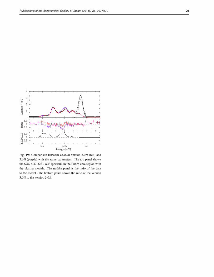
Publications of the Astronomical Society of Japan, (2014), Vol. 00, No. 0 29
1
2
3
4
Cou
nts
s−1
keV
−1
0.81
1.2
Rat
io
6.5 6.55 6.6
0.81
1.2
3.0.
8/3.
0.9
Energy (keV)
Fig. 19: Comparison between AtomDB version 3.0.9 (red) and
3.0.8 (purple) with the same parameters. The top panel shows
the SXS 6.47–6.63 keV spectrum in the Entire core region with
the plasma models. The middle panel is the ratio of the data
to the model. The bottom panel shows the ratio of the version
3.0.8 to the version 3.0.9.