Temperature Compensation through Systems Biology

Peter Ruoff 1 *, Maxim Zakhartsev2# and Hans V. Westerhoff3

1Department of Mathematics and Natural Science, University of Stavanger, N-4036

Stavanger, Norway, 2Biochemical Engineering, International University of Bremen,

Campus Ring 1, D-28759 Bremen, Germany, EU, 3Manchester Centre for Integrative

Systems Biology, School for Chemical Engineering and Analytical Sciences, The

University of Manchester, Manchester M601QD, UK, EU and BioCentrumAmsterdam, BioCentre Amsterdam, FALW, Free University, NL-1081 HV Amsterdam,The Netherlands, EU.

Running title:Temperature Compensation of Fluxes

Subdivision:Systems biology

*Corresponding author:P. Ruoff, Department of Mathematics and Natural Science, Faculty of Science and

Technology, University of Stavanger, N-4036 Stavanger, Norway. Email:

peter.ruoff@uis.no; fax: (+47) 51841750; url: http://www.ux.uis.no/~ruoff

Keywords:Temperature compensation, gene expression, metabolic regulation, control

coefficients, systems biology

#present address: Department of Marine Animal Physiology, Alfred Wegener Institute

for Marine and Polar Research (AWI), Building E, office 1555, Am Handelshaven 12,D-27570 Bremerhaven, Germany.

- 2 -

Summary

Temperature has a strong influence on most individual biochemical reactions.

Despite this, many organisms have the remarkable ability to keep certain physiological

fluxes approximately constant over an extended temperature range. In this paper it is

shown how temperature compensation can be considered as a pathway phenomenon

rather than the result of a single-enzyme property. By using metabolic control analysis

reaction networks that exhibit temperature compensation can be identified. Because

most activation enthalpies are positive, temperature compensation of a flux can occur

when certain control coefficients are negative. This can be achieved in networks with

branching reactions or if the first irreversible reaction is regulated by a feedback loop.

Hierarchical control analysis shows that networks that are dynamic through regulated

gene expression or signal transduction may offer additional possibilities to bring the

apparent activation enthalpies close to zero and leading to temperature compensation.

A calorimetric experiment with yeast provides evidence that such a dynamic

temperature adaptation can actually occur.

Introduction

Temperature is an environmental factor, which influences most of the

chemical processes occurring in living and nonliving systems. Van’t Hoff’s rule states

that reaction rates increase by a factor (the Q10) of two or more when the temperature

is increased by ten centigrades [1]. Despite this strong influence of temperature on

individual reactions, many organisms have the remarkable ability to keep some of

their metabolic fluxes at an approximately constant level over an extended

temperature range. Examples are the oxygen consumption rates of ectoterms living in

costal zones [2] and of fish [3], the period lengths of all circadian [4] and some

- 3 -

ultradian [5, 6] rhythms, photosynthesis in cold adapted plants [7, 8], homeostasis

during fever [9], or the regulation of heat shock proteins [10].

In 1957 Hastings and Sweeney suggested that in biological clocks such

temperature compensation may occur as the result of opposing reactions within the

metabolic network [11]. A later kinetic analysis of the problem [12] came essentially

to the same conclusion, and predictions of the theory were recently tested by

experiments using Neurospora’s circadian clock [13] and chemical oscillators [14,

15].

In this paper we use metabolic and hierarchical control analysis [16-22] to

show how certain steady state fluxes in static reaction networks can be temperature

compensated according to a similar principle and how dynamic networks have an

additional repertoire of mechanisms. The content of this paper is mostly theoretical,

but we use the temperature adaptation of yeast cells and the temperature adaptation of

photosynthesis as illustrations. These and other systems (for example adaptation of

gene expression) warrant experimental studies in their own right, which we wish to

cover in subsequent work.

Results and Discussion

Global Condition for Temperature Compensated Flux

In this section the condition for temperature compensation for a global

reaction kinetic network is derived. We refer to this condition as global, because the

network is assumed to contain all biochemical processes (at the genetic and metabolic

levels) that occur in the system. Consider a set of N elementary single step reactions

describing a global network. Each reaction i is assigned a rate constant ki [23] and a

steady state flux (reaction rate) Ji with associated activation enthalpy

€

Eaki . Here

- 4 -

reversible reactions may be considered as two separate reactions; an alternative is to

look upon ki as a parameter that proportionally affects both the forward and the

reverse reaction of the step [23]. Rate constants and absolute temperature are

connected through the Arrhenius equation

€

ki = Aie−Eaki

RT , where activation enthalpies

€

Eaki are considered to be independent of temperature. The Arrhenius factor Ai

subsumes any structural activation entropy. Flux Jj (i.e., the flux of elementary

reaction “j”) becomes temperature compensated within a temperature interval around

a reference temperature Tref (at which parameters and rate constants are defined) if the

following balancing equation is satisfied (for derivation, see Supplementary Material):

€

d lnJ j

d lnT=1RT

*CiJ j Ea

ki = 0i=1

N

∑ (1a)

€

*CiJ j is the global control coefficient [19, 21] of flux with respect to the rate constant

ki defined as

€

*CiJ j =

∂ lnJ j

∂ lnki.

€

*CiJ j measures the change in flux for a fractional increase

in ki, therein comprising the effects of changes in gene expression or signal

transduction that may affect the concentration and activity of the enzyme catalyzing

step. In general, the global control coefficients obey the summation theorem

€

*CiJ j =1

i=1

N

∑ [19, 21]. Because the activation enthalpies (

€

Eaki ) are positive, temperature

compensation is only possible if some of the global control coefficients are negative.

The condition for temperature compensation using metabolic control coefficients

Sometimes a biochemical system is described only at its metabolic level of

organization. In this case, one can use metabolic control coefficients denoted by

capital C without the asterisk [19, 21], which is a set addressing the control by all the

- 5 -

enzymes/steps at the metabolic level and do not include transcriptional, translational

processes or signal transduction events. The effects of these at the metabolic level

should be made explicit in terms of changes in amount or covalent modification state

of the enzymes. Accordingly, the ‘balancing equation’ is given by (see Supplementary

Material for derivation):

€

d lnJ j

d lnT= Cki

catJ j Ea

kicat

RT+ Ckm

catJ j RT

em

m∑ +

i∑ RKl

J j

l∑ Ea

Kl

RT= 0 (1b)

The first term on the right-hand side of Eq. 1b describes the contribution of

€

kicat

(turnover number), where

€

CkicatJ j =

∂ lnJ j

∂ lnkicat is the metabolic control coefficient and

€

Eakicat

is the corresponding activation enthalpy of the turnover number

€

kicat . The second term

is the contribution due to the variation of the concentration of active enzyme m (em)

by altered gene expression, translation, or signal transduction. It contains the

temperature response coefficient of the activity of that step

€

RTem ≡

d lnemd lnT

. If one is not

aware of the change in enzyme activity due to these hierarchical mechanisms, one

may measure an apparent activation enthalpy

€

Ea,apparentkicat

= Eakicat

+ RT ⋅ RTei . With this

Eq. 1b reduces to:

€

d lnJ j

d lnT= Cki

catJ j Ea,apparent

kicat

RT+

i∑ RKl

J j

l∑ Ea

Kl

RT= 0 (1c)

If an increase in temperature leads to a decreased expression level of the enzyme

catalyzing step m, the temperature response coefficient of the enzyme becomes

negative. The apparent activation enthalpy of that step in a metabolic network may

have zero or negative values.

The final term in Eq. 1b describes the contribution due to changes in the rapid

equilibria or steady states that the enzyme is engaged in with substrates, inhibitors,

- 6 -

and activators. For substrates Xl , Kl is the (apparent) Michaelis constant and

€

EaKl is

the formation enthalpy

€

ΔHl0 associated with Kl [1, 24].

€

EaKl tends to be positive in

sign, favoring dissociation at higher temperatures [1, 24].

€

RKl

J j =∂ lnJ j∂ lnKl

is the

response coefficient of the flux with respect to an increase in the Michaelis constant

[25].

An example of temperature compensation through and of an enzyme’s

expression level

In the following example we illustrate the usage of global and metabolic

control coefficients to get temperature compensation in a enzyme’s activity and steady

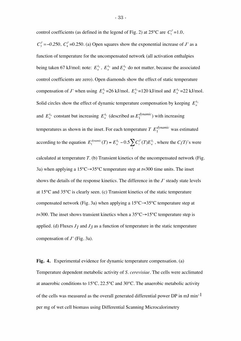
state level. Fig. 1 shows a model of an enzyme’s expression (translation and

transcription), where the enzyme catalyzes the reaction S → P. For the sake of

simplicity, we assume that transcription, translation and the degradation processes

have pseudo first-order kinetics with respect to their substrates, i.e. we neglect

saturation effects for the RNA polymerase catalyzing transcription, the RNase

catalyzing the breakdown of RNA, the ribosomes catalyzing the synthesis of E, and

the proteasomes/proteases catalyzing the degradation of E. The steady state flux (J5)

through step 5 for producing P is described by

€

J5 =k5catess[S]KM + [S]

=k1k3k5

cat

k2k4⋅

[S]KM + [S]

(2)

where ess is the steady state level of E, i.e. the level attained after all processes in the

system have relaxed, including those of transcription and translation. The global

control coefficients calculated from this equation are

€

*Ck5catJ5 =1 and

€

*CkiJ5 =1 for i=1, 3

and −1 for i=2, 4 while the (global) response coefficient with respect to the Michaelis

- 7 -

constant amounts to

€

*RKM

J5 =∂ lnJ5∂ lnKM

−KM

KM + [S]. Assuming an Arrhenius temperature

dependence of rate constants ki and

€

k5cat , J5 can be temperature compensated due to

the negative control coefficients of reactions 2 and 4. If the enthalpy of formation of

the enzyme substrate complex is negative (which is the more common case), such

compensation may also derive from the negative response coefficient.

Likewise, when describing the system at the metabolic level we get

€

Ck5catJ5 =1

and the (metabolic) response coefficient

€

RKM

J5 =∂ lnJ5∂ lnKM

−KM

KM + [S]. Because

€

d lnJ5dT

and the activation and formation enthalpies are unaffected whether the description

occurs globally or at a metabolic level, an expression for the temperature variation of

the enzyme’s steady state level can be found by comparing the global and metabolic

balancing equations (Eqs. 1a, 1b)

€

Ea,apparentk5cat

− Eak5cat

RT=d lnessd lnT

=1RT(Ea

k1 + Eak3 − Ea

k2 − Eak4 ) (3)

showing that ess can become temperature compensated when the sum of activation

enthalpies in Eq. 3 becomes zero.

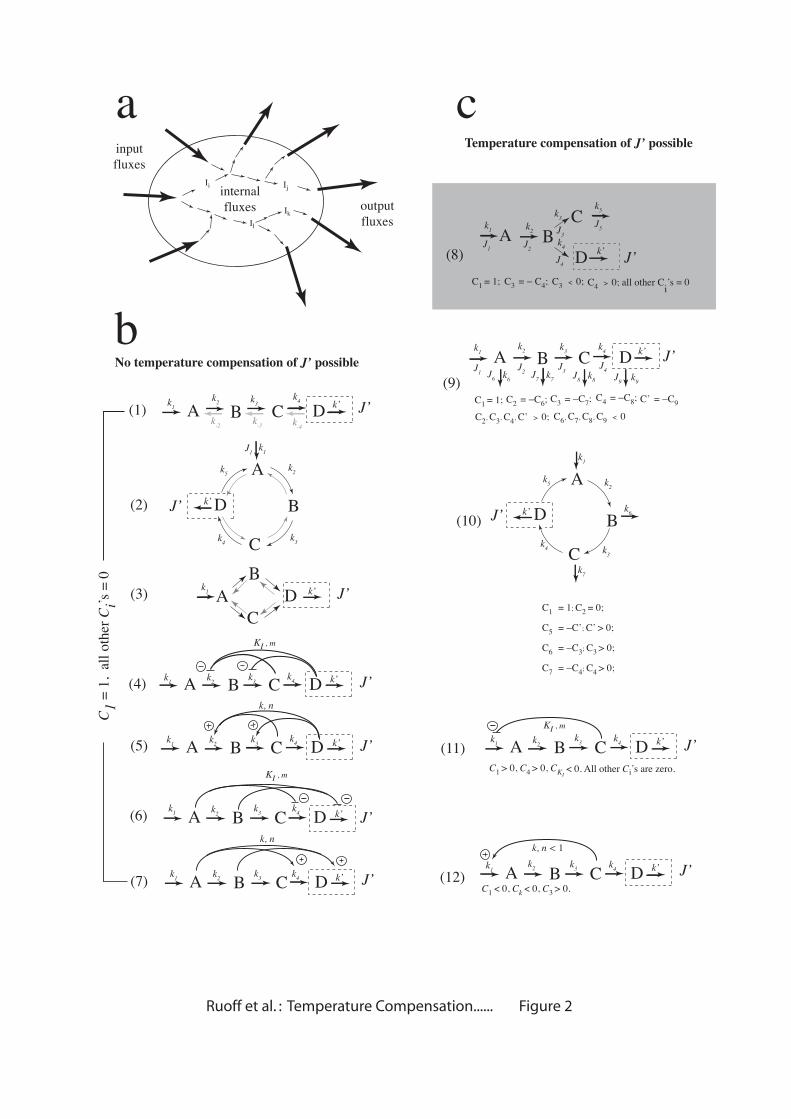
Rules for temperature compensated and uncompensated flux in fixed networks

We now investigate the conditions for temperature compensation in simple

reaction networks. The fluxes (reaction rates) can be characterized as input, internal,

and output fluxes (Fig. 2a). Under what conditions can a certain (output) flux (say J’)

become temperature compensated? In order to keep such an analysis tractable the

number of reaction intermediates are limited to four. In addition, input fluxes were

limited to one with one or several output fluxes. An overview of the networks is

shown in Figs. 2b and 2c. It may be noted that these networks do not represent a

- 8 -

complete set of all possible networks containing four intermediates, but represent

examples for which temperature compensation of flux J’ becomes possible or not.

However, based on these networks it is possible to derive some general rules (see

below). For the sake of simplicity we assume that the considered networks consist of

first-order reactions (except when including feedback loops). In a metabolic context,

this would reflect the view that under physiological conditions the enzymes which

catalyze each reaction step are not saturated by their substrates [26]. Positive

feedforward or feedback loops from an intermediate I to process i are described by

substituting the original rate constant ki with kik[I]n, where k is an activation constant

and n is the cooperativity (Hill coefficient). Negative feedback or feedforward loops

from intermediate I to process i are described by substituting ki with ki/(KI+[I]m),

where KI is an inhibitor constant and m is the cooperativity. For each network the

steady state output flux J’ (indicated by the dashed box in each scheme) is examined

in terms of whether temperature compensation is possible. The tested networks (see

Supplementary Material) were then divided into those where J’ is unable to exhibit

temperature compensation (Fig. 2b) and those where J’ can be compensated (Fig. 2c).

The following rules can be stated. Temperature compensation of an output

flux is not possible for (i) any (reversible or irreversible) chain or loop of (first-order)

reactions or a branched network which has only one output flux and a product

insensitive first step (Fig. 2b, schemes (1)-(3)); (ii) networks with only one output flux

having in addition positive and/or negative feedback loops which are assigned to

internal fluxes or to an output flux, but not to the first step (Fig. 2b schemes (4)-(7)).

In all schemes of Fig. 2b we have that C1=1, while all the other control coefficients

are zero. Temperature compensation of an output flux becomes possible when (i) the

network has more than one output flux (Fig. 2c, schemes (8)-(10)) or (ii) the networks

- 9 -

have positive and/or negative feedback loops which are assigned to at least one input

flux (Fig. 2c, schemes (11)-(12)).

From static to dynamic temperature compensation

In the derivation of Eqs. 1a and 1b we assumed that activation enthalpies are

constants and independent of temperature. While this assumption is realistic for

single-step elementary reactions, at the metabolic level of description activation

enthalpies of enzyme catalyzing steps may depend on temperature as enzymes may be

affected by temperature dependent processes such as phosphorylation,

dephosphorylation, conformational changes, etc. Due to these different levels of

description we distinguish between static and dynamic temperature compensation. By

static temperature compensation we mean that all activation enthalpies are assumed to

be temperature independent and constant, and together fulfill the balancing equation

for a certain reference temperature. To illustrate static and dynamic temperature

compensation as well as uncompensated behavior we use scheme 8 (Fig. 2c) as an

example. This scheme is one of the simplest models that can show temperature

compensation of output flux J’. The control coefficients can be easily calculated (see

Supplementary Material). We have taken a set of arbitrary chosen rate constant

values, and it may be noted that the behavior shown below are not specific for the

chosen rate constant values. Similar behavior can be obtained with any set of rate

constants. Independent of the chosen rate constant values uncompensated behavior is

obtained when all activation enthalpies are chosen to be equal, for example

€

Ea' . In

this case, using the summation theorem

€

*CiJ ' =1

i=1

N

∑ , Eq. 1a can be expressed as

€

d lnJ 'd lnT

=Ea'

RT, showing that flux J’ is highly dependent on temperature. Such

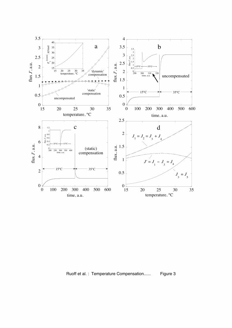
- 10 -

uncompensated behavior is shown in Fig. 3a (open squares) when all activation

enthalpies in scheme (8) (Fig. 2c) are set to 67 kJ/mol. In this case J’ shows an

exponential increase with temperature. In Fig. 3b the increase in J’ is seen when a

15°C → 35°C temperature step is applied to the uncompensated system. In static

temperature compensation the activation enthalpies have been chosen such that Eq. 1a

is approximately fulfilled at Tref (25°C) at which the rate constants have been defined

and the control coefficients have been evaluated (open diamonds, Fig. 3a). The

condition for static temperature compensation of scheme (8) reads:

€

Eak1 + C4

J ' (Eak4 − Ea

k3 ) ≅ 0 with

€

C4J ' =

k3k3 + k4

(see Supplementary Material). Because

the control coefficients depend on the rate constants and therefore also on

temperature, the static compensated flux J’ will gradually change over an extended

temperature range as shown in Fig. 3a.

In dynamic compensation, one (or several) of the apparent (see above) or real

activation enthalpies is allowed to change as a function of temperature. Processes that

may lead to this include posttranslational processing of proteins such as

phosphorylation, dephosphorylation, or conformational changes, splice variation, etc.

[27, 28]. For example, when

€

Eak1 increases with temperature as shown in the inset of

Fig. 3a, J’ becomes practically independent of temperature (solid circles, Fig. 3a).

Incidentally, temperature compensation means that a steady state flux (or the

period length of an oscillatory flux, as for example in circadian rhythms) is (virtually)

the same at different but constant temperatures. However, when a sudden change in

temperature is applied, either as a step or as a pulse, even in temperature compensated

systems transient kinetics are observed as illustrated in Fig. 3c. By applying a

temperature step, J’ undergoes an excursion and relaxes back to its steady state. The

time scale of relaxation will be dependent on the rate constants, i.e., metabolic

- 11 -

relaxation typically occurs in the subminute range. When gene expression adaptation

is involved, relaxation may be much slower.

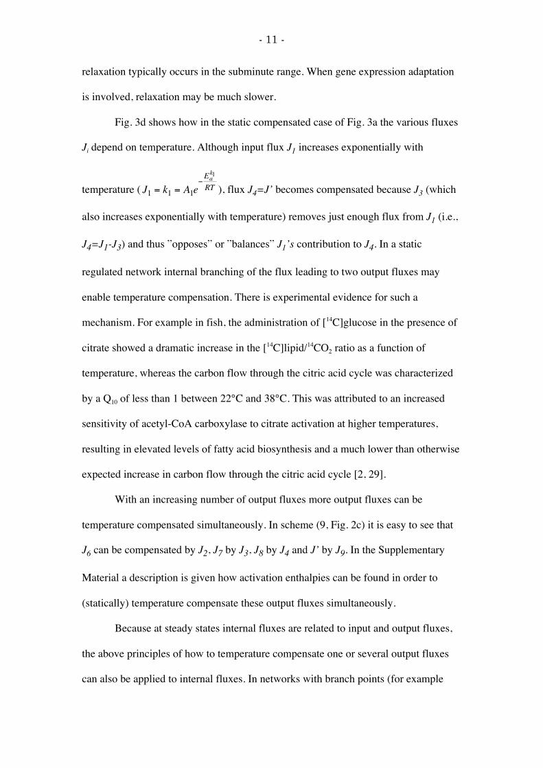
Fig. 3d shows how in the static compensated case of Fig. 3a the various fluxes

Ji depend on temperature. Although input flux J1 increases exponentially with

temperature (

€

J1 = k1 = A1e−Eak1

RT ), flux J4=J’ becomes compensated because J3 (which

also increases exponentially with temperature) removes just enough flux from J1 (i.e.,

J4=J1-J3) and thus ”opposes” or ”balances” J1’s contribution to J4. In a static

regulated network internal branching of the flux leading to two output fluxes may

enable temperature compensation. There is experimental evidence for such a

mechanism. For example in fish, the administration of [14C]glucose in the presence of

citrate showed a dramatic increase in the [14C]lipid/14CO2 ratio as a function of

temperature, whereas the carbon flow through the citric acid cycle was characterized

by a Q10 of less than 1 between 22°C and 38°C. This was attributed to an increased

sensitivity of acetyl-CoA carboxylase to citrate activation at higher temperatures,

resulting in elevated levels of fatty acid biosynthesis and a much lower than otherwise

expected increase in carbon flow through the citric acid cycle [2, 29].

With an increasing number of output fluxes more output fluxes can be

temperature compensated simultaneously. In scheme (9, Fig. 2c) it is easy to see that

J6 can be compensated by J2, J7 by J3, J8 by J4 and J’ by J9. In the Supplementary

Material a description is given how activation enthalpies can be found in order to

(statically) temperature compensate these output fluxes simultaneously.

Because at steady states internal fluxes are related to input and output fluxes,

the above principles of how to temperature compensate one or several output fluxes

can also be applied to internal fluxes. In networks with branch points (for example

- 12 -

scheme (8, Fig. 2c)), at least one of the downstream internal fluxes after the branch

point can be temperature compensated, while none of the upstream fluxes can show

temperature compensation unless there are more branch points upstream. The same

applies also to cyclic networks. Testing for example the irreversible clockwise scheme

(2, Fig. 2b), fluxes J2, J3, J4 and J5 can be temperature compensated while J1 and J’

cannot show temperature compensation.

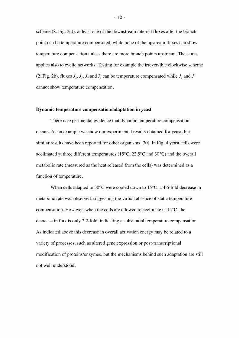
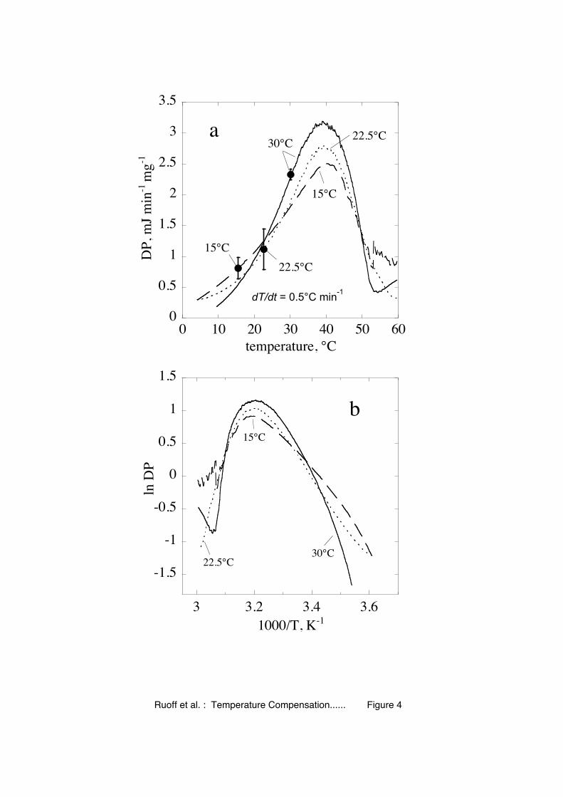
Dynamic temperature compensation/adaptation in yeast

There is experimental evidence that dynamic temperature compensation

occurs. As an example we show our experimental results obtained for yeast, but

similar results have been reported for other organisms [30]. In Fig. 4 yeast cells were

acclimated at three different temperatures (15°C, 22.5°C and 30°C) and the overall

metabolic rate (measured as the heat released from the cells) was determined as a

function of temperature.

When cells adapted to 30°C were cooled down to 15°C, a 4.6-fold decrease in

metabolic rate was observed, suggesting the virtual absence of static temperature

compensation. However, when the cells are allowed to acclimate at 15°C, the

decrease in flux is only 2.2-fold, indicating a substantial temperature compensation.

As indicated above this decrease in overall activation energy may be related to a

variety of processes, such as altered gene expression or post-transcriptional

modification of proteins/enzymes, but the mechanisms behind such adaptation are still

not well understood.

- 13 -

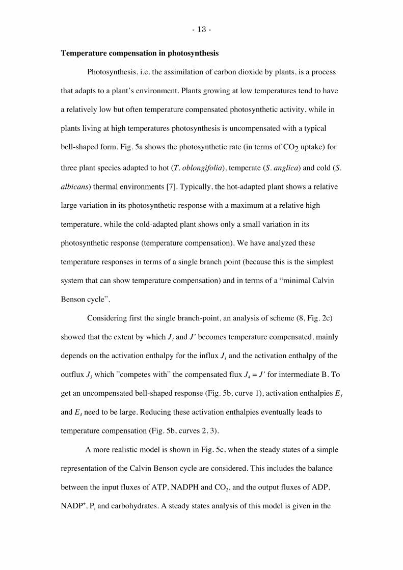
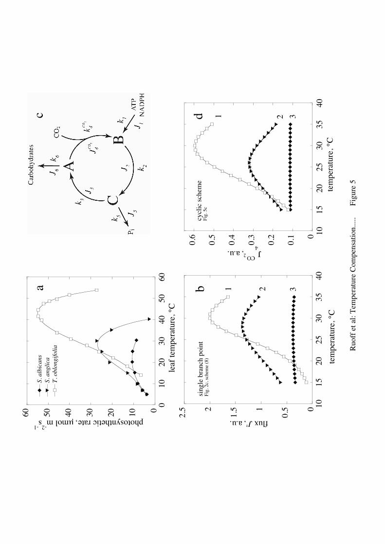
Temperature compensation in photosynthesis

Photosynthesis, i.e. the assimilation of carbon dioxide by plants, is a process

that adapts to a plant’s environment. Plants growing at low temperatures tend to have

a relatively low but often temperature compensated photosynthetic activity, while in

plants living at high temperatures photosynthesis is uncompensated with a typical

bell-shaped form. Fig. 5a shows the photosynthetic rate (in terms of CO2 uptake) for

three plant species adapted to hot (T. oblongifolia), temperate (S. anglica) and cold (S.

albicans) thermal environments [7]. Typically, the hot-adapted plant shows a relative

large variation in its photosynthetic response with a maximum at a relative high

temperature, while the cold-adapted plant shows only a small variation in its

photosynthetic response (temperature compensation). We have analyzed these

temperature responses in terms of a single branch point (because this is the simplest

system that can show temperature compensation) and in terms of a “minimal Calvin

Benson cycle”.

Considering first the single branch-point, an analysis of scheme (8, Fig. 2c)

showed that the extent by which J4 and J’ becomes temperature compensated, mainly

depends on the activation enthalpy for the influx J1 and the activation enthalpy of the

outflux J3 which ”competes with” the compensated flux J4 = J’ for intermediate B. To

get an uncompensated bell-shaped response (Fig. 5b, curve 1), activation enthalpies E3

and E4 need to be large. Reducing these activation enthalpies eventually leads to

temperature compensation (Fig. 5b, curves 2, 3).

A more realistic model is shown in Fig. 5c, when the steady states of a simple

representation of the Calvin Benson cycle are considered. This includes the balance

between the input fluxes of ATP, NADPH and CO2, and the output fluxes of ADP,

NADP+, Pi and carbohydrates. A steady states analysis of this model is given in the

- 14 -

Supplementary Material section showing that the assimilation of CO2 (

€

J4CO2 ) can be

temperature compensated, because of the balance of fluxes J1, J3, J4 (positive

contributions) with fluxes J5 and J6 (negative contributions). When the activation

enthalpies of J1 and J3 dominate

€

J4CO2 shows the bell-shaped response for hot-adapted

species (curve 1, Fig. 5d). Temperature compensation can be achieved when the

positive contributions balance the negative, i.e., when the activation enthalpies of J1

and J3 are reduced (curve 3, Fig. 5d).

Conclusion

In this paper we have derived a general relationship how temperature

compensation of biochemical steady state flux can occur by means of the balancing

equations (1a-c). Our focus here was primarily how dynamic temperature

compensation can occur through systems biology mechanisms [31]. The analysis

shows that certain network topologies need to be met in order to get negative control

coefficients. These negative control coefficients oppose the overall positive

contributions of the control coefficients as indicated by the summation theorem

€

*CiJ j

i=1

N

∑ =1 (or

€

CkicatJ j

i∑ =1 at the metabolic level). This can be achieved by various

means: positive and negative feedforward and/or feedback loops, signal transduction

events (for example by phosphorylation, dephosphorylation) and by adaptation

through gene expression. As a special case of the derived principle temperature

compensation can occur for a single enzyme (”instantaneous temperature

compensation” [2]) when balancing occurs for example between the enzyme’s

Michaelis constant (KM, KD) and its turnover number [32]. In this case, mechanisms

which include enzyme-substrate interactions, enzyme modulator interactions,

- 15 -

metabolic branch points, or conformational changes [2, 27, 28] may be involved.

While quantum mechanical tunneling is principally temperature independent, studies

with methylamine dehydrogenase showed a strong temperature dependence of the

enzyme catalyzed process where thermal activation or “breathing” of the protein

molecule is required to facilitate the tunneling reaction [33].

A challenge in applying realistic models will be the description of how

apparent activation enthalpies change with temperature and of the actual mechanisms

involved in these processes.

Materials and Methods

Determination of Yeast Metabolic Activities. The wild type yeast strain

Saccharomyces cereviciae SPY509 (from the European Saccharomyces cerevisiae

Archive of Functional Analysis (EUROSCARF, http://web.uni-

frankfurt.de/fb15/mikro/euroscarf/) with genotype MAT or a, his3_1, leu2_0, lys2_0,

ura3_0 were grown in 250 ml flasks in 100 ml of complex YPD media (10 g yeast

extract, 20 g peptone, and 20 g glucose in 1000 ml of the media) under constant

nitrogen bubbling through the media and agitated with 250 rpm at various acclimation

temperatures [34, 35]. Yeast cultures were always kept at early exponential growth

phase (OD660 < 2) by diluting the culture with fresh media at each particular

temperature. The acclimation time was for at least 10-14 days. A differential scanning

calorimeter (VP-DSC, MicroCal, USA) was used for measurements of heat

production by living yeast. The yeast cells were washed in a 100 mM glucose solution

(pH 5.5) at the relevant acclimation temperature under nitrogen bubbling so as to

remove the YPD media, which has a high specific heat capacity, resuspended in 100

mM glucose solution to 10 g wet cell biomass per liter, and incubated at the

- 16 -

acclimation temperature under a nitrogen atmosphere for 1 hour before the

measurements.

Before the measurements all solutions were degassed, including the

suspension of living cells. 100 mM glucose solution was used as the reference for the

differential scanning calorimeter (DSC) measurements. The heat production was

determined between 4°C and 60° using a scanning rate of 0.5°C min-1. Two

independent sets of cells were scanned starting from the acclimation temperature

either down to 4°C or up to 60°. The heat production has been expressed in units of

differential power (DP) per mg of wet cell biomass (mJ min-1 mg-1). After each

measurement the yeast suspension was replaced with a freshly prepared one. About

80% of the metabolic activity of the yeast cells was estimated to correspond to

anaerobic glycolysis.

Model Calculations. Numerical calculations were performed using the FORTRAN

subroutine LSODE (Livermore Solver of Ordinary Differential Equations) [36]. Some

analytical solutions of steady state fluxes were obtained with the help of MATLAB

(www.mathworks.com).

Abbreviations and Symbols

Ci abbreviation used in Supplementary Material for

€

∂ lnJ '∂ lnki

=kiJ'

∂J'∂ki

.

€

*CiJ j global control coefficient defined as

€

∂ lnJ j

∂ lnki=kiJ j

∂J j

∂ki

.

€

CkicatJ j metabolic control coefficient defined as

€

∂ lnJ j

∂ lnkicat =

kicat

J j

∂J j

∂kicat

.

ei concentration of enzyme catalyzing process i.

- 17 -

ess steady state concentration of enzyme E in Fig. 1; see also Eq. 3.

Ei abbreviation used in Supplementary Material for

€

Eaki .

€

Eaki activation enthalpy of elementary component process with rate constant ki.

€

Eaki and ki are related by the Arrhenius equation

€

ki = Aie−Eaki

RT .

€

Eakicat

activation enthalpy of turnover number

€

kicat of enzyme catalyzed process i.

€

EaKi is the formation enthalpy

€

ΔHi0 of the rapid equilibrium between enzyme and

substrate in enzyme catalyzed process i. The temperature dependence of Ki(or other equilibrium constants such as KM, KI) is analogous to the Arrhenius

equation, i.e.,

€

Ki = eΔSi

0

R e−ΔHi

0

RT .

Jj, flux (reaction rate) of elementary component process j, or flux of enzymecatalyzed process j.

k activation constant used in positive feedforward/feedback loop.

ki rate constant of elementary component process i.

€

kicat turnover number of enzyme catalyzed process i.

Ki rapid equilibrium (dissociation) constant between enzyme and substrate inenzyme catalyzed process i.

KI inhibition constant used in negative feedforward/feedback loop. For itstemperature dependence see also above description of

€

EaKi and description of

scheme (11) in Supplementary Material.

KM Michaelis constant (Fig. 1).

m Used as an index for enzyme-catalyzed processes or used to describe thecooperativity (Hill coefficient) in negative feedforward/feedback loops actingfrom intermediate I on reaction i by replacing ki with ki/(KI+[I]m).

n Cooperativity (Hill coefficient) in positive feedforward/feedback loops actingfrom intermediate I on reaction i by replacing ki with kik[I]n.

R gas constant.

€

RTem metabolic response coefficient defined as

€

d lnemd lnT

.

- 18 -

€

RKi

J j metabolic response coefficient defined as

€

d lnJ j

d lnKi

.

€

*RKi

J j global response coefficient defined as

€

d lnJ j

d lnKi

.

T temperature.

Tref reference temperature at which rate constants and parameters are defined.

- 19 -

References1. Laidler, K. J. & Meiser, J. H. (1995) Physical Chemistry. Second Edition,

Houghton Mifflin Company, Geneva (Illinois).2. Hazel, J. R. & Prosser, C. L. (1974) Molecular Mechanisms of Temperature

Compensation in Poikilotherms, Physiol Rev. 54, 620-677.3. Zakhartsev, M. V., De Wachter, B., Sartoris, F. J., Portner, H. O. & Blust, R.

(2003) Thermal physiology of the common eelpout (Zoarces viviparus), J Comp

Physiol [B]. 173, 365-78.4. Bünning, E. (1963) The Physiological Clock, Springer-Verlag, Berlin.

5. Lloyd, D. & Murray, D. B. (2005) Ultradian metronome: timekeeper for

orchestration of cellular coherence, Trends Biochem Sci. 30, 373-7.6. Iwasaki, K., Liu, D. W. & Thomas, J. H. (1995) Genes that control a temperature-

compensated ultradian clock in Caenorhabditis elegans, Proc Natl Acad Sci U S A. 92,10317-21.

7. Baker, N. R., Long, S. P. & Ort, D. R. (1988) Photosynthesis and temperature,

with particular reference to effects on quantum yield, Symp Soc Exp Biol. 42, 347-75.8. Cabrera, H. M., Rada, F. & Cavieres, L. (1998) Effects of temperature on

photosynthesis of two morphologically contrasting plant species along an altitudinalgradient in the tropical high Andes, Oecologia. 114, 145-152.

9. Pollheimer, J., Zellner, M., Eliasen, M. M., Roth, E. & Oehler, R. (2005) Increased

susceptibility of glutamine-depleted monocytes to fever-range hyperthermia: the roleof 70-kDa heat shock protein, Ann Surg. 241, 349-55.

10. Peper, A., Grimbergen, C. A., Spaan, J. A., Souren, J. E. & van Wijk, R. (1998)A mathematical model of the hsp70 regulation in the cell, Int J Hyperthermia. 14, 97-

124.

11. Hastings, J. W. & Sweeney, B. M. (1957) On the mechanism of temperatureindependence in a biological clock, Proc Natl Acad Sci U S A. 43, 804-811.

12. Ruoff, P. (1992) Introducing temperature-compensation in any reaction kineticoscillator model, J Interdiscipl Cycle Res. 23, 92-99.

13. Ruoff, P., Loros, J. J. & Dunlap, J. C. (2005) The relationship between FRQ-

protein stability and temperature compensation in the Neurospora circadian clock,Proc Natl Acad Sci U S A. 102, 17681-6.

14. Kovács, K., Hussami, L. L. & Rábai, G. (2005) Temperature Compensation in the

Oscillatory Bray Reaction, J Phys Chem A. 109, 10302-10306.

- 20 -

15. Kóvacs, K. M., Rábai, G. (2002) Temperature-compensation in pH-oscillators,

Phys Chem Chem Phys. 4, 5265-5269.16. Fell, D. (1997) Understanding the Control of Metabolism, Portland Press,

London and Miami.17. Heinrich, R. & Schuster, S. (1996) The Regulation of Cellular Systems, Chapman

and Hall, New York.

18. Kacser, H. & Burns, J. A. (1973) The control of flux, Symp Soc Exp Biol. 27, 65-104.

19. Kahn, D. & Westerhoff, H. V. (1991) Control theory of regulatory cascades, JTheor Biol. 153, 255-85.

20. Kell, D. & Westerhoff, H. (1986) Metabolic Control Theory: its role in

microbiology and biotechnology, FEMS Microbiol Rev. 39, 305-320.21. Westerhoff, H. V., Koster, J. G., Van Workum, M. & Rudd, K. E. (1990) On the

Control of Gene Expression in Control of Metabolic Processes (Cornish-Bowden, A.,

ed) pp. 399-412, Plenum, New York.22. Cornish-Bowden, A. (2004) Fundamentals of Enzyme Kinetics. Third Edition,

Portland Press, London.23. Brown, G. C., Westerhoff, H. V. & Kholodenko, B. N. (1996) Molecular control

analysis: control within proteins and molecular processes, J Theor Biol. 182, 389-96.

24. Ruoff, P., Christensen, M. K., Wolf, J. & Heinrich, R. (2003) Temperaturedependency and temperature-compensation in a model of yeast glycolytic oscillations,

Biophys Chem. 106, 179-192.25. Chen, Y. & Westerhoff, H. V. (1986) How do Inhibitors and Modifiers of

Individual Enzymes affect steady-state Fluxes and Concentrations in Metabolic

Systems?, Math Modell. 7, 1173-1180.26. Dixon, M., Webb, E. C., Thorne, C. J. R. & Tipton, K. F. (1979) Enzymes,

Longman, London.27. Hochachka, P. W. & Somero, G. N. (2002) Biochemical Adaptation. Mechanism

and Process in Physiological Evolution, Oxford University Press, Oxford.

28. Somero, G. N. (1995) Proteins and temperature, Annu Rev Physiol. 57, 43-68.29. Hochachka, P. W. (1968) Action of temperature on branch points in glucose and

acetate metabolism, Comp Biochem Physiol. 25, 107-18.

- 21 -

30. Hikosaka, K., Ishikawa, K., Borjigidai, A., Muller, O. & Onoda, Y. (2006)

Temperature acclimation of photosynthesis: mechanisms involved in the changes intemperature dependence of photosynthetic rate, J Exp Botany. 57, 291-302.

31. Alberghina, L. & Westerhoff, H. V. (2006) Systems Biology. Definitions and

Perspectives, Springer-Verlag, Berlin.

32. Andjus, R. K., Dzakula, Z., Marjanovic, M. & Zivadinovic, D. (2002) Kinetic

properties of the enzyme-substrate system: a basis for immediate temperaturecompensation, J Theor Biol. 217, 33-46.

33. Sutcliffe, M. J. & Scrutton, N. S. (2000) Enzyme catalysis: over-the-barrier orthrough-the-barrier?, Trends Biochem Sci. 25, 405-8.

34. Burke, D., Dawson, D. & Stearns, T. (2000) Methods in Yeast Genetics. A Cold

Spring Harbor Laboratory Course Manual., Cold Spring Harbor Laboratory Press,Cold Spring Harbor, New York.

35. Sambrook, J., Fritsch, E. F. & Maniatis, T. (1989) Molecular Cloning: A

Laboratory Manual, Cold Spring Harbor Laboratory Press, Cold Spring Harbor, NewYork.

36. Radhakrishnan, K. & Hindmarsh, A. C. (1993) Description and Use of LSODE,

the Livermore Solver for Ordinary Differential Equations. NASA Reference

Publication 1327, Lawrence Livermore National Laboratory Report UCRL-ID-

113855., National Aeronautics and Space Administration, Lewis Research Center,Cleveland, OH 44135-3191.

37. Horton, H. R., Moran, L. A., Scrimgeour, K. G., Perry, M. D. & D., R. J. (2006)Principles of Biochemistry, Pearson Prentice Hall, Upper Saddle River, New Jersey.

- 22 -

Supplementary Material

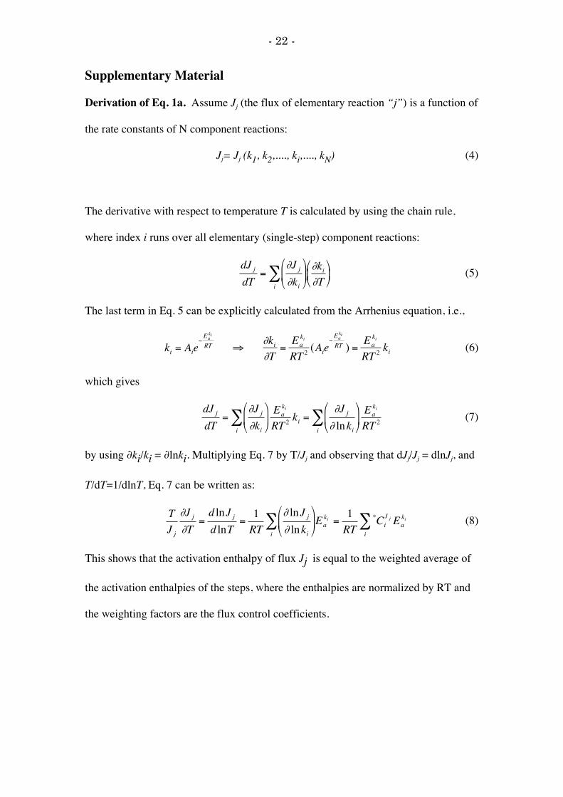
Derivation of Eq. 1a. Assume Jj (the flux of elementary reaction “j”) is a function of

the rate constants of N component reactions:

Jj= Jj (k1, k2,...., ki,...., kN) (4)

The derivative with respect to temperature T is calculated by using the chain rule,

where index i runs over all elementary (single-step) component reactions:

€

dJ j

dT=

∂J j

∂ki

i∑ ∂ki

∂T

(5)

The last term in Eq. 5 can be explicitly calculated from the Arrhenius equation, i.e.,

€

ki = Aie−Eaki

RT ⇒

€

∂ki∂T

=Ea

ki

RT 2(Aie

−Eaki

RT ) =Ea

ki

RT 2ki (6)

which gives

€

dJ j

dT=

∂J j

∂ki

i∑ Ea

ki

RT 2ki =

∂J j

∂ lnki

i∑ Ea

ki

RT 2 (7)

by using ∂ki/ki = ∂lnki. Multiplying Eq. 7 by T/Jj and observing that dJj/Jj = dlnJj, and

T/dT=1/dlnT, Eq. 7 can be written as:

€

TJ j

∂J j

∂T=d lnJ j

d lnT=1RT

∂ lnJ j

∂ lnki

i∑ Ea

ki =1RT

*CiJ j

i∑ Ea

ki (8)

This shows that the activation enthalpy of flux Jj is equal to the weighted average of

the activation enthalpies of the steps, where the enthalpies are normalized by RT and

the weighting factors are the flux control coefficients.

- 23 -

Derivation of Eq. 1b. Each reaction step i is now considered to be catalyzed by an

enzyme and for the sake of simplicity we assume that each step can be described byMichaelis-Menten kinetics with non-saturating enzymes following first-order kinetics

with respect to substrates, i.e.

€

J j = J j (k1cate1K1

, k2cate2K2

,...., kicateiKi

,....., kNcateNKN

) (9)

where

€

kicat is the turnover number, ei the concentration of enzyme i, and Ki is a

dissociation constant of a rapid equilibrium (or a dynamic equilibrium constant)between enzyme and substrates. Using chain rules for the variation in turnover

numbers, enzyme concentrations, and rapid equilibrium constants (between enzymes

and substrates) one obtains

€

d lnJ j

dT=1J j

∂J j

∂kicat

∂ki

cat

∂T

i∑ +

1J j

∂J j

∂em

∂em∂T

m∑ +

1J j

∂J j

∂Kl

∂Kl

∂T

l∑ (10)

Because

€

kicat and Kl have an Arrhenius-type temperature dependence [1, 24], the first

and the last terms in Eq. 10 can be written as (see Eqs. (6)-(8))

€

d lnJ j

dT=

Eakicat

RT 2∂ lnJi∂ lnki

cat

i∑ +

1J j

emem

∂J j

∂em

∂em∂T

m∑ +

EaKi

RT 2∂ lnJ j

∂ lnKl

l∑ (11)

Because

€

emJ j

∂J j

∂em=kmcat

J j

∂J j

∂kmcat =

∂ lnJ j

∂ lnkmcat = Ckm

catJ j we can finally write

€

d lnJ j

dT=

Eakicat

RT 2Cki

catJ j

i∑ +

1J j

CkmJ j d lnem

dT

m∑ +

EaKi

RT 2∂ lnJ j

∂ lnKl

l∑ (12)

Multiplication with T and using the definition of the response coefficients

€

RTem =

d lnemd lnT

,

€

RKl

J j =d lnJ j

d lnKl

yields Eq. 1b.

- 24 -

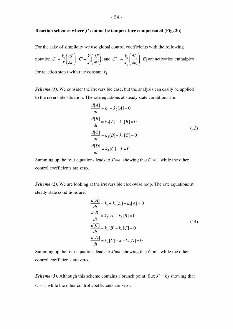
Reaction schemes where J’ cannot be temperature compensated (Fig. 2b)

For the sake of simplicity we use global control coefficients with the following

notation

€

Ci =kiJ'

∂J'∂ki

,

€

C'= k 'J '

∂J'∂k'

, and

€

CiJ j =

kiJ j

∂J j

∂ki

. Ei are activation enthalpies

for reaction step i with rate constant ki.

Scheme (1). We consider the irreversible case, but the analysis can easily be applied

to the reversible situation. The rate equations at steady state conditions are:

€

d[A]dt

= k1 − k2[A] = 0

d[B]dt

= k2[A]− k3[B] = 0

d[C]dt

= k3[B]− k4[C] = 0

d[D]dt

= k4[C]− J '= 0

(13)

Summing up the four equations leads to J’=k1 showing that C1=1, while the othercontrol coefficients are zero.

Scheme (2). We are looking at the irreversible clockwise loop. The rate equations at

steady state conditions are:

€

d[A]dt

= k1 + k5[D]− k2[A] = 0

d[B]dt

= k2[A]− k3[B] = 0

d[C]dt

= k3[B]− k4[C] = 0

d[D]dt

= k4[C]− J '−k5[D] = 0

(14)

Summing up the four equations leads to J’=k1 showing that C1=1, while the other

control coefficients are zero.

Scheme (3). Although this scheme contains a branch point, flux J’ = k1 showing that

C1=1, while the other control coefficients are zero.

- 25 -

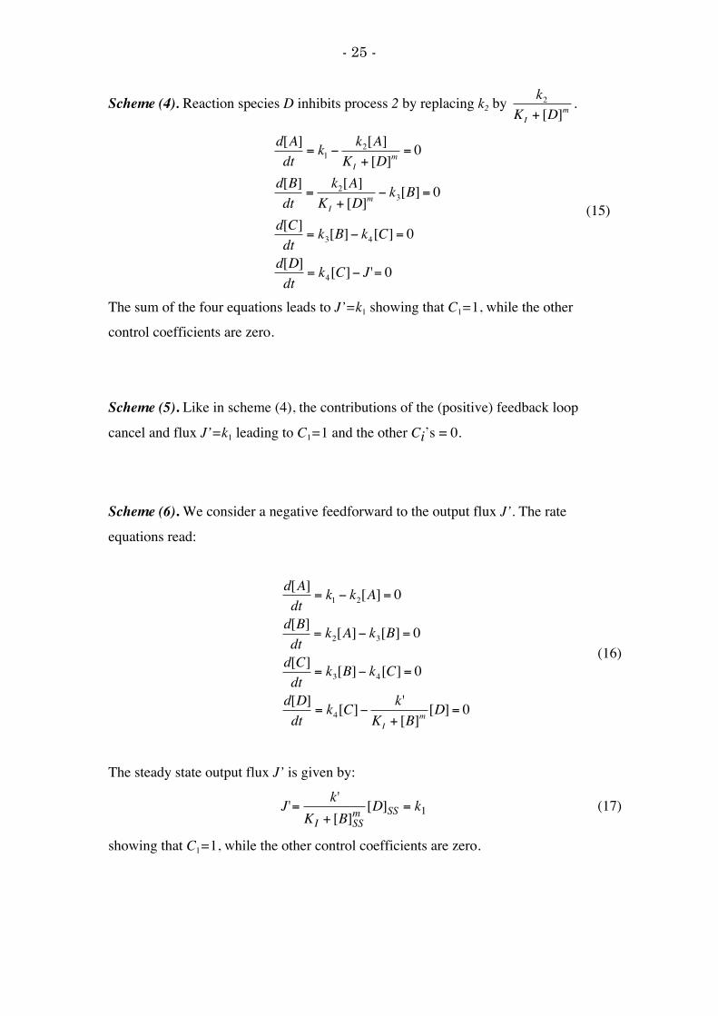
Scheme (4). Reaction species D inhibits process 2 by replacing k2 by

€

k2KI + [D]m

.

€

d[A]dt

= k1 −k2[A]

KI + [D]m= 0

d[B]dt

=k2[A]

KI + [D]m− k3[B] = 0

d[C]dt

= k3[B]− k4[C] = 0

d[D]dt

= k4[C]− J '= 0

(15)

The sum of the four equations leads to J’=k1 showing that C1=1, while the othercontrol coefficients are zero.

Scheme (5). Like in scheme (4), the contributions of the (positive) feedback loop

cancel and flux J’=k1 leading to C1=1 and the other Ci’s = 0.

Scheme (6). We consider a negative feedforward to the output flux J’. The rate

equations read:

€

d[A]dt

= k1 − k2[A] = 0

d[B]dt

= k2[A]− k3[B] = 0

d[C]dt

= k3[B]− k4[C] = 0

d[D]dt

= k4[C]−k '

KI + [B]m[D] = 0

(16)

The steady state output flux J’ is given by:

€

J'= k'KI + [B]SS

m [D]SS = k1 (17)

showing that C1=1, while the other control coefficients are zero.

- 26 -

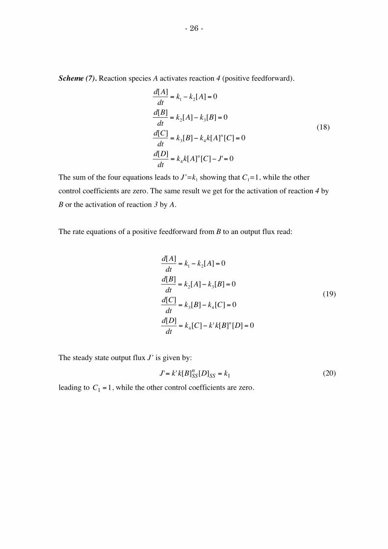
Scheme (7). Reaction species A activates reaction 4 (positive feedforward).

€

d[A]dt

= k1 − k2[A] = 0

d[B]dt

= k2[A]− k3[B] = 0

d[C]dt

= k3[B]− k4k[A]n[C] = 0

d[D]dt

= k4k[A]n[C]− J'= 0

(18)

The sum of the four equations leads to J’=k1 showing that C1=1, while the other

control coefficients are zero. The same result we get for the activation of reaction 4 by

B or the activation of reaction 3 by A.

The rate equations of a positive feedforward from B to an output flux read:

€

d[A]dt

= k1 − k2[A] = 0

d[B]dt

= k2[A]− k3[B] = 0

d[C]dt

= k3[B]− k4[C] = 0

d[D]dt

= k4[C]− k 'k[B]n[D] = 0

(19)

The steady state output flux J’ is given by:

€

J'= k 'k[B]SSn [D]SS = k1 (20)

leading to

€

C1 =1, while the other control coefficients are zero.

- 27 -

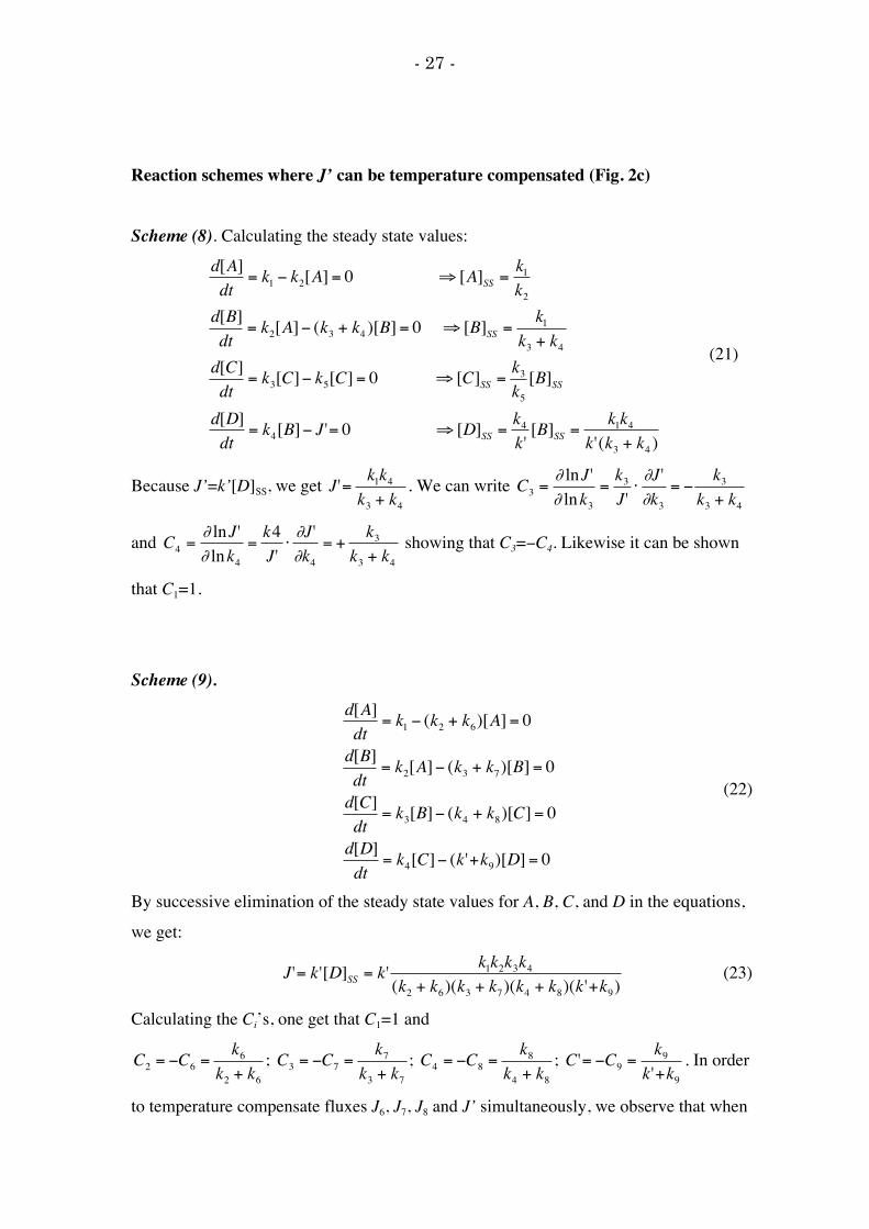
Reaction schemes where J’ can be temperature compensated (Fig. 2c)

Scheme (8). Calculating the steady state values:

€

d[A]dt

= k1 − k2[A] = 0 ⇒ [A]SS =k1k2

d[B]dt

= k2[A]− (k3 + k4 )[B] = 0 ⇒ [B]SS =k1

k3 + k4d[C]dt

= k3[C]− k5[C] = 0 ⇒ [C]SS =k3k5[B]SS

d[D]dt

= k4[B]− J '= 0 ⇒ [D]SS =k4k'[B]SS =

k1k4k'(k3 + k4 )

(21)

Because J’=k’[D]SS, we get

€

J'= k1k4k3 + k4

. We can write

€

C3 =∂ lnJ '∂ lnk3

=k3J'⋅∂J'∂k3

= −k3

k3 + k4

and

€

C4 =∂ lnJ '∂ lnk4

=k4J'⋅∂J'∂k4

= +k3

k3 + k4 showing that C3=−C4. Likewise it can be shown

that C1=1.

Scheme (9).

€

d[A]dt

= k1 − (k2 + k6)[A] = 0

d[B]dt

= k2[A]− (k3 + k7)[B] = 0

d[C]dt

= k3[B]− (k4 + k8)[C] = 0

d[D]dt

= k4[C]− (k'+k9)[D] = 0

(22)

By successive elimination of the steady state values for A, B, C, and D in the equations,

we get:

€

J'= k '[D]SS = k' k1k2k3k4(k2 + k6)(k3 + k7)(k4 + k8)(k '+k9)

(23)

Calculating the Ci’s, one get that C1=1 and

€

C2 = −C6 =k6

k2 + k6;

€

C3 = −C7 =k7

k3 + k7;

€

C4 = −C8 =k8

k4 + k8;

€

C'= −C9 =k9

k'+k9. In order

to temperature compensate fluxes J6, J7, J8 and J’ simultaneously, we observe that when

- 28 -

compensating first J6, this flux depends only on k1, k2 and k6 with

€

C1J6 =1 and

€

C2J6 = −C6

J6 = −k2

k2 + k6 while all the other control coefficients are zero. This leads to the

balance equation

€

E1 + C2J6 (E2 − E6) = 0 (24)

which determines the values of E1, E2 and E6. The condition to temperature compensateJ7 is:

€

E1 + C2J7 (E2 − E6) + C3

J7 (E3 − E7) = 0 (25)

Because

€

C2J6 is generally different from

€

C2J7 , the sum

€

E1 + C2J7 (E2 − E6) in Eq. 20 need

not to be zero, but E3 and E7 can be chosen such that Eq. 20 is satisfied. In this way J6,

J7 and J8 and J’ can be simultaneously temperature compensated when solving thebalance equations 19-22.

€

E1 + C2J8 (E2 − E6) + C3

J8 (E3 − E7) + C4J8 (E4 − E8) = 0 (26)

€

E1 + C2J ' (E2 − E6) + C3

J ' (E3 − E7) + C4J ' (E4 − E8) + CJ ' (E '−E9) = 0 (27)

Scheme 10. The rate equations of this cyclic scheme with steady state conditions read:

€

d[A]dt

= k1 − k2[A]+ k5[D] = 0

d[B]dt

= k2[A]− (k3 + k6)[B] = 0

d[C]dt

= k3[B]− (k4 + k7)[C] = 0

d[D]dt

= k4[C]− (k'+k5)[D] = 0

(28)

By successively eliminating the steady state values [A]SS, [B]SS and [C]SS, an expression

for [D]SS and J’ can be obtained:

€

J'= k ' k1k3k4N

(29)

where N=k’k6k7 + k’k4k6 + k’k3k7 + k’k3k4 + k5k6k7 + k4k5k6 + k3k5k7. Calculating the

control coefficients as

€

Ci =kiJ'

∂J'∂ki

, we get:

- 29 -

C1 = 1, C2 = 0,

€

C3 =k6(k 'k7 + k'k4 + k5k7 + k5k4 )

N,

€

C4 =k7(k 'k6 + k'k3 + k5k6 + k5k3)

N,

€

C5 = −k5(k6k7 + k6k4 + k3k7)

N, C6 = −C3, C7 = −C4, C’ = −C5 with

€

Ci + C'=1i=1

7

∑ .

Scheme (11). Inhibition of J1 by any intermediate. We take as an example the inhibitionof J1 by C with Hill coefficient m = 1. The rate equations with steady state conditions

are:

€

d[A]dt

=k1

KI + [C]1− k2[A] = 0

d[B]dt

= k2[A]− k3[B] = 0

d[C]dt

= k3[B]− k4[C] = 0

d[D]dt

= k4[C]− k '[D] = 0

(30)

leading to

€

J'= k '[D]SS =k1

KI + [C]SS. Eliminating the variables A and B and determining

the positive solution of the steady state value of C:

€

[C]SS =−k4KI + (k4KI )

2 + 4k1k42k4

(31)

J’ can be expressed as:

€

J'= 2k1k4k4KI + k4M

; M = (k4KI2 + 4k1) (32)

Calculating the control coefficients as

€

Ci =kiJ'

∂J'∂ki

, we get:

€

C1 =k4 (KI k4M + k4KI

2 + 2k1)(k4KI + k4M ) ⋅ k4M

,

€

C4 =2k1k4

(k4KI + k4M ) ⋅ k4M,

€

CKI= −

k4KI

(k4KI + k4M );

C2 = C3 = C’ = 0. Note, temperature compensation is only possible because the inhibitor

constant KI (which can be interpreted as a dissociation constant in rapid equilibriumbetween the enzyme that catalyzes step 1 and the inhibitor C) is assumed to be

temperature dependent. The temperature dependence of KI can be described analogously

to the Arrhenius equation by substituting the activation enthalpy with the enthalpy of

formation

€

ΔHI0. In this case the pre-exponential factor AI can still be treated as

temperature independent with AI = exp(−

€

ΔSI0/R) [1]. To describe the temperature

- 30 -

dependence of KI, KM, and Ki in an uniform manner, the enthalpy of formation, for

example for

€

ΔHi0 has been substituted by

€

EaK I in the main text (see also description of

€

EaK I in the Abbreviations and Symbols section). It should also be noted that when

treating KI as a temperature dependent parameter, then the sum of the control coefficients

is generally not one. In this case we get:

€

Cii=1

4

∑ + CKI+ C'= 4k1k4

(k4KI + k4M ) k4M (33)

Scheme (12). Activation of J1 by any intermediate. In order to avoid an exponential

increase of concentrations, n needs to be lower than 1. As an example, we look at theactivation of reaction 1 by intermediate C. The rate equations with steady state conditions

are:

€

d[A]dt

= k1k[C]n − k2[A] = 0, 0 < n <1

d[B]dt

= k2[A]− k3[B] = 0

d[C]dt

= k3[B]− k4[C] = 0

d[D]dt

= k4[C]− k '[D] = 0

(34)

Summing up all steady state equations leads to

€

J'= k '[D]SS = k1k[C]SSn (35)

When adding only the first three equations, we get

€

k1k[C]SSn − k4[C]SS = 0 . Solving for

[C]SS from the last equation and multiplying [C]SS with k4, we get:

€

J'= k3k1kk3

−1n−1

(36)

Calculating the control coefficients as

€

Ci =kiJ'

∂J'∂ki

, we get:

€

C1 = Ck = −1n −1

,

€

C3 =nn −1

, while all other Ci are zero. The sum

€

Ci + C'+Cki=1

4

∑ =n − 2n −1

shows that in

case of a feedback activation of an input flux using n < 1 the summation theorem is notobeyed.

- 31 -

A Simple Representation of the Calvin Benson CycleFig. 5c shows a simple representation of the Calvin Benson cycle with its 3 stages: (i)the reduction phase (flux J2) due to influx of ATP and NADPH produced by the light

reaction together with the output flux of Pi, (ii) the regeneration phase (flux J3) with theoutput flux J6 forming carbohydrates, and (iii) the ATP/NADPH-driven carboxylation

phase (flux

€

J4CO2 ) assimilating CO2 [37]. The rate constant

€

k4CO2 is assumed to be

dependent on the partial but constant CO2 pressure.

The rate equations and steady state conditions are given by the following equations:

€

d[A]dt

= k3[C]− (k4CO2 + k6)[A] = 0

d[B]dt

= k4CO2 [A]+ k1 − k2[B] = 0

d[C]dt

= k2[B]− (k3 + k5)[C] = 0

(37)

Eliminating variables C and B and calculating

€

J4CO2=

€

k4CO2 [A]SS leads to

€

J4CO2=

€

k4CO2k1k3L

, L = k5k4CO2 + k5k6 + k3k6 (38)

The control coefficients

€

Ci =kiJ4CO2

∂J4CO2

∂ki

are C1 = 1, C2 = 0,

€

C3 = −C5 =k5(k4 + k6)

L,

and

€

C4 = −C6 =k6(k5 + k3)

L. The assimilation of CO2 can be temperature compensated

because of the ”balance” between the input and output fluxes.

- 32 -

Figure legends

Fig. 1. Simple model of transcription (mRNA synthesis with rate constant k1) and

translation (protein synthesis with rate constant k3) of an enzyme E which catalyzes

the conversion of S → P. All reactions are considered to be first-order, except reaction

rate

€

J5 =d[P]dt

=k5catess[S]KM + [S]

. The other constants are: k2, rate constant for mRNA

degradation; k4, rate constant of enzyme degradation. KM and

€

k5cat are the Michaelis

constant and the turnover number, respectively.

Fig. 2. Network models. (a) General scheme depicting input, internal and output

fluxes. (b) Reaction schemes where the steady state flux J’ cannot be temperaturecompensated. (c) Reaction schemes where J’ can be temperature compensated (see

Supplementary Material). For the sake of simplicity global control coefficients

(without an asterisk) are used and defined as

€

Ci =kiJ'

∂J'∂ki

,

€

C'= k 'J '

∂J'∂k'

, and

€

CiJ j =

kiJ j

∂J j

∂ki

, where ki is the rate constant of reaction step i. Positive/negative signs

indicate positive/negative feedforward or feedback loops leading to activation or

inhibtion of a particular process. For a description about the kinetics using activationconstant k and inhibition constant KI in positive or negative feedforward/feedback

loops, see main text. Control coefficients with respect to k and KI are defined as

€

Ck =kJ'

∂J'∂k

and

€

CKI=KI

J'∂J'∂KI

.

Fig. 3. Kinetics of compensated and uncompensated network (8) (Fig. 2c). At 25°C

the rate constants have the following (arbitrary chosen) values k1=1.7 (time units)−1,

k2=0.1 (time units)−1, k3=0.5 (time units)−1, k4=1.5 (time units)−1, k5=1.35 (time units)−1,

k6=0.7 (time units)−1. Initial concentrations of A, B, C, and D (at t=0) are zero. The

- 33 -

control coefficients (as defined in the legend of Fig. 2) at 25°C are

€

C1J '=1.0,

€

C3J '=−0.250,

€

C4J '=0.250. (a) Open squares show the exponential increase of J’ as a

function of temperature for the uncompensated network (all activation enthalpies

being taken 67 kJ/mol; note:

€

Eak2 ,

€

Eak5 and

€

Eak6 do not matter, because the associated

control coefficients are zero). Open diamonds show the effect of static temperature

compensation of J’ when using

€

Eak1 =26 kJ/mol,

€

Eak3 =120 kJ/mol and

€

Eak4 =22 kJ/mol.

Solid circles show the effect of dynamic temperature compensation by keeping

€

Eak3

and

€

Eak4 constant but increasing

€

Eak1 (described as

€

E1dynamic) with increasing

temperatures as shown in the inset. For each temperature T

€

E1dynamic was estimated

according to the equation

€

E1dynamic (T) = Ea

k1 − 0.5 CiJ ' (T)

i∑ Ea

ki , where the Ci(T)’s were

calculated at temperature T. (b) Transient kinetics of the uncompensated network (Fig.

3a) when applying a 15°C→35°C temperature step at t=300 time units. The inset

shows the details of the response kinetics. The difference in the J’ steady state levels

at 15°C and 35°C is clearly seen. (c) Transient kinetics of the static temperature

compensated network (Fig. 3a) when applying a 15°C→35°C temperature step at

t=300. The inset shows transient kinetics when a 35°C→15°C temperature step is

applied. (d) Fluxes J1 and J3 as a function of temperature in the static temperature

compensation of J’ (Fig. 3a).

Fig. 4. Experimental evidence for dynamic temperature compensation. (a)

Temperature dependent metabolic activity of S. cerevisiae. The cells were acclimated

at anaerobic conditions to 15°C, 22.5°C and 30°C. The anaerobic metabolic activity

of the cells was measured as the overall generated differential power DP in mJ min-1

per mg of wet cell biomass using Differential Scanning Microcalorimetry

- 34 -

(0.5°C/min). The curves are the average of n=4 at 15°C, n=16 at 22.5°C, and n=5 at

30°C. The large dots indicate metabolic activities at the corresponding acclimation

temperatures with standard deviations. For temperatures higher than 40°C the

produced heat was lowered by cell death. (b) Arrhenius plots for the three acclimation

temperatures. Activation enthalpies were estimated by linear regression between 4°C

(0.0036 K-1) and 40°C (0.0032 K-1) for acclimation at 15°C and 22.5°C, and by

linear regression between 10°C (0.0035 K-1) and 40°C (0.0032 K-1) for acclimation

at 30°C. Estimated activation enthalpies are: 44.8 kJ/mol (acclimation at 15°C), 52.6

kJ/mol (acclimation at 22.5°C), and 75.6 kJ/mol (acclimation at 30°C).

Fig. 5. Mimicking temperature compensation and temperature adaptation of

photosynthesis in higher plants. (a) Photosynthetic flux of plant species living in hot

(S. albicans), temperate (S. anglica) and cold environments (T. oblongifolia).

Redrawn from Ref. [7]. (b) Temperature response of a single branch point (flux J4 of

scheme (8)) with different activation enthalpy combinations. For the sake of

simplicity Ei are activation enthalpies for reaction step i with rate constant ki. For

details see Supplementary Material. (1) E1=190 kJ/mol, E3=290 kJ/mol, E4=20 kJ/mol;

(2) E1=70 kJ/mol, E3=190 kJ/mol, E4=20 kJ/mol; (3) E1=20 kJ/mol, E3=93 kJ/mol,

E4=23 kJ/mol. In addition, the value of k1 at 25°C has been reduced from 1.7 (time

units)−1 to 0.5 (time units)−1. All other rate constants and Tref were as described in Fig.

3. (c) A minimal model of the Calvin Benson Cycle with reduction phase (fluxes J1,

J2, J5), regeneration phase (fluxes J3, J6) and carbon dioxide assimilation (flux

€

J4CO2 ).

(d)

€

J4CO2 as a function of temperature for 3 parameter set combinations (curves 1-3).

Joint rate constant values for all 3 curves (defined at Tref=25°C): k2=0.1 (time units)−1,

- 35 -

k3=0.5 (time units)−1,

€

k4CO2=1.5 (time units)−1

(concentration units)−1 , k5=1.35 (time

units)−1 , k6=0.7 (time units)−1. Ci values (at Tref=25°C): C1 = 1, C2 = 0, C3 = −C5 =

0.895, C4 = −C6 = 0.390. k1 values and activation enthalpy combinations: (1) k1=2.2

(concentration units) (time units)−1 E1 = 92 kJ/mol, E3 = 90 kJ/mol, E4 = 40 kJ/mol, E5

= 50 kJ/mol, E6 = 220 kJ/mol; (2) k1=1.4 (concentration units) (time units)−1 E1 = 62

kJ/mol, E3 = 70 kJ/mol, E4 = 40 kJ/mol, E5 = 50 kJ/mol, E6 = 220 kJ/mol; (3) k1=0.5

(concentration units) (time units)−1 E1 = 30.5 kJ/mol, E3 = 39 kJ/mol, E4 = 40 kJ/mol,

E5 = 60 kJ/mol, E6 = 70 kJ/mol with

€

Cii=1

6

∑ Ei = 0.012 kJ/mol. Note, because C2=0, k2

and activation enthalpy E2 do not influence the steady state value of

€

J4CO2 and its

temperature profile. Also note, because C1 = 1,

€

J4CO2 values can be changed by

changing k1, but without changing the form of the temperature profile for

€

J4CO2 .

mRNA

geneE

S P

k1

k2k3

k4

k5 , KM

Ruoff et al. : Temperature Compensation...... Figure 1

cat

A B C Dk1 kʼ (1)

No temperature compensation of Jʼ possible

IkIl

IjIi

inputfluxes

outputfluxes

a

b

cTemperature compensation of Jʼ possible

(8)A B

C

D

k1 k2 k3

k4 kʼ

k5

C1 = 1; C3 = − C4; C3 < 0; C4 > 0; all other Ciʼs

= 0

J1 J2

J5 J3

J4 Jʼ

internalfluxes

C1

= 1,

all

othe

r Ciʼs

= 0

A B C Dk1 kʼ

(9)

k2 k3 k4

k6 k7 k8 k9

C2 = −C6; C3 = −C7; C4 = −C8; Cʼ = −C9

C2, C3, C4, Cʼ > 0; C6, C7, C8, C9 < 0C1 = 1;

J1 J6 J2 J7

J3 J4 J8 J9

Jʼ

Jʼ

B

k2

k3

A

C

D

k1

k4

kʼ

k5

k6

k7

(10)

C1 = 1; C2 = 0;

C5 = −Cʼ; Cʼ > 0;

C6 = −C3; C3 > 0;

C7 = −C4; C4 > 0;

Jʼ(2)

A

B

C

D

k1

kʼ

J1

k2

k3 k4

k5

Jʼ

(3) AB

CDk1 kʼ Jʼ

C1 > 0, C4 > 0, CKI

A B C Dk1 k2 k3 k4 kʼ (11)KI , m

< 0. All other Ciʼs are zero.

Jʼ

A B C Dk1 k2 k3 k4 kʼ (12)

k, n < 1

C1 < 0, Ck < 0, C3 > 0. Jʼ

(4) A B C Dk1 k2 k3 k4 kʼ

KI , m

Jʼ

(5) A B C Dk1 k2 k3 k4 kʼ

k, n

Jʼ

Ruoff et al. : Temperature Compensation...... Figure 2

A B C Dk1 k2 k3 k4 kʼ (6)

KI , m

Jʼ

(7) A B C Dk1 k2 k3 k4 kʼ

k, n

Jʼ

k2 k3 k4

k-2 k-3 k-4

0

2

4

6

8

0 100 200 300 400 500 600

flux

J', a

.u.

35°C

c

15°C

time, a.u.

(static)compensation

0

0.5

1

1.5

2

2.5

3

3.5

15 20 25 30 35temperature, °C

a

flux

J', a

.u.

uncompensated

'static'compensation

'dynamic'compensation

15

20

25

30

35

40

15 20 25 30 35

E 1dyna

mic, k

J/mol

temperature, °C

0

0.5

1

1.5

2

2.5

3

3.5

4

0 100 200 300 400 500 600flu

x J',

a.u

.time, a.u.

b

uncompensated

35°C15°C

00.51

1.52

2.53

3.5

290 300 310 320

flux

J', a

.u.

time, a.u.

15°C 35°C

00.20.40.60.81

1.2

200 250 300 350 400

flux

J', a

.u.

time, a.u.

35°C 15°C

0

0.5

1

1.5

2

2.5

15 20 25 30 35

flu

x, a

.u.

temperature, °C

J1 = J2 = J3 + J

4

J' = J1 − J

3 = J4

J3 = J

5

d

Ruoff et al. : Temperature Compensation...... Figure 3

0

0.5

1

1.5

2

2.5

3

3.5

0 10 20 30 40 50 60

DP,

mJ m

in-1

mg-1

temperature, °C

15°C

30°C

dT/dt = 0.5°C min-1

a 22.5°C

15°C22.5°C

-1.5

-1

-0.5

0

0.5

1

1.5

3 3.2 3.4 3.6

ln D

P

1000/T, K-1

b15°C

22.5°C30°C

Ruoff et al. : Temperature Compensation...... Figure 4

c

0102030405060

010

2030

4050

60

S. a

lbic

ans

S. a

nglic

aT.

obl

ongi

folia

photosynthetic rate, µmol m-2

s-1

leaf

tem

pera

ture

, °C

a

0

0.51

1.52

2.5 10

1520

2530

3540

tem

pera

ture

, °C

1 2 3b

flux J', a.u.

singl

e br

anch

poi

ntFi

g. 2

c, sc

hem

e (8

)

0

0.1

0.2

0.3

0.4

0.5

0.6 10

1520

2530

3540

J4

CO , a.u. 2

tem

pera

ture

, °C

1 2dcy

clic

sche

me

Fig.

5c

3

Ruof

f et a

l: Te

mpe

ratu

re C

ompe

nsat

ion.

....

F

igur

e 5