Embed Size (px)
Citation preview
water
Article
Temperature and Consolidation Sensing NearDrinking Water Wells Using Fiber BraggGrating Sensors
Sandra Drusová 1,2,* , R. Martijn Wagterveld 1 , Karel J. Keesman 1,3 andHerman L. Offerhaus 2
1 Wetsus, European Centre of Excellence for Sustainable Water Technology, Oostergoweg 9,8911 MA Leeuwarden, The Netherlands; [email protected] (R.M.W.);[email protected] (K.J.K.)
2 Optical Sciences, University of Twente, Hallenweg 23, 7522 NH Enschede, The Netherlands;[email protected]
3 Mathematical and Statistical Methods—Biometris, Wageningen University, P.O. Box 16,6700 AA Wageningen, The Netherlands
* Correspondence: [email protected]
Received: 13 November 2020; Accepted: 15 December 2020; Published: 19 December 2020 �����������������
Abstract: Drinking water wells require continuous monitoring to prevent groundwater-relatedissues such as pollution, clogging and overdrafting. In this research, optical fibers with fiberBragg grating sensors were placed in an aquifer to explore their potential use in long-term wellmonitoring. Fiber Bragg grating sensors were simultaneously sensitive to consolidation strain andtemperature, and these two responses were separated by creating autoregressive consolidationmodels. Consolidation responses from these multiple sensors were rescaled to obtain pressuredistribution along the depth. Pressure and temperature data showed impermeable soil layers andlocations where groundwater accumulated. Time development of temperature along the fiberrevealed oxidation of minerals and soil layers with varying permeability. Fiber Bragg gratingsensors are useful tools to examine subsurface processes near wells and they can show the first signsof clogging.
Keywords: fiber Bragg grating; ARX model; temperature; consolidation; well monitoring; subsurfaceiron removal; clogging
1. Introduction
Groundwater, as the cleanest source for public drinking water supply, is extracted from aquifersthrough wells. Series of pumping tests are performed before a well starts long-term extraction.Pumping tests are the most suitable way to determine groundwater quality, aquifer properties andappropriate depth of the pump from single observation points [1]. During a pumping test, groundwateris extracted from the well at a controlled rate and water levels are observed in monitoring wells.The aquifer properties calculated from pumping tests are hydraulic conductivity, storage coefficient,and specific yield [2]. These values are used to estimate the radius of influence of the area affected bypumping [3].
All aforementioned parameters might change during a long-term operation, so drinking waterextraction wells need to be continuously monitored. A decrease in the well yield and water quality isthe first sign of well clogging [4]. Continuously decreasing water levels in monitoring wells indicategroundwater overdrafting [5]. Consequently, groundwater gets extracted from a larger radius thaninitially expected and water quality might degrade due to intrusion of polluted or saline water.
Water 2020, 12, 3572; doi:10.3390/w12123572 www.mdpi.com/journal/water
Water 2020, 12, 3572 2 of 17
When overdrafting continues, it might result in permanent land subsidence [6]. The process causingland subsidence is extraction-related consolidation. Consolidation is defined as volumetric changesin soil due to pressure changes. Groundwater extraction lowers the pressure in soil which results invertical compression (strain) in the aquifer [7]. When the extraction stops and water levels repeatedlydo not recover, compression of the aquifer accumulates [8]. Long-term monitoring of the wells isimportant to prevent all groundwater-related issues.
Commonly monitored parameters in extraction well fields are flowrate of the wells,pressure (water levels), temperature, water conductivity, and water quality (chemical composition) [9].Another important parameter which needs to be monitored is groundwater flow around the well,both its magnitude and direction. Groundwater flow can be measured directly in the monitoringwells using borehole flowmeters [10] and the spatial flow field near wells can be predicted usinggroundwater flow models. The limitation of regional groundwater flow models is a lack of field datafor the model input [11]. One way the models can be improved is by using input data with a higherspatial resolution collected by fiber-optic sensors [12].
Promising fiber-optic sensors for groundwater monitoring are fiber Bragg grating (FBG) sensorsbecause they can measure multiple parameters simultaneously and spatial resolution can becustomized [13]. FBG sensors are used to measure, for example, temperature and pressure [14,15],and pH [16]. An FBG sensor consists of a refractive index modulation in the fiber core with a periodΛ. The grating acts as a mirror only for the Bragg wavelength λ0—a wavelength that matches thegrating period:
λ0 = 2ne f f Λ, (1)
where ne f f is the effective refractive index for the propagating light mode in the fiber. FBG sensors aresimultaneously sensitive to temperature and mechanical strain. FBG sensors can measure multipleparameters if these are translated to strain through FBG packaging. Sensitivity to a certain parametercan also be customized by choice of packaging. FBG sensors have a wide range of applications inmonitoring subsurface structures. They are employed to prevent landslides [17], monitor the stabilityof dams [18,19], or measure pressure and temperature in oil wells [20]. Groundwater-related FBGresearch is focused on measuring pressure and temperature at remediation sites [21] and subsidencecaused by groundwater extraction [22,23].
In this paper, we explore the potential of FBG sensors for groundwater monitoring in adrinking water well field. The wells in the field are used for groundwater extraction and injection.A small volume of the extracted water is injected into the ground for subsurface iron removal [24],causing clogging in soil instead of the well screen. The injected water can be used as a thermaltracer for groundwater flow and allows us to identify clogged soil layers. FBG sensors weredeployed for measuring temperature and consolidation strain and a new method of separatingthese effects is presented. FBG consolidation response was rescaled to show pressure distributionclose to a well. The results from the FBG sensors are compared to reference sensors for temperature,pressure and flowrate.
2. Materials and Methods
2.1. Experimental Site and Sensor Installation
The location of this study was a drinking water extraction field in Hengelo, Gelderland,The Netherlands. There are 12 wells in the area extracting with a flowrate of 128 m3/h, see Figure 1afor their location. Groundwater from this area is rich in iron. Dissolved iron ions cause an unwantedyellow colorization in the drinking water, so they need to be removed before the water is sent into thedistribution network. To remove iron, a part of the extracted water is enriched with dissolved oxygenand is periodically injected back into the ground with half of the normal extraction rate. As a result,iron oxides and hydroxides precipitate in soil.
Water 2020, 12, 3572 3 of 17
0 50 100meters
100
200
300
400
w1
Cluster 1
Cluster 2
Wells
Cluster 3
4
8
w1
C
BA
P2,P3
P4
P1
P5,P6
20 4meters
FBG fibers
Piezometers
Well 1
(a) (b)
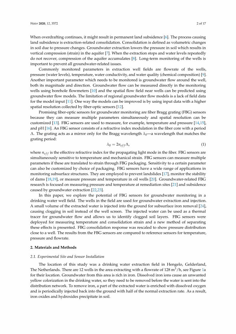
Figure 1. A map of the drinking water well field: (a) location of the extraction wells sorted in clusters.The area in the white rectangle is displayed in (b). (b) Location of the fiber Bragg grating (FBG) bundlesand reference piezometers near well 1. Data from sensors circled in red is compared in the Section 3.
Data from multiple sensors are processed and compared in this paper:
• FBG sensors: consolidation and temperature• reference divers: pressure and temperature• weather station: atmospheric pressure• flowmeter: horizontal flowrate in well w1• status of 12 wells: on/off
FBG sensors and reference divers were installed at a distance of less than 10 m from well w1(Figure 1b). Boreholes were drilled down to 38 m depth using the flush drilling technique. FBG fiberbundles with sensors were glued to a fishing line with a weight to keep the fibers straight when theywere placed in open boreholes. The boreholes were refilled with the original sediment, although thenatural sediment layering was not precisely reconstructed. Divers are pressure and temperature sensorsthat were suspended in piezometer tubes. Six divers (TD reference diver, van Essen Instruments, Delft,The Netherlands) were installed at the depth of 10 m.
In total, three FBG fiber bundles A, B, C were installed near the well, each bundle with24 sensors equally spaced by 0.7 m, starting from 17 m depth to cover the length of the well screen(17.8–32 m). Each FBG bundle contains three fibers protected by a 1-mm thick Teflon tube with3 mm diameter (Loptek, Berlin, Germany). The FBG bundle was a part of a sensing cable with DTS(distributed temperature sensing) fibers, a looped heating wire and a nylon fishing line. All parts weretied using tie wraps and glued with silicon.
FBG data was collected using an FBG interrogator (Hyperion si155, LUNA, Roanoke, VA, USA)controlled by a microcontroller (Raspberry Pi model 3B, Raspberry Pi Foundation, Cambridge, UK).The microcontroller was programmed to autonomously collect the data and report the state of theunit. FBG data had a sampling period of 2.1 s. Diver data had a sampling period of 5 s. Since diverswere placed inside piezometers, corrections had to be made to get data comparable to the FBG sensorsplaced in direct contact with the soil. Divers measure absolute pressure pdiver, which is a combinationof hydrostatic pressure p and atmospheric pressure patm. Hydrostatic (pore pressure) was obtained as:
p = pdiver − patm (2)
Water 2020, 12, 3572 4 of 17
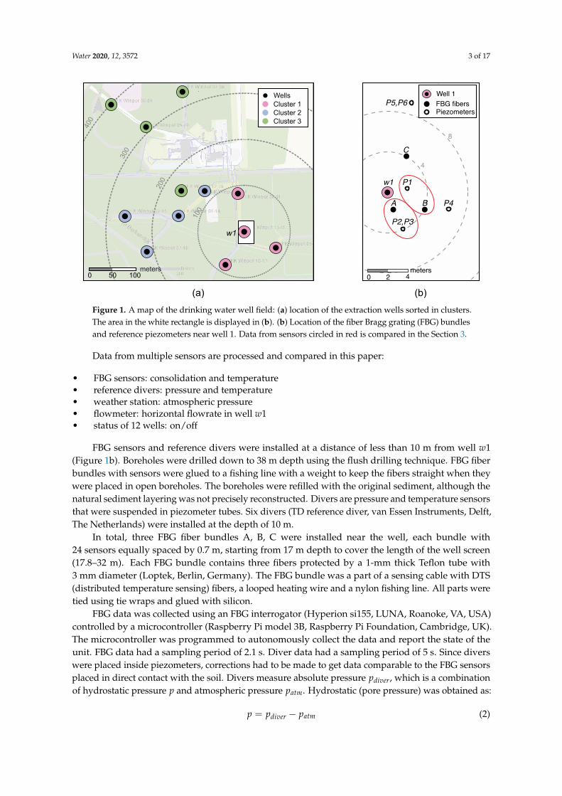
Atmospheric pressure was measured using a pressure sensor in a weather station installed at thesite. It is important to realize that for most of the time, divers measured water temperature inside ofthe piezometer tube, not the groundwater temperature directly. The divers were suspended at thedepth of 10 m, while piezometers screens were at 17.8–19.8 m and 22.5–24.5 m. When the nearest wellstarts extracting, groundwater flows through the piezometer screen but it does not reach the divers(see Figure 2a). When the water level in the piezometer drops, the diver measures the temperature ofthe water column above. This temperature tends to be higher due to stratification. When the nearestwell stops extracting (see Figure 2b), the water level in the piezometer rises and the groundwaterflows towards the diver. Inflowing water gets mixed with the water inside the piezometer and thetemperature is equalized. Divers, therefore, measure the temperature of the groundwater in the aquiferonly for a short time after the nearest well stops extracting.
ΔTΔT
ΔTdiver
ΔTΔT
(a) (b)
Figure 2. A diver installed in a piezometer several meters above the piezometer screen. (a) When thenearby well starts extracting, the extracted groundwater does not reach the diver. (b) When the nearbywell stops extracting, groundwater flows up to the diver and the temperature change at that momentcorresponds more closely to the groundwater temperature.
Horizontal flowrate in w1 was measured using a propeller flowmeter (van Essen Instruments,Delft, The Netherlands). The flowmeter was lowered inside the well during extraction andmeasurement was taken every 0.5 m, in the depths of the well screen. This measurement wastaken shortly after the construction of the well in March 2000. All other presented data was takenin 2018–2019.
In Drusová et al. [25] we examined which effects cause a measurable response of the FBG sensorsin this well field. It was discovered that the FBG sensors measure predominantly soil consolidationcaused by groundwater extraction. FBG sensors are also sensitive to temperature changes. Pressure anddrag force from the flow did not cause any FBG response. FBG response ∆λ in this well field hastwo components:
∆λ = ∆λc + ∆λT (3)
where ∆λc is the consolidation strain contribution and ∆λT is the temperature contribution. We presenta method to isolate each contribution and convert them to temperature and pressure.
2.2. Pressure Sensing
Groundwater temperature is quite stable with seasonal variations being lower than 0.5 °C.Unless water has been injected into the ground, the temperature contribution to the FBG response canbe neglected:
∆λ = ∆λc (4)
Water 2020, 12, 3572 5 of 17
The installed FBG sensors can measure pressure indirectly through consolidation. The FBGconsolidation (strain) response depends on the pressure change ∆p, the initial Bragg wavelength λ0,the compressibility of the soil (represented as Young’s modulus Esoil and Poisson’s ratio νsoil) and afriction coefficient β between the FBG packaging and soil [25]:
∆λc
λ0=
(1 + νsoil)(1 − 2νsoil)
(1 − νsoil)Esoil(1 − pe)β∆p. (5)
Consolidation strain from the soil is coupled to a wavelength shift through the strain-opticcoefficient pe = 0.22. The amplitude of the consolidation itself depends on the distance to a well.
The friction coefficient and soil compressibility are difficult to measure separately. However, if thepressure change ∆p is known, it is possible to calculate one constant scaling factor F for each sensorwhich includes the effect of both soil compressibility and friction:
F =∆λc
λ0∆p=
(1 + νsoil)(1 − 2νsoil)
(1 − νsoil)Esoil(1 − pe)β. (6)
Scaling factors F were calculated from a dataset where the nearest well w1 was not extracting.Pressure changes were caused by the extraction from further wells in the field. In this case,∆ p measured in all piezometers P1 − P6 was nearly equal even though the piezometer screensare located at different depths (12–37 m). Since the FBG bundles are located within 10 m distance ofthe piezometers at 17–33.1 m depth, it can be assumed that the ∆p measured by all FBG sensors isequal to the ∆p measured by the divers.
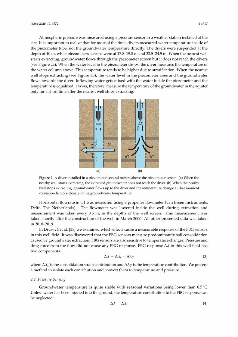
The ∆p from the divers was averaged and this curve was used to calculate the scaling factorsF. The averaged ∆p and FBG curves were parsed into several intervals in such a way that ∆p ismonotonically increasing or decreasing in the interval, see Figure 3. Since FBG sensors also measuretemperature, parsing the FBG response into smaller intervals minimizes the temperature contributionbecause the temperature varies at much larger time scales. The scaling factor F for each FBG sensorwas calculated using Equation (6) in these intervals and averaged. Data from noisy FBG sensors wasdiscarded. The sensors were considered noisy if their overall response to pressure changes caused byw1 was smaller than 2 pm (signal-to-noise ratio 2). The noise level of FBG sensors is dominated by theFBG interrogator, which has a noise level of 1 pm.
0 0.5 1 1.5 2 2.5
Time (days)
−3
−2
−1
0
1
2
3
pfr
om
div
ers
(P
a)
x103
Figure 3. Average pressure change measured by all divers when w1 was not extracting. The pressurecurve is parsed into several intervals divided by dashed lines where the scaling factor F was calculated.
The scaling factor F for each FBG sensor was then used to scale the measured data and calculate∆p when w1 was extracting:
∆p =∆λc
Fλ0(7)
Water 2020, 12, 3572 6 of 17
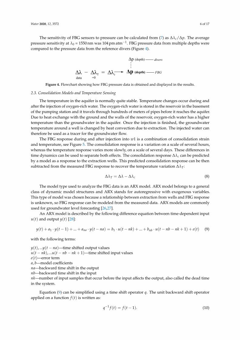
The sensitivity of FBG sensors to pressure can be calculated from (7) as ∆λc/∆p. The averagepressure sensitivity at λ0 = 1550 nm was 104 pm atm−1. FBG pressure data from multiple depths werecompared to the pressure data from the reference divers (Figure 4).
Δλ − =ΔλT cΔλdata =0
Δp (depth) FBG
Δp (depth) divers
Figure 4. Flowchart showing how FBG pressure data is obtained and displayed in the results.
2.3. Consolidation Models and Temperature Sensing
The temperature in the aquifer is normally quite stable. Temperature changes occur during andafter the injection of oxygen-rich water. The oxygen-rich water is stored in the reservoir in the basementof the pumping station and it travels through hundreds of meters of pipes before it reaches the aquifer.Due to heat exchange with the ground and the walls of the reservoir, oxygen-rich water has a highertemperature than the groundwater in the aquifer. Once the injection is finished, the groundwatertemperature around a well is changed by heat convection due to extraction. The injected water cantherefore be used as a tracer for the groundwater flow.
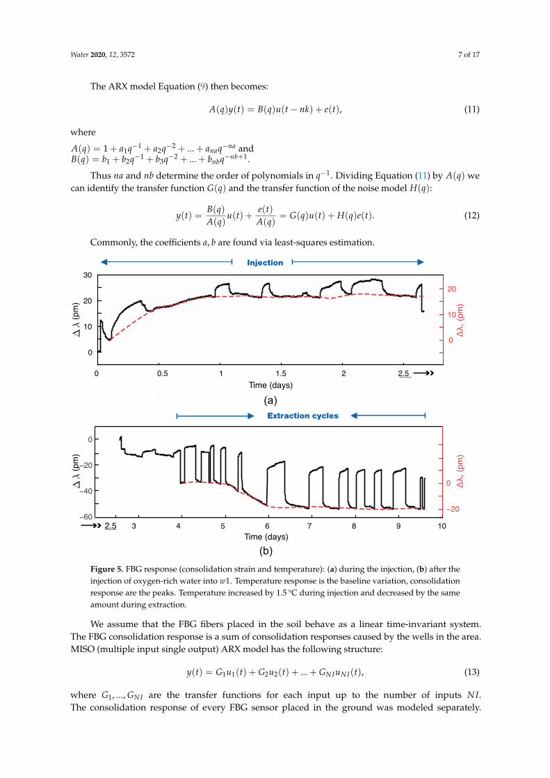
The FBG response during and after injection into w1 is a combination of consolidation strainand temperature, see Figure 5. The consolidation response is a variation on a scale of several hours,whereas the temperature response varies more slowly, on a scale of several days. These differences intime dynamics can be used to separate both effects. The consolidation response ∆λc can be predictedby a model as a response to the extraction wells. This predicted consolidation response can be thensubtracted from the measured FBG response to recover the temperature variation ∆λT :
∆λT = ∆λ − ∆λc (8)
The model type used to analyze the FBG data is an ARX model. ARX model belongs to a generalclass of dynamic model structures and ARX stands for autoregressive with exogenous variables.This type of model was chosen because a relationship between extraction from wells and FBG responseis unknown, so FBG response can be modeled from the measured data. ARX models are commonlyused for groundwater level forecasting [26,27].
An ARX model is described by the following difference equation between time-dependent inputu(t) and output y(t) [28]:
y(t) + a1 · y(t − 1) + ... + ana · y(t − na) = b1 · u(t − nk) + ... + bnb · u(t − nb − nk + 1) + e(t) (9)
with the following terms:
y(t), ...y(t − na)—time shifted output valuesu(t − nk), ...u(t − nb − nk + 1)—time shifted input valuese(t)—error terma, b—model coefficientsna—backward time shift in the outputnb—backward time shift in the inputnk—number of input samples that occur before the input affects the output, also called the dead timein the system.
Equation (9) can be simplified using a time shift operator q. The unit backward shift operatorapplied on a function f (t) is written as:
q−1 f (t) = f (t − 1). (10)
Water 2020, 12, 3572 7 of 17
The ARX model Equation (9) then becomes:
A(q)y(t) = B(q)u(t − nk) + e(t), (11)
where
A(q) = 1 + a1q−1 + a2q−2 + ... + anaq−na andB(q) = b1 + b2q−1 + b3q−2 + ... + bnbq−nb+1.
Thus na and nb determine the order of polynomials in q−1. Dividing Equation (11) by A(q) wecan identify the transfer function G(q) and the transfer function of the noise model H(q):
y(t) =B(q)A(q)
u(t) +e(t)A(q)
= G(q)u(t) + H(q)e(t). (12)
Commonly, the coefficients a, b are found via least-squares estimation.
0
10
20
30
(pm
)
Δλ
T(p
m)
0 0.5 1 1.5 2 2.5
Injection
Time (days)
−60−20
−400
−20
0
Extraction cycles
2.5 3 4 5 6 7 8 9 10
(a)
(b)
Time (days)
(pm
)
0
10
20
Δλ
T(p
m)
Figure 5. FBG response (consolidation strain and temperature): (a) during the injection, (b) after theinjection of oxygen-rich water into w1. Temperature response is the baseline variation, consolidationresponse are the peaks. Temperature increased by 1.5 °C during injection and decreased by the sameamount during extraction.
We assume that the FBG fibers placed in the soil behave as a linear time-invariant system.The FBG consolidation response is a sum of consolidation responses caused by the wells in the area.MISO (multiple input single output) ARX model has the following structure:
y(t) = G1u1(t) + G2u2(t) + ... + GNIuNI(t), (13)
where G1, ..., GNI are the transfer functions for each input up to the number of inputs NI.The consolidation response of every FBG sensor placed in the ground was modeled separately.
Water 2020, 12, 3572 8 of 17
The output data for each model was the wavelength shift ∆λ of an FBG sensor and input datawas the status of the 12 extraction wells. The status is a binary input represented as 0-off, 1-on,measured with a sampling period of 1 min. The FBG data was smoothed with a 2 min moving averageand downsampled to 1 min period to match the pump data.
The optimal number of parameters for the models was chosen by comparing each estimatedparameter value to its standard deviation to prevent overfitting. There were more b coefficientsassigned to the input from the nearest well to model this most dominant contribution more accurately.The time delay between inputs and output also varied. The input from the nearest well had no timedelay and all other inputs were modeled with a delay of 1 sample (1 min). The delay corresponds tothe time it takes to mobilize large volumes of water from a distance larger than 80 m. The number ofparameters used for the model is shown in Table 1.
Table 1. The number of the autoregressive with exogenous variables (ARX) model parameters used forthe FBG consolidation models.
Output Input Well∆λ w1 w2 − 12
na 6nb 8 2nk 0 1
In total, 24 ARX models were created for all FBG sensors at location A and 24 models for location B(see Figure 1b). The performance of the models was evaluated in terms of the root mean square error(RMSE) between modeled and measured data. The model requires training data not influenced bytemperature. Temperature changes during the training and the validation period were measured bythe divers and they were smaller than 0.1 ◦C, which translates into 1 pm of ∆λ. 1 pm corresponds to thenoise level of the interrogator so that the temperature contribution in the training and validation datawas negligible. The length of the training dataset was 5 days and 7 days for the validation. Data forthe training was chosen in such a way that all 12 input trajectories were unique to correctly estimatethe contribution of each input to the FBG response.
Since the temperature changes obtained from ∆λ were expected to be smooth, a moving averagefilter was used on ∆λT to reduce errors caused by imperfect model predictions. Without any furtherstrain effects, the temperature change ∆T can be calculated from ∆λT as [29]:
∆T =∆λTαTλ0
(14)
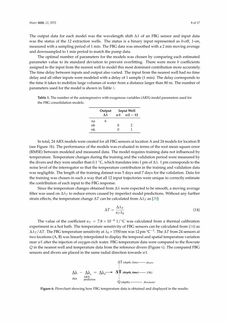
The value of the coefficient αT = 7.8 × 10⁻⁶ 1/◦C was calculated from a thermal calibrationexperiment in a hot bath. The temperature sensitivity of FBG sensors can be calculated from (14) as∆λT/∆T. The FBG temperature sensitivity at λ0 = 1550 nm was 12 pm °C−1. The ∆T from 24 sensors attwo locations (A, B) was linearly interpolated to display the temporal and spatial temperature variationnear w1 after the injection of oxygen-rich water. FBG temperature data were compared to the flowrateQ in the nearest well and temperature data from the reference divers (Figure 6). The compared FBGsensors and divers are placed in the same radial direction towards w1.
Δλ − =Δλ Δλc T
dataARXprediction
ΔT (depth, time)
ΔT (depth, time) divers
FBG
Q (depth) flowmeter
Figure 6. Flowchart showing how FBG temperature data is obtained and displayed in the results.
Water 2020, 12, 3572 9 of 17
3. Results and Discussion
3.1. Pressure (FBG Sensors vs. Divers)
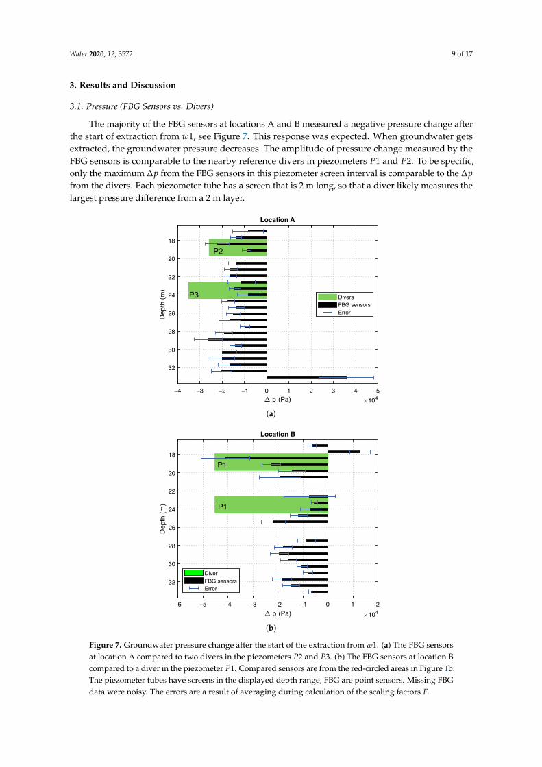
The majority of the FBG sensors at locations A and B measured a negative pressure change afterthe start of extraction from w1, see Figure 7. This response was expected. When groundwater getsextracted, the groundwater pressure decreases. The amplitude of pressure change measured by theFBG sensors is comparable to the nearby reference divers in piezometers P1 and P2. To be specific,only the maximum ∆p from the FBG sensors in this piezometer screen interval is comparable to the ∆pfrom the divers. Each piezometer tube has a screen that is 2 m long, so that a diver likely measures thelargest pressure difference from a 2 m layer.
Location A
0 1 2 3 4 5
p (Pa) 104
18
20
22
24
26
28
30
32
De
pth
(m
)
Divers
FBG sensors
Error
P2
P3
−1−2−3−4
(a)
Location B
0 1 2
p (Pa) 104
18
20
22
24
26
28
30
32
Dep
th (
m)
Diver
FBG sensors
Error
P1
P1
−1−2−3−4−5−6
(b)
Figure 7. Groundwater pressure change after the start of the extraction from w1. (a) The FBG sensorsat location A compared to two divers in the piezometers P2 and P3. (b) The FBG sensors at location Bcompared to a diver in the piezometer P1. Compared sensors are from the red-circled areas in Figure 1b.The piezometer tubes have screens in the displayed depth range, FBG are point sensors. Missing FBGdata were noisy. The errors are a result of averaging during calculation of the scaling factors F.
Water 2020, 12, 3572 10 of 17
The pressure data from the reference diver in P3 at 22.5–24.5 m shows a much larger change thanmeasured by the FBG sensors (Figure 7a). The piezometer P3 is located further from w1 than the FBGbundle A, so this result seems counter-intuitive as pressure is expected to decrease with distance fromthe well. There are several possible explanations for this behavior. One possible explanation is that soilat P3 is more permeable. This could be caused by the presence of gravel or stones. When boreholeswere refilled with the original sediment, the natural layering was not completely restored, and maybegravel got concentrated in this layer. The natural layering in the boreholes should be restored in futureexperiments for more reliable results. The most likely explanation is that there is a high-pressure layerin between two FBG sensors that are 70 cm apart. The pressure difference from this layer is visible inthe diver data because divers measure maximum ∆p from the piezometer screen depth.
There are two FBG sensors that show a pressure increase after the start of the extraction. They areat 33.1 m depth for location A and at 17.7 m depth for location B. The FBG sensor with a reversedresponse at location A is placed in a clay layer according to soil logs. The clay layer seems to swellduring extraction and compress when the extraction stops. Detailed soil samples were not availablefor location B. The sign of the FBG pressure response can potentially be used to identify clay layers inthe subsurface.
3.2. Consolidation Models
Consolidation models were created to separate the temperature response from the FBG data.This section discusses the accuracy of the models and its influence on the temperature calculation.
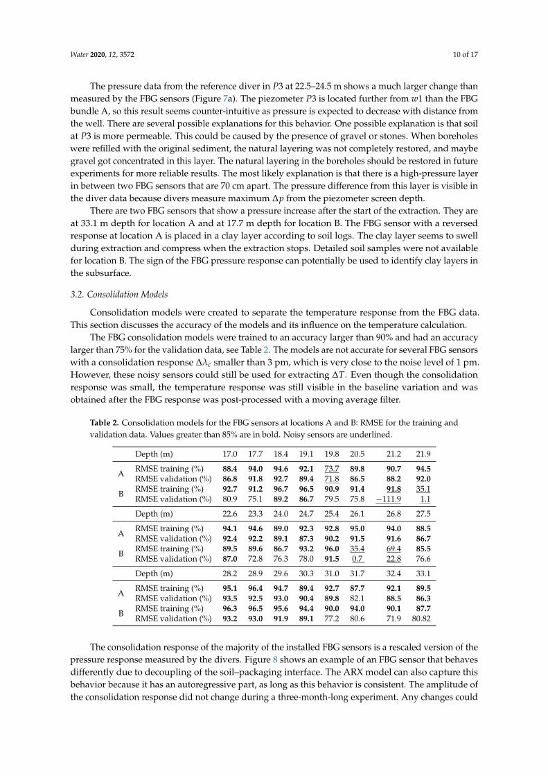
The FBG consolidation models were trained to an accuracy larger than 90% and had an accuracylarger than 75% for the validation data, see Table 2. The models are not accurate for several FBG sensorswith a consolidation response ∆λc smaller than 3 pm, which is very close to the noise level of 1 pm.However, these noisy sensors could still be used for extracting ∆T. Even though the consolidationresponse was small, the temperature response was still visible in the baseline variation and wasobtained after the FBG response was post-processed with a moving average filter.
Table 2. Consolidation models for the FBG sensors at locations A and B: RMSE for the training andvalidation data. Values greater than 85% are in bold. Noisy sensors are underlined.
Depth (m) 17.0 17.7 18.4 19.1 19.8 20.5 21.2 21.9
RMSE training (%) 88.4 94.0 94.6 92.1 73.7 89.8 90.7 94.5A RMSE validation (%) 86.8 91.8 92.7 89.4 71.8 86.5 88.2 92.0
B RMSE training (%) 92.7 91.2 96.7 96.5 90.9 91.4 91.8 35.1RMSE validation (%) 80.9 75.1 89.2 86.7 79.5 75.8 −111.9 1.1
Depth (m) 22.6 23.3 24.0 24.7 25.4 26.1 26.8 27.5
RMSE training (%) 94.1 94.6 89.0 92.3 92.8 95.0 94.0 88.5A RMSE validation (%) 92.4 92.2 89.1 87.3 90.2 91.5 91.6 86.7
B RMSE training (%) 89.5 89.6 86.7 93.2 96.0 35.4 69.4 85.5RMSE validation (%) 87.0 72.8 76.3 78.0 91.5 0.7 22.8 76.6
Depth (m) 28.2 28.9 29.6 30.3 31.0 31.7 32.4 33.1
RMSE training (%) 95.1 96.4 94.7 89.4 92.7 87.7 92.1 89.5A RMSE validation (%) 93.5 92.5 93.0 90.4 89.8 82.1 88.5 86.3
B RMSE training (%) 96.3 96.5 95.6 94.4 90.0 94.0 90.1 87.7RMSE validation (%) 93.2 93.0 91.9 89.1 77.2 80.6 71.9 80.82
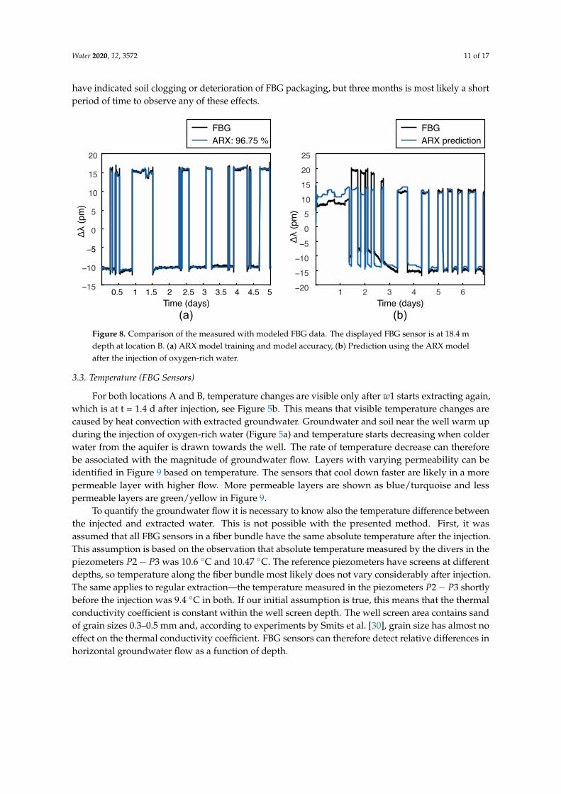
The consolidation response of the majority of the installed FBG sensors is a rescaled version of thepressure response measured by the divers. Figure 8 shows an example of an FBG sensor that behavesdifferently due to decoupling of the soil–packaging interface. The ARX model can also capture thisbehavior because it has an autoregressive part, as long as this behavior is consistent. The amplitude ofthe consolidation response did not change during a three-month-long experiment. Any changes could
Water 2020, 12, 3572 11 of 17
have indicated soil clogging or deterioration of FBG packaging, but three months is most likely a shortperiod of time to observe any of these effects.
−15
−10
−5
0
5
10
15
20
FBG
ARX: 96.75 %
Time (days)
Δλ
(pm
)
FBG
ARX prediction
−20
−15
−10
−5
0
5
10
15
20
25
Δλ
(pm
)
Time (days)
0.5 1 1.5 2 2.5 3 3.5 4 4.5 5 1 2 3 4 5 6
(a) (b)
Figure 8. Comparison of the measured with modeled FBG data. The displayed FBG sensor is at 18.4 mdepth at location B. (a) ARX model training and model accuracy, (b) Prediction using the ARX modelafter the injection of oxygen-rich water.
3.3. Temperature (FBG Sensors)
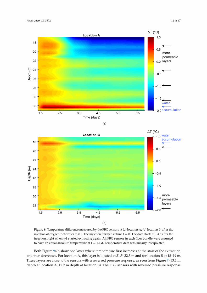
For both locations A and B, temperature changes are visible only after w1 starts extracting again,which is at t = 1.4 d after injection, see Figure 5b. This means that visible temperature changes arecaused by heat convection with extracted groundwater. Groundwater and soil near the well warm upduring the injection of oxygen-rich water (Figure 5a) and temperature starts decreasing when colderwater from the aquifer is drawn towards the well. The rate of temperature decrease can thereforebe associated with the magnitude of groundwater flow. Layers with varying permeability can beidentified in Figure 9 based on temperature. The sensors that cool down faster are likely in a morepermeable layer with higher flow. More permeable layers are shown as blue/turquoise and lesspermeable layers are green/yellow in Figure 9.
To quantify the groundwater flow it is necessary to know also the temperature difference betweenthe injected and extracted water. This is not possible with the presented method. First, it wasassumed that all FBG sensors in a fiber bundle have the same absolute temperature after the injection.This assumption is based on the observation that absolute temperature measured by the divers in thepiezometers P2 − P3 was 10.6 ◦C and 10.47 ◦C. The reference piezometers have screens at differentdepths, so temperature along the fiber bundle most likely does not vary considerably after injection.The same applies to regular extraction—the temperature measured in the piezometers P2 − P3 shortlybefore the injection was 9.4 ◦C in both. If our initial assumption is true, this means that the thermalconductivity coefficient is constant within the well screen depth. The well screen area contains sandof grain sizes 0.3–0.5 mm and, according to experiments by Smits et al. [30], grain size has almost noeffect on the thermal conductivity coefficient. FBG sensors can therefore detect relative differences inhorizontal groundwater flow as a function of depth.
Water 2020, 12, 3572 12 of 17
32
30
28
26
24
22
20
18
De
pth
(m
)
Time (days)
−2.0
−1.5
−1.0
−0.5
0.0
0.5
1.0
ΔT (°C)
more
permeable
layers
water
1.5 2.5 3.5 4.5 5.5 6.5
Location A
accumulation
(a)
more
permeable
layers
De
pth
(m
)
32
30
28
26
24
22
20
18
Time (days)
−2.0
−1.5
−1.0
−0.5
0.0
0.5
1.0
ΔT (°C)
1.5 2.5 3.5 4.5 5.5 6.5
Location B water
accumulation
(b)
Figure 9. Temperature difference measured by the FBG sensors at (a) location A, (b) location B, after theinjection of oxygen-rich water to w1. The injection finished at time t = 0. The data starts at 1.4 d after theinjection, right when w1 started extracting again. All FBG sensors in each fiber bundle were assumedto have an equal absolute temperature at t = 1.4 d. Temperature data was linearly interpolated.
Both Figure 9a,b show one layer where temperature first increases at the start of the extractionand then decreases. For location A, this layer is located at 31.5–32.5 m and for location B at 18–19 m.These layers are close to the sensors with a reversed pressure response, as seen from Figure 7 (33.1 mdepth at location A, 17.7 m depth at location B). The FBG sensors with reversed pressure response
Water 2020, 12, 3572 13 of 17
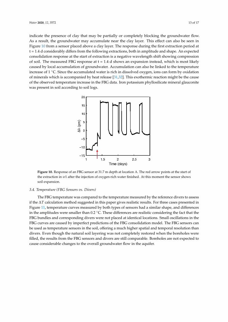
indicate the presence of clay that may be partially or completely blocking the groundwater flow.As a result, the groundwater may accumulate near the clay layer. This effect can also be seen inFigure 10 from a sensor placed above a clay layer. The response during the first extraction period att = 1.4 d considerably differs from the following extractions, both in amplitude and shape. An expectedconsolidation response at the start of extraction is a negative wavelength shift showing compressionof soil. The measured FBG response at t = 1.4 d shows an expansion instead, which is most likelycaused by local accumulation of groundwater. Accumulation can also be linked to the temperatureincrease of 1 ◦C. Since the accumulated water is rich in dissolved oxygen, ions can form by oxidationof minerals which is accompanied by heat release [31,32]. This exothermic reaction might be the causeof the observed temperature increase in the FBG data. Iron potassium phyllosilicate mineral glauconitewas present in soil according to soil logs.
Figure 10. Response of an FBG sensor at 31.7 m depth at location A. The red arrow points at the start ofthe extraction in w1 after the injection of oxygen-rich water finished. At this moment the sensor showssoil expansion.
3.4. Temperature (FBG Sensors vs. Divers)
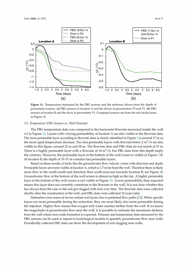
The FBG temperature was compared to the temperature measured by the reference divers to assessif the ∆T calculation method suggested in this paper gives realistic results. For three cases presented inFigure 11, temperature curves measured by both types of sensors had a similar shape, and differencesin the amplitudes were smaller than 0.2 ◦C. These differences are realistic considering the fact that theFBG bundles and corresponding divers were not placed at identical locations. Small oscillations in theFBG curves are caused by imperfect predictions of the FBG consolidation model. The FBG sensors canbe used as temperature sensors in the soil, offering a much higher spatial and temporal resolution thandivers. Even though the natural soil layering was not completely restored when the boreholes werefilled, the results from the FBG sensors and divers are still comparable. Boreholes are not expected tocause considerable changes to the overall groundwater flow in the aquifer.
Water 2020, 12, 3572 14 of 17
1.5 2 2.5 3 3.5 4 4.5 5 5.5 6 6.5
Time (days) Time (days)
−1.4
−1.2
−0.8
−0.6
−0.4
−0.2
0
0.2
T(°
C)
Location A
FBG 18.8±1 m
Diver in P2
FBG 23.5±1 m
Diver in P3
FBG 17.8±1 m
and 23.5±1 m
Diver in P1
−0.6
−0.5
−0.4
−0.3
−0.2
−0.1
0
0.1Location B
T( °
C)
1.5 2 2.5 3 3.5 4 4.5 5 5.5 6 6.5
(a) (b)
−1
Figure 11. Temperature measured by the FBG sensors and the reference divers from the depth ofpiezometer screens. (a) FBG sensors at location A and the divers in piezometers P2 and P3. (b) FBGsensors at location B and the diver in piezometer P1. Compared sensors are from the red-circled areasin Figure 1b.
3.5. Temperature (FBG Sensors vs. Well Flowrate)
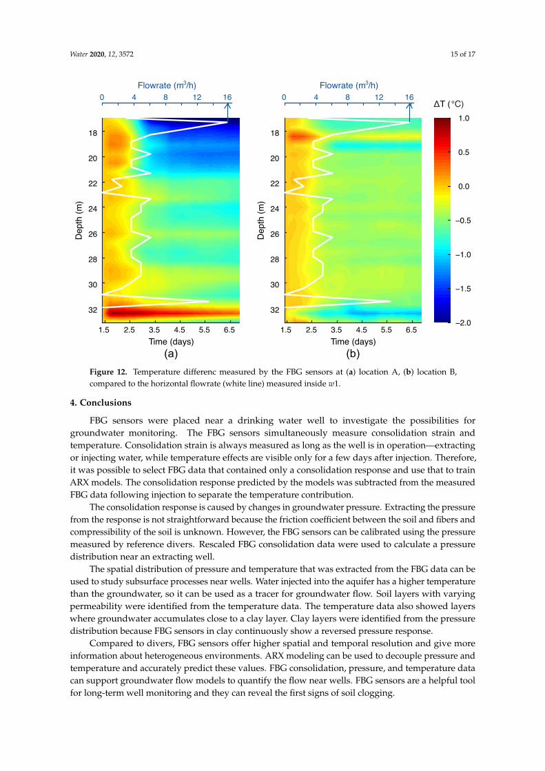
The FBG temperature data was compared to the horizontal flowrate measured inside the wellw1 in Figure 12. Layers with varying permeability at location A are also visible in the flowrate data.The most permeable layer according to flowrate data is clearly identified in Figure 12a around 17 m asthe most rapid temperature decrease. Two less permeable layers with flowrate below 2 m3/h are alsovisible in this figure, around 22 m and 30 m. The flowrate data and FBG data do not match at 31 m.There is a highly permeable layer with a flowrate of 14 m3/h, but FBG data from this depth implythe contrary. However, the permeable layer at the bottom of the well screen is visible in Figure 12b.At location B, the depth of 19–31 m contains less permeable layers.
Based on these results, it looks like the groundwater flow velocity varies with direction and depth.Permeable layers are more visible at location A, which is 1.7 m far from the well. Therefore there is likelymore flow in the south-south-east direction than south-east-east towards location B, see Figure 1b.Groundwater flow at the bottom of the well screen is almost as high as the top. A highly permeablelayer at the bottom of the well screen is not visible in Figure 12. Lower permeability than expectedmeans this layer does not currently contribute to the flowrate in the well. It is not clear whether thishas always been the case or the soil got clogged with iron over time. The flowrate data were collectedshortly after the construction of the well, and FBG data were collected 19 years later.
Subsurface iron removal favors certain soil layers due to preferred flow paths [24]. When specificlayers are more permeable during the extraction, they are most likely also more permeable duringthe injection. Higher flow means that oxygen-rich water reaches further from the well. If we knowthe magnitude of groundwater flow near the well, it is possible to estimate the maximum distancefrom the well where iron oxide formation is expected. Pressure and temperature data measured by theFBG sensors can be used as inputs to hydrological models to quantify groundwater flow near wells.Periodically collected FBG data can show the development of soil clogging near wells.
Water 2020, 12, 3572 15 of 17
1.5 2.5 3.5 4.5 5.5 6.5
32
30
28
26
24
22
20
18
De
pth
(m
)
Time (days)
Flowrate (m /h)3
0 4 8 12 16
1.5 2.5 3.5 4.5 5.5 6.5
32
30
28
26
24
22
20
18
De
pth
(m
)
Time (days)
Flowrate (m /h)3
0 4 8 12 16
−2.0
−1.5
−1.0
−0.5
0.0
0.5
1.0
ΔT (°C)
(a) (b)
Figure 12. Temperature differenc measured by the FBG sensors at (a) location A, (b) location B,compared to the horizontal flowrate (white line) measured inside w1.
4. Conclusions
FBG sensors were placed near a drinking water well to investigate the possibilities forgroundwater monitoring. The FBG sensors simultaneously measure consolidation strain andtemperature. Consolidation strain is always measured as long as the well is in operation—extractingor injecting water, while temperature effects are visible only for a few days after injection. Therefore,it was possible to select FBG data that contained only a consolidation response and use that to trainARX models. The consolidation response predicted by the models was subtracted from the measuredFBG data following injection to separate the temperature contribution.
The consolidation response is caused by changes in groundwater pressure. Extracting the pressurefrom the response is not straightforward because the friction coefficient between the soil and fibers andcompressibility of the soil is unknown. However, the FBG sensors can be calibrated using the pressuremeasured by reference divers. Rescaled FBG consolidation data were used to calculate a pressuredistribution near an extracting well.
The spatial distribution of pressure and temperature that was extracted from the FBG data can beused to study subsurface processes near wells. Water injected into the aquifer has a higher temperaturethan the groundwater, so it can be used as a tracer for groundwater flow. Soil layers with varyingpermeability were identified from the temperature data. The temperature data also showed layerswhere groundwater accumulates close to a clay layer. Clay layers were identified from the pressuredistribution because FBG sensors in clay continuously show a reversed pressure response.
Compared to divers, FBG sensors offer higher spatial and temporal resolution and give moreinformation about heterogeneous environments. ARX modeling can be used to decouple pressure andtemperature and accurately predict these values. FBG consolidation, pressure, and temperature datacan support groundwater flow models to quantify the flow near wells. FBG sensors are a helpful toolfor long-term well monitoring and they can reveal the first signs of soil clogging.
Water 2020, 12, 3572 16 of 17
Author Contributions: Conceptualization: S.D., R.M.W., H.L.O., methodology: S.D., R.M.W., H.L.O., software:S.D., validation: S.D., K.J.K., formal analysis: S.D., investigation: S.D., resources: S.D., data curation: S.D.,writing—original draft preparation: S.D., writing—review and editing: S.D., R.M.W., K.J.K., H.L.O., visualization:S.D., supervision: R.M.W., H.L.O. All authors have read and agreed to the published version of the manuscript.
Funding: Wetsus is co-funded by the Dutch Ministry of Economic Affairs and Ministry of Infrastructure andEnvironment, the European Union Regional Development Fund, the Province of Fryslân, and the NorthernNetherlands Provinces. This research received funding from the European Union’s Horizon 2020 research andinnovation programme under the Marie Skłodowska-Curie grant agreement No. 665874.
Acknowledgments: This work was performed in the cooperation framework of Wetsus, European Centre ofExcellence for Sustainable Water Technology (www.wetsus.nl). We are grateful to the participants of the researchtheme “Groundwater technology” for fruitful discussions and financial support. The authors also thank CasparV.C. Geelen for advice on data proceessing.
Conflicts of Interest: The authors declare no conflict of interest. The funders had a role in the decision to publishthe results.
References
1. Boak, R. Technical Review: Practical Guidelines for Test Pumping in Water Wells; Technical Report;International Committee of the Red Cross: Geneva, Switzerland, 2011.
2. Chen, X.; Goeke, J.; Ayers, J.F.; Summerside, S. Observation well network design for pumping tests inunconfined aquifers. J. Am. Water Resour. Assoc. 2003, 39, 17–32. [CrossRef]
3. Walton, W. Groundwater Pumping Tests; Taylor & Francis: Abingdon-on-Thames, UK, 1990.4. van Beek, C.K. Cause and Prevention of Clogging of Wells Abstracting Groundwater from Unconsolidated
Aquifers. Ph.D. Thesis, VU Amsterdam, Amsterdam, The Netherlands, 2015. [CrossRef]5. Harou, J.J.; Lund, J.R. Ending groundwater overdraft in hydrologic-economic systems. Hydrogeol. J. 2008,
16, 1039–1055. [CrossRef]6. Du, Z.; Ge, L.; Ng, A.H.M.; Zhu, Q.; Zhang, Q.; Kuang, J.; Dong, Y. Long-term subsidence in Mexico City
from 2004 to 2018 revealed by five synthetic aperture radar sensors. Land Degrad. Dev. 2019, 30, 1785–1801.[CrossRef]
7. Loáiciga, H.A. Consolidation Settlement in Aquifers Caused by Pumping. J. Geotech. Geoenviron. Eng. 2012,139, 1191–1204. [CrossRef]
8. Shen, S.L.; Xu, Y.S. Numerical evaluation of land subsidence induced by groundwater pumping in Shanghai.Can. Geotech. J. 2011, 48, 1378–1392. [CrossRef]
9. Lienau, P.J. Data Acquisition for Low-Temperature Geothermal Well Tests and Long-Term Monitoring;Technical Report; U.S. Department of Energy: Idaho Falls, ID, USA, 1992. [CrossRef]
10. Paillet, F. Borehole flowmeter applications in irregular and large-diameter boreholes. J. Appl. Geophys. 2004,55, 39–59. [CrossRef]
11. Zhou, Y.; Li, W. A review of regional groundwater flow modeling. Geosci. Front. 2011, 2, 205–214. [CrossRef]12. Selker, J.S.; Thévenaz, L.; Huwald, H.; Mallet, A.; Luxemburg, W.; van de Giesen, N.; Stejskal, M.;
Zeman, J.; Westhoff, M.; Parlange, M.B. Distributed fiber-optic temperature sensing for hydrologic systems.Water Resour. Res. 2006, 42. [CrossRef]
13. Campanella, C.E.; Cuccovillo, A.; Campanella, C.; Yurt, A.; Passaro, V.M. Fibre Bragg Grating based strainsensors: Review of technology and applications. Sensors 2018, 18, 3115. [CrossRef]
14. Huang, J.Y.; Roosbroeck, J.V.; Vlekken, J.; Daerden, E.; Martinez, A.B.; Geernaert, T.; Berghmans, F.;Hoe, B.V.; Lindner, E.; Caucheteur, C. Packaged FBG based optical fiber sensor for simultaneous pressureand temperature monitoring. In Fiber Optic Sensors and Applications XV; Mendez, A., Baldwin, C.S.,Du, H.H., Eds.; International Society for Optics and Photonics, SPIE: Bellingham, WA, USA, 2018;Volume 10654, pp. 93–99. [CrossRef]
15. Ameen, O.F.; Younus, M.H.; Aziz, M.S.; Azmi, A.I.; Ibrahim, R.K.R.; Ghoshal, S.K.; Raja Ibrahim, R.K.;Ghoshal, S.K. Graphene diaphragm integrated FBG sensors for simultaneous measurement of water leveland temperature. Sens. Actuators A Phys. 2016, 252, 225–232. [CrossRef]
16. Dinia, L.; Mangini, F.; Muzi, M.; Frezza, F. FBG multifunctional pH sensor-monitoring the pH rain in culturalheritage. Acta IMEKO 2018, 7, 24–30. [CrossRef]
Water 2020, 12, 3572 17 of 17
17. Bellas, M.; Voulgaridis, G. Study of the major landslide at the community of Ropoto, Central Greece,mitigation and FBG early warning system design. Innov. Infrastruct. Solut. 2018, 3, 1–14. [CrossRef]
18. Wang, M.; Chen, J.; Wei, H.; Song, B.; Xiao, W. Investigation on seismic damage model test of a high concretegravity dam based on application of FBG strain sensor. Complexity 2019, 2019. [CrossRef]
19. Monsberger, C.; Klug, F.; Lienhart, W. Performance assessment of a fiber Bragg grating sensor networkinside a hydro power dam using optical backscatter reflectometry. In Fiber Optic Sensors and ApplicationsXIV; International Society for Optics and Photonics: Bellingham, WA, USA, 2017; Volume 10208, p. 102080R.[CrossRef]
20. Qiao, X.; Shao, Z.; Bao, W.; Rong, Q. Fiber Bragg Grating Sensors for the Oil Industry. Sensors 2017, 17, 429.[CrossRef] [PubMed]
21. Alemohammad, H.; Liang, R.; Yilman, D.; Azhari, A.; Mathers, K.; Chang, C.; Chan, B.; Pope, M.A. Fiber opticsensors for harsh environments: Environmental, hydrogeological, and chemical sensing applications.In Proceedings of the 26th International Conference on Optical Fiber Sensors, Lausanne, Switzerland,24–28 September 2018. [CrossRef]
22. Gu, K.; Shi, B.; Liu, C.; Jiang, H.; Li, T.; Wu, J. Investigation of land subsidence with the combination ofdistributed fiber optic sensing techniques and microstructure analysis of soils. Eng. Geol. 2018, 240, 34–47.[CrossRef]
23. Wu, J.; Jiang, H.; Su, J.; Shi, B.; Jiang, Y.; Gu, K. Application of distributed fiber optic sensing technique inland subsidence monitoring. J. Civ. Struct. Health Monit. 2015, 5, 587–597. [CrossRef]
24. Van Halem, D.; de Vet, W.; Verberk, J.; Amy, G.; van Dijk, H. Characterization of accumulated precipitatesduring subsurface iron removal. Appl. Geochem. 2011, 26, 116–124. [CrossRef]
25. Drusová, S.; Wagterveld, R.M.; Wexler, A.D.; Offerhaus, H.L. Dynamic consolidation measurements in awell field using fiber Bragg grating sensors. Sensors 2019, 19, 4403. [CrossRef]
26. Zanotti, C.; Rotiroti, M.; Sterlacchini, S.; Cappellini, G.; Fumagalli, L.; Stefania, G.A.; Nannucci, M.S.; Leoni,B.; Bonomi, T. Choosing between linear and nonlinear models and avoiding overfitting for short and longterm groundwater level forecasting in a linear system. J. Hydrol. 2019, 578, 124015. [CrossRef]
27. Varouchakis Emmanouil, A. Modeling of temporal groundwater level variations based on a Kalman filteradaptation algorithm with exogenous inputs. J. Hydroinf. 2017, 19, 191–206. [CrossRef]
28. Keesman, K.J. System Identification An Introduction; Springer: London, UK, 2019; Volume 53, pp. 1689–1699.[CrossRef]
29. Kashyap, R. Fiber Bragg Gratings; Electronics & Electrical; Elsevier Science: Philadelphia, PA, USA, 1999.30. Smits, K.M.; Sakaki, T.; Limsuwat, A.; Illangasekare, T.H. Thermal Conductivity of Sands under Varying
Moisture and Porosity in Drainage–Wetting Cycles. Vadose Zone J. 2010, 9, 172. [CrossRef]31. Dos Santos, E.C.; De Mendonça Silva, J.C.; Duarte, H.A. Pyrite Oxidation Mechanism by Oxygen in Aqueous
Medium. J. Phys. Chem. C 2016, 120, 2760–2768. [CrossRef]32. Drusová, S.; Offerhaus, H.L.; Wagterveld, R.M.; Keesman, K.J. Simultaneous temperature and consolidation
sensing near drinking water wells using fiber-optic sensors. 4TU.ResearchData Collect. 2020. [CrossRef]
Publisher’s Note: MDPI stays neutral with regard to jurisdictional claims in published maps and institutionalaffiliations.
© 2020 by the authors. Licensee MDPI, Basel, Switzerland. This article is an open accessarticle distributed under the terms and conditions of the Creative Commons Attribution(CC BY) license (http://creativecommons.org/licenses/by/4.0/).