Embed Size (px)
Citation preview

Television demand for the Tour de France: the importance of outcome uncertainty,
patriotism and doping
Daam Van Reeth
HUB RESEARCH PAPERS 2011/15
ECONOMICS & MANAGEMENT SEPTEMBER 2011

1
Television demand for the Tour de France: the importance of outcome uncertainty, patriotism and doping
Daam Van Reeth
Hogeschool-Universiteit Brussel, Campus Economische Hogeschool, Stormstraat 2, B-1000 Brussels, [email protected]
Abstract
This paper analyzes demand for televised cycling races. Using data for 296 Tour
de France broadcasts from 1997 until 2010, average and peak TV audience per
stage is estimated by an OLS regression model. A first set of independent
variables measures the importance of stage scheduling and includes variables that
define the stage type and stage date. These variables are defined ex ante by the
race organiser and can therefore be controlled to influence viewing. A second set
of variables consists of stage features not under the control of the race organiser.
These variables measure the importance of outcome uncertainty, patriotism,
doping and weather conditions. Our findings suggest that viewership of televised
cycling is largely determined by stage characteristics. Only on a much smaller
scale are viewing habits driven by race developments. The study supports the idea
that a well-chosen profile of stages is crucial when trying to maximize Tour de
France TV viewership.
Key words: Tour de France, TV demand, outcome uncertainty, doping,
patriotism
1. INTRODUCTION
The Tour de France is the most important cycling race in the world. The
three-week race takes place in July each year and captures the interest of tens of
millions of cycling fans every day. Alongside the cobblestones classics Paris-
Roubaix and the Ronde van Vlaanderen it is the only cycling race to get

2
worldwide live coverage. According to the race organiser ASO1, global TV
audience for the 21 stages amounts to almost 1 billion spectators. Many fans also
watch the race from the roadside. The live audience along the Tour de France
route during the whole event is estimated to be around 15 million
(www.letour.fr). The significant media exposure the race offers motivates cycling
teams to line up their best riders. Although an analysis of what drives Tour de
France viewership is therefore clearly appropriate, to our knowledge there has
been no detailed empirical study of Tour de France audience yet, a gap in the
literature which this article wants to address.
The paper investigates to what extent stage scheduling and race features
like outcome uncertainty, patriotism, doping and the presence of substitute goods
influence live Tour de France TV viewing. As a case study, viewing data for
Flanders, the Northern part of Belgium, were used. Although one of the smaller
European TV markets, the choice of Flanders is highly relevant when studying
road cycling. In 2009 almost 150 cycling races were broadcast over 120 different
days on Flemish television, numbers no other country or region can match. With
about 8% of its population tuning in daily, Flanders also has the highest Tour de
France TV ratings in the world, followed at a distance by Denmark and France
(ViewerTrack 2010). The television popularity of cycling in Flanders is no
surprise. Due to its established heritage in the sport, the region is often described
as "the heart of cycling". This heritage is also reflected in the fact that in many
top cycling teams former Belgian cyclists play a major role. Alberto Contador,
Lance Armstrong, Jan Ullrich and Greg Lemond all won the Tour de France
under the guidance of a Flemish directeur sportif2.
The rest of the paper proceeds as follows. In section 2 we present a
literature survey on TV demand for sport. The Tour de France and its fruitful
relationship with television is explained in section 3. Section 4 describes the data
and the methodology. The empirical results are discussed in section 5.
Conclusions then follow together with a remark on some future research
opportunities.

3
2. LITERATURE ON TV DEMAND FOR SPORT
Empirical studies on sports events demand have focused heavily on live
attendance. The attendance demand for sports events is therefore extremely well
researched. In their survey, Garcia & Rodriguez (2009) list 81 empirical studies
on sports attendance, most of them analyzing popular sports like baseball or
soccer. But for road cycling this attendance approach is inadequate. The sport is
taking place on public roads and there is no host team playing in a home stadium.
TV viewership and not live attendance is therefore the more relevant measure to
use when studying demand for road cycling.
The literature on television audience demand is still relatively
underdeveloped compared to the literature analysing live attendance. The
historically-based research focus on live attendance resulted in much of the initial
research on TV demand for sports, analysing the impact of live broadcasting on
game attendance rather than analysing the actual TV audiences. Over the years,
the so-called crowding-out effect of television on attendance has been studied for
sports as diverse as American football (Kaemper & Pacey (1986), Fizel & Bennett
(1989), Putsis & Sen (2000)), basketball (Zhang & Smith (1997)), rugby
(Baimbridge et al. (1995) and Carmichael et al. (1999)) and soccer (Kuypers
(1996), Baimbridge, Cameron & Dawson (1996), Czarnitzki & Stadtmann (2002),
Forrest, Simmons & Szymanski (2004) and Allan & Roy (2008)). The studies
show some mixed evidence as to whether there is a significant impact of
broadcasting on attendance. Baimbridge et al. (1995) find a 25% decline in
stadium attendance in the case of rugby while Kuypers (1996) found no
significant effect for the English Premier Football League. Czarnitzki &
Stadtmann (2002) even estimated a positive effect when modelling attendance in
German football. Because, given the absence of a home stadium, a study of the
crowding-out effect is irrelevant in the case of cycling, we will not discuss this
line of research any further.
A second important subject that sports economists analysing TV demand
have concentrated their attention on is the impact of outcome uncertainty on TV

4
viewership. Although there had been some previous research in this field3, this
line of research has only recently witnessed a significant boost in interest,
kickstarted by the seminal article of Forrest, Simmons & Buraimo (2005) on what
they call the couch potato audience. Based on a model that estimates the determinants
of audience figures, Forrest et al. (2005) conclude that in the English Premier
Football League “outcome uncertainty is a significant determinant of audience size, but the
magnitude of its impact appears to be modest.” The authors also took a look at the
supply side of the TV market by modelling the broadcaster's choice of games to
be screened.4 They find some evidence that both broadcaster and audience
favour matches expected to be close.
Their work inspired similar studies on other European football leagues.
For the Spanish first division Garcia & Rodriguez (2006) report that the ex ante
attractiveness of a match is the main determinant of the size of the audience.
They also find a strong seasonal component in the evolution of the size of the
audience within the football season. Also Buraimo & Simmons (2007) analyse
Spanish football and conclude that "unlike their stadium counterparts, who have a
preference for outcomes which favour their home team, TV audiences overwhelmingly prefer close
matches than ones in which the outcomes are more predictable." The Italian first division
was studied by Di Domizio (2010). He shows that more then 90% of the
variability concerning TV audiences can be explained net of uncertainty factors.
Variables associated with the closeness of the match increase the goodness of fit,
but are not crucial in determining the TV share.
Other European authors analysed TV football audiences from a different
point of view. In a novel approach, Alavy, Gaskell, Leach & Szymanski (2010)
analyze minute to minute intragame viewership for English League football
matches and find that “although uncertainty matters, it is the progression of the match which
drives viewership and as a draw looks increasingly likely, viewers are likely to switch channels.”
Based on a comparison between two Scandinavian football leagues, Johnsen &
Solvoll (2007) report that viewers have different motives for watching games on a
public service broadcaster to those watching on a private channel. For a private
channel content (the types of games shown) is decisive, while for a public service

5
broadcaster timing (scheduling strategies) is everything. Nüesch & Franck (2009)
present evidence of patriotism in TV viewership by examining data for
international football games between countries. They show that both the
expected game quality based on the proven playing strength of the teams and
levels of patriotism strongly predict the TV figures.
Also American sports economists have recently studied TV audiences in
relation to outcome uncertainty. Berkowitz, Depken & Wilson (2010) compare
TV viewership and attendance in NASCAR racing and conclude that "with greater
uncertainty, fan interest reflected in attendance and viewership increases. With less competitive
balance, fan interest in TV viewership falls but attendance is not influenced." Biner (2009)
studies American Football and reports that “while stadium attendance is determined by
home team’s dominance, TV ratings are determined mostly by close games with possibly strong
teams playing each other”.
Finally we briefly point to the analysis of spectator motives for watching
sport on television as a third line of research in television audience demand. Fink
& Parker (2009) and Solberg & Hammervold (2008) present evidence that
outcome uncertainty is not as important for peoples' interest in sport as the
literature in sports economics has argued in the past.
3. TELEVISION AND THE TOUR DE FRANCE: A PERFECT MATCH
TV coverage of the Tour de France started shortly after World War II
with the first live broadcast of the Tour’s conclusion at the Parc des Princes in
Paris in 1948. Previously, images of the Tour de France had only been shown on
cinema newsreels a couple of days after the event took place. The success of the
1948 live transmission prompted French television to schedule a daily evening
news program. During the 1950s the popularity of the Tour de France news
programs grew resulting in the first live coverage from within the race in 1958 on
the legendary col d’Aubisque. French television began to pay for the right to
cover the race in 1960. That year, nine hours and twenty minutes of race
coverage was provided, including four hours of live coverage (Thompson, 2008).

6
In the following decades, television coverage expanded in duration and
scope. European countries like Belgium, the Netherlands and Italy started live
transmission in the 1960s and 1970s. The race was broadcast for the first time in
the United States in 1979 and in Japan in 1985 (Thompson, 2008). Australia,
China and Latin American countries soon followed, making the Tour de France
one of the most viewed multiday sports events.5 In 2011 TV channels provided
coverage of the Tour de France in 190 countries including live coverage in 60,
twice as many as in 2000 (www.letour.fr). Decisive stages attract between 40 and
50 million TV viewers worldwide (ViewerTrack 2010), offering sponsors of
cycling teams valuable exposure to a large audience.
Several elements make the Tour de France and television such a perfect
match. Firstly, unlike many other sports, road cycling can only be understood
well through access to the media. While a spectator at a soccer match might not
get the best view of the action, he would at least know the score. With cycling,
you can only appreciate the day's racing by watching it on television. Note that
historically there has always been an important link between the media and road
cycling. Indeed, many big races were originally created as a promotional tool.
Both the Tour de France and the Giro d’Italia were at first just a means to
increase newspaper sales for the organizing media behind the race, l’Auto in
France and La Gazzetta dello Sport in Italy. In fact, in recent decades television
has largely taken over the newspapers' primary role of telling the heroic story of
the Tour de France.
Secondly, road cycling is an ideal means to promote tourism. Although at
Wimbledon or in a Champion's League final you also get some obligatory
promotional city overview shots, there is no connection between the sport and
the images shown. With road cycling this is different. Cyclists not only compete
with each other, they also have to overcome the obstacles the stage route
imposes. To guarantee the best possible coverage of how the race develops
helicopters and motorbikes carrying cameramen have to follow the cyclists along
the stage route. Road cycling broadcasts thus offer a harmonious mix of live
sport images and complementary roadside showings of the scenery. With the

7
exception of sports like city marathon running or the triathlon, this natural mix
of images is present in almost no other sport and it makes road cycling one of the
most watched sports by non-sports fans. It offers places along the Tour de
France route invaluable exposure to a broad audience.6 Just as the 2008 Beijing
Olympic Road Race was a well designed promotional clip for the rich tourist
value of the Beijing region, the Tour de France represents a yearly showcase for
the cities, towns, villages and landscapes of France. For this reason, in
partnership with the French tourism agencies ASO also provides an extensive
stage per stage tourist guide which sports journalists can use in their daily stage
commentaries.
Thirdly, road cycling is not subject to many technical rules or complex
game regulations. Basically the first rider to cross the finish wins the stage. The
absence of important viewing barriers makes the sport accessible to a large
audience and stimulates social and family watching.
Fourthly, road cycling is not a prime time evening sport like, for instance,
football. Consequently, cycling races are fairly easy to fit into the TV schedule.
To a European broadcaster the afternoon Tour de France broadcasts are a
welcome and well-watched alternative to the reruns of old TV programs that
often fill the afternoon TV slots, especially in the dull summer period.
4. MODELLING TV DEMAND FOR TOUR DE FRANCE STAGES
The Tour de France has a long and heroic history of over 100 years. The
race lasts for three weeks, counting 21 stages that differ in length and route. The
cyclist who has taken the least time overall to cover the course wins. Three types
of stage exist: flat stages, mountain stages and time trial stages. Flat stages are
easy to ride and are likely to end in a bunch sprint. They are of almost no
importance to the overall Tour de France win although occasionally top
favourites suffer time losses when crashes or windy conditions result in splits in
the peloton7. When riders have to cycle up steep mountain passes, the race
becomes much harder and usually large time differences between riders are

8
created. Mountain stages are therefore crucial to the overall Tour de France result
and attract a much larger audience. While flat stages and mountain stages are
raced collectively, the peloton starting en mass together, time trial stages are
ridden individually or, sometimes, in teams. Cyclists start at equal time intervals,
usually one or two minutes apart. The absence of clear man-to-man action makes
time trial stages less spectacular to the TV public8, but as they might result in
significant time differences between riders, time trial stages are very important to
the overall Tour de France result too.
The overall time classification is the most prestigious classification to win,
the leader wearing the famous yellow jersey.9 But there are other competitions of
importance too. The points classification, awarded with a green jersey,
determines the best sprinter, the rider who is best capable of winning the bunch
sprint when the whole peloton is still together at the end of a stage. A polka-dot
jersey is worn by the king of the mountains, the leader in the classification for the
best climber, while the best young rider receives a distinctive plain white jersey.
Only cyclists under 25 years of age are eligible for this competition. Next to these
individual classifications, there is also a team classification based on the time of
each team's best three riders in every stage. Not all participating teams have a
strong enough contender for an overall classification. These teams might focus
on individual stage victories instead. But with 22 teams participating and only 5
overall classifications at stake, the stage victories are also hard-fought. In fact,
usually about half of the teams leave the Tour de France empty-handed. The mix
of different stages with multiple success opportunities makes all stages, including
the flat ones, interesting for a large TV audience.
The dependent variables
Different viewership measures are used in sports literature. Some studies
analyse a television rating, which is the percentage of viewers watching the
program out of a potential audience. Other studies focus on the average number
of people watching a program. When the potential audience remains about
constant both measures, of course, lead to the same results. A third viewership

9
measure is the peak audience. Although not yet used in sports literature, we argue
that especially in cycling, for at least for two reasons, analysing the peak audience
is relevant. Firstly, in many sports depending on the progress of the game the
number of viewers more or less remains constant or even decreases. In a cycling
race, however, viewership increases massively towards the conclusion of the race.
Secondly, broadcasts of cycling races differ in length, not only between races but
also between TV channels. Important Tour de France stages are often broadcast
from start to finish, the program sometimes lasting 6 hours or more. Less
spectacular stages usually get coverage of the final 2 or 3 hours only.
Insert figure 1 about here
Figure 1 illustrates the minute-by-minute evolution of the TV audience
for a typical Tour de France broadcast. In the course of the program the
audience grows steadily to 1.5 million, three times the initial audience. While the
peak audience at the end of the race is independent of the length of the program,
the average audience very much depends on this duration. If the TV channel had
opted for a shorter broadcast of only the final hour, the average audience would
have been well in excess of 1.2 million, much more than the now reported
average audience of 941,000. This also shows one has to be careful in comparing
audience figures across countries, especially between cycling-popular countries
with long broadcasts and other countries with much shorter live coverage of
cycling races.
It is safe to assume the average audience mainly reflects the interest on
the part of true cycling fans who prefer to watch every minute of a broadcast.
The peak audience basically gives an idea of the general level of interest in (part
of) a cycling race. This measure therefore better captures the importance of the
occasional, thrill-seeking or 'social' cycling audience watching only the most
relevant part of a cycling race, usually the final kilometres. To analyse a potential
difference in viewing motives between true and occasional cycling fans, in our
analysis both the average audience and the peak audience are used as dependent

10
variables. Note we prefer to use the average audience to a TV-rating because it
delivers a more direct interpretation of the results in terms of people watching
and it allows better comparison with the peak audience figures.
It should be noted that all reported viewership measures underestimate
the real number of people watching a program. This is because official data
account for resident viewership only, excluding for instance group viewership in
pubs and viewership from abroad. In the case of cycling, the TV audience from
abroad is significant. Many Dutch fans, for instance, prefer to watch cycling on
Flemish television because of the professional and well-informed commentary.
These spectators are neither included in the reported Flemish viewership data nor
in the reported Dutch viewership data. Unfortunately, no official data on the
number of foreign spectators for cycling races on Flemish television are
available.10
The independent variables
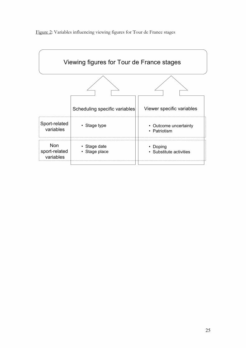
In their analysis of football Johnsen & Solvoll (2007, p. 322) identify two
groups of determinants for TV viewership: scheduling specific factors and
football specific factors. In figure 2 we adapt their model to the case of the Tour
de France and assume that viewing figures are determined mainly by two sorts of
independent variables: scheduling specific variables and viewer specific variables.
Insert figure 2 about here
As early as October, the profile of next year's Tour de France is
announced in detail. Day-to-day information on all the individual stages is made
public, including a description of the route from start to finish. In our model 17
scheduling specific dummy variables were included as control variables to
describe all the relevant ex ante stage characteristics that are already known many
months before the race actually takes place.
There are 6 dummy variables to identify the stage type. As described
earlier, stages are labelled as flat stages, mountain stages or time trial stages. We

11
consider the flat stages to be the reference situation and use 3 dummy variables
for defining different types of mountain stages. We make a distinction between
high mountain stages, in the Alps and the Pyrenees or on the Mont Ventoux, and
low mountain stages, for all other mountain stages. Because mountain stages that
finish on a mountain top are more likely to create time gaps between the top
contenders and thus potentially generate more viewer interest, we also created a
dummy for mountain top finishes. The other 3 stage type dummy variables
identify three time trial formats: individual (flat) time trial stages, team time trial
stages and mountain time trial stages.
Not only is the stage type important, the day or date on which the stages
are held matters too. Because to European TV viewers road cycling is an
afternoon sport, stages ridden during the weekend or on a holiday are likely to
attract more viewers than weekday stages. We therefore include another 9
dummy variables to account for these effects. Two dummy variables capture the
expected increase in TV viewership on the Belgian national holiday (July 21) and
on the Flemish national holiday (July 11). Also the first and the final stage of each
Tour de France are identified with a dummy variable. The other 5 day variables
differentiate between stages held on Saturdays, Sundays or weekdays and stages
held in the first, second or third week, the reference situation being a stage held
on a weekday in the first week.
From time to time the Tour de France crosses international borders for
one or more stages, creating an extra interest in the Tour de France in the
country visited. Since in our study we use Flemish/Belgian viewing data, dummy
variables were used to identify stages with a stage start or a stage finish in
Belgium. By using two dummy variables, we are able to differentiate between
stages passing through the Northern part of Belgium, which are likely to have a
significant impact on Flemish viewership data, and stages passing through the
Southern part of Belgium, from which a smaller impact could be expected.
The second set of independent variables is viewer specific. These
variables measure all ad hoc decisions by TV viewers to watch a Tour de France
stage. These decisions are based on sporting factors like outcome uncertainty and

12
patriotism as well as on non-sporting factors like doping and the competition
from alternative activities.
There exists no published research on outcome uncertainty in road
cycling yet. We are convinced this is partly due to the peculiarities of road cycling
that make a statistical analysis less straightforward. As a start, great care has to be
taken in judging time differences or stage results when looking for evidence of
outcome uncertainty in cycling. Two examples illustrate the point. First, part of
Armstrong's tactics in winning the Tour de France was "offering" the yellow
jersey for a couple of days to another team to reduce pressure on his own team.
This was done by deliberately losing time to a group of riders not strong enough
to compete for the overall Tour de France win. To a non-cycling fan Armstrong's
time loss might be indicative of a bad day and stronger than expected
competition, while in reality it just strengthened the hold of the Armstrong team
on the Tour de France peloton, thus in fact reducing outcome uncertainty.
Second, a zero time difference can in the case of a thrilling bunch sprint point to
a great outcome uncertainty. However, in the case of a mountain stage, the same
zero time difference could be the result of a disappointing lack of competition
between the top contenders, fearing each other too much. But not only is it the
case that a correct assessment of time differences is complex, it is also the case
that as a sport road cycling is very different from most other sports. Road cycling
is an individual sport practised in teams in which collusion between competitors
often occurs and is generally accepted as frequently riders may have mutual
interest in working together. Furthermore, there is no home team, as usually
about 20 teams of 6 to 9 riders compete simultaneously during a race. The
absence of a two-team context and the presence of results-distorting strategic and
collusive decisions by teams makes defining and measuring outcome uncertainty
in road cycling a complicated job.
Three outcome uncertainty variables are included in the model. A first
variable captures the importance of single Tour de France stages to the overall
Tour de France win by using a dummy variable to identify suspense stages. Time
differences between top riders in mountain stages and time trial stages are usually

13
below two minutes at the finish. Consequently, outcome uncertainty with respect
to the final Tour de France winner is only significant when current time
differences in the overall standings are not too large. Suspense stages are therefore
defined as third week mountain stages or time trial stages where at the start the
time difference between the top two riders was less than 90 seconds. The squared
number of stage victories obtained so far in this year's Tour de France by last
year's Tour de France winner acts as a second outcome uncertainty variable.
When winning several stages, a defending Tour de France winner shows he is
ready to retain his title, thereby reducing outcome uncertainty. This so-called
dominance variable thus measures the impact of a more predictable outcome. In
addition to these two competition-based variables, to account for a potential
superstar effect the comeback of Armstrong in the 2009 and 2010 Tour de
France was measured by including another dummy variable.
A second group of viewer specific variables measures patriotism. Both
the number of Belgian cyclists participating in the Tour de France and their
success are included as variables in the model. Belgian success was defined as stages
in which a Belgian cyclist was wearing a leader's jersey of any sort. Next to these
two general patriotism variables, two rider-specific patriotism variables were
used. As a result of believed cocaine use, Tom Boonen was banned from the
2008 Tour de France. Being the most successful Belgian Tour de France rider in
previous years, this was likely to reduce TV interest. The opposite happened
when the unexpected good overall results of Jurgen Van Den Broeck created
extra interest in the 2010 Tour de France.
Because all stages are broadcast on public television in Belgium, Tour de
France viewership is free. In the absence of a price, the opportunity cost of
watching Tour de France stages on television is mainly related to the competition
for leisure time. Consequently, weather conditions and simultaneous major sports
events, like Wimbledon or the soccer World Cup, may play a role in Tour de
France viewership. To capture the impact of these alternatives, a third group of
viewer specific variables was created. On rainy days people tend to stay inside
and TV viewing is expected to be higher. A second weather variable was based

14
on the outside temperature in the viewing country. Although at first no
straightforward relationship between temperature and Tour de France viewership
could be detected, a more detailed analysis led to a surprising result. As long as
temperature is normal for the time of year, temperature does not affect
viewership. But with extremely high as well as with extremely low temperatures,
viewership increases exponentially. The best fit was obtained by constructing a
variable temperature that was set equal to the squared difference in temperature
from 25 degrees Celsius, only if the temperature difference exceeded 5 degrees
Celsius. For smaller differences, this variable was set equal to zero. The only
major rivalling sports event with Belgian participation during Tour de France
stages is Wimbledon. A dummy variable Wimbledon was included in the model to
measure the effect on Tour de France viewership from a live broadcast of a Kim
Clijsters or Justine Henin Wimbledon tennis match.
It is often argued that doping scandals influence TV viewership for road
cycling negatively. In fact, German public TV claimed the drop in German
vierwership for Tour de France stages was due to the continuous doping
atmosphere that surrounds cycling and therefore decided to stop almost all live
coverage of the Tour de France.11 A dummy variable doping was included in the
model to check whether doping cases really affect Tour de France viewership.
Doping stages were defined as the first stage held after a doping case was
uncovered. We should remark though that it is impossible to measure the impact
of famous doping cases like the 2006 Floyd Landis case or the 2010 Albert
Contador case, because both riders were accused of doping use after the finish of
the Tour de France. The public's reaction to these doping cases can therefore not
be reflected in the reported Tour de France viewing figures.
Insert table 1 about here
In table 1 the independent variables are summarized with the expected
sign. All stage date variables are expected to have a positive sign. Mountain stages
are also expected to stimulate TV viewership, while time trials are assumed to

15
negatively influence the number of viewers. The combined effect of the two, a
mountain time trial stage, is not a priori clear. Also for the stage location variables
we do not have any a priori expectation. Grabbing the rare opportunity to see the
Tour de France live, many potential TV viewers will line up along the Tour de
France route, potentially offsetting the extra viewer interest a local Tour passage
creates. The dominance variable is expected to have a negative sign while
suspense stages and the Armstrong comeback should normally attract extra
viewership. Except for the Boonen-dummy, all patriotism variables are expected
to have a positive sign. Finally, rain and large temperature differences will
normally increase TV audience for Tour de France stages, while Wimbledon
matches involving Belgian players and revelations of new doping cases should
lead to a reduced number of TV viewers.
The data
The dataset consists of 296 Tour de France stages broadcast on Flemish
public television (VRT) from 1997 to 2010. Individual stage data including type
of race and day of race were identified for all stages, using publicly available
information on the Tour de France route. Meteorological data were downloaded
from the website of the Dutch Meteorological Institute (www.kmi.nl). To
measure patriotism and outcome uncertainty official race results available on the
Tour de France website were used (www.letour.fr). The mean value or, in the
case of dummy variables, the frequency of the independent variables is also
summarized in table 1.
Viewership data were collected from the Flemish public broadcasting
company (www.vrt.be). Table 2 lists the most and least watched stages on
Flemish television. The mean average audience is 441,983 ranging from a
minimum of 215,488 for the 2007 opening prologue in Strasbourg to a maximum
of 816,066 for the 2010 stage finishing on the legendary col du Tourmalet. All
top 10 best watched stages are mountain stages of which 8 finish on a mountain
top. The least watched stages include 6 time trial stages including 3 team time
trial stages. The Strasbourg prologue also has the lowest peak audience with

16
about 300,000 viewers only. Surprisingly, the top two peak audience stages are
not mountain stages but the 2005 and 2007 final stages to Paris, each attracting
over 1.2 million viewers.12 The mean peak audience is 702,565.
Insert table 2 about here
5. EMPIRICAL RESULTS
We estimated two equations using ordinary least squares regressions. The
two specifications differ by the dependent variable only, the first specification
using average TV audience and the second using peak audience. In the estimates
28 independent variables are included, resulting in a cases-to-variables ratio just
above the threshold level of 10 recommended by the literature. Scatter plots of
the residuals and an outlier analysis indicated no violation of basic regression
assumptions. Results were also checked for autocorrelation and multicollinearity.
With Durbin-Watson statistics of 1.9 and 1.6 and variance inflation factors in
both equations all below 3, the results were judged sound.
As a first step we estimated average Tour de France audiences with the
separate blocks of variables, as depicted in figure 2. An OLS regression with the
6 stage type dummy variables only explained a surprising 48% of the change in
average audience demand, outperforming other specifications with the 11 stage
date and stage place variables (31%), with the 3 outcome uncertainty variables
(19%) or with the 4 patriotism variables (9%). Scheduling specific variables thus
clearly dominate viewer specific variables when explaining television demand for
Tour de France stages, a result in line with earlier findings for football by Forrest,
Simmons & Buraimo (2005) and Di Domizio (2010).
This observation is particularly relevant to Tour de France race organiser
ASO. Because all of the scheduling specific variables are completely under their
control, manipulation of these variables can stimulate TV viewing figures. To this
end, the ASO does indeed carefully plan important stages as much as possible at
the weekend or, for instance, on the French national holiday (July 14) and avoids

17
scheduling one of the obligatory two rest days on a day with huge viewing
potential. Viewer specific independent variables are theoretically out of the
control of the race organiser. Still, by hyping certain stages, by inviting more
teams or riders from countries with high Tour de France TV ratings or by
stimulating the presence of a superstar, as was the case with the Armstrong
comeback in 2009, even some of these variables are to a certain degree
manipulable.
Table 3 displays the results of our final estimates. The complete model
explains almost 80% of the variation in the average audience and over 70% of the
variation in the peak audience. The difference in explanatory power is
understandable if we take into account the more erratic viewing behaviour of the
occasional Tour de France viewer. Other viewing determinants, more difficult to
model, are probably of greater importance to them than to the avid cycling fan.
Insert table 3 about here
Coefficients in table 3 indicate the change in viewership from the
reference scenario: a flat stage on a weekday during the first week under normal
weather conditions with outcome uncertainty and patriotism variables set equal
to zero. An average audience of about 320,000 viewers and a peak audience of
about 610,000 viewers can be expected in this reference situation.
Mountain stages significantly increase TV audiences, but the effect is
much more important for stages through the Alps and the Pyrenees than for
stages crossing less spectacular mountain ranges. Finishes on a mountain top
increase TV audiences even more, but the importance is smaller than expected.
Individual and team time trial stages affect Tour de France viewership negatively.
We believe the absence of a clear man-to-man battle and the more technical
nature of this type of cycling race is largely responsible for this result. A
mountain time trial stage has no significant viewership impact, the mountainous
nature of the stage partially offsetting the lack of any man-to-man action.
18
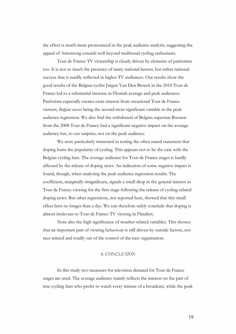
Most of the stage date variables turn out to be strongly significant,
although in the peak audience model this significance is lower for almost all of
the variables. The results indicate that TV interest increases strongly in the
second and third week of the Tour de France, on a national holiday and during
the weekend, the Sunday effect being about twice as important as the Saturday
effect. Unexpectedly, no opening stage effect was detected. This is a puzzling
result because the start of the Tour de France is always much hyped in advance
and the stage is held on a Saturday. The highly significant and extremely large
increase in TV audience for the closing stage to Paris is remarkable too, because
this stage has little or no value from a sporting point of view. The stage basically
boils down to a long parade of the peloton through the streets of Paris. Beauty
shots of Paris are mixed with images of cyclists having fun with each other. Only
in the final kilometres of the stage, the victory is heavily contested, usually
through a bunch sprint finish. In contrast to our a priori expectations, this stage
is highly appreciated by cycling fans and by the general public. We think this may
be the result of the stage being considered by many people as some sort of Tour
de France alternative to an Olympic Games closing ceremony. The show aspect
of the stage and the entertainment value are apparently found to be much more
important than the competition.
A tour passage in the Northern part of Belgium has about the same
considerable impact on TV audiences as the closing stage to Paris. This is an
interesting result because it shows that in contrast to what is the case in many
other sports, there is no crowding-out effect in cycling. Live attendance and TV
viewing are complementary goods instead of substitutes.
After controlling for the stage type and stage date characteristics, it is
possible to test the net impact of outcome uncertainty and patriotism on Tour de
France TV demand. All three outcome uncertainty variables are highly significant
in both specifications of the model. As expected, suspense stages do attract a
large number of extra viewers, while too much dominance reduces the audience.
The Armstrong comeback created the extra interest TV channels hoped for, but
19
the effect is much more pronounced in the peak audience analysis, suggesting the
appeal of Armstrong extends well beyond traditional cycling enthusiasts.
Tour de France TV viewership is clearly driven by elements of patriotism
too. It is not so much the presence of many national heroes, but rather national
success that is readily reflected in higher TV audiences. Our results show the
good results of the Belgian cyclist Jurgen Van Den Broeck in the 2010 Tour de
France led to a substantial increase in Flemish average and peak audiences.
Patriotism especially creates extra interest from occasional Tour de France
viewers, Belgian success being the second most significant variable in the peak
audience regression. We also find the withdrawal of Belgian superstar Boonen
from the 2008 Tour de France had a significant negative impact on the average
audience but, to our surprise, not on the peak audience.
We were particularly interested in testing the often raised statement that
doping hurts the popularity of cycling. This appears not to be the case with the
Belgian cycling fans. The average audience for Tour de France stages is hardly
affected by the release of doping news. An indication of some negative impact is
found, though, when analysing the peak audience regression results. The
coefficient, marginally insignificant, signals a small drop in the general interest in
Tour de France viewing for the first stage following the release of cycling-related
doping news. But other regressions, not reported here, showed that this small
effect lasts no longer than a day. We can therefore safely conclude that doping is
almost irrelevant to Tour de France TV viewing in Flanders.
Note also the high significance of weather-related variables. This showes
that an important part of viewing behaviour is still driven by outside factors, not
race-related and totally out of the control of the race organisation.
6. CONCLUSION
In this study two measures for television demand for Tour de France
stages are used. The average audience mainly reflects the interest on the part of
true cycling fans who prefer to watch every minute of a broadcast, while the peak

20
audience also measures the importance of occasional and social watching. Using a
multiple linear regression model we are able to explain almost 80% of the
variation in average TV audience and over 70% of the variation in peak audience.
Most of the variables have similar levels of significance in both model
specifications.
The OLS regression results indicate that stage characteristics are the main
element in explaining Tour de France TV audience. Almost 65 % of the variation
is determined ex ante by the Tour de France route, as it is designed many months
before the race is actually held. The model shows mountain stages and weekend
stages boost TV interest significantly, while time trial stages lead to an important
drop in TV viewership. The study supports the idea that a well-chosen profile of
stages is crucial when trying to maximize Tour de France TV viewership.
Only on a much smaller scale Tour de France viewership is influenced by
race circumstances and viewer related variables. Stages that are potentially
important to the overall Tour de France win create a significant extra level of
interest, while the defending Tour de France winner dominating the new Tour de
France by winning multiple stages affects viewership negatively, although this
decline in viewership is only of real importance when claiming at least three stage
wins. There is also evidence of a relevant patriotism effect. Good results by
Belgian cyclists are reflected in higher TV ratings. The model indicates superstar
effects are important too. The absence of Belgian superstar Tom Boonen in the
2008 Tour de France because of assumed cocaine abuse reduced viewership
significantly while the Tour comeback of Armstrong in 2009 and 2010 had the
opposite effect. Finally, our results suggest that doping issues are of little
importance to the Flemish cycling fan. The release of cycling-related doping news
doesn't have a significant impact on the average TV audience. There is some
evidence, though, of a slight reduction in the peak audience, pointing to a
temporary small drop in the general interest in cycling because of doping.
This study is the first to use stage level viewership data for televised
cycling. More research is needed to evaluate the robustness of the basic findings
of this paper. As a start, we suggest two future research opportunities. First, a

21
comparative study using viewership data from other countries could question
differences in viewing determinants for cycling across countries, putting for
instance popular belief in French patriotism and a strong German anti-doping
attitude to the test. Second, Tour de France viewership could be compared with
viewing patterns for the other two cycling grand tours: the Giro (Tour of Italy)
and the Vuelta (Tour of Spain). The all-absorbing media attention the Tour de
France generates makes the Giro and the Vuelta look for means of clearly
distinguishing themselves so as to attract a larger TV audience, for instance by
scheduling spectacular stages on steep mountain passes or gravel roads.
The results of this study are relevant to most stakeholders concerned.
Forecasts based on the model can aid the ASO in scheduling a Tour de France
route that maximizes viewing potential and local or national governments in
adequately assessing the promotional impact of televised cycling. It also helps
television companies to properly value a particular broadcast and it is useful to
cycling teams and their sponsors for decisions on team selection and race
strategy. Unfortunately, research in this field is still very much hindered by the
lack of detailed data. We therefore invite television broadcasters and race
organisers to share their viewership data and team up with researchers to further
explore the determinants of TV viewership for cycling.
Acknowledgements I am extremely grateful to Lotte Vermeir, Giovanni Van De Velde and Leon Beerendonk for their assistance in finding the necessary viewership data. I want to thank Mark Corner, Filip Van Den Bossche and the participants in the IASE/ESEA Conferences on Sports Economics (Prague, 2011) and the HUB seminar (Brussels, 2011) for their helpful comments on earlier drafts of this text. 1 Amaury Sport Organisation. ASO also organizes other sports events like Paris-Roubaix (cycling), the Dakar rally (endurance off-road motor sports), the Marathon International de Paris (athletics) and the Open de France (golf). 2 Directeur sportif is the French word for team manager. Many of the specialized terms within cycling are French. 3 According to Buraimo (2008), Pacey & Wickham (1985) were the first to examine the link between game quality and television audience.

22
4 An analysis of the supply side is irrelevant here because all Tour de France stages are shown on television and there is no broadcaster's choice to be made. 5 The broadcasting rights fee for French television grew along with the popularity of the Tour de France: from only 250,000 € in 1986 to 23 million € in 2009. This fee includes the rights to all ASO organisations. 6 The significant promotional value for tourism is also reflected in the number of cities willing to pay between 50.000 and 100.000 € for hosting a Tour de France stage start or finish. Every year, over 200 cities are candidates while there are only about 20 to 25 available slots. 7 Peloton is the word used for describing a group of cyclists packed together. Because of the slipstream-effect and being sheltered from the wind, riding in a peloton is a lot easier than riding alone resulting in a much higher pace. 8 In contrast to stages ridden collectively, during time trials spectators have the opportunity to watch all riders one by one. For this reason time trials usually do attract a large live public along the route. 9 This colour refers to the origin of the race, the organising newspaper printed on yellow pages. 10 Some partial information is available though. On average 60.000 to 70.000 Dutch cycling fans watched the first 8 stages of the 2011 Tour de France on Flemish television, which is about 10% of all Dutch people watching the Tour de France (www.kijkonderzoek.nl). 11 The real reason for this drop is without doubt much more sport related than doping related. Just as tennis in Germany lost its appeal after the Becker and Graf era, the dramatic fall in interest in cycling in Germany is probably primarily due to the retirement of German cycling superstar Jan Ullrich. 12 Note that the first Tour stages ever shown on television (see section 3) correspond with the now most popular stages, suggesting that as early as the 1940s and 1950s French television was well aware of what stages had the biggest viewing potential.

23
REFERENCES Alavy, K., Gaskell, A., Leach, S., & Szymanski, S. (2010). On the edge of your seat:
demand for football on television and the uncertainty of outcome hypothesis. International Journal of Sports Finance, 5(2), 75-95.
Allan, G., & Roy, G. (2008). Does television crowd out spectators – evidence from the Scottish Premier League. Journal of Sports Economics, 9(6), 592-605.
Baimbridge, M., Cameron, S., & Dawson, P. (1995). Satellite broadcasting and match attendance: the case of rugby league. Applied Economic Letters, 2(10), 343-346.
Baimbridge, M., Cameron, S., & Dawson, P. (1996). Satellite television and the demand for football: a whole new ball game? Scottish Journal of Political Economy, 43(3), 317-333.
Berkowitz, J., Depken, C.A., & Wilson, D.P. (2010). Outcome Uncertainty, Attendance, and Television Audience in NASCAR. Working paper, 26 pgs.
Biner, B. (2009). Equal strength or dominant teams: policy analysis of NFL. Working paper, University of Minnesota.
Buraimo, B. (2008). Stadium attendance and television audience demand in English League Football. Managerial and Decision Economics, 29, 513-523.
Buraimo, B., & Simmons, D. (2007). A tale of two audiences: spectators, television viewers and outcome uncertainty in Spanish football. Working paper 2007/043, Lancaster University Management School.
Carmichael, F., Millington, J., & Simmons, R. (1999). Elasticity of demand for Rugby League attendance and the impact of BskyB. Applied Economics Letters, 6, 797-800.
Czarnitzki, D., & Stadtmann, G. (2002). Uncertainty of outcome versus reputation: empirical evidence for the first German Football Division. Empirical Economics, 27(1), 101-112.
Di Domizio, M. (2010). Competitive balance and TV audience: an empirical analysis of the Italian Serie A. Working paper 2010/64, University of Teramo, 30 pgs.
Fink, J.S., & Parker, H.M. (2009). Spectator motives: why do we watch when our favorite team is not playing? Sport Marketing Quarterly, 18(4), 210-217.
Fizel, J.L., & Bennett, R.W. (1989). The impact of college football telecasts on college football attendance. Social Science Quarterly, 70(4), 980-988.
Forrest, D., Simmons, R., & Buraimo, B. (2005), Outcome uncertainty and the couch potato audience. Scottish Journal of Political Economy, 52(4), 641-661.
Forrest, D., Simmons,R., & Szymanski, S. (2004). Broadcasting, attendance and the inefficiency of cartels. Review of Industrial Organization, 24, 243-265.
Garcia, J., & Rodriguez, P. (2006). The determinants of TV audience for Spanish football: a first approach. In: Rodriguez, P., Késenne, S., & Garcia, J. (eds.). Sports economics after fifty years: essays in honour of Simon Rottenberg. Universidad de Oviedo, 147-168.
Garcia, J., & Rodriguez, P. (2009). Sports attendance: a survey of the literature 1973-2007. Rivista di Diritto ed Economio dello Sport, 5(2), 111-151.
Initiative, futures sport + entertainment (2010). ViewerTrack Report 2010 (the most watched TV sporting events of 2009), 28 pgs. Downloaded from www.futuressport.com.
Johnsen, H., & Solvoll, M. (2007). The demand for televised football. European Sport Management Quarterly, 7(4), 311-335.
Kaempfer, W.H., & Pacey, P.L. (1986). Televising college football: the complementarity of attendance and viewing. Social Science Quarterly, 67(1), 176-85.
Kuypers, T. (1996). The beautiful game? An econometric study of why people watch football. Discussion paper in economics 96/01, University college London.

24
Nüesch, S., & Franck, E. (2009). The role of patriotism in explaining the TV audience of national team games – evidence from four international tournaments. Journal of Media Economics, 22(6), 6-19.
Pacey, P.L., & Wickham, E.D. (1985). College football telecasts: where are they going? Economic Inquiry, 23, 93-113.
Putsis, W., & Sen, S. (2000). Should NFL blackouts be banned. Applied Economics, 32(12), 1495-1507.
Solberg, H.A., & Hammervold, R. (2008). TV sports viewers - who are they? A Norwegian case study. Nordicom Review, 29(1), 95-110.
Thompson, C.S. (2008). The Tour de France: A Cultural history. University of California, 398 pgs.
Zhang, J.J., & Smith, D.W. (1997). Impact of broadcasting on the attendance of professional basketball games. Sport Marketing Quarterly, 6(1), 23-28.
Figure 1: Minute-by-minute TV audience (in 000) for a typical Tour de France stage (Dutch television)
Tour de France 2011, stage 8 (July 9)
Date: 09-07-11 17:30 17:20 17:10 17:00 16:50 16:40 16:30 16:20 16:10 16:00 15:50 15:40 15:30 15:20 15:10 15:00 14:50 14:40 14:30 14:20 14:10 14:00
1,500
1,400
1,300
1,200
1,100
1,000
900
800
700
600
500
400
300
200
100
0
17:03
1,549
25
Figure 2: Variables influencing viewing figures for Tour de France stages
Viewing figures for Tour de France stages
Scheduling specific variables
• Stage type
• Stage date
• Stage place
Viewer specific variables
• Outcome uncertainty
• Patriotism
• Doping
• Substitute activities
Sport-related
variables
Non
sport-related
variables

26
Table 1: Description of the independent variables
Variable
Expected sign
N or mean
Description
Stage type variables
High mountain stage + 74 Dummy, 1 for a mountain stage through the Alps, the
Pyrenees or on Mont Ventoux Low mountain stage + 7 Dummy, 1 for all other mountain stages Stagefinish on mountain top + 47 Dummy, 1 if stage has a mountain top finish Individual time trial stage - 36 Dummy, 1 for an individual time trial stage Team time trial stage - 6 Dummy, 1 for a team time trial stage Mountain time trial stage ? 2 Dummy, 1 for a mountain time trial stage Stage date & stage location variables Holiday July 21 + 8 Dummy, 1 for a stage on July 21 Holiday July 11 + 8 Dummy, 1 for a stage on July 11 Opening stage + 14 Dummy, 1 for the opening stage Closing stage + 14 Dummy, 1 for the closing stage Weekday second week + 56 Dummy, 1 for a weekday stage in the second week Weekday third week + 58 Dummy, 1 for a weekday stage in the third week First Sunday + 14 Dummy, 1 for a stage on the first Sunday
Mid Saturdays + 42 Dummy, 1 for a Saturday stage, excluding the opening
stage
Mid Sundays + 28 Dummy, 1 for a Sunday stage, excluding the first Sunday
stage and the final stage Belgian North passage ? 6 Dummy, 1 if stage crosses the Northern part of Belgium Belgian South passage ? 7 Dummy, 1 if stage crosses the Southern part of Belgium Outcome uncertainty variables
Dominance - 4,9 Equals the squared number of stagewins obtained so far in this year's Tour de France by the Tour de France winner of the previous year
Suspense stages + 20 Dummy, 1 for all third week mountain stages and time trial stages with at the start at most 90 seconds of time difference between the top 2 riders in the general classification
Armstrong comeback + 42 Dummy, 1 for all 2009 and 2010 Tour de France stages Patriotism variables Belgian participants + 10,8 Equals the number of Belgian riders (still) in the race
Belgian success + 39 Dummy, 1 for all stages with a Belgian cyclist wearing a
leader's jersey Boonen absent in 2008 - 21 Dummy, 1 for all 2008 Tour de France stages
Van Den Broeck 2010 + 13 Dummy, 1 for 2010 Tour de France stages in which
Jurgen Van Den Broeck was a top 10 contender Other variables Rain + 119 Dummy, 1 for a rainy day
Temperature + 14,3 Equals the squared difference in temperature from 25 degrees Celsius if the difference is at least 5 degrees, 0 otherwise
Wimbledon - 3 Dummy, 1 for stages broadcast simultaneously with a Wimbledon match involving Kim Clijsters or Justine Henin
Doping - 35 Dummy, 1 for stages following the release of cycling-
related doping news

27
Table 2: Most and least watched Tour de France stages on Flemish television (1997-2010) Date Stage Viewers Type of stage Average audience 01. 22/07/2010 Stage 17 Pau > Col du Tourmalet 816,066 Mountain stage with top finish 02. 11/07/2010 Stage 8 Station des Rousses > Morzine 801,965 Mountain stage with top finish 03. 21/07/2003 Stage 15 Bagnères-de-Bigorre > Luz-Ardiden 785,986 Mountain stage with top finish 04. 16/07/2000 Stage 15 Briançon > Courchevel 785,528 Mountain stage with top finish 05. 13/07/2003 Stage 8 Sallanches > Alpe-d’Huez 735,163 Mountain stage with top finish 06. 21/07/2001 Stage 13 Foix > St-Lary-Soulan 731,054 Mountain stage with top finish 07. 15/07/2000 Stage 14 Draguignan > Briançon 715,373 Mountain stage 08. 23/07/2007 Stage 15 Foix > Loudenvielle 713,597 Mountain stage 09. 18/07/2006 Stage 15 Gap > Alpe-d’Huez 708,182 Mountain stage with top finish 10. 25/07/2009 Stage 20 Montélimar > Mont Ventoux 704,669 Mountain stage with top finish
... 287. 02/07/2005 Stage 1 Fromentine > Noirmoutier-en-l’île 252,255 Individual time trial 288. 06/07/2003 Stage 1 St.-Denis > Meaux 251,894 Flat stage 289. 07/07/2004 Stage 4 Cambrai > Arras 245,155 Team time trial 290. 10/07/2002 Stage 4 Épernay > Château-Thierry 240,356 Team time trial 291. 08/07/2002 Stage 2 Luxembourg > Saarbrücken 236,861 Flat stage 292. 05/07/2004 Stage 2 Charleroi > Namur 235,518 Flat stage 293. 09/07/2003 Stage 4 Joinville > St.-Dizier 232,018 Team time trial 294. 08/07/2006 Stage 7 St.-Grégoire > Rennes 231,702 Individual time trial 295. 08/07/1997 Stage 3 Vire > Plumelec 227,585 Flat stage 296. 01/07/2006 Prologue Strasbourg 215,488 Individual time trial Peak audience 01. 24/07/2005 Stage 21 Corbeil-Essonnes > Paris 1,264,183 Final stage 02. 29/07/2007 Stage 20 Marcoussis > Paris 1,240,506 Final stage 03. 22/07/2010 Stage 17 Pau > Col du Tourmalet 1,205,947 Mountain stage with top finish 04. 25/07/2009 Stage 20 Montélimar > Mont Ventoux 1,135,687 Mountain stage with top finish 05. 25/07/2010 Stage 20 Longjumeau > Paris 1,126,344 Final stage 06. 11/07/2010 Stage 8 Station des Rousses > Morzine 1,125,280 Mountain stage with top finish 07. 10/07/2007 Stage 3 Waregem > Compiègne 1,121,872 Flat stage / Flanders 08. 21/07/2003 Stage 15 Bagnères-de-Bigorre > Luz-Ardiden 1,101,249 Mountain stage with top finish 09. 16/07/2000 Stage 15 Briançon > Courchevel 1,094,023 Mountain stage with top finish 10. 23/07/2007 Stage 15 Foix > Loudenvielle 1,062,623 Mountain stage
... 287. 04/07/2000 Stage 4 Nantes > St.-Nazaire 428,741 Team time trial 288. 07/07/2007 Prologue London 428,536 Individual time trial 289. 03/07/2004 Prologue Liège 419,857 Individual time trial 290. 03/07/1999 Prologue Le Puy-du-Fou 418,584 Individual time trial 291. 07/07/2004 Stage 4 Cambrai > Arras 414,483 Team time trial 292. 08/07/1997 Stage 3 Vire > Plumelec 400,970 Flat stage 293. 11/07/1998 Prologue Dublin 396,742 Individual time trial 294. 10/07/2002 Stage 4 Épernay > Château-Thierry 396,317 Team time trial 295. 09/07/2003 Stage 4 Joinville > St.-Dizier 349,272 Team time trial 296. 01/07/2006 Prologue Strasbourg 303,820 Individual time trial

28
Table 3: OLS regression results: estimates of average and peak TV audiences
Average audience Peak audience
coefficient t-statistic coefficient t-statistic (Constant) 319,570 16.43*** 613,865 19.39*** Stage type variables High mountain stage 126,421 9.92*** 121,384 5.85*** Low mountain stage 48,404 2.01*** 72,877 1.85*** Stagefinish on mountain top 24,333 1.76*** 49,113 2.18*** Individual time trial stage -34,355 -2.39*** -77,477 -3.31*** Team time trial stage -79,690 -3.12*** -179,232 -4.31*** Mountain time trial stage 38,833 0.88*** 62,055 0.86*** Stage date & stage location variables Holiday July 21 94,287 4.10*** 126,992 3.39*** Holiday July 11 31,620 1.44*** 77,406 2.17*** Opening stage 1,806 0.08*** -27,263 -0.76*** Closing stage 189,724 10.34*** 313,881 10.51*** Weekday second week 39,799 3.27*** 38,228 1.93*** Weekday third week 46,438 3.56*** 29,077 1.37*** First Sunday 46,197 2.58*** 72,588 2.49*** Mid Saturdays 63,934 4.74*** 83,038 3.78*** Mid Sundays 122,853 8.28*** 133,386 5.52*** Belgian North passage 171,132 6.67*** 280,082 6.70*** Belgian South passage 40,775 1.68*** 44,856 1.14*** Outcome uncertainty variables Dominance -2,186 -4.23*** -1,871 -2.23*** Suspense stages 53,483 3.28*** 90,688 3.42*** Armstrong comeback 33,215 2.63*** 118,198 5.75*** Patriotism variables Belgian participants 994 0.67*** -6,286 -2.61*** Belgian success 35,965 3.10*** 136,337 7.22*** Boonen absent in 2008 -34,991 -2.40*** 18,547 0.78*** Van Den Broeck 2010 62,263 2.97*** 82,817 2.43*** Other variables Rain 34,204 4.56*** 36,001 2.95*** Temperature 853 5.94*** 1,080 4.62*** Wimbledon -103,718 -2.94*** -47,725 -0.83*** Doping -5,426 -0.50*** -27,577 -1.55*** N = 296 N = 296
R2a = 0.77 R2a = 0.71 *** significant at 1% level, ** significant at 5% level, * significant at 10% level