Embed Size (px)
Citation preview
A UNITED STATESDEPARTMENT OFCOMMERCEPUBLICATION
An''«'« 0«
OT/TRER 32
TELECOMMUNICATIONSResearch and Engineering Report 32
U.S.DEPARTMENT
OF COMMERCE
Office ofTelecommunications
Institute forTelecommunication
Sciences
JULY 1972
BOULDERCOLORADO 80302
CLASSICAL SCATTERING CALCULATIONS FOR DIATOMIC MOLECULES
A General Procedure and Application to the Microwave Spectrum 02
NASA-CR-131527) CLASSICAL SCATTERINGCALCULATIONS FOB DIATOMIC MOLECULES: AGENEBAL PBOCfDURE AND APPLICATION TO THE(Institute for Telecommunication Sciences)64 p MF $0.95; SOD HC $0.60 CSCL 20H
N73-21594
UnclasG3/24 68262
https://ntrs.nasa.gov/search.jsp?R=19730012867 2018-06-01T22:36:21+00:00Z
OFFICE OF TELECOMMUNICATIONS
The Department of Commerce, under the 1970 Executive Order No. 11556, has beengiven the responsibility of supporting the Government in general and the Office of Tele-communications Policy in particular in the field of telecommunications analysis.The Department of Commerce, in response to these added duties, established the Officeof Telecommunications as a primary operating unit to meet the demands of telecommuni-cations in the areas of technical and economic research and analysis. The Office consistsof three units as follows:
Frequency Management Support Division: Provides centralized technical andadministrative support for coordination of Federal frequency uses and assignments, andsuch other services and administrative functions, including the maintenance of necessaryfiles and data bases, responsive to the needs of the Director of the Office of Telecommuni-cations Policy (OTP) in the Executive Office of the President, in the performance of hisresponsibilities for the management of the radio spectrum.
Telecommunications Analysis Division: Conducts technical and economic researchand analysis of a longer term, continuing nature to provide information and alternativesfor the resolution of policy questions, including studies leading to the more efficient allo-cation and utilization of telecommunication resources; provides forecasts of technologicaldevelopments affecting telecommunications and estimates their significance; providesadvisory services in telecommunications to agencies of Federal, State and local govern-ments; and performs such other analysis as is required to support OTP.
Institute for Telecommunication Sciences: The Institute for TelecommunicationSciences (ITS), as a major element of the Office of Telecommunications, serves as thecentral Federal agency for research on the transmission of radio waves. As such, ITShas the responsibility to:
(a) Acquire, analyze and disseminate data and perform research in general on thedescription and prediction of electromagnetic wave propagation, and on the nature ofelectromagnetic noise and interference, and on methods for the more efficient use of theelectromagnetic spectrum for telecommunication purposes;
(b) Prepare and issue predictions of electromagnetic wave propagation conditions andwarnings of disturbances in those conditions;
(c) Conduct research and analysis on radio systems characteristics, and operatingtechniques affecting the utilization of the radio spectrum in coordination with specialized,related research and analysis performed by other Federal agencies in their areasof responsibility;
(d) Conduct research and analysis in the general field of telecommunication sciencesin support of other Government agencies as required; and
(e) Develop methods of measurement of system performance and standards of practicefor telecommunication systems.
U.S. DEPARTMENT OF COMMERCE
Peter G. Peterson, Secretary
OFFICE OF TELECOMMUNICATIONSJohn M. Richardson, Acting Director
INSTITUTE FOR TELECOMMUNICATION SCIENCES
Douglass D. Crombie, Acting Director
TELECOMMUNICATIONSResearch and Engineering Report 32
CLASSICAL SCATTERING CALCULATIONS
FOR DIATOMIC MOLECULESA General Procedure and Application to the Microwave Spectrum 02
URI MINGELGRIN
INSTITUTE FOR TELECOMMUNICATION SCIENCESBoulder, Colorado 80302
JULY 1972 OT/TRER 32
For sale by the Superintendent of Documents, U. S. Government Printing Office, Washington, D. C. 20402Price 60 cents
TABLE OF CONTENTSPage
FOREWORD ii
ABSTRACT 1
1. INTRODUCTION 1
2. THE CLASSICAL TRAJECTORY CALCULATIONS 2
2. 1 Solution of the Equation of Motion 3
2. 2 Statistical Sampling and the Effect of Temperature 9
2. 3 Description of Program and Output 18
3. USE OF THE PROGRAM: O^ CALCULATIONS 39
4. ACKNOWLEDGMENTS 56
5. REFERENCES 57
LIST OF FIGURES
Figure " Page
1 Experimental vs theoretical line shape of pure
O spectrum 48
2 Experimental vs calculated O spectrum in
O_-Ar mixtures 49Lt
3 Comparison of computations - scattering calculations
vs addition of Lorentzian lines 51
4 Scattering vs Lorentzian lines addition calculations ... 52
PRECEDING PAGE BLANK NOT
ill
Figure Page
5 The calculated dispersion spectrum of O up to
80 GHz at 1 Atmosphere and 298°K (n(cu) - n(o) , where
n((ju) is the real part of the refractive index at
frequency u>) 54
6 The calculated dispersion spectrum about the 9+ line
at various densities at 298°K (n(oo) - n(o) , where
n(u)) is the real part of the refractive index at
frequency cu ) 55
_ , , LIST OF TABLES _Table Page
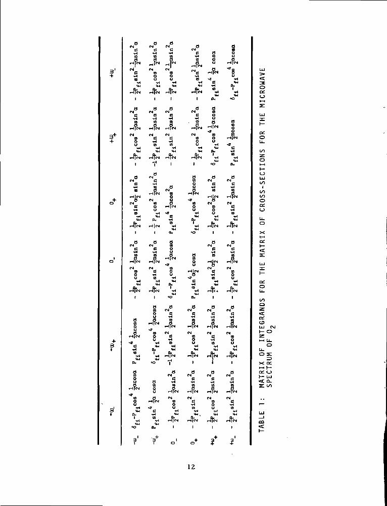
1 Matrix of integrands for the matrix of cross sections
for the microwave spectrum of O 12Li
2 The subroutines of the scattering program and their
functions 20
3 A sample of trajectory output at reference temperature
298°K 22
4 The scattering program input 24
5 Sample input 27
6 The printed output 28
7 The line widths of the pure O microwave spectrum. . 44
8 Selected values for the pure O absorption coefficient^
at 29.8°K about the O, 9+ line (db/km) 45v , f - . • • • - 2
IV
FOREWORD
The work described in this report -was done as part of a research
program on quantitative millimeter wave spectroscopy of atmospheric
oxygen. The project was partially supported by NASA Langley Research
Center under Order No. AAFE, L58-506; and the computer time used
in this research was provided by the National Center for Atmospheric
Research which is sponsored by the National Science Foundation.
During this period of this work the author was employed by
OT/ITS through an agreement with the Cooperative Institute for Research
*)in Environmental Sciences. CIRES also provided indispensible support
for this work.
A cooperative effort of the National Oceanic and Atmospheric Admin-istration and the University of Colorado.
CLASSICAL SCATTERING CALCULATIONS FORDIATOMIC MOLECULES
A General Procedure and Applicationto the Microwave Spectrum of O_
Uri Mingelgrin
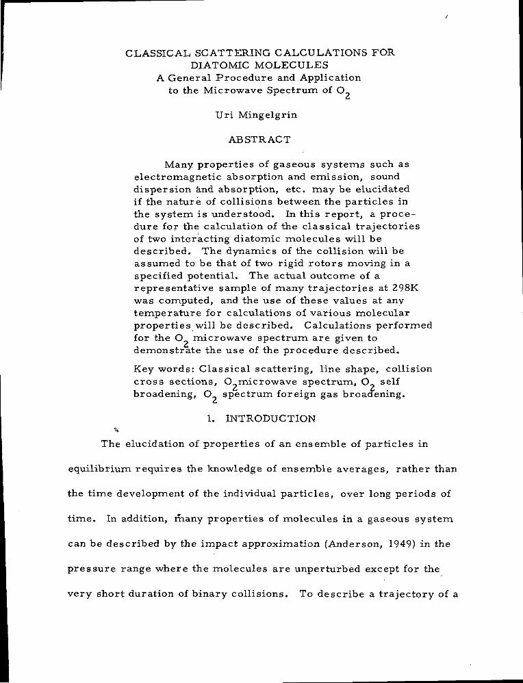
ABSTRACT
Many properties of gaseous systems such aselectromagnetic absorption and emission, sounddispersion and absorption, etc. may be elucidatedif the nature of collisions between the particles inthe system is understood. In this report, a proce-dure for the calculation of the classical trajectoriesof two interacting diatomic molecules will bedescribed. The dynamics of the collision will beassumed to be that of two rigid rotors moving in aspecified potential. The actual outcome of arepresentative sample of many trajectories at 298Kwas computed, and the use of these values at anytemperature for calculations of various molecularproperties will be described. Calculations performedfor the O microwave spectrum are given todemonstrate the use of the procedure described.
Key words: Classical scattering, line shape, collisioncross sections, O microwave spectrum, O_ selfbroadening, O spectrum foreign gas broadening.
C*
1. INTRODUCTION
The elucidation of properties of an ensemble of particles in
equilibrium requires the knowledge of ensemble averages, rather than
the time development of the individual particles, over long periods of
time. In addition, many properties of molecules in a gaseous system
can be described by the impact approximation (Anderson, 1949) in the
pressure range where the molecules are unperturbed except for the
very short duration of binary collisions. To describe a trajectory of a
molecule during such a binary collision, one needs to define the
colliding molecule's initial conditions such as relative velocity,
angular momenta, etc. , and then to solve the equations of motion
assuming some intermolecular potential. One may, therefore, choose
a statistical sample of initial conditions for the various possible colli-
sions and then solve the proper equations of motion. Once a set of
initial and final conditions for a sample of trajectories is given, cross
sections and expectation values for various variables can be derived
which can then be used for calculations of the various relaxation
phenomena and other properties. For example, the microwave
spectrum, the rotational Raman spectrum and sound absorption by OLJ
were computed from the data derived from such a statistical set of
collisions (to be published, also see section 3).
Section 2 of this report will describe how a representative sample
of collisions is calculated, while section 3 will demonstrate the use of
such data in calculation of various properties. A description of a pro-
gram which performed the trajectory calculations is given in section
2. 3.
2. THE CLASSICAL TRAJECTORY CALCULATIONS
The collision between two diatomic molecules was assumed to be
between two rigid rotators moving in a specified potential. This
approximation will hold when:
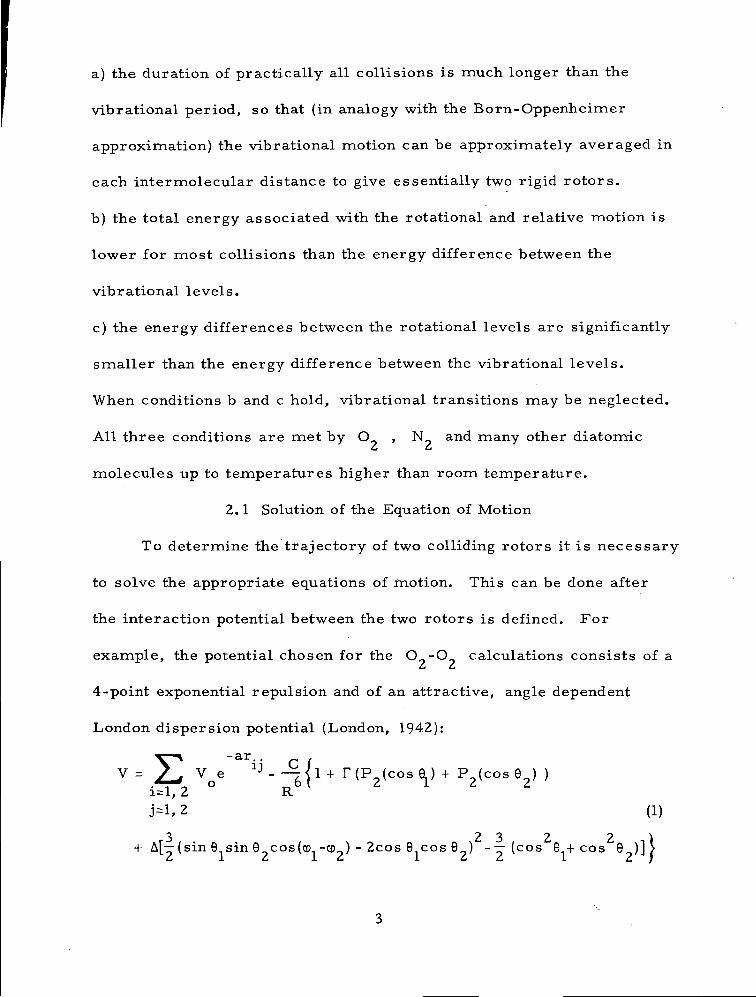
a) the duration of practically all collisions is much longer than the
vibrational period, so that (in analogy with the Born-Oppenheimer
approximation) the vibrational motion can be approximately averaged in
each intermolecular distance to give essentially two rigid rotors.
b) the total energy associated with the rotational and relative motion is
lower for most collisions than the energy difference between the
vibrational levels.
c) the energy differences between the rotational levels are significantly
smaller than the energy difference between the vibrational levels.
When conditions b and c hold, vibrational transitions may be neglected.
All three conditions are met by O , N and many other diatomicLJ £t
molecules up to temperatures higher than room temperature.
2.1 Solution of the Equation of Motion
To determine the trajectory of two colliding rotors it is necessary
to solve the appropriate equations of motion. This can be done after
the interaction potential between the two rotors is defined. For
example, the potential chosen for the O -O calculations consists of aL* LJ
4-point exponential repulsion and of an attractive, angle dependent
London dispersion potential (London, 1942):
Z -ar..VQe 1 J--
i=l, 2 Rj= l ,2 (1)
3 2 3 2 2 )+ A[—(sine sine cos(cp -co ) - 2cos 6 cos 9 ) - — ( c o s 6+ cos 9 )] >
Z 1 Z 1 Z 1 Z Z 1 Z /
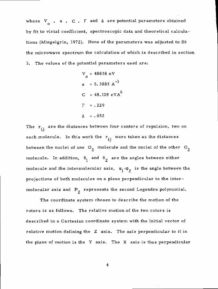
where V , a , C , F and A are potential parameters obtainedo
by fit to virial coefficient, spectroscopic data and theoretical calcula-
tions (Mingelgrin, 1972). None of the parameters was adjusted to fit
the microwave spectrum the calculation of which is described in section
3. The values of the potential parameters used are:
V = 48838 eVo
a = 5. 3883 A"1
C = 48.108 eVA
T = .229
A = .052
The r . are the distances between four centers of repulsion, two onij
each molecule. In this work the r. . were taken as the distancesij
between the nuclei of one O_ molecule and the nuclei of the other OL* £•
molecule. In addition, 0 and 9 are the angles between either
molecule and the intermolecular axis, cp -cp is the angle between the1 £j
projections of both molecules on a plane perpendicular to the inter -
molecular axis and P represents the second Legendre polynomial.L*
The coordinate system chosen to describe the motion of the
rotors is as follows. The relative motion of the two rotors is
described in a Cartesian coordinate system with the initial vector of
relative motion defining the Z axis. The axis perpendicular to it in
the plane of motion is the Y axis. The X axis is thus perpendicular
to the plane of motion. This coordinate system was used and is
described in detail by Karplus et al. (1965). The internal motion of the
rotors is described in spherical polar coordinates. The axes defining
the internal motion are parallel to those defining the relative motion.
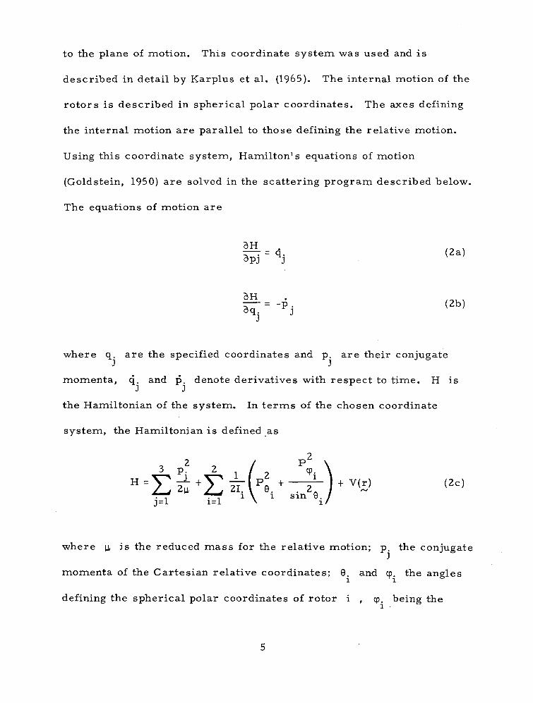
Using this coordinate system, Hamilton's equations of motion
(Goldstein, 1950) are solved in the scattering program described below.
The equations of motion are
*
where q. are the specified coordinates and p. are their conjugate
momenta, q. and p. denote derivatives with respect to time. H
the Hamiltonian of the system. In terms of the chosen coordinate
system, the Hamiltonian is defined as
is
V(r) (2c)
where u is the reduced mass for the relative motion; p. the conjugateJ
momenta of the Cartesian relative coordinates; 9 and cp the anglesi Ti b
defining the spherical polar coordinates of rotor i , cp. being the
azimuthal angle: I. is the moment of inertia of rotor i , and V(r)i ~~>
the potential defined in equation 1. Finally, P , P are the9. CD.i Ti
appropriate conjugate momenta.
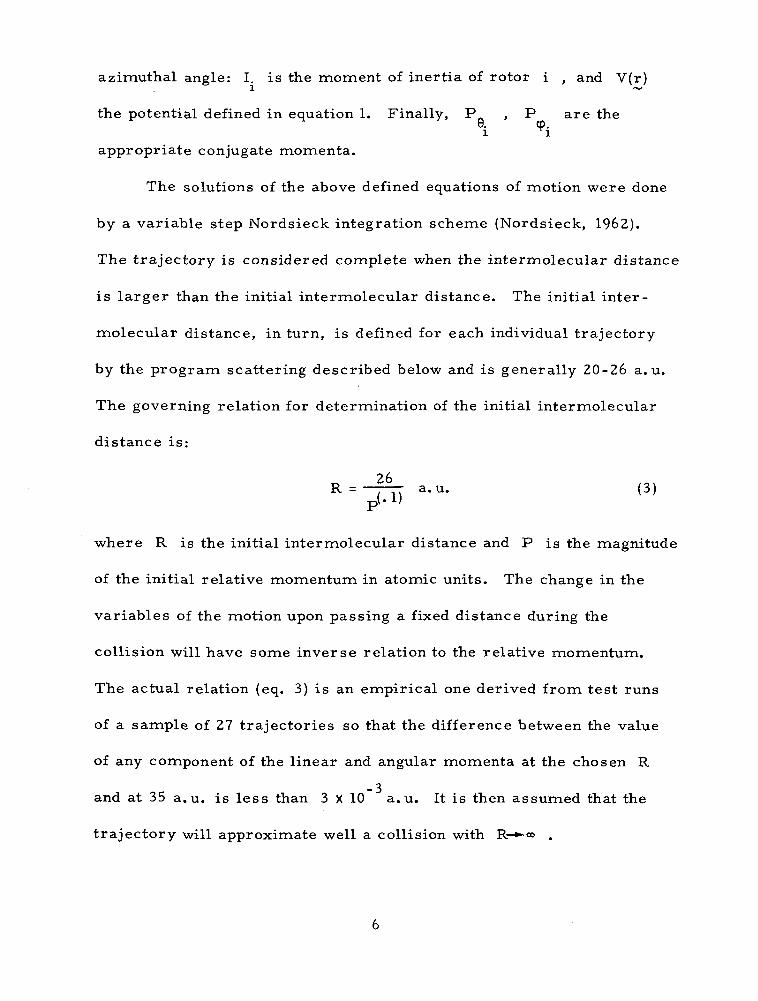
The solutions of the above defined equations of motion were done
by a variable step Nordsieck integration scheme (Nordsieck, 1962).
The trajectory is considered complete when the intermolecular distance
is larger than the initial intermolecular distance. The initial inter -
molecular distance, in turn, is defined for each individual trajectory
by the program scattering described below and is generally 20-26 a. u.
The governing relation for determination of the initial intermolecular
distance is:
R = -pr- a.u. (3)•p\' *•)
where R is the initial intermolecular distance and P is the magnitude
of the initial relative momentum in atomic units. The change in the
variables of the motion upon passing a fixed distance during the
collision will have some inverse relation to the relative momentum.
The actual relation (eq. 3) is an empirical one derived from test runs
of a sample of 27 trajectories so that the difference between the value
of any component of the linear and angular momenta at the chosen R
and at 35 a.u. is less than 3 X 10 a.u. It is then assumed that the
trajectory will approximate well a collision with R-*-« .
As is evident from equation 2c, there is a singularity in the
Hamiltonian at 9. = 0 . This singularity is not of a physical origin
and thus can be removed for a given trajectory simply by changing the
coordinate system. A 180° rotation of all the vectors defining the
initial conditions about the line connecting the centers of mass of both
rotors is performed when the calculations fail because of this apparent
singularity. In this way an equivalent collision which will not pass
through the previously encountered singularity is obtained. The
internal Cartesian coordinates, the components of the angular momenta
of the rotors and the Cartesian relative conjugate momenta are
transformed in a straightforward way. The spherical coordinates and
momenta used in the program are then calculated. The relative
coordinates are not changed by the rotation.
The program in its current version calculates, in addition to the
variables of the motion, the classical rotational phase shifts for both
rotors, defined as the angular change in the position of the rotor in the
rotation plane during a collision (Gordon, 1966). This quantity is not
well defined in non-instantaneous collisions. Before a collision the
rotor rotates in some plane. After the collision is over, the rotor
rotates again in some plane, different in general from the original one.
In an instantaneous collision, the rotor will change its plane of rotation
at a point where the initial and final rotational planes intersect. If no
phase change would have occurred in the collision, the rotor will rotate
up to the instant of collision in the initial angular frequency and follow-
ing that instant in the final angular frequency. At some time t after
such a collision without a phase shift, the position of the rotor in the
rotation plane is well defined. The angle at time t between the above
defined position and the actual position of the rotor is the classical
rotational phase shift. If the collision is not instantaneous, and during
the collision both points of intersection of the initial and final planes of
rotation are passed one or more times, the classical phase shift is not
well defined. The procedure adapted for defining the classical phase
shift is as follows. The time of closest approach in a collision is
determined. Then, the two apparent phase shifts were calculated by
assuming the rotor changed planes of rotation at both times of inter-
section of the initial and final rotational planes nearest to the time of
closest approach. These two apparent phase shifts are designated as
v and v . The difference between the two points of intersection ofJ. L*
the initial and rotational plane is, of course, TT radians. If we call the
angles between the position of the rotor, if it had rotated up to the time
of closest approach in the initial angular frequency and the points of
intersection of the initial and final rotational planes, 3 and (3 , then
the weighted average values of the various functions of the phase shift
(F(v) ) are given by
F(v) = Ffv^l— I + F(v2)l — /
2. 2. Statistical Sampling and the Effect of Temperature
To obtain a representative sample of trajectories, a procedure
formulated by Conroy was used (Conroy, 1967); a Conroy case II for
non-periodic variables with his parameters for 12 variables and 1861
points was utilized. Conroy's procedure for multivariable sampling
selects sampling points so that each variable is sampled uniformly
along its range. For periodic variables one period is sampled. For
non-periodic variables a transformation must be applied to let the range
of the variable be 0 to 1 . For every variable a parameter k , whichXI
is the ratio between some odd integer smaller than the sample size and
the number of points is defined. The sample size is chosen to be some
large prime number. The values of a variable (x.) sampled may beJ
selected by a number of schemes. In the case of "Conroy case II" the
values selected are:
x. = j- k - e. j = 1,2, . . . , -e (4)J x J
where 4 is the sample size and e. is an integer chosen so that x.
falls between -1, 1 . The absolute value of x. is then taken. Conroy
demonstrated that one set of points selected by such a procedure will
optimize the sampling. The actual parameters k chosen wereX.
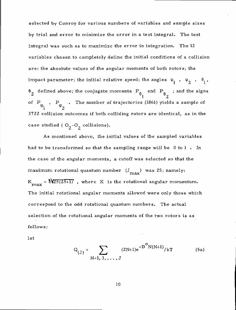
selected by Conroy for various numbers of variables and sample sizes
by trial and error to minimize the error in a test integral. The test
integral was such as to maximize the error in integration. The 12
variables chosen to completely define the initial conditions of a collision
are: the absolute values of the angular momenta of both rotors; the
impact parameter; the initial relative speed; the angles cp , cp , 9 ,i. C* J.
9 defined above; the conjugate momenta P and P ; and the signs2 91 92
of P , P . The number of trajectories (1861) yields a sample of
3722 collision outcomes if both colliding rotors are identical, as in the
case studied ( O -O collisions).L* £*
As mentioned above, the initial values of the sampled variables
had to be transformed so that the sampling range will be 0 to 1 . In
the case of the angular momenta, a cutoff was selected so that the
maximum rotational quantum number (J ) was 25; namely:^ max '
K = nV25(25+l)' . where K is the rotational angular momentum.max °
The initial rotational angular momenta allowed were only those which
correspond to the odd rotational quantum numbers. The actual
selection of the rotational angular momenta of the two rotors is as
follows:
let
N=l, 3,. .. , J
10
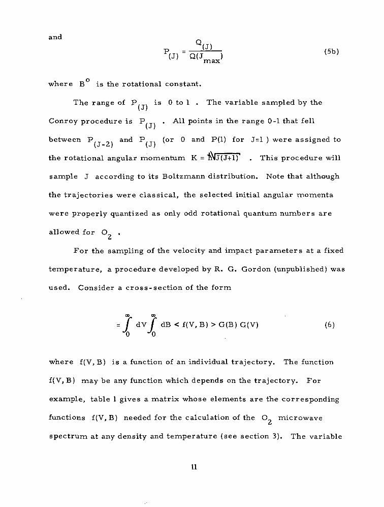
and
P(J)max
where B is the rotational constant.
The range of P , T > is 0 to 1 . The variable sampled by the(J )
Conroy procedure is P. . . All points in the range 0-1 that fell
between P and P,T. (or 0 and P(l) for J=l ) were assigned to(J -Z) ( J )
the rotational angular momentum K = rNJ(J+l) . This procedure will
sample J according to its Boltzmann distribution. Note that although
the trajectories were classical, the selected initial angular momenta
were properly quantized as only odd rotational quantum numbers are
allowed for O .Li
For the sampling of the velocity and impact parameters at a fixed
temperature, a procedure developed by R. G. Gordon (unpublished) was
used. Consider a cross-section of the form
00 CO
= f dV f dB < f(V, B) > G(B) G(V) (6)C\ f\
where f(V, B) is a function of an individual trajectory. The function
f(V, B) may be any function which depends on the trajectory. For
example, table 1 gives a matrix whose elements are the corresponding
functions f(V, B) needed for the calculation of the O microwave
spectrum at any density and temperature (see section 3). The variable
11
3'+
3+
0+
1O
.
3l
3'i
8CM
B•HCO
r-lpM
CMB•rlto•rtIM
1
CM°B•HCO
rH)|CM
CM01ou•rlIM
r-ftcM
1
8CM
Bi-l09
CMB•HCO•rlIM
rHtcM
«
8CM
B•rlCO
iH[CM
CMCOOu•HIM
i-lfcM
1
8
IfHffM
B•HCO•rl
PH
801Oo
|H|CM
CO0u•HIM
PL.11-1CM
I
3
aCM
B
01
CMtoOu
•HIM
1
^8B•Hto
CMB•rl01•HIM
r-f|cM
V
aCM
B•Hm
i-l|CM
CMtoOu•HIM
PH
r-t|(SI
1
aCM
B•rlCO
r-lJcM
CMB•Hm•rlIM
i-ffcMJ
1
801o
rH|CM
-a-aou1-1IM
PH1•H
•o1"
8toou
r-l|CM
Bi-l01•HIM
PH,
'3
8CM
B•H
^CM
COo0ftIM
rHt<M
1
CM°B•HCO
•HJCM
CMB•rl01
•HIM
rtfcM
1
8CM
ao
JL^j
B•HCOi-l
a.
8COou
r-lfcM
COou•HIM
•H
*o
8CM
B•HCO
i-ifeM
CMB^4to•HIM
-flcM
r8
CMB•rl
JLCM
COou•HIM
rtfcM
1
1O
8CM
Bi-lto
CMe
a-rlIM
1
CM8
Bi-l
. CD
rH|CM
CMtoOUi-lIM
i-lTcM
1
8toOu
r-IICM
COOU•rlIM
PH1•H
<O
8COou
vHlcMJJ
-aB•Hto•rl
tt.
8CM
B•H
§iHfCM
CMtoO0•rlIM
r-lJcM
1
aCM
B•H01
rH|CM
CM
•H01•HIM
r-<|CM
1
o+
801ou
r^ffM
-3B
CO•H
PH
§
OUa
rH|CM
COOu•rlIM
PH1•rlIM
«O
8CM
B•HCO
CMCOou
•HIM
rntcM
«
8CM
B•rlCO
"ITCM
B•Hto•rlIM
rH|c<
1
8CM
B•H
r-lfcM
CMB•rlco•rlIM
1
8CM
B•rl
?iH|CM
CMaou•HIM
rnfcM
1
I
aou
>H|CM
"8u
•HIM
i-tIM
«O
8COou
iHfCM
-a-B•rlCO1-1IM
8CM
B•H
?rH|CM
CMB•HCO•rlIM
rHJCM
1
8CM
B•rl
•-IJCM
CM01Ou•HIM
1
8CM
B•H
1r-lTcM
CM0ou•rlIM
rnJcM
1
8CM
B•H
JM
CMB•rl01i-lIM
r#CM
1
|
1
UJ
<c2Oce.tj\r-l
^
UJ~T"
h—
o:o\t
^f)zor-l
O1 1 1
LO1
oooo0o;o
u.0
X
Q£(—
S.
UJ-l-> ^r—
/-^Ou_
ooa
^^0UJ OO1- 0
i_i i »0
u.o 2:
x o:
C£. 0i 111r LJJ^ Q-'SL to
• •
LU
CO
^
12
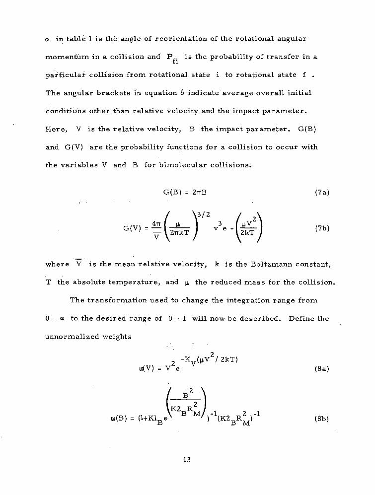
a in table 1 is the angle of reorientation of the rotational angular
momentum in a collision and P is the probability of transfer in a
particular collision from rotational state i to rotational state f .
The angular brackets in equation 6 indicate average overall initial
conditions other than relative velocity and the impact parameter.
Here, V is the relative velocity, B the impact parameter. G(B)
and G(V) are the probability functions for a collision to occur with
the variables V and B for bimolecular collisions.
G(B) = 2-nB (7a)
(7b)
where V is the mean relative velocity, k is the Boltzmann constant,
T the absolute temperature, and p, the reduced mass for the collision.
The transformation used to change the integration range from
0 - oo to the desired range of 0 - 1 will now be described. Define the
unnormalized weights
2 -K (uV 2 /2kT)(B(V) - V e (8a)
(8b)
13
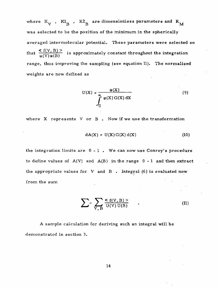
where K , Kl , K2 are dimensionless parameters and RV B B M
was selected to be the position of the minimum in the spherically
averaged intermolecular potential. These parameters were selected so
that — ' . is approximately constant throughout the integration
range, thus improving the sampling (see equation 11). The normalized
weights are now defined as
U(X) = =^ (9)r ou(x)G(X)dx
•'O
where X represents V or B . Now if we use the transformation
dA(X) = U(X)G(X)d(X) (10)
the integration limits are 0 - 1 . We can now use Conroy's procedure
to define values of A(V) and A(B) in the range 0-1 and then extract
the appropriate values for V and B . Integral (6) is evaluated now
from the sum
< f ( V , B ) >
A sample calculation for deriving such an integral will be
demonstrated in section 3.
14
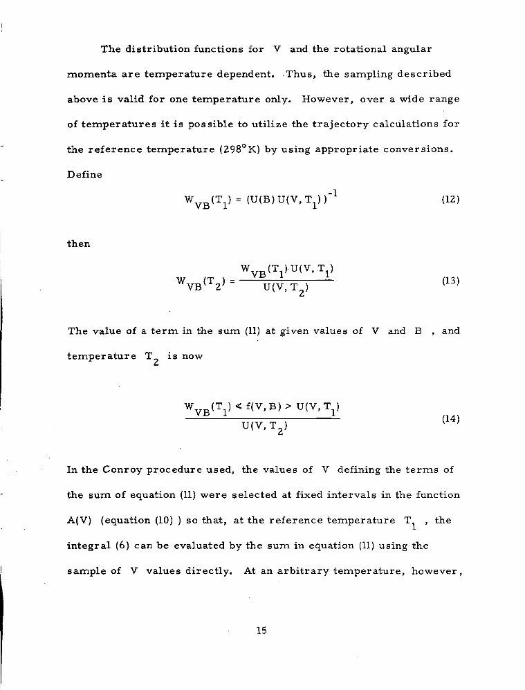
The distribution functions for V and the rotational angular
momenta are temperature dependent. Thus, the sampling described
above is valid for one temperature only. However, over a wide range
of temperatures it is possible to utilize the trajectory calculations for
the reference temperature (298°K) by using appropriate conversions.
Define
) = (U(B) U(V, T) )"1 (12)
then
W (T )-U(V,T )W (T ) = ———= —
VB 2 U(V, T )2
The value of a term in the sum (11) at given values of V and B , and
temperature T is now
W (T ) < f ( V , B ) > U ( V , T )VB l L
U(V,T )
In the Conroy procedure used, the values of V defining the terms of
the sum of equation (11) were selected at fixed intervals in the function
A(V) (equation (10) ) so that, at the reference temperature T , the
integral (6) can be evaluated by the sum in equation (11) using the
sample of V values directly. At an arbitrary temperature, however,
15
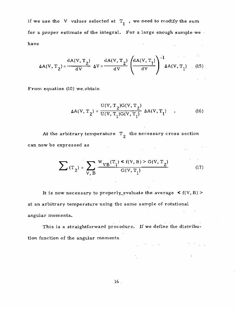
if we use the V values selected at T , we need to modify the sum
for a proper estimate of the integral. For a large enough sample we
have
dA(V,T ) dA(V,T ) /dA(V,T
dV dV
From equation (10) we.obtain
U(V,T )G(V,T )
At the arbitrary temperature T the necessary cross sectionL*
can now be expressed as
W (T ) < f ( V , B ) > G ( V , T )
It is now necessary to properly^evaluate the average < f(V, B) >
at an arbitrary temperature using the same sample of rotational
angular momenta.
This is a straightforward procedure. If we define the distribu-
tion function of the angular momenta
16
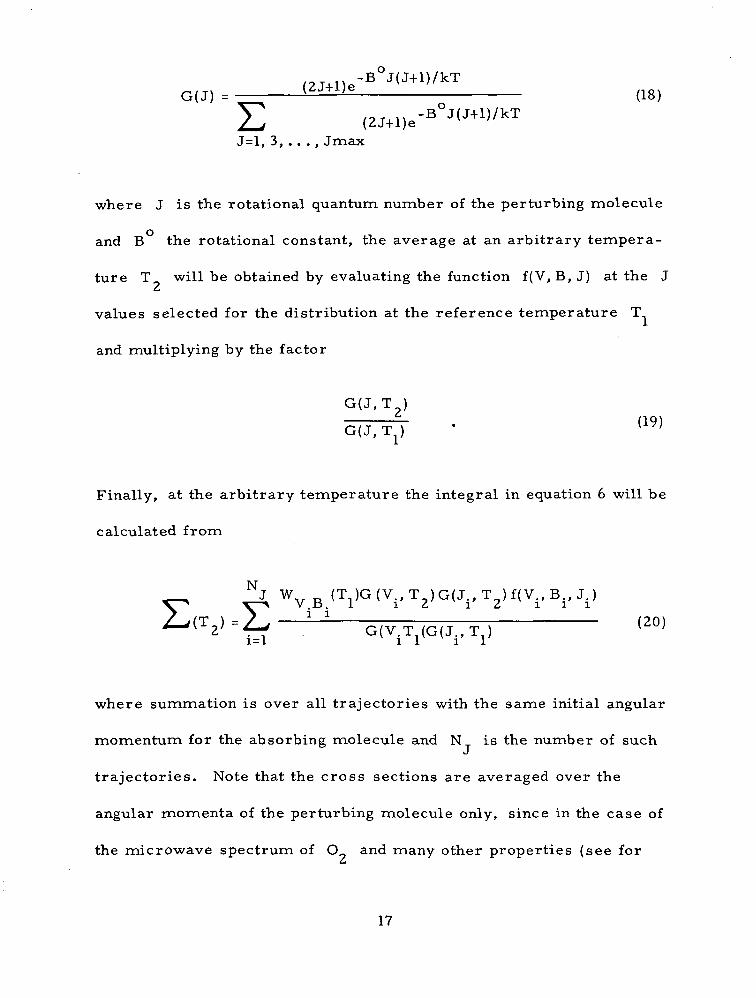
G(J) = v ; (18)
J=l, 3, . . . , Jmax
where J is the rotational quantum number of the perturbing molecule
and B the rotational constant, the average at an arbitrary tempera-
ture T will be obtained by evaluating the function f(V, B, J) at the J
values selected for the distribution at the reference temperature T
and multiplying by the factor
G(J ,T 2 )
Finally, at the arbitrary temperature the integral in equation 6 will be
calculated from
G(V , T )G(J . ,T ) f ( V ,B J )1 L* 1 LJ 111
G(V T (G(J , T )(20)
where summation is over all trajectories with the same initial angular
momentum for the absorbing molecule and N is the number of suchJ
trajectories. Note that the cross sections are averaged over the
angular momenta of the perturbing molecule only, since in the case of
the microwave spectrum of O and many other properties (see forLJ
17
example section 3), these are the necessary averages. Averages for
both molecules' angular momenta can be treated similarly, simply by
summing overall values of the rotational angular momenta of both
molecules using the proper Boltzmann factors. For example, equation
(20) will have to be multiplied by the factor
where J. indicate the rotational quantum number of the radiator and
the sum will be over all trajectories.
2. 3. Description of Program and Output
The 4-body trajectory calculations described above are executed
by a classical scattering program fashioned after a reactive scattering
program written by K. Morokuma and L. Pedersen. The present
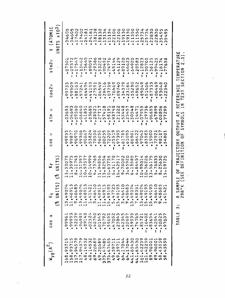
A list of the program described below as well as the output for a
complete set of trajectories at 298°K can be obtained on request from
the ITS MM Wave Transmission Spectroscopy Section. (See Table 3 for
sample output and text for output description.
18
program is written by the author for the CDC 6600 and 7600 computers.
An average trajectory calculation takes 4 seconds on the CDC 6600.
Reference will be made to the actual variables and subroutines' names
to simplify the understanding of the program listing for those inter-
ested in obtaining it.
The following items will be described:
a. A list of subroutines and their functions is given in table 2.
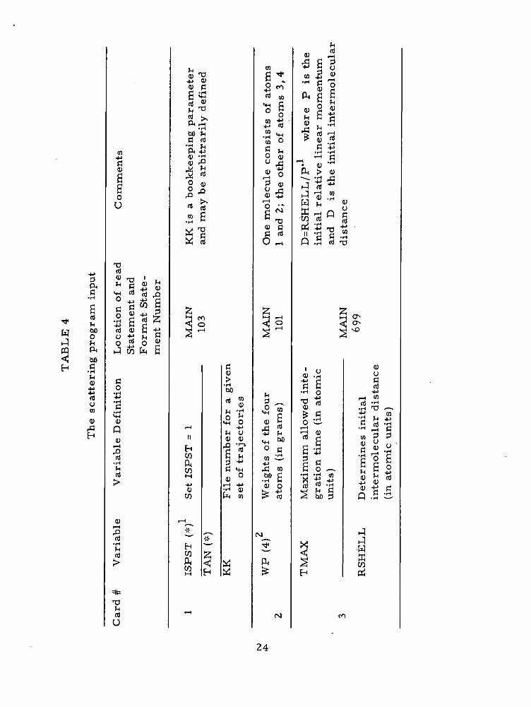
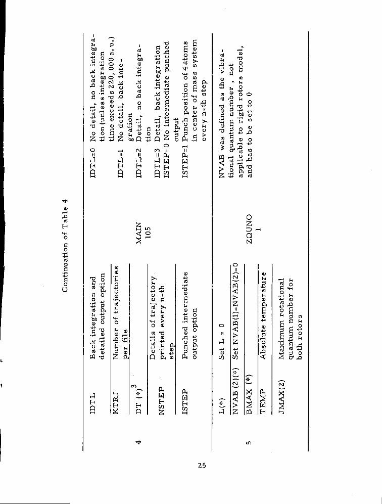
b. The input to the program. A list of the input appears in table 4.
The subprogram and statement numbers of the format statements
according to which the input variables are read also appear in
table 4. A sample input appears in figure 5.
c. A description of the way the program executes a trajectory
calculation.
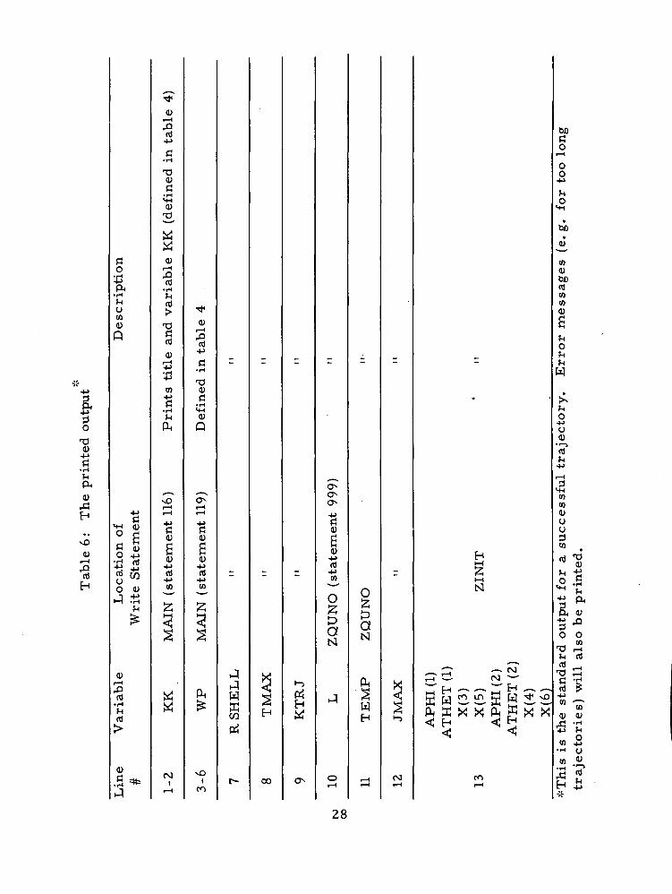
d. The program output. A sample of the punch output is given in
table 3. A list of the printed output parameters is given in
table 6.
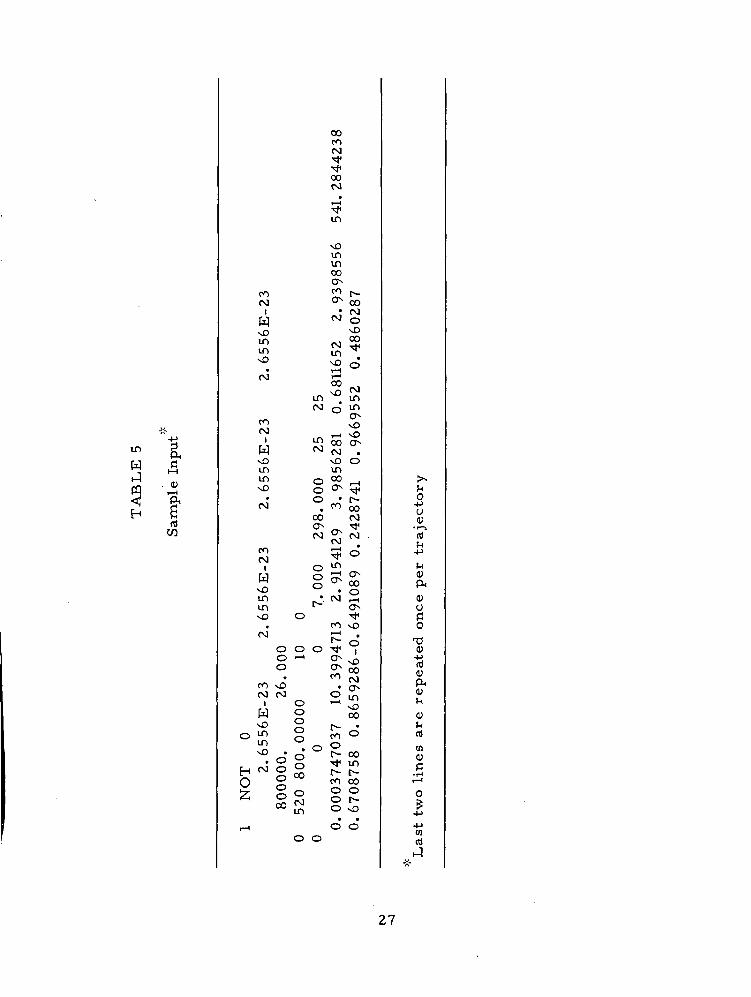
The program input consists of a set of 5 cards per set of
trajectories followed by two cards per trajectory. A sample of the
input is given in table 5. The input variables, definitions, and the
location and statement number of the associated format statements are
listed in table 4. The input includes some options regarding the form
of output, the conditions for the set of trajectories and data which
19
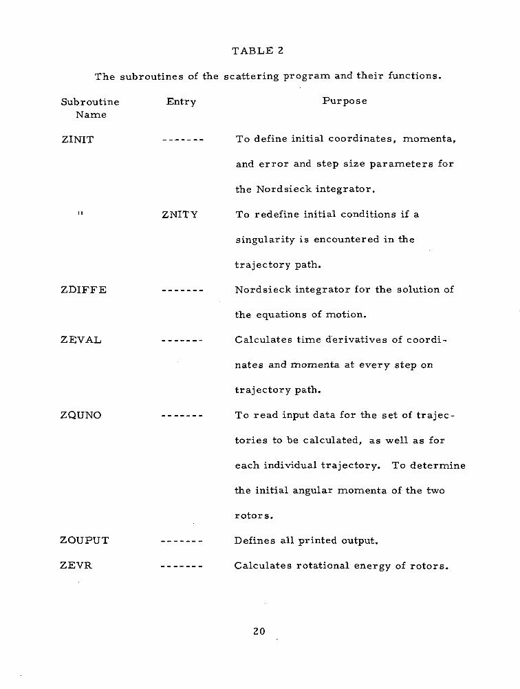
TABLE 2
The subroutines of the scattering program and their functions.
SubroutineName
ZINIT
Entry
ZDIFFE
ZEVAL
ZQUNO
ZOUPUT
ZEVR
ZNITY
Purpose
To define initial coordinates, momenta,
and error and step size parameters for
the Nordsieck integrator.
To redefine initial conditions if a
singularity is encountered in the
trajectory path.
Nordsieck integrator for the solution of
the equations of motion.
Calculates time derivatives of coordi-
nates and momenta at every step on
trajectory path.
To read input data for the set of trajec-
tories to be calculated, as well as for
each individual trajectory. To determine
the initial angular momenta of the two
rotors.
Defines all printed output.
Calculates rotational energy of rotors.
20
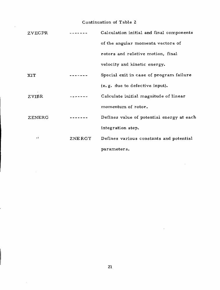
Continuation of Table 2
ZVECPR
XIT
ZVIBR
ZENERG
ZNERGY
Calculation initial and final components
of the angular momenta vectors of
rotors and relative motion, final
velocity and kinetic energy.
Special exit in case of program failure
(e. g. due to defective input).
Calculate initial magnitude of linear
momentum of rotor.
Defines value of potential energy at each
integration step.
Defines various constants and potential
parameters.
21
<_5 COi—i O
O XI—eC CO
00
CMCOao
COoo
COI—I—IZ
COoo
CO
I I I I I
I I I I I I I I I
o~» f- o >JD t~- -J >o co in o** o en ir> m i-< t\i oj <o o •—< i*-
Cr^ co O^ c^ ^O oc tr^ C5 fvj fNj if\ to f^^ ^3 ij v^ c^ LO if\ o^ ^HO^ O^ vO O^ C^ C i CO *O ^5 f J lA ^~ " *~^ *>O ^O ^~~ C l O^ ONJ CO
I I I I
o o o j o o m i o
CO•
00
UJ Za- o
UJ CO
Z I—LU X
o: i— i
I— co
oCD
a. >•I— co
o u.o
o oi— >-"CJ I—
o: LL.I— LU
QLl_O UJ
LLJLU CO
Q-S <0CO CO
enet OJ
CO
22
determine the initial conditions of individual trajectories. The condi-
tions fixed for the set of trajectories are: The weights of the four
atoms, the maximum integration time allowed per trajectory, a
parameter defining the initial intermolecular distance, the number of
trajectories per set, the temperature and the highest rotational
quantum number allowed. The variables defining the initial conditions
of a trajectory were listed in the text (section 2 .2) and the actual input
data per trajectory are given in input cards 6 and 7 as listed and
defined in table 4.
The basic features of the actual execution of a set of trajectory
calculations will now be described. First, the necessary input for a set
of trajectories is read. Next the various reduced masses (array W) are
defined from the masses of the four atoms (array WP) in the main
program. Subroutine ZINIT is then called. ZINIT calls in turn sub-
routine ZQUNO where the array XU(N,II) is defined. This is the array
of the functions P(J) defined in equation (5b) for both rotors. The
determination of individual trajectories starts at this point. ZINIT is
called again. It in turn calls ZQUNO where the input data for the
individual trajectories are read and the quantum numbers J(array JAB)
of the rotational angular momenta for both rotors are determined. Upon
returning to ZINIT the input data are used to define the initial coordi-
nates and conjugate momenta (the arrays QI -- the array of the
23
"5Ac•iH
a^ 2W o°r^l h
PQ f1"
H g"rH)_|0
"ftloCO
0
CO
"c0aao
U
n)0 — * i^D l_i^ (~* 0
^ rt Id rQ0 •!-> *" P
0 <U -4-> ,5.2 g ni S-M C rlrt 0 C -eO -r» tl H
0 «| 0 «J 55 fa S
Vari
ab
le D
efi
nit
ion
3n)•H
rt>
=*:
cdU
^_> 00 fia ^2 - Srt >>DO 'JH
•S rt
PU -Meu -H<1J rQ
"iy rtO cp
rQ
m rt*.2 a>y< ^
W cd
M CO<J 0
rH
I I
H
COM
•4-"V
CO
rH
E-iCO
CO1— 1
-X-•
£H
H
C0
Fil
e n
um
ber
for
a g
i\se
t o
f tr
aje
cto
rie
s
M
rH
enC ^
•S ^cd w
o oCO -HCO ^
o 0c ^,O a;
U ^fl) "*"*
" r G0 '[ *
i-H
a ^0 dfi rd0 rH
IsS "
Weig
hts
o
f th
e fo
ur
ato
ms
(in g
ram
s)
00
2J,
£
00
0 rH
£ £ 2S °w -S ®>H C o0 g
(U ° 0M £ "r*<u .5f2* rt '
e '*•H -|H
*"• 0 'H
PH > 0-~^ -H r!
T ** *>i— 1 njr-1 fl) *_J
E S
•w 3 |^ '^ "c ^P -S rt ^
^S^
t
0 -H
Max
imu
m a
llo
wed
in
tg
rati
on t
ime (i
n a
tom
un
its
)
^**I
H
0o
Dete
rmin
es
init
ial
inte
rmo
lecu
lar
dis
tar
(in a
tom
ic u
nit
s)
T
•H
COPH
CO
24
^Fcu
^^•sHmOflO
•H•4-1mSs
•43floU
U i ii 91IP.I I P !:y & o o - H ri JH <u o co™ « ro « ^ e - t J ,* ri ft•° -g N -g y -S .2 g g u§ ' S ^ ^ 5 * "g 5 ^ »c M ;R " 2 -H o rf* w u - ° rtS w ° £— _| (i) \U ,_) ft A " — . . -#-»
^ ^ 0 - ^ C ^JH g. g '-2 S * -2 c • - 5 ^ ^ •§ fiU - E ^ a j O ^ ^ C d ^ ? , > >
T 3 r t < U T 3 4 j n i _ n J - ' - | Q j y < u hfir|rt-*->P!-tJo-&SuS
O rt t" rt fll /^ fll O r^ Lw > - ) O t j < u o ( w . _ i H p _ , ^S -ji £ fc bo P -^ p Z o PH .S «
O ,_!O ^H CM ro II II
II II II II pL, PHJ J .J] J M WH H LH H H HP P P p co co1— 1 1— 1 1— 1 h-H I— 1 1— 1
§ s< 2s
•s §C •!-<rt ftfl 00
•43 ?rt ft
Bac
k i
nte
gr
deta
iled
ou
tID
TL
COcu
•HfHO
•4->y
0)••— 1n)M
J ^
Nu
mb
er o
f 1
per
fi
leK
TR
J
fV^r1 1
5THp
^
>•*hO rfl
•4-> +>O 1CU fl
•*? .co ;><Li !-,
Deta
ils
of
t:p
rin
ted e
ve:
step
NS
TE
P
cu•*->ni-HT)
CUgfH^fcu fl
Pu
nch
ed in
t
ou
tpu
t o
pti
o
IST
EP
*i •— i
* 1-a -•-> 2•> a gfl) Ws - ^* h 0w <" o o*! h 0rQ C T-J 4J0) g -H ^
S fl W> CD^ S 'S ro
(U H aiV B 3 5S S ® o> ^ 5^ c^'rt raw _»
CQ r-< U 2
^ | a^> .0 ft flS 4-> rt rt
o1-7z^> ^aN
on
-ncu
CO
^r^
0I I
00
CQ<I I
I Se
t N
VA
B(i
;
•&
OvT
NV
AB
(
?r
5
BM
AX
cu»H
5•JJctfhcuftS
Ab
solu
te t
eiT
EM
P
•-J Vn2 0fi m*.2 h•e <u45 -0
o S
Max
imu
m r
qu
antu
m n
ui
bo
th ro
tors
oo"
32i-n
25
•
coi— t&
CO
H<+HO
co•i-t.4_>cogR
•H•g
OU
f-<CO
•~t ^ M
8-1: s.i— i •(-* ...
s g s s• H H
•!-> S^1 rrt 0 O
co ^ ri ^•Sc 13P< -H 4J COM « -a ft2 ^ •* £
,£ _ <U ^•4_> CO ?> .+J
,, cd ^ X t^^ ni CO rrth co co .£ *5rt +j .5 * ^
.E 'H 'O -*->T) T) <° CO Oc S « c -g «rt § ^ 3 s ?a o ^ T3 o 43
OZD OJaN
>s
Initia
l re
lative
velo
cit
(in
ato
mic
units)
>
Impact
para
mete
r (in
ato
mic
units)
n.+-H5!I H1— 1
«
£
1
O
coboaCO^
oo9-
i-H9
oo"
HH
ffiOn<J
ti0
CObofiCOVi
00CD
•i
t— 1CD
00
HHEEH<
oo<!a
•H
""«>
H
pq>
vO
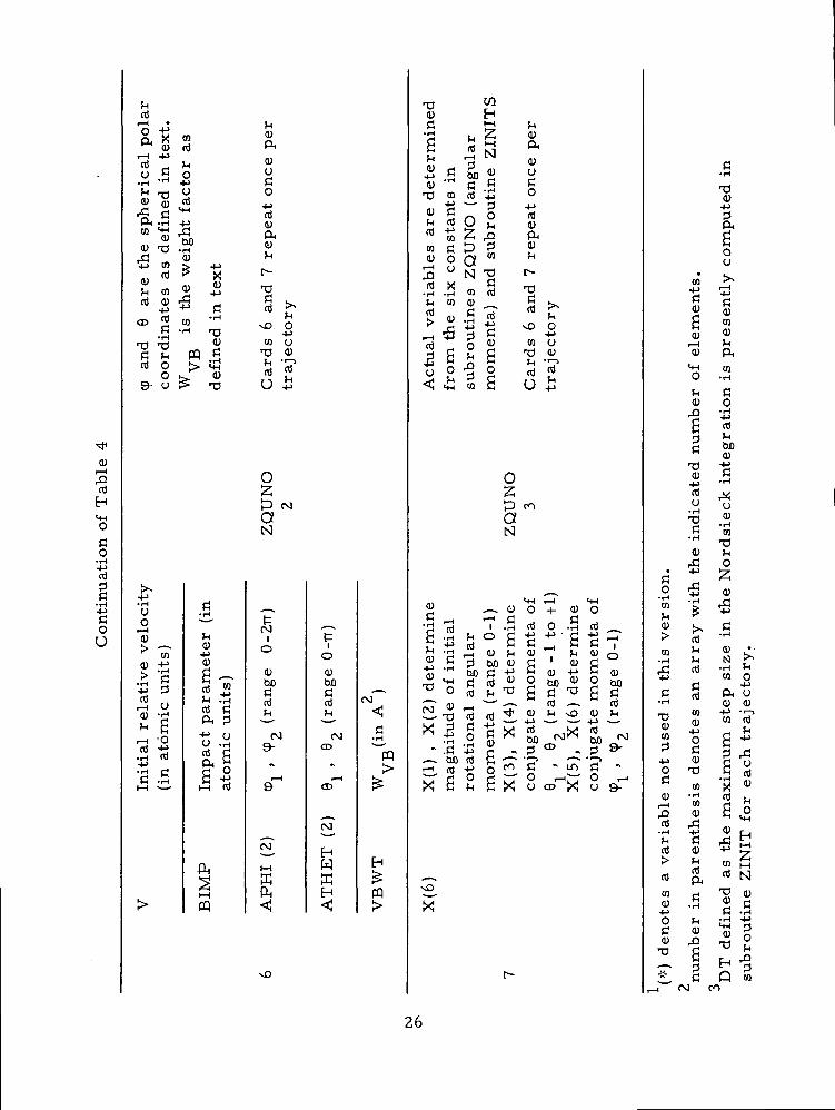
-o ^co Hfl "-< h•S ^ S coa co - ftS "3 «* fi §> 2 y4, "-i c fi fj
fH ^^ -^
T3 co nj 4J O** ' — ' d -(->
£ S n o 13
- ^ § ^ S,03 c ^ S £co o O ^_ i . . X^-
3 ° N -0 t-CO X fi rr-l.2 .5 w co "2^H CO CO _ 5 t>>co m « "^ rt rp> J2 -^ | o o-i ^ d « m tlnj 5 co co o1 a | a -g .2,0 0 •£ 0 rt CO< & s a o i
ozP OO
aN
/it m i— i m5J — , co o + co o" .—1 r~l (H C
•Jj rrt 1 .H Cti O .H (0a -3 s ° a ^ ^ • a 3 ?1 3 -3 & £ g . ss o; H b D c J - < - > ^ - i c o - * - > ' - i ( i )
•S -o g 2 -S | ff 5 g ff•••i ^—^ " «* " *rlTV d) i - — • ™ "^" ™
Ci-O rt rtS^i-S^^X d d - ^ ' x ' r t b*1 13- .2 S * 3> M N•> .rt -j3 S . d " 3 3 - d ^ -. — . OD CO C ^~- "~> • — • """- H f t f - i - i o 0 0 ^ - " ^ f i "r^ £ o c rT o i-i|~r o ^X C h H X o c D X c j g -
-.sO
X
r-
G•i-l
T3(U_j_idftaoCJ
• •>.to ^•g q32 Ss sa; co
•— i ^<CO PH
t-l COO -r-l
>H CCO OA ._J
-2 +3a 22 &d bo
fliu^rrt -t-
1
« ci > *rH
§ «• rH -.
^ .Sf-4 "c to-rt 13co h
rC 0
C ^ ^0 -5 CD
ible
not
use
d i
n t
his
ve
rsi
lesis
d
en
ote
s an a
rra
y w
ii
maxim
um
ste
p siz
e in
thi
for
ea
ch t
raje
cto
ry.
lu ' ni• H 4J CO r.t (~! rH L1
" R AH t_im co -t-1 t!> jj co aoi g, «« Nw m ^5 <o
1 f I-SC CO ^1 ^" Qj /^
4J 3 -S 28 H ^• — - d ^ s
^L B P S^ oo en
26
-X-•£- a
w £^ «>M -JS< ftH S
rtCO
ro00
1
WNO
mmNO
•00
ro00
WNO
mmNO
*
00
ro00|
WNO
inmNO
.
00
o0o
ro NO00 00
1
NO
T
02
.65
56
E8
00
00
0.
! 1
COCO00•<t^too00
'in
NO
ininCOON
CO [N_
<^ 00• oo
00 0
NO
00 2m ^NO 0-r-Hl-H
^ Nm ^ S00 0 ID
ON\J^0
^ ^H xOLO rn HN_ _ ***J W ^N 00 .
NO O
in0 °° _<<=> ^ ^o • r-. ^ oo
00 00ON •<*CVJ ^00
3 oTT *•*o »£] _§ ££0 . 0
• 00 ,-(r- o0 -NH
CO NO
£ •^- o00^ ,1-1 t> NO
^». ^**o ooco ^\1 ' 00. ON
o ino -i !
52
0 8
00
.00
00
0, 0
00
37
47
03
7,6
70
87
58
0. 8
1
• •
o oo o
>-
•aje
cto
r
H•(->
J-l0)ftr**
cuuno
T)IP
*>n)a;ft<Dk
(U
nJCO(UC
•Hi— I
0£•!->
4->CO
nJJ
-X-
27
H->1rH,
O
T!CU
-4->c•iH
rH
ft
cuAH
xO
cui— t•8H
C!o•i-t.4^ft
•HrHUCO(UP
Lo
cati
on
of
Wri
te
Sta
tem
ent
Vari
ab
le
cu.s*HH
^cu
i-H
•8•4-J
fi•rH
T3CU53£0)
T3
MMcui — if\
"aIU•rHrH(D
>
T3Cni0)
i££
COH->c•rH
rH
C^
.O>*^i-H
MA
IN (
state
men
t 1
XM
PO1
I— 1
•*cu
I— t
•8•4-*
•iH
T3(UC«cuP
Q\i-H
MA
IN (
state
men
t 1
OH£
vOi
CO
_
-
R S
HE
LL
r-
—
-
TM
AX
CO
_
r
KT
RJ
o
^
c>o0s
ZQ
UN
O (
state
men
t
•-3
o
^Z
QU
NO
TE
MP
r-H_- [
„
-
JMA
X
00
_
• i
H
i— tN
*— **
^^ ^ -LI HH •i— *^ *•"•• ^^ f *«^ ** ••• *«
ffi W 2-^S W ^>o^ g x x ^ g x x
^ ^
CO,_^
w>JH
or-H
O
OH-"
oMH
•bo
»
cu
CO0)CUDrtCOCO0)ar-lOrHt .MwrA
JHO
4->UCUr~Jfl)
ft4J
[3COCO<UUU3CO
-•gIH +»
-21R °-Qi cu^ r DO O_ CO
T3 r-<IH OJnJ
rr! --1TJ I-Hs -d2 £n • — •
CO
<L> CUrj -H
"2 rH
CO 5•H y
CO «"-< 'Z?H R)
M h^ •(->
28
d0
•rt-4-Jrt3c
•rt•4->JH
0USO
cui-H
•SH
Desc
rip
tio
n
-y*S cu
s iO 4->• r-t /H
rt|u UJ
o cuJ *"1— t .rt
MK^
^
Vari
ab
le
cu.S*A
cuuCrt•»->CO
•rt'O
Lec
ula
ri iogHcu
•*->C
• rt
i — 1rt
•rt•»->•rtC
•rt
CU
•4->
mOcut-trt
&CO
I ICMwrt
NWrt
•*i— i
cu}-i
2-§^ m? 0
•5 oSo-Ll J^M r-**
ft u. . cu
rdsi
ec
kN
ord
si
^1*4-»
^ ,
5 Smd. ,.
ax
imu
m s
tep si
ze i
= e
rro
r p
ara
mete
:
S -j
S11 rtH rtP W
ooCO
-(->acu£curt•CO
"Hi— i>7nSI
DT
ER
RO
R
-)->Kcu-t->
•VSrt
= d
efi
ned
in t
able
4
i iH£EP>
VB
WT
^>cuCO
cuJ2+3fi
•H
>sMO
-l->Ucu•i— irtfn
-4->
cu5
fin
ed i
n t
ab
le 4
qu
en
tial
nu
mb
er
oi
cu cuT3 co
ll uV Ojf [ \J
ty* ^r
M 0M £
mt— i
i — irt
•iH4-1
;a«8<u g*J<« eo cuc
CO fi
•s g,cu Cc .l-\ l-l
Mrti — i&flrt
, — i
tati
on
a
0M
i-Hrt
•rt4->-rt
• rt
- x
, y
an
d z
co
mp
cro
tati
on
al
an
gu
laro
tor
1 ( ft
un
its
):
mag
nit
ud
e o
f th
e
i— ii— iZ<
CO
c\r•«i— inH- 1
i — I•t
1— 1
z<
I I
I — 1
U3z<
Hi— iPn1-Mp0N
i-H
t/>
§
-co-M•H
3
*c1— 1h0
mo
men
tum
of
rot
roto
r 1
<+•!O>s00itcuC
init
ial
rota
tio
nal
en
i-H
H<
i-H
5
1— 1
J .HO
^ _*
oVH
MHOl_.
nu
mb
e]
Sr-<3IT&
(ato
mic
un
its)
: in
itia
l ro
tati
on
al
ni-H
CQ<T
l-l
i-H
PQ<i^
nivvCOC
,c!•4-"
O-t->
CD
.S-ocoftCO<U
S-0 h0 O
-MCM O
M *0 JH
+? 0O MH
^ «h --1
£ £
CO -rt
0) ^•-H r>•s -5.2 -0t-< curt S> IT!r MH(U <"^ -0H
Hh- 1Prt1-MPoSI
'
ro
^ CM" CM" JM"
'ii g H pqH.5 < <JCM <J H>
^n
<•*£>i-H
29
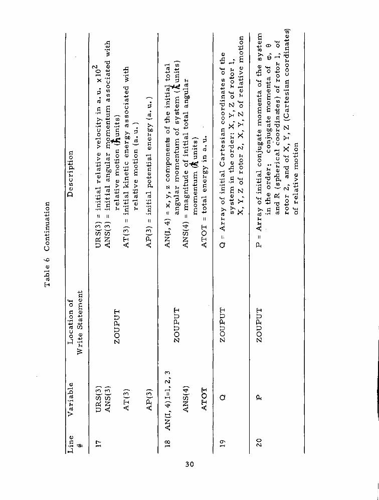
do
•|H•4->CO35
•H4^do
v£>V
i— i
•8EH
Desc
rip
tio
n
-4->d
MH O0 C
Md <u2 1o• 1— 1 VW
-4-> 4Jctf CO
g «j S
£
0)^H
,0cd
•rH
CO>
cu.s *•4
rfl•*J•I-t
£
T3(M CD -O +> ri3T3 "4^i— 1 CO .pi
= in
itia
l re
lati
ve v
elo
cit
y i
n a
. u
. x
= in
itia
l an
gu
lar
mo
men
tum
ass
oci
rela
tiv
e m
oti
on
(fj
un
its)
= in
itia
l k
ineti
c en
erg
y a
sso
cia
ted
v.
rela
tiv
e m
oti
on
(a.
u.
)
= in
itia
l p
ote
nti
al
en
erg
y (
a. u
. )
X" * --^ '
CO ro ^-- . — .
ww J2 J2pcj Z H P^D <J < <
H&PH[3oN
. . . .
2.2. m JnCO CO ^- ^
ri ^ ^p <! ^ •<
t^j__j
r-H CDCu ^j
•^J *rHo d
) =
x,
y,
z co
mp
on
ents
of
the
init
ial
tan
gu
lar
mo
men
tum
of
syst
em
(Jtu
= m
ag
nit
ud
e o
f in
itia
l to
tal
an
gu
lar
mo
men
tum
(ft
un
its)
= to
tal
en
erg
y i
n a
. u
. "
•^ — « •* H
ti co OZ, Z t^< < <
EHDkDON
CO
CM*
r-T ^T Mu ~_~ ^^
5 S §. <: •<I-H
<J
00
do•43
» ocj . C
•(-> f— 1 "
^ h s0 o >j_» »H
ray o
f in
itia
l C
art
esi
an
co
ord
inate
ssy
stem
in
th
e o
rde
r: X
, Y
, Z
of
rol
X,
Y,
Z o
f ro
tor
2,
X,
Y,
Z o
f re
lat
!H<J
I I
a
EHD&t>ON
a
0J__J
g «W t %
*> ™ "S rt-t-> a> O J!JCO "1" - - -H
« »rt "2. >-i« «« 0 Sr> o Jj °r^H ^^ ^* . .•*-> ^ o °
ray
of
init
ial
co
nju
gate
mo
men
ta o
fin
th
e o
rde
r;
co
nju
gate
mo
men
taan
d R
(sp
heri
cal
co
ord
inate
s) o
f r
roto
r 2
, an
d o
f X
, Y
, Z
(C
art
esi
an
of r
ela
tiv
e m
oti
on
JH< '
I I
k
HDPHt»0N
Pn
OCJ
30
rt0
•H•*->rt2rt
• i~t•4-1
rtoU
vO
0)I— 1
•8H
o•H•J
PH•HM
UCO
CDQ
4->
rt•« ?° ac <"2 *13 SU /i\v> <uO 4J
J '££
(1)I__[
XIrt
•HJ-t
rt>
<UC
•H =*=
I-H
!>,r^*i-H0)>
*rH
rt 4J0 to U. H D O )to u CXh C ' toCD rt 12 <u> ••-> H h
tn ort £ * N
<U CO Mtn £ rrt 0Q\ (O -*J +>
B. ^2_i r^ /T< rr-(.s rt H. 1
•o S N rt
0 ^j -> i~H
to rt w IH^ 3 'H -0 0^* _, i i ^
-l-> . "-J rt *?
§ ^ 2 * 2^H (U ^T «Ms « a x^°
i-H TO *H •H rft
3 -o M --«
1 1 1 s: I5 £ CO >s rt' d>> • — - .H n) -is- i— i
i — i .11 0 h
W o rt
5 » »>-3 H pcj
Ht)ftt)ON
W
0 H rtw1-3
i— 1
CO
a0)
-t->tns^to
<+HO
to<u
Krt <u^ T3h ho o
s srt ^rt t>
•H i— 1tow S•M rth MH
rt ^ sr-J W
Co %— -
rt•H •
MH ^m •O rt
^ rtrt ••H
^irtn
a
H&ftDON
a
COCO
r Saf- -BPQ i-, £ ;t rt
_, < ft -g n «g ^ w s ^ a5 d r O^ H ^ & g a« <! Co ri ^ .,^ ^ ^ rt _ h*" ^ - rt >-, rt.. co in o --• 'gn *ZL ** X ^ hnO e-< -fr r_ OO: < 1 1 f s25^"5 is ^ ^ 1 " §rt 0 « « - N(jj -~^ rt •*-* rt «^z; hn CL V •*-» si
*$s ^°°„-. £ rt rt ^ ""^2 1 is = u _« n,rt g, ° o a $ %fj j ^^ U M p^i^ w rt . rt M -JJft a) £ y fi -H SW S 0 £ =m VI »- o •" S S w <HF-l 0 0> « ) „ . . _
w «^3 1 ^.13 n* a «-o10 -^ o w g 'S rti to VH .,H rt !> rtA<J
S<
00Is-
H *.g gD an «U +jN rt
•r^to
ro•t
CO
I-H I— 1 • • I— 1
M CO ^-1-,
-^ ^ H CuI-H i< rj rq- <J w H1-1 ^
S<:CON
COIs-
H -s& gft S•~> "t; <u° IdN £
to
CO
co"'--i *^^"^ ^— , .. ^
TI rd^ —" ^ H £CO 2 M ft, 5 W H
I-H ^
I
<
ThCO
31
fio"S§
•H
"SoU
sO
n)
Desc
rip
tio
n
Is
° gc< Q)
1 *O njTj -Mn) W
O -Siij 'H
<JJ
nJ•|H
m
ID
•S*
rj -
« 5£ < ~"> co -£ £ <U
n <: .S0 -H
erf «>co .J <u£g^E °£n) *^ ni
bfl *•OJ g OJ
a l g2 |ad S-.g^ £ a)w S^H" ° gH « £
W n <|2
•v
CO
>
oo ^^. *-~ . "v
1 1 fO ^"^I I ^ I I1-1 to 1-1ro pcj m1-1 t-T5" §"
un00
AM
(I,
3) =
the
X,
Y,
Z c
om
po
nen
ts
of
the
fin
al a
ng
ula
r m
om
entu
m a
sso
cia
ted w
ith
the
rela
tiv
e m
oti
on
. V
R(I
, 3
) are
th
e
[H
[3PHIDON
CO CO CO
W E H P HS H W
X,
Y,
Z c
om
po
nen
ts o
f th
e fi
nal
re
lati
ve
vel
oci
ty (
a. u
. x 1
0^)
TJ
)>
PH
I(l)
are
th
e tw
o scatt
eri
ng
an
gle
s.
) d
efi
nes
the an
gle
betw
een
th
e i
nit
ial
an
rH i-H
EH EH
E EEH H
HID
IDON
i-H
<} ^T<; £!H PHEH
v£>00
t . .
fin
al r
ela
tiv
e v
elo
cit
y v
ecto
r.
PH
I(l)
def
ines
th
e d
irecti
on
of
the
co
mp
on
en
t o
J
-_r
i— r yj
HH ^
•* *•>
|
Ho 0
the f
inal
rela
tiv
e v
elo
cit
y p
erp
en
dic
ula
rth
e i
nit
ial
velo
cit
y.
AM
(I,
4),
AM
S(4
), E
are
th
e v
ari
ab
les
for
the f
inal
sta
te
H••
W
PH
co
rresp
on
din
g t
o A
N(I
, 4
),
AN
S(4
), A
TO
'fo
r th
e in
itia
l st
ate
(se
e li
ne 1
8)
riab
les
are
use
d f
or
co
nse
rvati
on t
ests
.H
FF
2,
DIF
F3
=
Th
e m
agn
itu
de
of
the
rt H
a) ?*CO fa0) fa
rC hH
H Q
rH 00
fe fafa faP P
r^00
dif
fere
nc
e b
etw
een
th
e X
, Y
an
d Z
com
po
nen
ts o
f th
e in
itia
l an
d f
inal
to
tal
ang
ula
r m
om
entu
m r
esp
ecti
vely
x 1
0£B*i2
ro Th infa fa fafa fa fa
P P P
0)a
the
mag
nit
ud
e o
f th
e d
iffe
ren
ce
betw
een
init
ial
and f
inal
mag
nit
ud
e o
f th
e to
tal
n
fa\—\
P
32
ati
nu
ati
on
oU
0)i— i<x)H
Desc
rip
tio
n
_,jr*<« s
O g
fl <yO -p4J JS
UO CD1 "^
HH »H^•4
£
<UF— 1
n)•H
td
0).s*
<orj^
CUcu
^cu
•^ooQ) OO l—l
^ c x
2 g ^3C *i i «
an
gu
lar
mo
men
tum
FF
5 =
mag
nit
ud
e o
f th
e d
iJfi
nal
an
d i
nit
ial
ene
nQ
rt
= ti
me
of
back i
nte
gra
tio
n
H
^^ro
i *~*^ *5^ cu2 a
(U-l->n)-i->CO
H
COf\3
Uoi
^3
1oCO(U
n)fi•1-1
0oU
= arr
ay
of
fin
al C
art
esi
an
inte
gra
tio
n (
see
lin
e 1
9)
a
-
a
CT^00
r^HUex)ftf-t
4nn)
(Uaoa
= arr
ay
of
fin
al
con
jug
ate
inte
gra
tio
n (
see
lin
e 2
0)
ft
-
On
£_OfO
p3UIJ.OJO.3Ci
ST UOT^BJSS^UT
^OHq T[DTHM UT S3IJ
-o^DaC^j; aoj AIUO
•
^oU
•1— injJH
UfiO
(Uft
(010(UC•1-1i— ii-t(Uao
1— I
CO<u
•H
O1 *
o<u•t— 1
(X)
£M-lO
fljCO."cuft(Uoo
n!ftfttxl
001
1— <
CO
C•H
^j.
33
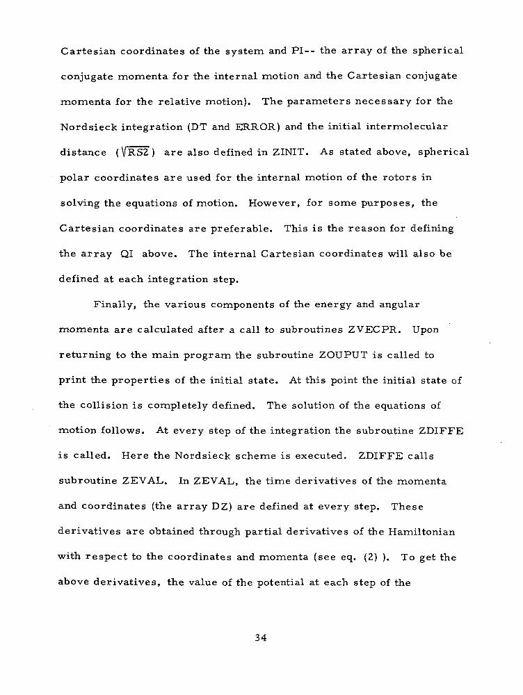
Cartesian coordinates of the system and PI-- the array of the spherical
conjugate momenta for the internal motion and the Cartesian conjugate
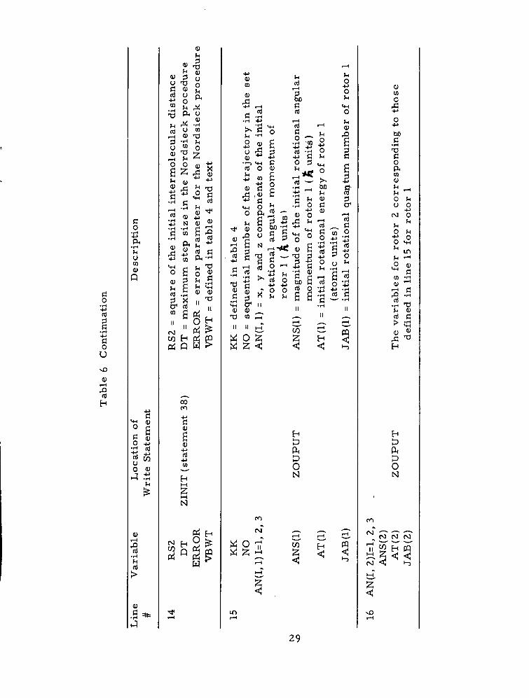
momenta for the relative motion). The parameters necessary for the
Nordsieck integration (DT and ERROR) and the initial intermolecular
distance (VRS2 ) are also defined in ZINIT. As stated above, spherical
polar coordinates are used for the internal motion of the rotors in
solving the equations of motion. However, for some purposes, the
Cartesian coordinates are preferable. This is the reason for defining
the array QI above. The internal Cartesian coordinates will also be
defined at each integration step.
Finally, the various components of the energy and angular
momenta are calculated after a call to subroutines ZVECPR. Upon
returning to the main program the subroutine ZOUPUT is called to
print the properties of the initial state. At this point the initial state of
the collision is completely defined. The solution of the equations of
motion follows. At every step of the integration the subroutine ZDIFFE
is called. Here the Nordsieck scheme is executed. ZDIFFE calls
subroutine ZEVAL. In ZEVAL, the time derivatives of the momenta
and coordinates (the array DZ) are defined at every step. These
derivatives are obtained through partial derivatives of the Hamiltonian
with respect to the coordinates and momenta (see eq. (2) ). To get the
above derivatives, the value of the potential at each step of the
34
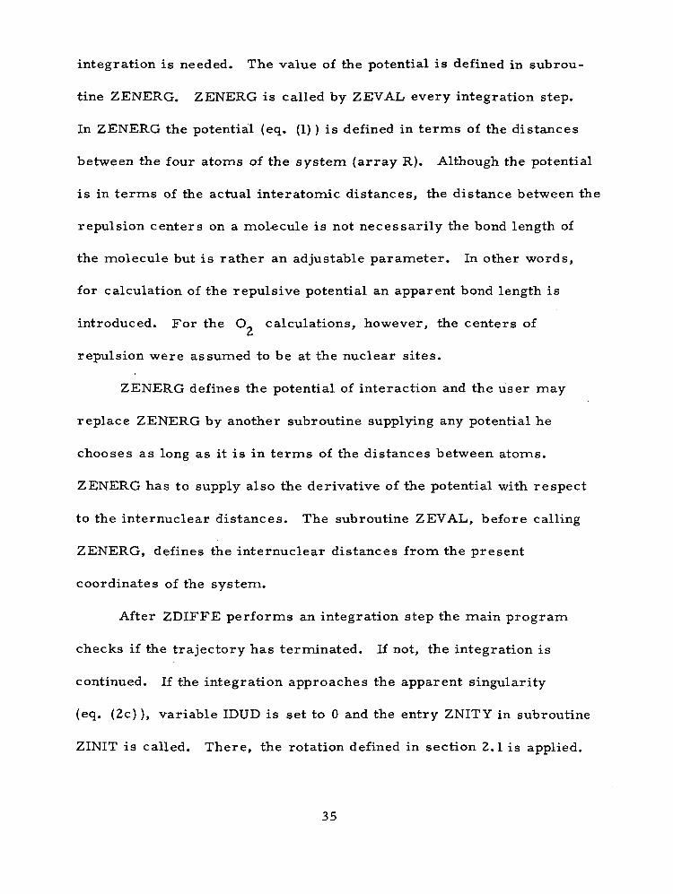
integration is needed. The value of the potential is defined in subrou-
tine ZENERG. ZENERG is called by ZEVAL every integration step.
In ZENERG the potential (eq. (1) ) is defined in terms of the distances
between the four atoms of the system (array R). Although the potential
is in terms of the actual interatomic distances, the distance between the
repulsion centers on a mol-ecule is not necessarily the bond length of
the molecule but is rather an adjustable parameter. In other words,
for calculation of the repulsive potential an apparent bond length is
introduced. For the O calculations, however, the centers ofCt
repulsion were assumed to be at the nuclear sites.
ZENERG defines the potential of interaction and the user may
replace ZENERG by another subroutine supplying any potential he
chooses as long as it is in terms of the distances between atoms.
ZENERG has to supply also the derivative of the potential with respect
to the internuclear distances. The subroutine ZEVAL, before calling
ZENERG, defines the internuclear distances from the present
coordinates of the system.
After ZDIFFE performs an integration step the main program
checks if the trajectory has terminated. If not, the integration is
continued. If the integration approaches the apparent singularity
(eq. (2c) ), variable IDUD is set to 0 and the entry ZNITY in subroutine
ZINIT is called. There, the rotation defined in section 2.1 is applied.
35
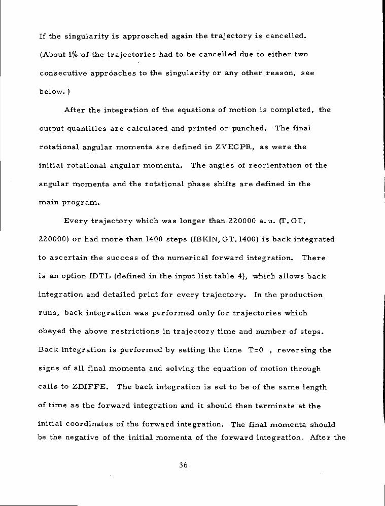
If the singularity is approached again the trajectory is cancelled.
(About 1% of the trajectories had to be cancelled due to either two
consecutive approaches to the singularity or any other reason, see
below. )
After the integration of the equations of motion is completed, the
output quantities are calculated and printed or punched. The final
rotational angular momenta are defined in ZVECPR, as were the
initial rotational angular momenta. The angles of reorientation of the
angular momenta and the rotational phase shifts are defined in the
main program.
Every trajectory which was longer than 220000 a. u. (T.GT.
220000) or had more than 1400 steps (IBKIN, GT. 1400) is back integrated
to ascertain the success of the numerical forward integration. There
is an option IDTL (defined in the input list table 4), which allows back
integration and detailed print for every trajectory. In the production
runs, back integration was performed only for trajectories which
obeyed the above restrictions in trajectory time and number of steps.
Back integration is performed by setting the time T=0 , reversing the
signs of all final momenta and solving the equation of motion through
calls to ZDIFFE. The back integration is set to be of the same length
of time as the forward integration and it should then terminate at the
initial coordinates of the forward integration. The final momenta should
be the negative of the initial momenta of the forward integration. After the
36
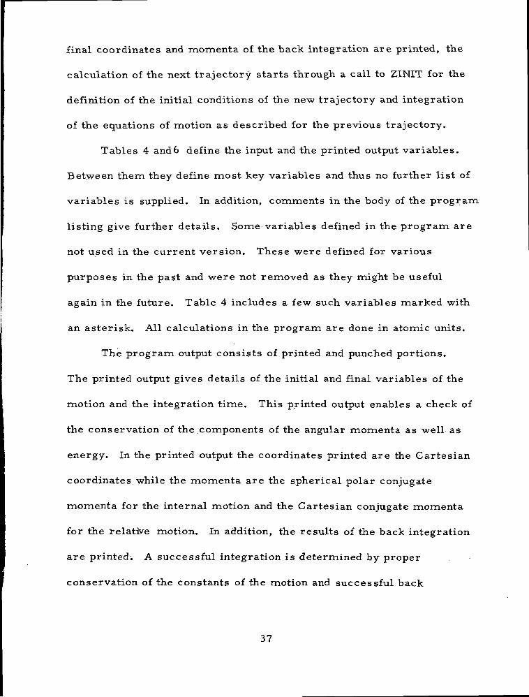
final coordinates and momenta of the back integration are printed, the
calculation of the next trajectory starts through a call to ZINIT for the
definition of the initial conditions of the new trajectory and integration
of the equations of motion as described for the previous trajectory.
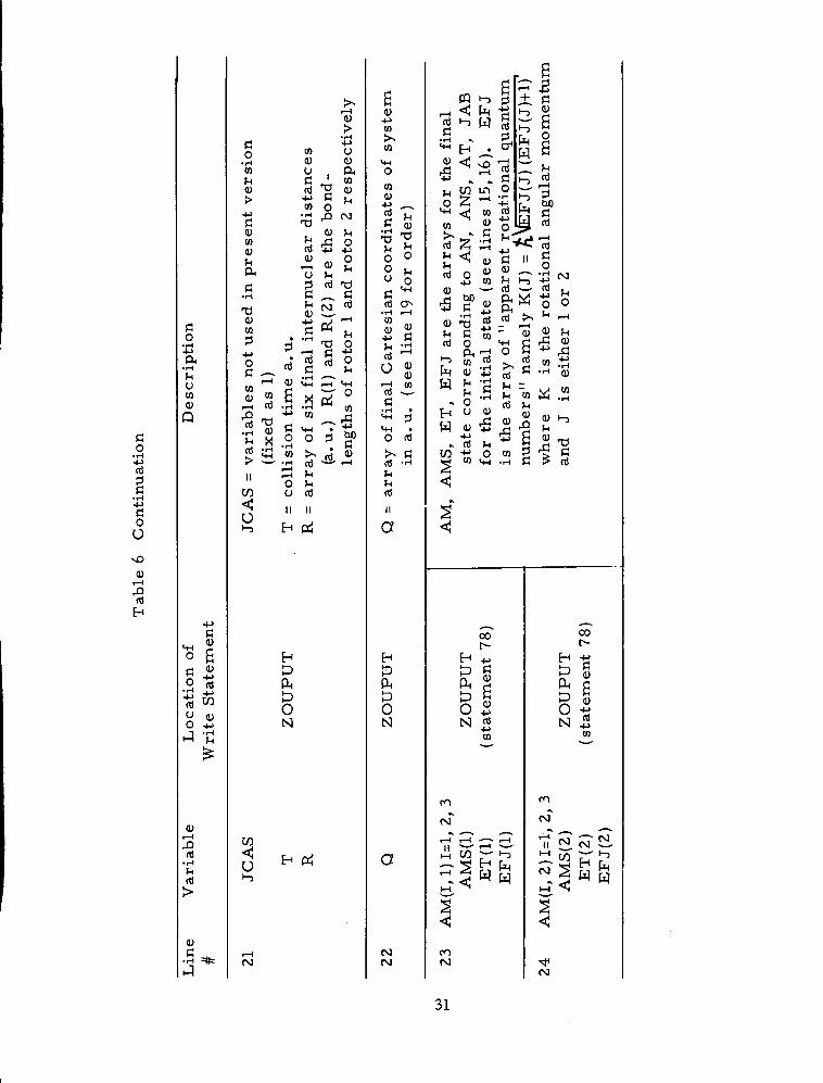
Tables 4 and6 define the input and the printed output variables.
Between them they define most key variables and thus no further list of
variables is supplied. In addition, comments in the body of the program
listing give further details. Some variables defined in the program are
not used in the current version. These were defined for various
purposes in the past and were not removed as they might be useful
again in the future. Table 4 includes a few such variables marked with
an asterisk. All calculations in the program are done in atomic units.
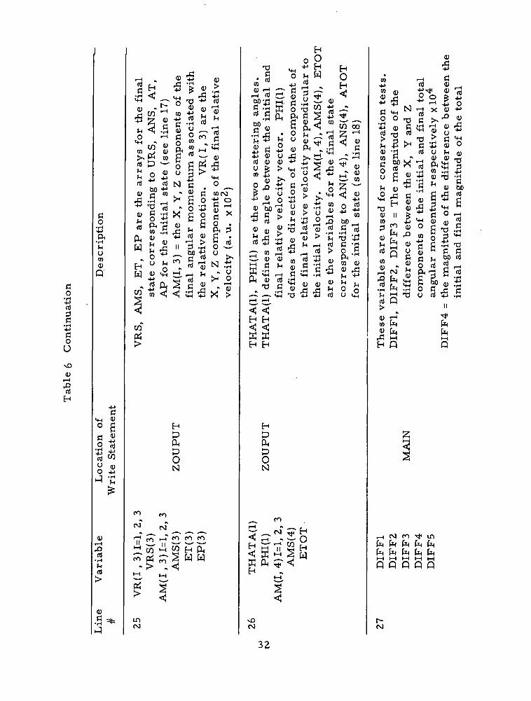
The program output consists of printed and punched portions.
The printed output gives details of the initial and final variables of the
motion and the integration time. This printed output enables a check of
the conservation of the components of the angular momenta as well as
energy. In the printed output the coordinates printed are the Cartesian
coordinates while the momenta are the spherical polar conjugate
momenta for the internal motion and the Cartesian conjugate momenta
for the relative motion. In addition, the results of the back integration
are printed; A successful integration is determined by proper
conservation of the constants of the motion and successful back
37
integration. A successful back integration was taken to mean that no
coordinate or momentum, after back integration, differs by more than
_22 X 10 a. u. from its initial value. Any trajectory which failed in
integration was repeated with tighter integration parameters. As
mentioned above, about 1% of the trajectories were not accepted due to
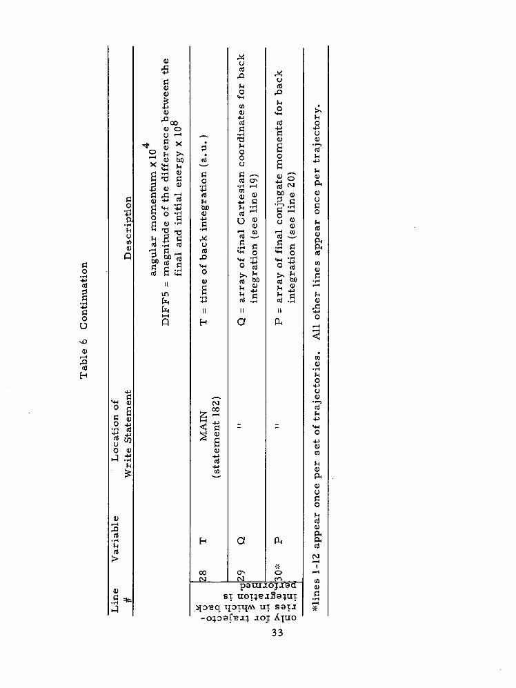
repeated failures of the integration from any cause. Table 6 describes
the printed output.
The punched output (a sample of which is reproduced in table 3)
includes the initial and final properties of each collision necessary for
the calculation of various properties and cross sections (e.g. Gordon,
1968). The properties included in the punched output are: W,_._(T ) --V13 1
defined in section 2. 2; cos a -- the cosine of the angular change in the
orientation of the rotational angular momentum vector of a rotor in the
collision; K. -- the initial angular momentum; K -- the final angular
momentum; cos v , sinv , cos 2v , sin 2v , which are the average
values of the sine and cosine of the classical rotational phase shift (v)
and of 2v respectively, and V the relative initial velocity. The
cosines and sines of both v and 2v are given since the values for
these trigonometric functions are averages of two possible values as
defined in the end of section 2.1. The averages for 2v cannot be
derived directly from the averages for v (e. g. F(v) = cos 2v)
38
Since there are in the case of O -O collisions two identicalLi L*
molecules per collision, each trajectory yields 2 sets of output. These
appear in the two consecutive cards (or lines in table 3 ) with the same
value for W,.._.(Tn) . In converting to different temperatures, it is theV 13 1
rotational angular momentum of the perturbing molecule in a set of two
colliding molecules which corresponds to G(J.T) in equation (20).
3. USE OF THE PROGRAM: O CALCULATIONS
The general usefulness of the data derived from the above pro-
gram for a set of individual trajectories is in the fact that different
properties can be calculated after the most complicated and computer -
time consuming calculations, (namely the four-body trajectory calcula-
tions) are done. Expressions for various cross sections necessary for
the elucidation of a number of properties are given by Gordon (1968 and
1967). The expressions in this section (equations (21)-(23)) are also
derived in these last references. The calculations performed on the
O molecule microwave spectrum are described in the following toCi
demonstrate one use of the data derived from the above program.
The loss tangent can be defined as
. . . 4nnu) _ , . . -1 , . ,,tan 6 (<u) = -r Imd . (g - ^ - ivpg) . g.d = A-K (21)
A is the absorption coefficient, K is the wavelength/2TT , n is the
number density of the absorbing molecule, p is the number density of
39
the perturbing molecule, k is the Boltzmann constant and jo is the
angular frequency of the radiation times the unity matrix. T is the
absolute temperature, d is a vector of all the magnetic dipole/•^
moment matrix elements, p is a diagonal matrix of the probabilities«w
of the various molecular states, v is the mean relative velocity and
<j is a relaxation matrix to be discussed below. All quantities exceptK
for a are well known. The diagonal elements of a have the following£3 £3
interpretation:
-ImpvCT. . = line shift11
R e p v c r . . = line width11
(22)
for line i . For the O microwave spectrum the line shift parameterL*
equals zero as CT is a real matrix. One can express cr as^3 £3
CO
= v -1 f 2rrBd B < v(l - S) > (23)/ v« « x
where B is the impact parameter; v is the relative velocity; v is
the mean relative velocity; S is a collisional transfer matrix for aw
single collision; and the brackets indicate average overall collisions
with the same impact parameter.
40
A matrix element of the S matrix S.. defines the amplitudew ij ^
transferred from spectral line j to spectral line i in a collision.
(See Gordon, 1967, for the derivation and definition of the S matrix.
Note, however, that the above S matrix does not define transitions' ' w
between states as does the familiar scattering matrix. ) The microwave
spectrum of O in the frequency region discussed below is a multiplet£
spectrum, and thus every line arises from transitions between states,
both with the same molecular rotational quantum number. Hence, each
line can be assigned to a rotational level. The elements of the S
matrix will be, therefore, a product of the probability of transition
between the initial and final rotational level and another term defining
the probability of transition between the various multiplet lines
corresponding to each rotational level (Gordon, 1967). If we define
f(V, B, J) in equation (20) to be 5..- S.. , equation (23) can be solvedJ J
using equation (20) and the calculated set of trajectories (the trajecto-
ries are completed as defined in section 2.1). A submatrix of 1 - Sr « «
corresponding to the lines belonging to one rotational level of O isL*
reproduced in table 1 from Gordon (1967). The variable Pf. in table 1
is defined as probability of transfer in a particular collision from the
initial rotational level i to some final rotational level f and a is
defined as the angle of reorientation of the rotational angular momentum
in a collision.
41
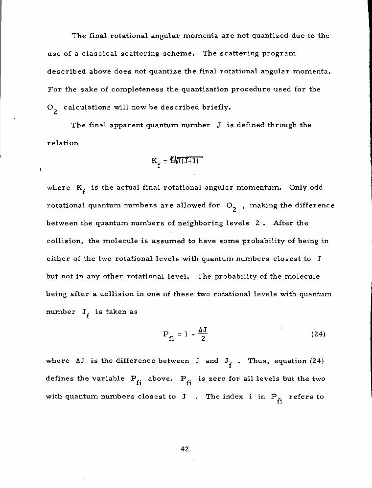
The final rotational angular momenta are not quantized due to the
use of a classical scattering scheme. The scattering program
described above does not quantize the final rotational angular momenta.
For the sake of completeness the quantization procedure used for the
O calculations will now be described briefly.£*
The final apparent quantum number J is defined through the
relation
Kf =
where K is the actual final rotational angular momentum. Only odd
rotational quantum numbers are allowed for O , making the differenceC*
between the quantum numbers of neighboring levels 2 . After the
collision, the molecule is assumed to have some probability of being in
either of the two rotational levels with quantum numbers closest to J
but not in any other rotational level. The probability of the molecule
being after a collision in one of these two rotational levels with quantum
number J is taken as
where AJ is the difference between J and J . Thus, equation (24)
defines the variable P.. above. P.. is zero for all levels but the twofi fi
with quantum numbers closest to J . The index i in P refers to
42
the initial rotational level in the collision which is well defined by the
sampling procedure (see section 2. 2).
A detailed discussion of the O microwave computations and theL*
comparison of experimental results to calculations are given by
Mingelgrin (1972). Note that there are no adjustable parameters in this
theory and that the potential parameters are derived from independent
data (see section 2.1).
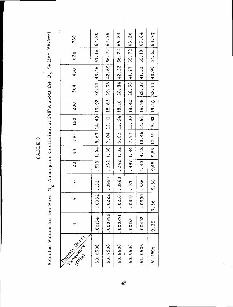
Some results are given in figures 1-4 and tables 7 and 8. Table
7 gives the calculated line width parameters for the different lines and
compares them to experimental results. There are two absorption
lines, designated J-t- and J- , per rotational level. The wide varia-
tion in the experimental results makes the comparison with them diffi-
cult. This points out the need for further study of the O spectrum atLJ
low densities. Since the scattering calculations reported here are
classical, the line width parameters for the lowest rotational level
should have the largest error.
2A set of programs developed by R. G. Gordon's group at Harvard
University designed to evaluate expressions of the form of equation
(21) from results of scattering calculations, such as described above,
was used to derive the following results.
43
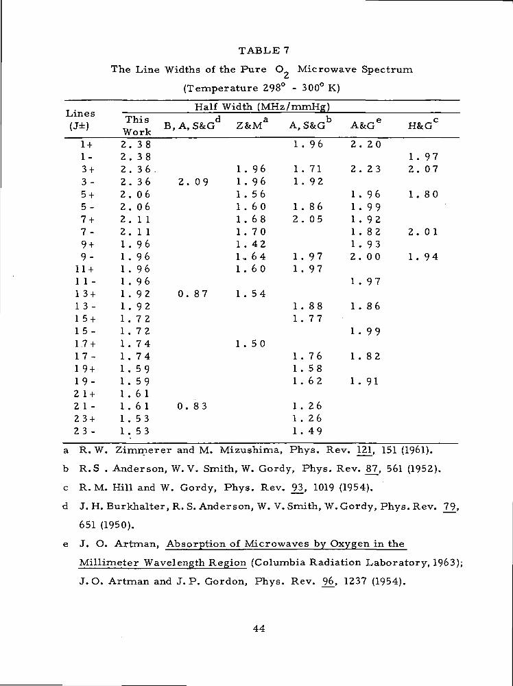
TABLE 7
The Line Widths of the Pure O Microwave Spectrum
(Temperature 298° - 300° K)
Lines
(J±)
11111111112222
1 +1-3 +3 -5 +5-7 +7 -9 +9-1 +1 -3 +3 -5 +5 -7 +7 -9 +9-1 +1 -3 +3 -
Half Width (MHz/mmHR)This d aWork ' '2.2.2.2.2.2.2.2.1.1.1.1.1.1.1.1.1.1.1 .1.1.1.1.1.
333300119999997777556655
886 .6 2. 09661166662 0. 87222449911 0 . 8 333
1 .1 .1 .1 .1 .1.1 .1,.1.
1 .
1 .
969656606870426460
54
50
A, S&Gb
1 .
1 .1.
1 .2.
1 .1 .
1 .1 .
1 .1 .1.
1 .1 .1.
96
7192
8605
9797
8877
765862
262649
A&G6
2.
2.
1 .1.1 .1 .1 .2.
1 .
1 .
1 .
1 .
1.
2 0
23
969992829300
97
86
99
82
91
H&G°
1. 972. 07
1 . 8 0
2. 01
1. 94
a R. W. Zimmerer and M. Mizushima, Phys. Rev. 121, 151 (1961).
b R.S . Anderson, W. V. Smith, W. Gordy, Phys. Rev. 87, 561 (1952).
c R. M. Hill and W. Gordy, Phys. Rev. 93, 1019 (1954).
d J. H. Burkhalter, R. S. Anderson, W. V. Smith, W. Gordy, Phys. Rev. 79,
651 (1950).
e J. O. Artman, Absorption of Microwaves by Oxygen in the
Millimeter Wavelength Region (Columbia Radiation Laboratory, 1963);
J. O. Artman and J. P. Gordon, Phys. Rev. 96, 1237 (1954).
44
6x
CO
W
+(T-
00
O
0)
o00
oo
c0)
0)
OU
OCO
ooorH
£
t-to
0r-Hrt
0)-(->U0)
i-Ha;en
oxDf^-
OOOxO
0in"xf
^HOCO
oo00
om^
o0i-H
o
o00
oi-H
m
i-H
<£/O /\^y / f\
1 / £j»
$//^
£*?y <£* >$/V Q
o00.
r —xO
CO
.
[ —in
xOi — i,CO
^f
00! 1
0CO
000s
t
Qsi-H
o^"xf
^
1 — 1
OOxD
00
•r-H
oor-Hin
00COi-H
OOroCO0
9
•xf
OO
xOoinxO
OxO
inCO,t-xO
i-H
•
xOm
xO,
00^fxDCO.
QX00
COxO
,
ooi— i
, — i^
oor-H
^fO
r-^
CO
i — ioomCO
r-00000
000000o
•
mooo00
vOoin
dxO
^00.
xDxO
oo«
xOin0000
•
00^•xf00.
00oo
xDi-H
ooi-H
•xfin
900i — i
roooxO
00CO
•i-H
ooCO
COxOooo
xO1 — 100o
•
i-Ht^000oo
xOoinoooxO
xOoo.xOxO
001 -,
inm
f^
^fxOm.oo00
00^f
•oor-H
OCO
^COr-H
f-
t^
00•
i-H
^f
00I— 1
I — 1COo
•
00oo
xOoin
oxO
xD.
mxO
oor-H
mm
COCO
r-H
[s-
ro.
0000
00ON
4
00i-H
xDxO
^f
xD
O
00r-H
0
•1— 1
xD00CO
O
O^0
00o0o
*
xO0moi-HxO
^o,
vO
r-4vO
%
Tjl
LO
O»
0-*•xfI — 1
co00
xOi-H
Qxi— 1
C4CO
^mi — i
0t-H
OOi-H
CO
00
00
*
xOCO
inCO
c>
xOomi— ii-HxO
45
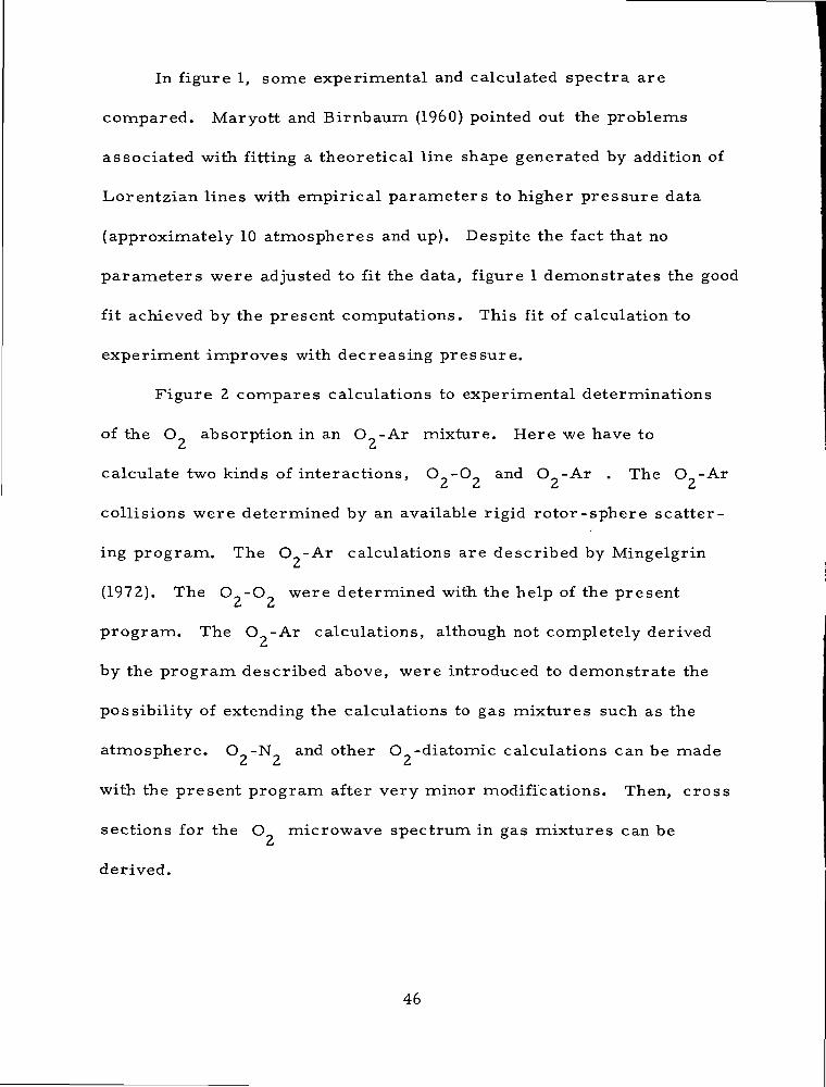
In figure 1, some experimental and calculated spectra are
compared. Maryott and Birnbaum (I960) pointed out the problems
associated with fitting a theoretical line shape generated by addition of
Lorentzian lines with empirical parameters to higher pressure data
(approximately 10 atmospheres and up). Despite the fact that no
parameters were adjusted to fit the data, figure 1 demonstrates the good
fit achieved by the present computations. This fit of calculation to
experiment improves with decreasing pressure.
Figure 2 compares calculations to experimental determinations
of the O absorption in an O -Ar mixture. Here we have to£* L*
calculate two kinds of interactions, O -O and O -Ar . The O -ArCj LJ LJ L*
collisions were determined by an available rigid rotor-sphere scatter-
ing program. The O -Ar calculations are described by Mingelgrin
(1972). The O -O were determined with the help of the presentL* Li
program. The O -Ar calculations, although not completely derivedLJ
by the program described above, were introduced to demonstrate the
possibility of extending the calculations to gas mixtures such as the
atmosphere. O -N and other O -diatomic calculations can be madeCi L* L*
with the present program after very minor modifications. Then, cross
sections for the O microwave spectrum in gas mixtures can be
derived.
46
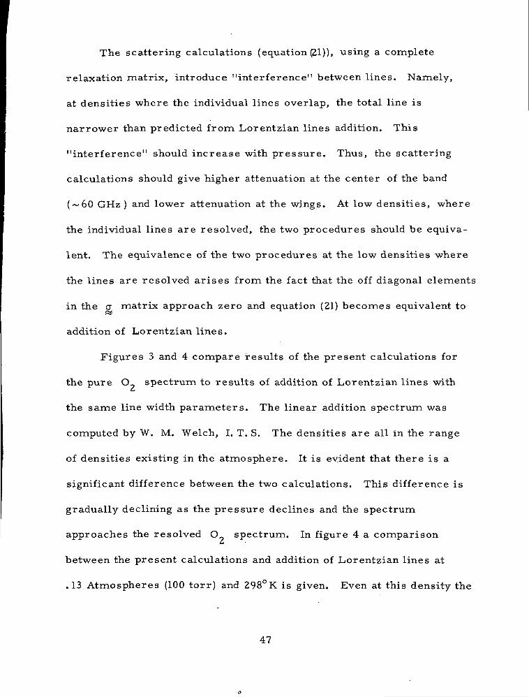
The scattering calculations (equation (21)), using a complete
relaxation matrix, introduce "interference" between lines. Namely,
at densities where the individual lines overlap, the total line is
narrower than predicted from Lorentzian lines addition. This
"interference" should increase with pressure. Thus, the scattering
calculations should give higher attenuation at the center of the band
(~60 GHz ) and lower attenuation at the wings. At low densities, where
the individual lines are resolved, the two procedures should be equiva-
lent. The equivalence of the two procedures at the low densities where
the lines are resolved arises from the fact that the off diagonal elements
in the a matrix approach zero and equation (21) becomes equivalent to
addition of Lorentzian lines.
Figures 3 and 4 compare results of the present calculations for
the pure O_ spectrum to results of addition of Lorentzian lines with
the same line width parameters. The linear addition spectrum was
computed by W. M. Welch, I. T. S. The densities are all in the range
of densities existing in the atmosphere. It is evident that there is a
significant difference between the two calculations. This difference is
gradually declining as the pressure declines and the spectrum
approaches the resolved O spectrum. In figure 4 a comparison£j
between the present calculations and addition of Lorentzian lines at
.13 Atmospheres (100 torr) and 298°K is given. Even at this density the
47
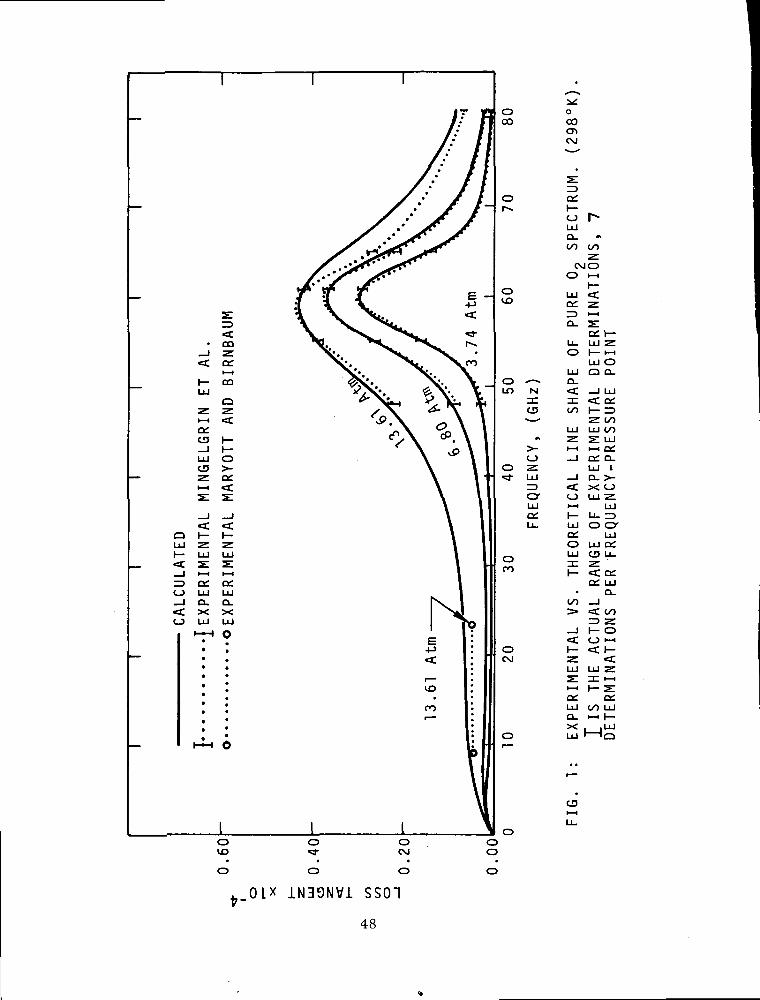
1o00
C\J
Or
LUD- "oo oo
z.CMO
O >-i
LJ_ UJ O f— I-H
UJ OLU O Q.Q.<C —I LiJz <: o:
uj uj oo•z. s: ujI— I I— I Qi
_j o: Q-LU i
—I Q- >-< x: o
uj o crQi UJO LU a:LU CD Ll_
C£ LUD.
^ _1> <C 00
^) Z— 1 1 — 0<=c o i— i
a: a:LU oo LUa. K-. t—X | |LULU I 'a
CD
O O
1N39NV1 SS01
48
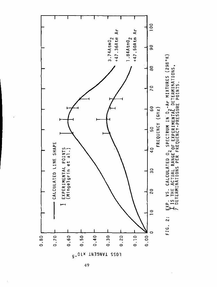
CM EO 4->E <C
-!-> VO<: co
co
CM EO •!->E <C
•»-> O<: m^t-oo r .
• •=!•r- +
OO
OCO
oCOCT> «CM OO••- z
oOO "—«
•=> z oo0 v- »-i t—'*- x 2: z
i—i o: i—isi uj o
I— Q.X- LUet Q LU
O ^ I OHVO N CM—I =3
3T O «Ct/0o . I—oo
Z ZLUi—i LUQ:
oLO
LUO
crLU01
O XLULU LUZDo. o-oo LULU
OQCCM U_
O LU
oco
oCsl
LUI— Od<f. oo_l — 1Z^ <CO
o•
ooLU
• OOLUO_ >—i Q
CM
•
CD
oCO
or^.
O
oVO
oCO
oCM
o•
o
oo
01* 1N39NV1 SS01~
49
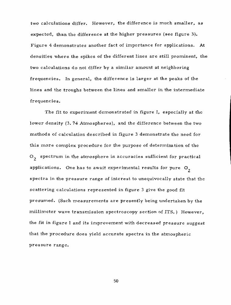
two calculations differ. However, the difference is much smaller, as
expected, than the difference at the higher pressures (see figure 3).
Figure 4 demonstrates another fact of importance for applications. At
densities where the spikes of the different lines are still prominent, the
two calculations do not differ by a similar amount at neighboring
frequencies. In general, the difference is larger at the peaks of the
lines and the troughs between the lines and smaller in the intermediate
frequencies.
The fit to experiment demonstrated in figure 1, especially at the
lower density (3. 74 Atmospheres), and the difference between the two
methods of calculation described in figure 3 demonstrate the need for
this more complex procedure for the purpose of determination of the
O spectrum in the atmosphere in accuracies sufficient for practicalLJ
applications. One has to await experimental results for pure OL*
spectra in the pressure range of interest to unequivocally state that the
scattering calculations represented in figure 3 give the good fit
presumed. (Such measurements are presently being undertaken by the
millimeter wave transmission spectroscopy section of ITS. ) However,
the fit in figure 1 and its improvement with decreased pressure suggest
that the procedure does yield accurate spectra in the atmospheric
pressure range.
50
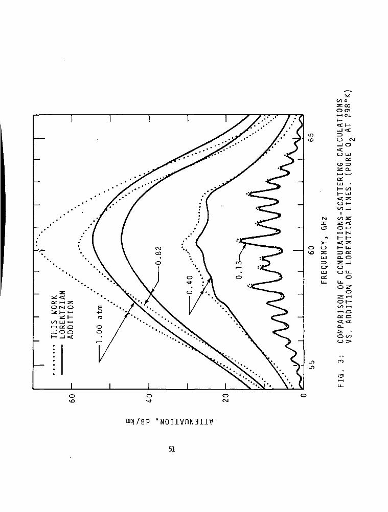
OIL i—i Z:O M O
CO LiJ H-ii—i OL Orc o o
CO oz ooo enI-H OJ
<_> O—J O«£CJ LU
o:CD ^>•z. a.
00
O 1-1co _i
iN co z:in z: <:CD O •-•
t-i M
O O h- UJco z: ZD oi
LLJ O_ Ors s: -Jcr oUJ C_3 U_Od OL LJ_
o -z.o
O I—CO I—Ii—i Orv t—\
Q.s: •O CO
LO
CO
CD
O10
oCM
'NOiivnN3iiv
51
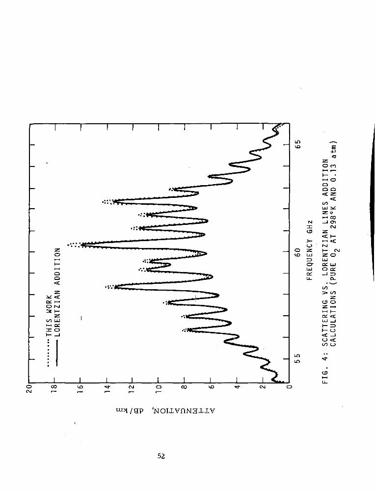
oo
00 LUI—l Qln: o
LO
Nln:CD
>-O
o zVO LU
^3crLU
intn
4Jto
zO CO
1-1 Ooa o<c z
<cooLU ^Z OI-H 00
_l CTtCM
IVlh- CMZ OLUcc: LUo a:_J Z3
a.
oo> oo
CD OZ •— i1-1 h-o; <:LU _il— ^I— o«c —io <coo o
CJ
oC\J
CO CVJ 00 CVJ
52
It may seem that the equivalent of the scattering procedure can
be achieved by adding Lorentzians with pressure dependent shift and
width parameters. This is exactly so, except that the procedure
described here does not rely on an empirical fit. As such, the method
is universal and enables calculations of complete frequency or density
profiles. Empirical fit of pressure dependent width and shift para-
meters will depend on the accuracy of available measurements and will
be applicable only to a small range of conditions as determined by the
experimental points to which the parameters are fitted.
Finally, the dispersion spectrum of O at the microwave region
can be easily computed using the same information and programs used
for computation of the absorption spectrum. The r-eal part of the
refractive index at frequency uu (n(u))) can be obtained from the relation
P d (25)tt f^f
where all symbols have the same meaning as in equation (21). Equation
(25) is discussed more fully in a forthcoming paper by the author. This
equation may not apply at sufficiently high density, but it certainly
holds for all pressures around and below 1 Atmosphere at 298°K. Some
results of dispersion calculations are given in figures 5 and 6.
53
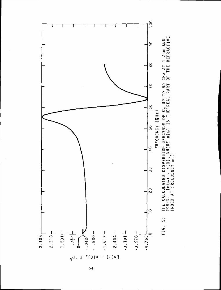
,01 X [ ( 0 ) " - (<")"]
54
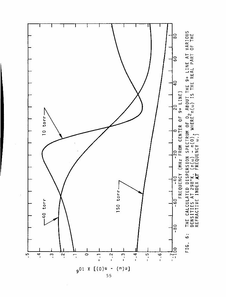
oCO
<: o:LU Q-•z.t—i _J—i <:
LU+ OL
+ <:•CTi
CSJO LU
o;
o I— o 3
s: LUO O.
o o: coCM u.I Z
C >-O
N
coC£«LUQ-co
3 cr--- LU
c oc:
cr QLU LUOL I—
o10
O00 Xcn LUCM Q
LUCOLU 1t-l I—h- Oi— i <CCO Qi
O LU 1— i
<CO
LO <* CO CM i— O i—
oCO
Oo
i— Q Q:
CM CO LO
X [ ( 0 ) " - ( ( T ) )u ]55
Zeeman splitting was neglected in all the computations. This,
however, will affect the calculations at 298°K and pressures above 5 torr
only negligibly for magnetic field strengths below or around . 5 Gauss
which is approximately the strength of the earth's magnetic field
(Liebe and Welch, 1972).
4. ACKNOWLEDGMENTS
We would like to thank Dr. R. G. Gordon for the use of his
integral transformation procedure for the selection of the initial
conditions, and W. M. Welch for the use of his calculated spectrum.
We also wish to thank Dr. J. Cooper for his thorough review of this
report, and to Mrs. J. Trebing for her meticulous typing of the manuscript.
56
5. REFERENCES
Anderson, P. W. , (1949), "Pressure broadening in the microwave andInfra-Red regions," Phys. Rev., 76, 647-661.
Conroy, H. , (1967), "Molecular Schrodinger equation III. A newmethod for the evaluation of multidimensional integrals, "J. Chem. Phys. 47, 5307-5318.
Goldstein, H. , (1950), "Classical Mechanics, " Addison-WesleyPublishing Co. , inc. , 399 pp.
Gordon, R. G. , (1966), "Theory of the width and shift of molecularspectral lines in gasses, " J. Chem. Phys. 44, 3083-3089.
Gordon, R. G. , (1967), "On the pressure broadening of molecularmultiplet spectra," J. Chem. Phys. , 46, 448-455.
Gordon, R. G. , (1968), "Correlation functions for molecular motion, "Adv. Mag. Res. ^, 1-42.
Karplus, M. , R. N. Porter, and R. D. Sharma, (1965), "Exchangereactions with activation energy. I simple barrier potential for(rLH )," J. Chem. Phys. , 43_, 3259-3287.
J. C*
Liebe, H. J. , and W. M. Welch, (1972), "Analysis of molecularattenuation and phase dispersion between 40 and 140 GHz for slantpath models at various altitudes, " OT/ITS Report in preparation.
London, F. , (1942), "On centers of Van Der Waals Attraction, "J. Phys. Chem, 46, 305-316.
Maryott, A. A. , and G. Birnbaum, (I960), "Microwave absorption incompressed O ," J. Chem. Phys. 32, 686-691.
Mingelgrin, U. , (1972), "The pressure broadening of the O« micro-wave spectrum," Ph.D. thesis, Harvard University,Cambridge, Mass.
57
Mingelgrin, U. , R. G. Gordon, L. Frenkel and T. E. Sullivan, "Themicrowave spectrum of compressed C>2 and C^-foreign gasmixtures at the 48-81 GHz region, " accepted for publication byJ. Chem. Phys.
Nordsieck, A. , (1962), "On numerical integration of ordinarydifferential equations, " Math. Comp. 16, 22-49.
58GPO 843 • 534