Embed Size (px)
Citation preview

Post
Scri
pt⟩ p
roce
ssed
by
the
SLA
C/D
ESY
Lib
rari
es o
n 29
Mar
199
5.H
EP-
TH
-950
3211
UICHEP-TH/95-1
hep-th/9503211
Integrable Lax Hierarchies, their Symmetry Reductionsand Multi-Matrix Models 1
H. Aratyn2
Department of Physics
University of Illinois at Chicago
845 W. Taylor St.
Chicago, IL 60607-7059
e-mail: [email protected]
Abstract
Some new developments in constrained Lax integrable systems and their applications
to physics are reviewed. After summarizing the tau function construction of the KP
hierarchy and the basic concepts of the symmetry of nonlinear equations, more re-
cent ideas dealing with constrained KP models are described. A unifying approach to
constrained KP hierarchy based on graded SL(r+n; n) algebra is presented and equiv-
alence formulas are obtained for various pseudo-di�erential Lax operators appearing in
this context.
It is then shown how the Toda lattice structure emerges from constrained KPmodels
via canonical Darboux-B�acklund transformations. These transformations enable us to
�nd simple Wronskian solutions for the underlying tau-functions.
We also establish a relation between two-matrix models and constrained Toda lat-
tice systems and derive from this relation expressions for the corresponding partition
function.
1Lectures presented at the VIII J.A. Swieca Summer School, Section: Particles and Fields, Rio de Janeiro- Brasil - February/95
2Work supported in part by the U.S. Department of Energy under contract DE-FG02-84ER40173

Contents
1 Introduction 1
1.1 Abbreviations; Diagram of Lectures : : : : : : : : : : : : : : : : : : : : : : : 1
1.2 Content of Lectures : : : : : : : : : : : : : : : : : : : : : : : : : : : : : : : : 2
1.3 Acknowledgements : : : : : : : : : : : : : : : : : : : : : : : : : : : : : : : : 4
2 Pseudo-di�erential Operators, BA Functions and Hirota Equations 5
2.1 Lax Equation and Eigenfunction for the Lax Operator : : : : : : : : : : : : 5
2.2 Conservation Laws of KP Hierarchy, and Tau-Function Representation of the
Baker-Akhiezer Function : : : : : : : : : : : : : : : : : : : : : : : : : : : : : 5
2.3 Dressing Operator : : : : : : : : : : : : : : : : : : : : : : : : : : : : : : : : : 8
2.4 Hirota Equations : : : : : : : : : : : : : : : : : : : : : : : : : : : : : : : : : 9
2.5 Hamiltonian Densities and the � -Function : : : : : : : : : : : : : : : : : : : 10
3 Symmetry Reduction of the Integrable Systems. Five Constructions of the
CKP models. 12
3.1 Symmetry of Nonlinear Evolution Equation : : : : : : : : : : : : : : : : : : 12
3.2 Symmetry Reduction and the CKP Hierarchy : : : : : : : : : : : : : : : : : 133.3 CKP Hierarchy as SL(m;n)-type Lax Hierarchy and its Bi-Poisson Structure 183.4 A�ne sl(n+ 1) Origin of SL(n+ 1; n) CKP Hierarchy. : : : : : : : : : : : 22
4 Darboux-B�acklund Techniques of SL(p; q)CKP Hierarchies and Constrained
Generalized Toda Lattices 26
4.1 Emergence of the Toda structure from Two-Bose KP System : : : : : : : : : 264.2 On the DB Transformations of the SL(r + n; n) CKP Lax Operators : : : : 28
4.3 DB Transformation and Eigenfunctions of the Lax Operator : : : : : : : : : 294.4 Exact Solutions of SL(p; q) CKP hierarchy via DB Transformations : : : : : 304.5 Relation to the Constrained Generalized Toda Lattices : : : : : : : : : : : : 324.6 Darboux-B�acklund Transformation and the Dressing Chain. : : : : : : : : : 334.7 Connection to Grassmannian Manifolds and n-Soliton Solution for the KP
Hierarchy : : : : : : : : : : : : : : : : : : : : : : : : : : : : : : : : : : : : : 35
5 Two-Matrix Model as a SL(r + 1; 1)-CKP Hierarchy 36
5.1 Two-Matrix model, Orthogonal Polynomials Technique : : : : : : : : : : : : 36
5.2 Two-Matrix Model as a Discrete Linear System : : : : : : : : : : : : : : : : 375.3 String Equation : : : : : : : : : : : : : : : : : : : : : : : : : : : : : : : : : : 395.4 Partition Function of the Two-Matrix String Model : : : : : : : : : : : : : : 43
A Schur Polynomials 44
B Wronskian Preliminaries 44
1
1 Introduction
1.1 Abbreviations; Diagram of Lectures
Abbrevations used in text:
KP hierarchy (equation)= Kadomtsev-Petviashvili hierarchy (equation)
CKP hierachy = constrained KP hierarchy
DB transfromation = Darboux-B�acklund transfromation
KdV hierarchy (equation)= Korteveg-de Vries hierarchy (equation)
BA function= Baker-Akhiezer function
AKNS hierarchy = Ablowitz-Kaup-Newell-Segur hierarchy
AKS approach = Adler-Kostant-Symes approach
GNLS equation= generalized non-linear Schr�odinger equation
KP Hierarchy 2-Matrix Model
? ?
sl(r + n; n) CKP
sl(r) KdV
constr. Toda Lattice-DB
transformation
symmetry constraint string equation
-� -� -�
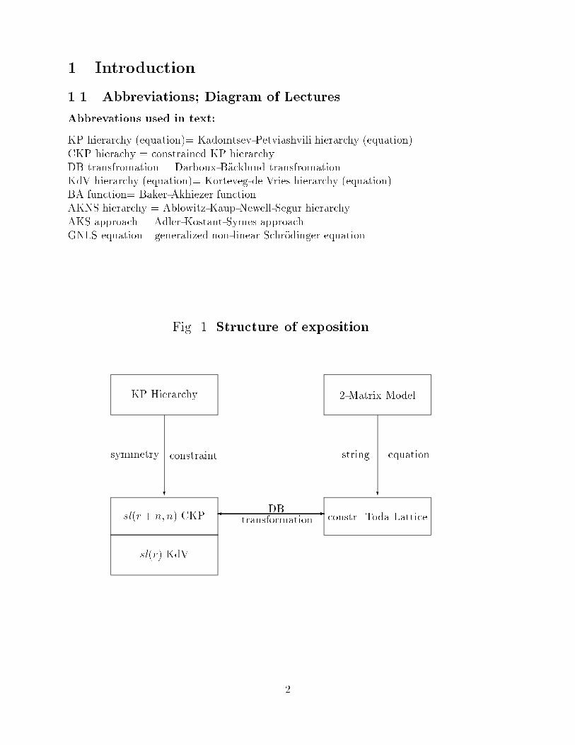
Fig. 1. Structure of exposition
2

1.2 Content of Lectures
In these lectures we study constrained KP hierarchy, its connection to the discrete Toda
models and application via Toda models to the multi-matrix approach to the two-dimensional
gravity.
A presentation follows the diagram shown on the previous page in the counter-clockwise
direction. In Section 2 we collect some standard facts on KP hierarchy which are used in
several places in these lectures. A link between the BA function and � function is estab-
lished and it is shown how to obtain the conserved current densities of the KP hierarchy
from these concepts. A complementary presentation of KP hierachy centered around multi-
Hamiltonian/Poisson structures was given at the previous Swieca school [6].
The notion of constrained KP hierarchies is introduced in Section 3. Since this notion
is signi�cant for our lectures we introduce a variety of reduction schemes and elaborate on
their mutual equivalency.
The picture which emerges from this discussion is most simply presented in the languageof pseudo-di�erential operators. Two basic equivalent approaches look especially attractiveand deserve to be mentioned here in the introduction.
One construction introduces the Lax operator of the constrained KP (CKP) hierarchy as
a ratio
Lm;n �L(m)
L(n)n � m� 1 (1.1)
of two purely di�erential operators
L(m) = (D + vm) (D + vm�1) � � � (D + v1) ; L(n) = (D + ~vn) (D + ~vn�1) � � � (D + ~v1)(1.2)
with coe�cients vi; ~vi subject to a constraint:
mXj=1
vj �nXl=1
~vl = 0 (1.3)
Imposing condition (1.3) is equivalent to requiring tracelessness of the underlying gradedSL(m;n) algebra. For this reason we refer to this class of constrained KP (CKP) models asSL(m;n) CKP hierarchy. This construction is useful to describe a bi-Poisson structure of
the CKP hierarchy and in fact involves variables which almost abelianize the second Poisson
structure. There is another formulation of the same class of models which is based on analternative expression for the Lax operator given in (1.1):
Lm=r+n;n = Dr +r�2Xl=0
ulDl +
nXi=1
�iD�1i (1.4)
A connection between variables from (1.1) and (1.4) takes a form of complicated Miura-like
transformations ( see Section 3 and [12]), but for i's the link is very simple since i's turn
out to be elements of the n-dimensional kernel of L(n). Furthermore �i;i abelianize the�rst bracket structure. Their property of being eigenfunctions of Lr+n;n makes the expression
in (1.4) a proper framework for discussing the Lax equation in the setting of the SL(m;n)
CKP hierarchy.
3

To go further and �nd � -functions corresponding to the SL(m;n) CKP hierarchy we need
a notion of the Darboux-B�acklund (DB) transformations which we introduce in Section 4.
With this notion we are able to derive simple Wronskian expressions for the � -functions.
We also reveal a connection between on one side (constrained) Toda discrete models and on
another CKP models endowed with DB symmetry structures. The picture which emerges
is of the continuous integrable model with canonical symmetry mimicking the lattice shift
of the corresponding Toda lattice. This scenario has been appearing in various form in
literature [22, 56, 43, 15, 14, 30, 49, 7, 8].
The observations of Section 4 provide a right scene for establishing the link to two-
matrix model. The two-matrix model is rewritten in Section 5 as a linear discrete system
with additional constraint; a string equation. Using the string equation we are able to cast
the lattice equations into the form of a constrained Toda equation which can be represented
via construction of Section 4 to the class of CKP models.
We have included two appendices on Schur polynomials and Wronskians, which may
clarify few technical points.
1.3 Acknowledgements
These lectures have grown out of work I have done over the past few years with L.A. Ferreira,J.F. Gomes, E. Nissimov, S. Pacheva and A.H. Zimerman. I thank them for sharing theirinsights with me.
It is a pleasure to thank organizers of the School for their warm hospitality and givingme opportunity to present these lectures.
4

2 Pseudo-di�erential Operators, BA Functions and Hi-
rota Equations
2.1 Lax Equation and Eigenfunction for the Lax Operator
We begin with the Sato theory of the KP hierarchy. Let ftjg denote a set of independent
variables with t1 � x. The formulation of the KP hierarchy is based on the Lax equations
@L
@tn= [Bn ; L] n = 1; 2; : : : (2.1)
describing isospectral deformations of the pseudo-di�erential operator:
L = @ +1Xi=0
ui@�i�1 (2.2)
Here un are the functions of ftjg, and Bn = (Ln)+ is the truncation to the di�erential part of
Ln. A negative power part of the di�erential operator Ln will be written as (Ln)�. The Laxequations (2.1) have the zero-curvature representation taking the Zakharov-Shabat form:
@Bn
@tm�@Bm
@tn+ [Bn; Bm] = 0; n;m = 1; 2; : : : (2.3)
It is often convenient to view (2.2) and (2.3) as integrability conditions of the linearsystem:
L (t; �) = � (t; �) (2.4)
@ (t; �)
@tn= Bn (t; �) (2.5)
In connection with the above linear eigenvalue problem one introduces two class of functions.De�nition. A function � is called eigenfunction for the Lax operator L satisfying Sato's
ow equation (2.1) if its ows are given by expression:
@�
@tm= (Lm)+ � (2.6)
for the in�nite many times tm.
A special role is played by an eigenfunction function, which also satis�es the spectral
equation (2.4).De�nition. A function (t; �) satisfying relations (2.4) and (2.5) is called a Baker-Akhiezer
function.
2.2 Conservation Laws of KP Hierarchy, and Tau-Function Rep-
resentation of the Baker-Akhiezer Function
Note �rst that (2.2) can be inverted providing an expansion of D in powers of Lax operator:
D = L +1Xi=1
�(1)i L�i (2.7)
5

Similar inversion relation can also be written for the di�erential operator Bm
Bm = Lm +1Xi=1
�(m)i L�i (2.8)
Expand now ln (t; �) as
ln (t; �) =1Xn=1
tn�n +
1Xi=1
i��i; (2.9)
Because of the linear equation (2.4) for L, one �nds
�(�) � @ (t; �)= (t; �) = �+1Xi=1
�(1)i ��i (2.10)
where we have de�ned for convenience an auxiliary quantity � = @ ln . Hence by comparing(2.7) and (2.9) we get @ i = �
(1)i .
The conservation laws for the KP hierarchy in form we will discuss here follow from therecurrence relation for the di�erential operators Bm. From (2.8) it follows namely
Bm+1=
D �
1Xi=1
�(1)i L�i
!Lm +
1Xi=1
�(m+1)i L�i
=
D �
1Xi=1
�(1)i L�i
!0@Bm �1Xj=1
�(m)j L�j
1A+
1Xi=1
�(m+1)i L�i (2.11)
=DBm �mXj=1
�(1)j Bm�j � �
(m)1 +O (D�1)
Since the left hand side is a pure di�erential operator it is obvious that terms with D�k withk > 0 cancel and consequently the only non-zero contribution comes from the �rst threeterms on the right hand side. The following identity:
[D � �(�)]B(�) = �(�) (2.12)
with
�(�) � �1 +1Xm=1
��m�1�(m)1 ; B(�) �
1Xm=0
��m�1Bm (2.13)
presents a compact way of expressing the recurrence relation of equation (2.11). We nowfollow reference [31] (see also [59, 21]) and apply (2.12) on the BA function (z) with
expansion parameter being z instead of �:
1Xm=0
��m�1@Bm (z)� �(�)1Xm=0
��m�1Bm (z) = �(�) (z) (2.14)
or1Xm=0
��m�1 (@Bm (z)) � �1(z)� �(�)
1Xm=0
��m�1Bm (z) � �1(z) = �(�) (2.15)
6

Using that Bm (z) � �1(z) = zm + �
(m)1 z�1 + : : : we obtain
�(�) =1Xm=0
��m�1@�Bm (z) �
�1(z)���(z)� �(�)
z � �(2.16)
� �(�)1Xm=0
��m�1��(m)1 ��1 + : : :
�+ �(z)
1Xm=0
��m�1��(m)1 z�1 + : : :
�
which upon taking the limit z! � yields
@�(�)
@�+ �(�) = @
1Xm=0
��m�1�Bm (�) �
�1(�)�
(2.17)
Hence modes of the left hand side of (2.17): �(l)1 � l�
(1)l ; l = 1; : : : are conserved densities of
the KP hierarchy. From
@�Bm �
�1�= @
@
@tm� �1
!=
@
@tm
�@ � �1
�=
@�
@tm(2.18)
we �nd that also @�(1)l =@tm de�ne conserved densities of the KP hierarchy and moreover
comparing (2.17) and (2.18) we get a relation between these conserved quantities:
m�1Xj=1
@�(1)m�j
@tj= �
(m)1 �m�(1)m (2.19)
From an obvious identity
0 =
@2
@tk@j�
@2
@tj@k
! �1 =
0@@�(j)1
@tk�@�
(k)1
@tj
1A��1 + : : : (2.20)
we see that we can write �(m)1 = @f=@tm with some arbitrary function f , which we will
choose to write as f = �@x ln � . Hence in this new notation �(m)1 = �@x@m ln � and clearly
@n�(m)1 = @m�
(n)1 . Furthermore we can now rewrite (2.19) as
@
@tm@x ln � = �m�
(1)m �
m�1Xk=1
@�(1)m�k
@tk(2.21)
Remark. From (2.7) �(1)1 = �Res@(L) and therefore u0 = @2x ln � . Recall that for the
pseudo-di�erental operator A = a1D�1 + : : : we have Res@A = a1.
On basis of identity (A.3) (or (A.6)) for the Schur polynomials pn shown in Appendix A
one veri�es that (2.21) has a solution given by
�(1)n = @xpn(� e@) ln � ; n � 1 (2.22)
where
~@ �
@
@t1;@
2@t2;@
3@t3; : : :
!(2.23)
7

Comparing with (2.9) and recalling that @ i = �(1)i we see that (up to an integration con-
stant)
ln (t; �) =1Xn=1
tn�n +
1Xi=1
��ipi(�e@) ln � (2.24)
which yields the main result of this subsection:
(t; �) = e�(t;�)exp
��P1l=1 �
�l @l@tl
�� (t)
� (t)= e�(t;�)
1Xn=0
pn��~@
�� (t)
� (t)��n (2.25)
= e�(t;�)� (ti � 1=i�i)
� (ti)
where
�(t; �) �1Xn=1
tn�n (2.26)
2.3 Dressing Operator
It is possible to reproduce the Lax operator (2.2) through the dressing formula
L = WDW�1 (2.27)
where the dressing operator W is the pseudo-di�erential operator:
W = 1 +1Xi=1
wi(t)D�i (2.28)
satisfying the Sato equations:
@W
@tn= BnW �WDn = � (Ln)�W (2.29)
LW = WD: (2.30)
From the dressing formula it follows immediately that the BA function can be rewritten as
(t; �) = W exp(1Xn=1
tn�n) = w(t; �) e�(t;�) (2.31)
where
w(t; �) =� (ti � 1=i�i)
� (ti)(2.32)
as can be found from (2.25).In a similar way an adjoint BA function �(t; �) can be constructed as follows:
�(t; �) = (W�1)�e��(t;�) = w�(t; �)e��(t;�) (2.33)
w�(t; �) =� (ti + 1=i�i)
� (ti)(2.34)
8

and de�nes a linear system:
L� �(t; �) = � �(t; �) (2.35)
@ �(t; �)
@tn= �B�
n �(t; �) (2.36)
where L� is adjoint of L and B�n is a di�erential part of (L�)n. Recall that the adjoint
operator A� of A = aDk + : : : is given by A� = (�1)kDka+ : : :.
2.4 Hirota Equations
As seen from (2.31) and (2.25) we can rewrite the dressing operator as
W =1Xi=0
pi(�~@)� (t)
� (t)D�i (2.37)
leading to
Ln = WDnW�1 =1Xi;j
pi(�~@)� (t)
� (t)Dn�i�j pj(
~@)� (t)
� (t)(2.38)
Let us insert the above expressions into the Sato equation (2.29). Noticing that
� (Ln)� = �i+j=n+1Xi;j�0
pi(�~@)� (t) � pj(~@)� (t)
� 2(t)D�1 + : : : (2.39)
and taking the residue on both sides of (2.29) we get:
�@2�
@tn@t1�@�
@tn
@�
@t1�
i+j=n+1Xi;j�0
pi(�~@)� (t) � pj(~@)� (t) = 0 (2.40)
or �1
2D1Dn � pn+1( ~D)
�� � � = 0 (2.41)
where we used Hirota's operators de�ned by
Dmj a � b =
@m
@smja(tj + sj)b(tj � sj)jsj=0 (2.42)
The �rst non-trivial eqution obtained from (2.41) for n = 3 ( by dropping odd polynomials
in D, which do not make any non-zero contribution) is the KP equation:
�D4
1 + 3D22 � 4D1D3
�� � � = 0 (2.43)
which in components takes the usual form:
@
@x
@u0
@t3�
1
4
@3u0
@x3� 3u0
@u0
@x
!�
3
4
@2u0
@t22= 0 (2.44)
9
with u0 = Res@L = @2x ln � .
Remark. Eq. (2.41) can be cast into the form of Hirota di�erential equations for the KP
hierarchy taking the following expression:
1Xj=0
pj(�2y)pj+1( ~Dt) exp
(1Xl=1
ylDtl
)� (t) � � (t) = 0 (2.45)
with y = (y1; y2; : : :) being an extra multi-variable.
Indeed, it is easy to see that (2.41) can be obtained from (2.45) as a coe�cient of the term
linear in yn. It can be shown that the Hirota di�erential equations (2.45) can be obtained
from the bilinear identity for the � functions:
Z�
�t1 �
1
�; t2 �
1
2�2; : : :
��
�t01 +
1
�; t02 +
1
2�2; : : :
�e�(t�t
0;�)d� = 0 (2.46)
by expanding arguments of both � -functions in (2.46) [24, 39]. Hence (2.46) carries a completeinformation about the KP hierarchy. The KP formalism based on (2.46) instead on thepseudo-di�erential Lax operators can be analyzed in terms of the free fermions Fock space.These beautiful results are beyond the current discussion (see for details [24, 39]).
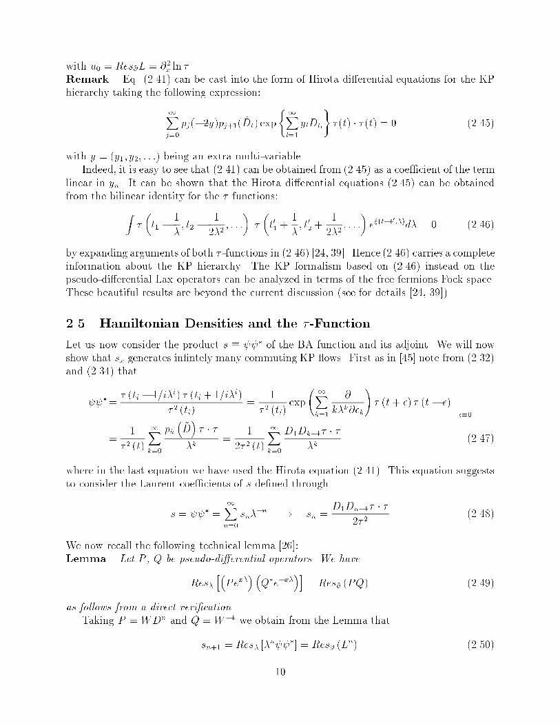
2.5 Hamiltonian Densities and the � -Function
Let us now consider the product s � � of the BA function and its adjoint. We will nowshow that sx generates in�ntely many commuting KP ows. First as in [45] note from (2.32)and (2.34) that
�=� (ti � 1=i�i) � (ti + 1=i�i)
� 2 (ti)=
1
� 2 (ti)exp
1Xk=1
@
k�k@�k
!� (t+ �) � (t� �)
������=0
=1
� 2 (t)
1Xk=0
pk�~D�� � �
�k=
1
2� 2 (t)
1Xk=0
D1Dk�1� � �
�k(2.47)
where in the last equation we have used the Hirota equation (2.41). This equation suggeststo consider the Laurent coe�cients of s de�ned through
s = � =1Xn=0
sn��n ! sn =
D1Dn�1� � �
2� 2(2.48)
We now recall the following technical lemma [26]:Lemma. Let P , Q be pseudo-di�erential operators. We have
Res�h�Pex�
� �Q�e�x�
�i= Res@ (PQ) (2.49)
as follows from a direct veri�cation.
Taking P = WDn and Q = W�1 we obtain from the Lemma that
sn+1 = Res� [�n �] = Res@ (L
n) (2.50)
10

From (2.47) we �nd
sn = Res@�Ln�1
�=
1
2� 2 (t)D1Dn�1� � � = @x@n�1 ln � (2.51)
Since u0 = @2 ln � we can rewrite @xsn as
@xsn =@u0
@tn�1(2.52)
Note that in notation of the previous subsections the above equation shows that the conserved
densities of the KP hierarchy �(m)1 are equal to Hamiltonian densitiesHm � Res@ (L
m) of the
KP hierarchy, which generate commuting ows through relation @xHn = (@=@tn)u0. Accord-
ingly the KP hierarchy has an in�nite set of commuting symmetries associated with in�nite
set of the conserved Hamiltonians. This translates into commutativity of Hamiltonians on
the level of the Poisson brackets indicating integrability of the system. These symmetries arecalled isospectral symmetries as they preserve the spectrum of the underlying linear problem.
11

3 Symmetry Reduction of the Integrable Systems. Five
Constructions of the CKP models.
3.1 Symmetry of Nonlinear Evolution Equation
We will discuss notion of symmetry of partial di�erential equatiom on the basis of an evolu-
tion equation:@u
@t= K[u(t)] (3.1)
with some nonlinear operator K. An evolution equation @u@�
= G[u(t)] is called a symmetry
of (3.1) if the Fr�echet derivative of K at the point u in the direction of G
K 0[u(t)] (G) �@
@�K[x; u(t) + �G; u0 + �Gx; : : :]j�=0 (3.2)
Gx �@G
@x+Xk�1
@G
@u(k)u(k+1) (3.3)
satis�es
K 0[u(t)] (G) �@G
@t+G0[u(t)] (K) (3.4)
Hence a condition that G is a symmetry of (3.1) is equivalent to having v � G[u(t)] satisfythe linearized version of (3.1) with a background u(t) i.e. dv=dt = K 0[u(t)] (v). In otherwords u+�v satis�es (3.1) for all solutions u of (3.1) for an arbitrarily small �. Therefore thelinearized version of the nonlinear evolution equation contains all the pertinent informationabout its symmetries.
We can also rephrase condition (3.4) as commutativity [Dt ; D� ] = 0 of two di�erentia-tions associated with t and �
Dt �@
@t+K
@
@u+Kx
@
@ux+ : : : (3.5)
D� �@
@�+G
@
@u+Gx
@
@ux+ : : : (3.6)
Examples:Consider the KdV equation: ut = 6uu0 � u000 in terms of !0 = u:
!t = K[!] = 6!0 2 � !000 (3.7)
Condition (3.4) gives
dv=dt = K 0[!(t)] (v) = 3!0v0 �1
2v000 (3.8)
Consider Galilean symmetry of KdV:
! ! ~! = !(x+ 3t�) +1
2x� (3.9)
12

which can be cast in the form of \evolution" equation:
v = G =d~!
d�j�=0 = 3t!0 +
1
2x (3.10)
Taking into account that vx = 3t!00+ 12, vxxx = 3t!IV and also dv=dt = 3!0+3t (3!0 2 � !000)
0
we can verify that the Galilean transformation is a \non-isospectral" symmetry of the KdV
equation.
For the KP eq. (2.44) its linearized version takes the form:
dv=dt =1
4
@3v
@x3+ 3
@(u0v)
@x+3
4@�1
@2v
@t22(3.11)
3.2 Symmetry Reduction and the CKP Hierarchy
We will �rst show that the quantity @x(�) is a symmetry of the KP equation with � and are (adjoint ) eigenfunctions of L i.e. they satisfy (2.5) and (2.36):
@
@tm� = Lm+� ;
@
@tm = �Lm�
+ (3.12)
where Lm� is the adjoint operator of Lm.Let us particularly stress that the above eigenfunctions do not need to be Baker-Akhiezer
eigenfunctions of L and @x(�) in general di�ers from quantity sx � @x �, which, as
we have seen in the previous section, generates an in�nite set of commuting symmetriesassociated with in�nite set of the conserved Hamiltonians of the KP hierarchy.
For n = 2 equation (3.12) gives:
@�
@t2=@2�
@x2+ 2u0� ;
@
@t2= �
@2
@x2� 2u0 (3.13)
while for n = 3 we obtain from (3.12):
@�
@t3=@3�
@x3+ 3u0
@�
@x+3
2u00� +
3
2
@�1x
@u0
@t2
!�
@
@t3=@3
@x3+ 3u0
@
@x+3
2u00�
3
2
@�1x
@u0
@t2
! (3.14)
Using equations (3.13) and (3.14) one can show as in [45, 18] that S � � satis�es the
evolution equation@S
@t3=
1
4
@3S
@x3+ 3u0
@S
@x+3
4@�1
@2Sx
@t22(3.15)
and therefore the quantity Sx � @xS satis�es a linearized version of the KP equation (3.11).Hence according to the above de�nition Sx is a symmetry of the KP equation.
Recall now that in components the Lax equation (2.1) takes the following form of partial
di�erential equations
@run = Fn;r (u0; u1; : : : ; ur+n�1) n = 0; : : : (3.16)
13
with di�erential polynomials Fn;r in u0; u1; : : : ; ur+n�1. In particular we have a hierarchy of
ow equations:
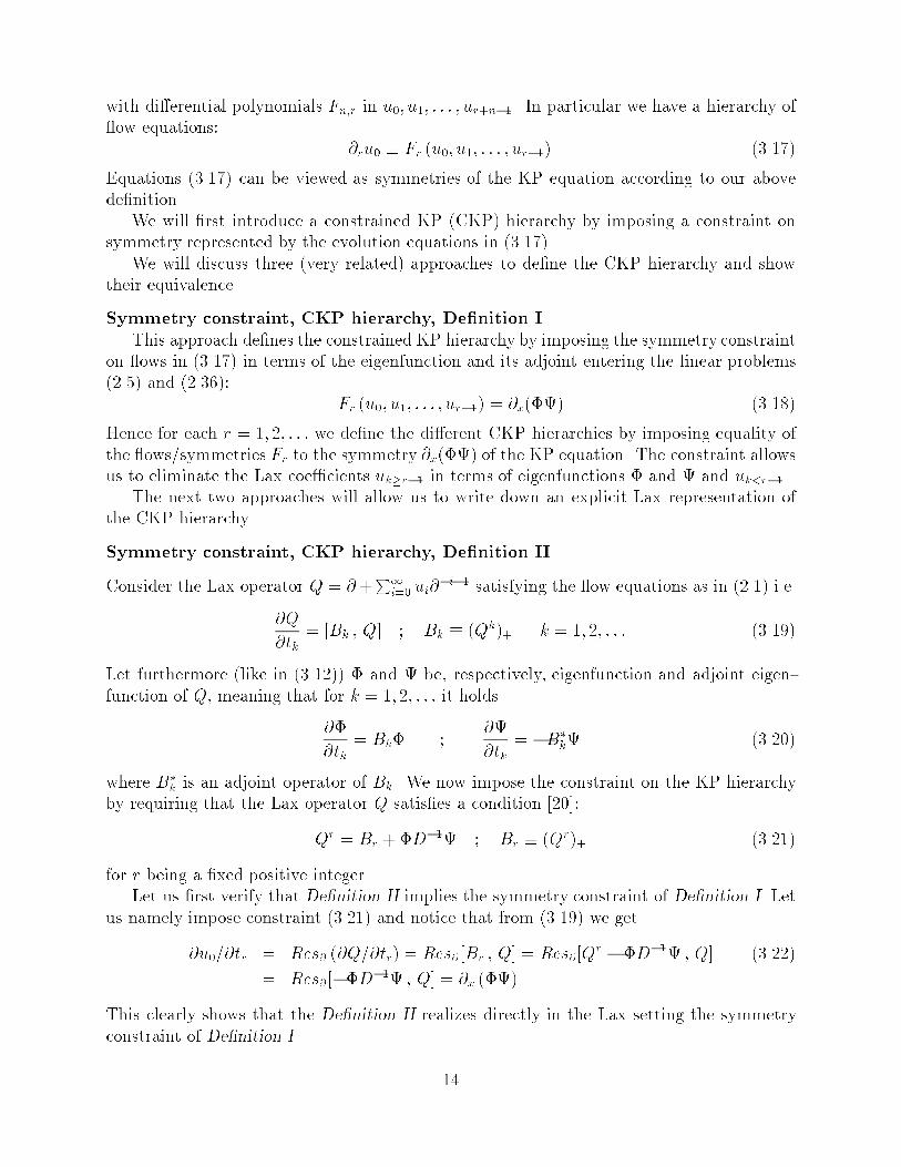
@ru0 � Fr (u0; u1; : : : ; ur�1) (3.17)
Equations (3.17) can be viewed as symmetries of the KP equation according to our above
de�nition.
We will �rst introduce a constrained KP (CKP) hierarchy by imposing a constraint on
symmetry represented by the evolution equations in (3.17).
We will discuss three (very related) approaches to de�ne the CKP hierarchy and show
their equivalence.
Symmetry constraint, CKP hierarchy, De�nition I
This approach de�nes the constrained KP hierarchy by imposing the symmetry constraint
on ows in (3.17) in terms of the eigenfunction and its adjoint entering the linear problems
(2.5) and (2.36):
Fr (u0; u1; : : : ; ur�1) = @x(�) (3.18)
Hence for each r = 1; 2; : : : we de�ne the di�erent CKP hierarchies by imposing equality ofthe ows/symmetries Fr to the symmetry @x(�) of the KP equation. The constraint allowsus to eliminate the Lax coe�cients uk�r�1 in terms of eigenfunctions � and and uk<r�1.
The next two approaches will allow us to write down an explicit Lax representation ofthe CKP hierarchy.
Symmetry constraint, CKP hierarchy, De�nition II
Consider the Lax operator Q = @+P1i=0 ui@
�i�1 satisfying the ow equations as in (2.1) i.e.
@Q
@tk= [Bk ; Q] ; Bk � (Qk)+ k = 1; 2; : : : (3.19)
Let furthermore (like in (3.12)) � and be, respectively, eigenfunction and adjoint eigen-
function of Q, meaning that for k = 1; 2; : : : it holds
@�
@tk= Bk� ;
@
@tk= �B�
k (3.20)
where B�k is an adjoint operator of Bk. We now impose the constraint on the KP hierarchy
by requiring that the Lax operator Q satis�es a condition [20]:
Qr = Br + �D�1 ; Br � (Qr)+ (3.21)
for r being a �xed positive integer.
Let us �rst verify that De�nition II implies the symmetry constraint of De�nition I. Let
us namely impose constraint (3.21) and notice that from (3.19) we get
@u0=@tr = Res@ (@Q=@tr) = Res@[Br ; Q] = Res@[Qr ��D�1 ; Q] (3.22)
= Res@[��D�1 ; Q] = @x (�)
This clearly shows that the De�nition II realizes directly in the Lax setting the symmetry
constraint of De�nition I.
14

Lemma. The time evolution of the pseudo-di�erential operator �D�1 is qiven by:
@
@tk�D�1 = [Bk ; �D
�1]� (3.23)
The proof is a consequence of following technical observations based on (3.20):
�Bk�D
�1��= (Bk�)0D
�1 =@�
@tkD�1 (3.24)
and
���D�1Bk
��= ��D�1 (B�
k)0 = �D�1 @
@tk(3.25)
What we learn from the above lemma is that if we de�ne the Lax operator L such
that its purely pseudo-di�erential part is L� = �D�1 then L� satis�es automatically the
KP ow equations: @L�=@tk = [Bk ; L]�. Note that in the last equation we used that[Bk ; L]� = [Bk ; L�]�. These observations lead us to the next de�nition of CKP hierarchy.
Symmetry constraint, CKP hierarchy, De�nition III
Here we work with Lax operator of the CKP hierarchy de�ned as
L = Dr +r�2Xl=0
UlDl + �D�1 (3.26)
@L
@tk= [
�Lk=r
�+; L] (3.27)
We �rst address an issue of equivalence between De�nition II and De�nition III, which iseasy to establish when making a connection Qr � L. It is then easy to see that the two owsgiven below are equivalent (Bk =
�Qk�+=�Lk=r
�+):
@Q=@tk =��Qk�+; Q
�$ @L=@tk =
��Qk�+; L
�=��Lk=r
�+; L
�(3.28)
We have already seen in (3.23) that the pseudo-di�erential part of L from (3.26) evolves
according to the Sato's formalism. Let us now investigate evolution of the di�erential partBr = (Qr)+ = (L)+ of L:
@Br=@tk = [Bk ; L]+ = [Bk ; Br] + [Bk ; �D�1]+ (3.29)
which after using Zakharov-Shabat equation (2.3) becomes:
@Bk=@tr = [Bk ; �D�1]+ (3.30)
valid for all k = 1; 2; : : : . Equation (3.30) describes how the CKP constraint condition is
being imposed on the ows of KP coe�cients in Bk. Let us study consequences of (3.30) insome simple cases. The �rst nontrivial case occurs for k = 2 with B2 = (Q2)+ = D2+2u0 =
D2 + U0. From (3.30) it follows:
2@u0=@tr = [D2 ; �D�1]+ = 2@x(�) (3.31)
15

which reproduces the ow equation being basis for the De�nition I of the CKP hierarchy,
establishing henceforth equivalence between De�nition I and De�nition III.
For k = 3 we have B3 = (Q3)+ = D3 + 3u0D + 3u1 + 3@xu0 = D3 + U0D + U1. From
(3.30) it follows this time that:
@(3u0D + 3u1 + 3u00)=@tr = [D3 ; �D�1]+ = 3�00+ 3�00 + 3 (�)0D (3.32)
or
@u1=@tr = � (�0)0
(3.33)
Consider the Lax operator L having the form as in (3.26) and satisfying (3.27). One can
ask whether � () are automatically the (adjoint) eigenfunctions. The following Lemma
answers this question a�rmatively.
Lemma. Let L = L++�D�1, with r being the order of L+. Then the Lax equations
of motion @@tkL = [Bk ; L ] imply:
" @
@tk� � (Bk�)0
!D�1+ �D�1
@
@tk+ (B�
k)0
!#= 0 (3.34)
where Bk = (Lk=r)+ ; B�k = (Lk=r)�+
Remark. Eq. (3.34) is equivalent to the in�nite set of equations:" @
@tk�� (Bk�)0
!@lx+ �@lx
@
@tk+ (B�
k)0
!#= 0 ; l = 0; 1; 2; : : : (3.35)
An obvious solution of (3.35) seems to be:
@
@tk�� (Bk�)0 =
@cr
@tk� (3.36)
@
@tk+ (B�
k)0 = �@cr
@tk
where cr is x-independent. Thus, up to a x-independent phase transformation �! ecr� and
! e�cr, which does not change the Lax operator, � () are (adjoint) eigenfunctions.
Examples:
r=1. The simplest case is when r = 1 for which we have:
F1 = @xu0 = @x�! u0 = �+ const (3.37)
Inserting this into (3.13) (with zero integration constant) we get
@�
@t2=@2�
@x2+ 2�2 ;
@
@t2= �
@2
@x2� 2�2 (3.38)
in which we recognize the Nonlinear Schr�odinger (NLS) equations being the �rst (non-trivial) ow of the AKNS hierarchy. Eqs. (3.38) are also results of the Sato equation (2.1) for two-
boson hierarchy [41, 5] de�ned by the Lax operator Q = L = D + �D�1. Expressions for
16
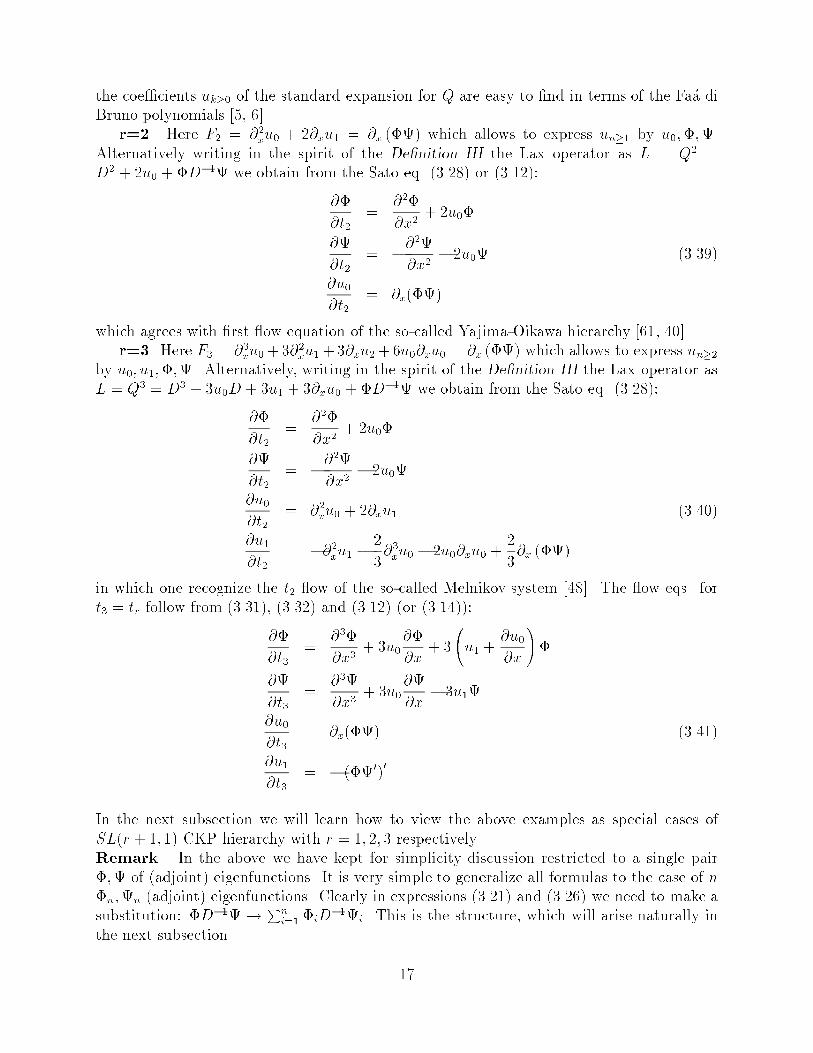
the coe�cients uk�0 of the standard expansion for Q are easy to �nd in terms of the Fa�a di
Bruno polynomials [5, 6].
r=2. Here F2 = @2xu0 + 2@xu1 = @x (�) which allows to express un�1 by u0;�;.
Alternatively writing in the spirit of the De�nition III the Lax operator as L = Q2 =
D2 + 2u0 + �D�1 we obtain from the Sato eq. (3.28) or (3.12):
@�
@t2=
@2�
@x2+ 2u0�
@
@t2= �
@2
@x2� 2u0 (3.39)
@u0
@t2= @x(�)
which agrees with �rst ow equation of the so-called Yajima-Oikawa hierarchy [61, 40]
r=3. Here F3 = @3xu0+3@2xu1+3@xu2+6u0@xu0 = @x (�) which allows to express un�2by u0; u1;�;. Alternatively, writing in the spirit of the De�nition III the Lax operator asL = Q3 = D3 + 3u0D + 3u1 + 3@xu0 + �D�1 we obtain from the Sato eq. (3.28):
@�
@t2=
@2�
@x2+ 2u0�
@
@t2= �
@2
@x2� 2u0
@u0
@t2= @2xu0 + 2@xu1 (3.40)
@u1
@t2= �@2xu1 �
2
3@3xu0 � 2u0@xu0 +
2
3@x (�)
in which one recognize the t2 ow of the so-called Melnikov system [48]. The ow eqs. fort3 = tr follow from (3.31), (3.32) and (3.12) (or (3.14)):
@�
@t3=
@3�
@x3+ 3u0
@�
@x+ 3
u1 +
@u0
@x
!�
@
@t3=
@3
@x3+ 3u0
@
@x� 3u1
@u0
@t3= @x(�) (3.41)
@u1
@t3= � (�0)
0
In the next subsection we will learn how to view the above examples as special cases of
SL(r + 1; 1) CKP hierarchy with r = 1; 2; 3 respectively.Remark. In the above we have kept for simplicity discussion restricted to a single pair
�; of (adjoint) eigenfunctions. It is very simple to generalize all formulas to the case of n�n;n (adjoint) eigenfunctions. Clearly in expressions (3.21) and (3.26) we need to make a
substitution: �D�1 !Pni=1 �iD
�1i. This is the structure, which will arise naturally in
the next subsection.
17
3.3 CKP Hierarchy as SL(m;n)-type Lax Hierarchy and its Bi-
Poisson Structure
Let us introduce a ratio of two di�erential operators (with m = r + n in notation of the
previous subsection).
Lm;n �L(m)
L(n)n � m� 1 (3.42)
where
L(m) = Dm+um�1Dm�1+ : : :+u1D+u0 ; L(n) = Dn+~un�1D
n�1+ : : :+~u1D+~u0 (3.43)
Let f (m)i ; i = 1; : : : ;mg and f
(n)i ; i = 1; : : : ; ng be a basis for the kernels of L(m) and
L(n), respectively, i.e. we have L(�) (�)i = 0 ; i = 1; : : : ; � = m or n. Alternatively, we can
rewrite (3.43) as
L(m) = (D + vm) (D + vm�1) � � � (D + v1) ; L(n) = (D + ~vn) (D + ~vn�1) � � � (D + ~v1)(3.44)
with
vi = @
0@log Wi�1[
(m)1 ; : : : ;
(m)i�1 ]
Wi[ (m)1 ; : : : ;
(m)i ]
1A ; W0 = 1 (3.45)
and similar expressions for ~vi.Taking the above into consideration we can rewrite (3.42) as [12, 62]
Lm;n =1Y
j=m
(D + vj)nYl=1
(D + ~vl)�1
(3.46)
(see also [16, 25, 53] for discussion of the pseudo-di�erential operators of the constrained KPhierarchy). We will now study the Poisson structures of the hierarchy de�ned by the Lax
operators of the form given in (3.46). It is easy to prove the following Proposition [62, 12].Proposition. The Poisson bracket relation:
fvi ; vjgPB = �ij �0(x� y) i; j = 1; : : :m
f~vr ; ~vsgPB =��rs �0(x� y) r; s = 1; : : : ; n (3.47)
fvi ; ~vlgPB =0
is equivalent to
f hLm;nj Xi ; hLm;nj Y i gPB = TrA�(Lm;nX)+Lm;nY � (XLm;n)+ Y Lm;n
�(3.48)
where the subscript PB stands for the Poisson bracket as de�ned by (3.47).
We now introduce a Dirac constraint:
m;n =mXj=1
vj �nXl=1
~vl = 0 (3.49)
18

which is second-class due to:
fm;n ; m;ngPB = (m� n) �0(x� y) (3.50)
Condition (3.49) expresses tracelessness of the underlying graded SL(m;n) algebra. Cor-
responding Poisson algebra of diagonal part of the graded SL(m;n) Kac-Moody algebra is
obtained by the usual Dirac bracket calculation:
fvi ; vjgDB=
��ij �
1
m� n
��0(x� y) i; j = 1; : : : ;m
f~vr ; ~vsgDB=�
��rs +
1
m� n
��0(x� y) r; s = 1; : : : ; n (3.51)
fvi ; ~vrgDB=1
m� n�0(x� y)
Proposition. The Dirac bracket (3.51) takes the following form in the Lax operator rep-
resentation:
f hLm;nj Xi ; hLm;nj Y i gDB = f hLm;nj Xi ; hLm;nj Y i gPB
+1
m� n
Zdx Res ([Lm;n ; X ]) @�1Res ([Lm;n ; Y ])
The proof follows from evaluation of the extra term of the relevant Dirac bracket:
�
Zf hLm;nj Xi ; m;n gPB fm;n ; m;n g
�1
DBfm;n ; hLm;nj Y i gDB (3.52)
One easily veri�es (3.52) using (3.50):
f hLm;nj Xi ; m;n(z) gPB = �h[ �(x� z) ; Lm;n ]j Xi = �Res ([X ; Lm;n ]) (z) (3.53)
Formula (3.52) contains as special cases n = m� 1 corresponding to the constrained KPhierarchy with L+ = D and n = 0 corresponding to the m-KdV hierarchy (see e.g. [27]).For the intermediary cases 0 < n < m � 1 this formula presents a compact expression for
the bracket structure of the SL(m;n) CKP hierarchy.
The Lax operator from (3.42) restricted to the constrained manifold de�ned by (3.49)can be parametrized as
Lm;n � Lm;n jm;n=0=
n+1Yl=m�1
(D + ecl) 1Yl=n
(D + ecl + ~vl)
D �
m�1Xl=1
ecl!
nYl=1
(D + ~vl)�1 (3.54)
We can alternatively rewrite the expression (3.54) as
Lm;n =nXl=1
eAl
nYi=l
(D + ~vi)�1 +
m�n�2Xl=0
eAl+n+1Dl +Dm�n (3.55)
with the second bracket structure automatically given by the formula (3.52).For the special case m�n = r = 1 we have a canonical representation for variables (vi; ~vl)
with 1 � i � m ; 1 � l � m � 1 in Lm;m�1 =Q1j=m (D + vj)
Qm�1l=1 (D + ~vl)
�1 in terms of
19

the pairs (cr; er)m�1r=1 , which are the \Darboux" canonical pairs for the second KP bracket
satisfying fci(x) ; el(y)g = ��il@x�(x � y) for i; l = 1; 2; : : : ;m � 1. The representation is
[12]:
~vl = �el �m�1Xp=l
cp l = 1; 2; : : : ;m� 1 (3.56)
vi = �ei�1 �m�1Xp=i
cp = �ci + ~vi i = 1; : : : ;m (3.57)
Eq. (3.57) includes the special cases of v1 = �Pm�1p=1 cp and vm = �e1. One checks easily
that in this representation the Poisson algebra of ~vl; vi takes indeed the form of the bracket
algebra of graded SL(m;m� 1) Kac-Moody algebra in a diagonal gauge:
fvi ; vjg=(�ij � 1) �0(x� y) i; j = 1; : : : ;m
f~vp ; ~vlg=� (�pl + 1) �0(x� y) p; l = 1; : : : ;m� 1 (3.58)
fvi ; ~vlg=��0(x� y)
We can interpret (3.54) as a superdeterminant of the graded SL(m;n) matrix in a diago-nal gauge, which for KdV case n = 0 becomes an ordinary determinant as in Fateev-Lukyanov[29] expression:
Lm;0 =mYi=1
(D + vi) = Dm + eAm�1Dm�2 + : : :+ eA1 ;
mXi=1
vi = 0 (3.59)
Example. As an example let us take m = 2; n = 1 in (3.54). Then:
L2;1 = (D + c1 + ~v1) (D � c1) (D + ~v1)�1 = � [(~v1 + c1)
0 + c1(~v1 + c1)] (D + ~v1)�1 +D
(3.60)as follows by direct calculation making use of an obvious identity (D + c) (D + v)�1 =(c� v) (D + v)�1 + 1.
One notices the absence of the term proportional toDm�n�1 in (3.55) due to the SL(m;n)trace zero condition. Another feature is the presence of the constant term An+1 in the Laxoperator Lm;n (for m�n > 1). This fact enables us to prove that SL(m;n)-CKP hierarchy is
a bi-Poisson hierarchy. Consider namely L0m;n = Lm;n�� obtained by rede�ning the D0 = 1term in the Lax operator by addition of the constant �. Clearly the value of the of bracket(3.52) for the new Lax is
n DL0m;n
��� Xi ; DL0m;n��� Y i oDB= TrA
��L0m;nX
�+L0m;nY �
�XL0m;n
�+Y L0m;n
�
+1
m� n
ZdxRes
�hL0m;n ; X
i�@�1Res
�hL0m;n ; Y
i�� �
DL0m;n j [X; Y ]R
E(3.61)
where we introduced an R-commutator [X; Y ]R � [X+; Y+]�[X�; Y�] with subscripts � de-noting projection on pure di�erential and pseudo-di�erential parts of the pseudo-di�erential
operators X;Y . De�ne next an R-bracket f�; �gR1 as a bracket obtained by substituting
R-commutator [X; Y ]R for the ordinary commutator [54, 58, 10]:
f hLj Xi ; hLj Y i gR
1 � �hL j [X; Y ]Ri (3.62)
20
Relation (3.61) shows that f�; �gDB + �f�; �gR1 satis�es the Jacobi identity. We can state this
result as:
Proposition. SL(m;n)-CKP hierarchy is bi-Poisson with brackets f�; �gDB and f�; �gR1de�ning a compatible pair of brackets.
This Proposition establishes the fundamental criterion for integrability of the SL(m;n)-
CKP hierarchy. Clearly the argument holds also for the case m�n = 1, where one adds the
constant � to zero representing the missing constant term.
Let us now concentrate on the pseudo-di�erential part of Lm;n from (3.55). We can
rewrite it as
(Lm;n)� =nXl=1
rl
nYi=l
D�1qi (3.63)
rl = eAle�R~vl ; qn = e
R~vn ; qi = e
R(~vi�~vi+1) ; i = 1; : : : ; n� 1 (3.64)
Let us de�ne the quantity
Ql;i � (�1)i�nZqi
Zqi�1
Z: : :
Zql (dx
0)i�l+1 1 � l � i � n (3.65)
Then using that D�1Q1;i�1qi = D�1Q1;iD �Q1;i we obtain for quantity in eq.(3.63)
(Lm;n)� =nXi=2
r(1)i
nYl=i
D�1ql + r1D�1 (�Q1;n�1qn) (3.66)
where
r(1)i � ri + r1Q1;i�1 i = 2; : : : ; n (3.67)
The above process can be continued to yield an expression
(Lm;n)� =nXi=1
�iD�1i (3.68)
with
�i = ri +i�1Xn=1
rn
i�nXsi�n�1=si�n�2+1
� � �i�nX
s2=s1+1
i�nXs1=1
Qn;i�si�n�1�1Qi�si�n�1;i�si�n�2�1 � � �
� � � Qi�s2;i�s1�1Qi�s1;i�1 1 � i � n (3.69)
n = qn ; i = (�1)n�iqn
Zqn�1
Z: : :
Zqi (dx
0)n�i 1 � i � n� 1 (3.70)
Note that the new variables i coincide with elements (n)i in the kernel of L(n). It follows
from the construction opposite to the one shown above and involving the following relation
(see [13] for more details):
(Lm;n)� =nXi=1
�iD�1i (3.71)
=nXi=1
A(n)i
�D +B
(n)i
��1 �D +B
(n)i+1
��1� � �
�D +B(n)
n
��1(3.72)
21

where the new variables are :
A(n)i = (�1)n�i
iXs=1
�sW [n; : : : ;i+1;s]
W [n; : : : ;i+1](3.73)
B(n)i = @x ln
W [n; : : : ;i+1;i]
W [n; : : : ;i+1](3.74)
From (3.72) we see that ~vi = B(n)i and from (3.74) it follows that
(n)i = i.
Example. For n = 2 relations (3.73)-(3.74) become
A(2)2 = �11 + �22 ; A
(2)1 = ��11
�@x ln
�12 1
�(3.75)
B(2)2 = @x ln2 ; B
(2)1 = @x ln
h1
�@x ln
�12 1
�i(3.76)
Equivalence between (3.72) and (3.71) follows then by inspection.Proposition. �i;i are canonical-Darboux �elds for the �rst bracket of the SL(n + 1; n)CKP hierarchy :
f�i ; j g1 = ��ij�(x� y) ; i; j = 1; : : : ; n (3.77)
3.4 A�ne sl(n + 1) Origin of SL(n + 1; n) CKP Hierarchy.
In this subsection we will establish a connection betweenGeneralized Non-linear SchroedingerGNLS matrix hierarchy for the hermitian symmetric space sl(n+1) [33] and the constrained
KP hierarchy.We �rst introduce ZS-AKNS scheme arising from the linear matrix problem for A 2 G
with G being a Lie algebra [32, 49]:
@=A ; @ =@
@t1= @x (3.78)
@tm=Bm m = 2; 3; : : : (3.79)
The compatibility condition for the linear problem (3.78) and (3.79) leads to the Zakharov-
Shabat (Z-S) integrability equations
@mA� @Bm + [A ; Bm] = 0 ; @m � @tm (3.80)
Let us use the following decomposition in (3.78):
A = �E +A0 with E =2�a �H
�2a(3.81)
where �a is a fundamental weight and �a are simple roots of G. The element E is used todecompose the Lie algebra G as follows:
G = Ker(adE)� Im(adE) (3.82)
22
where theKer(adE) has the formK0�u(1) and is spanned by the Cartan subalgebra of G and
step operators associated to roots not containing �a. Moreover Im(adE) is the orthogonal
complement of Ker(adE).
From now on we consider G = sl(n + 1) with roots � = �i + �i+1 + : : : + �j for some
i; j = 1; : : : ; n , E = 2�n:H�2n
, �n is the nth fundamental weight and Ha, a = 1; : : : ; n are the
generators of the Cartan subalgebra. This decomposition generates the symmetric space
sl(n+ 1)=sl(n)� u(1) (see [9] for details).
ZS-AKNS scheme becomes in this case the GNLSn (=sl(n + 1) GNLS) hierarchy. In
matrix notation we have:
E =1
n+ 1
0BBBBBBB@
1
1
1. . .
�n
1CCCCCCCA
(3.83)
The model is de�ned by A0 2 Ker(adE) and is parametrized by �elds qa and ra, a = 1; : : : ; naccording to:
A0 =nXa=1
�qaE(�a+:::+�n) + raE�(�a+:::+�n)
�(3.84)
which in the matrix form can be rewritten as
A0 =
0BBBBBBB@
0 � � � 0 � � � q10 0 � � � 0 q2
0. . .
......
. . . qnr1 r2 � � � rn 0
1CCCCCCCA
(3.85)
It can be shown that the ows as de�ned in (3.78) and (3.81) satisfy the recurrence relation:
@mA0 = R@m�1A
0 ; R ��@ � adA0 @�1adA0
�adE (3.86)
where we have de�ned a recursion operator R [33, 9].
The connection to the CKP hierarchy is �rst established between linear systems de�ningboth hierarchies. With (3.83) and (3.85) the linear problem from (3.78) is explicitly given
by:0BBBBBBB@
@ � �=(n+ 1) 0 � � � 0 q10 @ � �=(n + 1) 0 � � � q2...
. . ....
0 @ � �=(n + 1) qnr1 r2 � � � rn @ + n�=(n + 1)
1CCCCCCCA
0BBBBBBB@
1 2...
n n+1
1CCCCCCCA= 0
(3.87)Perform now the phase transformation:
k �! � k = exp
��
1
n+ 1
Z� dx
� k k = 1; : : : ; n+ 1 (3.88)
23

We now see that thanks to the special form of E in A = �E +A0, (3.87) takes a simple and
equivalent form: 0BBBBBBB@
@ 0 � � � 0 q10 @ 0 � � � q2...
. . ....
0 @ qnr1 r2 � � � rn @ + �
1CCCCCCCA
0BBBBBBB@
� 1� 2...� n� n+1
1CCCCCCCA= 0 (3.89)
The linear problem (3.89) after elimination of � k ; k = 1; : : : ; n takes a form of the scalar
eigenvalue problem:
� [@ �nXk=1
rk@�1qk] � n+1 = � � n+1 (3.90)
in terms of a single eigenfunction � n+1 and the pseudo-di�erential operator
Ln = @ �nXk=1
rk@�1qk (3.91)
This formally relates GNLSn hierarchy to the SL(n + 1; n) CKP hierarchy on basis of cor-respondence of the linear problems characterizing them. To fully establish their completeequivalence one can show that both models possess the same recurrence operators and there-fore all the ows are identical see [9] ([20] describes the the case n = 1). We �rst note thatthe successive ows (3.86) related by the recursion operator (3.86) are given by
@n
riql
!= R(i;l);(j;m)
rjqm
!= (3.92)
(�@ + rk@
�1qk) �ij + ri@�1qj ri@
�1rm + rm@�1ri
�ql@�1qj � qj@
�1ql (@ � qk@�1rk) �lm � ql@
�1rm
!@n�1
rjqm
!
From relation between the recursion matrix and two �rst bracket structure R = P2P�11 and
(3.92) one �nds an explicit expression for the second bracket [9] to be :
P2 =
ri@
�1rj + rj@�1ri (@ �
Pk rk@
�1qk) �im � ri@�1qm
(@ �Pk qk@
�1rk) �lj � ql@�1rj ql@
�1qm + qm@�1ql
!(3.93)
in the same basis as in (3.92).
The following Proposition proves the equivalence between sl(n + 1) GNLS hierarchyde�ned and the SL(n+ 1; n) CKP hierarchy introduced in the previous subsection.Proposition. Flows
@tmLn = [(Lmn )+ ; Ln] (3.94)
@tmri =
@ �
nXk=1
rk@�1qk
!m!+
ri (3.95)
@tmqi = �
�@ +
nXk=1
qk@�1rk
!m!+
qi (3.96)
24

of SL(n + 1; n) CKP hierarchy containing the Lax operator from (3.91) coincide with the
ows produced by the recursion operator R (3.92) of the sl(n+ 1) GNLS hierarchy
Proof is given in [9] and is accomplished by showing that both hierarchies have identical
recursion operators. Especially (3.96) yields for m = 2:
@qi
@t2= �@2xqi + 2qi
nXb=1
qb rb
@ri
@t2= @2xri � 2ri
nXb=1
qb rb (3.97)
for a = 1; : : : ; n. These are the GNLS equations [33], which have been derived in [9] entirely
from the AKS formalism [1] (see also [36]) associated with an a�ne Lie algebraic structure
(loop algebra G � G C[�; ��1] with G = sl(n+ 1)). This construction reveals an a�ne Lie
algebraic structure underlying the integrability of the SL(n+ 1; n) CKP hierarchy.
25
4 Darboux-B�acklund Techniques of SL(p; q) CKP Hier-
archies and Constrained Generalized Toda Lattices
4.1 Emergence of the Toda structure from Two-Bose KP System
The two-boson KP system de�ned by the Lax operator L = D+�D�1 � D+ a (D � b)�1
is the most basic constrained KP structure. It belongs to the SL(2; 1) CKP system.
We start with the initial \free" Lax operator L(0) = D and perform a following transfor-
mation:
L(1) =��(0)D�(0)�1
�D��(0)D�1�(0)�1
�= D +
��(0)
�ln�(0)
�00�D�1
��(0)
��1(4.1)
which we call a DB transformation. The construction below is a special application of
properties listed in Appendix B including eq. (B.9).
Successive application of DB transformations leads to the following recursive expressions:
L(k+1)=��(k)D�(k)�1
�L(k)
��(k)D�1�(k)�1
�= D + �(k+1)D�1(k+1) (4.2)
�(k+1)=�(k)�ln�(k)
�00+��(k)
�2(k) ; (k+1) =
��(k)
��1(4.3)
Introduce now�k = ln�(k) ! �(k) = e�k k = 0; : : : (4.4)
which allows us to rewrite (4.3) as a (ordinary one-dimensional) Toda lattice equation:
@2�k = e�k+1��k � e�k��k�1 (4.5)
Related objects n are:�n = n+1 � n (4.6)
which satisfy due to eq. (4.5) the follwoing form of the Toda lattice equation:
@2 n = e n+1+ n�1�2 n (4.7)
with n = 0 for n � 0. Comparing (4.7) with Jacobi's theorem (B.7) we �nd the Wronskian
representation for n:
n = lnWn[�; @�; : : : ; @n�1�] with � = �(0) (4.8)
Correspondingly �(k) acquires the form:
�(k) =Wk+1[�; @�; : : : ; @
k�]
Wk[�; @�; : : : ; @k�1�](4.9)
We recognize at the right hand side of (4.7) a structure of the Cartan matrix for An. Leznov
considered such an equation with Wronskian solution (in two dimensions) in [42].
Hence, the solutions of the (ordinary one-dimensional) Toda lattice equations, withboundary conditions n = 0 for n � 0, reproduce the DB solutions of the ordinary two-
boson KP hierarchy (4.9) upon taking into account that � = �(0) = exp (�0) = exp ( 1).
26

Note that we can write Wn = �n with the � -function �n satisfying Hirota's bilinear
equation for the Toda lattice:
�n@2�n � (@�n)
2= �n+1�n�1 (4.10)
on basis of (B.8).
We will now �nd a linear discrete system (Toda spectral problem), which leads to the
above structure. First de�ne:
Rn =�(n+1)
�(n)=�n+1�n�1
� 2n(4.11)
Sn = @�ln�(n+1)
�= @
�ln�n+1
�n
�(4.12)
As result of (4.10) and their de�nition Sn; Rn satisfy the Toda equations of motion:
@ Sn = Rn+1 �Rn (4.13)
@ Rn = Rn (Sn � Sn�1) (4.14)
These equations can also be obtained as a consistency of the spectral system
@n=n+1 + Snn (4.15)
�n =n+1 + Snn +Rnn�1 (4.16)
which de�nes a so-called Toda chain system.
As we will show this purely discrete system contains information about the underlyingcontinuous structure. This structure is being revealed when we realize that the lattice jumpn! n + 1 can be given a meaning of the DB transformation. We start by rewriting (4.15)as follows:
@n = n+1 + Snn � n+1 = eRSn@ e�
RSnn (4.17)
or taking into account (4.14) as
n+1 = RneRSn�1@
�Rne
RSn�1
��1n = �(n)@��1(n)n = T (n)n (4.18)
where �(n) = RneRSn�1 and T (n) = �(n)@��1(n) plays a role of the DB transformation
operator generating the lattice translation n! n + 1.The remaining of the Toda spectral equation (4.16) can be given a form (with (n) �
e�RSn�1):
�n =�@ +Rn (@ � Sn�1)
�1�n =
h@ +Rne
RSn�1@�1e�
RSn�1
in
=h@ + �(n)@�1(n)
in = L(n)n (4.19)
of the Lax eigenvalue problem of the two-bose KP Lax system with generic two-bose KPLax operator L = D + �D�1. Hence the Toda lattice spectral problem has been shown
equivalent to the continuous CKP system possessing the symmetry with respect to the DB
transformations.
27

4.2 On the DB Transformations of the SL(r + n; n) CKP Lax Op-
erators
We shall here consider behavior of the general class of constrained KP Lax operators from
SL(r + n; n) CKP hierarchy under an arbitrary DB transformation eL = �D��1L�D�1��1
where � is an eigenfunction of the Lax operator L as given in (3.26). The transformed Lax
operator reads:
eL = �D��1 L+ +
nXi=1
�iD�1i
!�D�1��1 � eL+ + eL� (4.20)
eL+ = L+ + �
�@x���1L+�
��1D�1
���1 (4.21)
eL� = e�0D�1 e0 +
nXi=1
e�iD�1 ei (4.22)
e�0 = �
"@x���1L+�
�+
nXi=1
�@x���1�i
�@�1x (i�) + �ii
�#���D��1L
�� (4.23)
e0 = ��1 ; e�i = �@x���1�i
�; ei = ��
�1@�1x (i�) (4.24)
From the above discussion we know that all involved functions are (adjoint) eigenfunctionsof L (3.26), i.e., they satisfy:
@
@tkf = L
k
r
+f f = �;�i ;@
@tki = �L
�k
r
+i (4.25)
We are interested in the special case when � coincides with one of the original eigenfunctionsof L, e.g. � = �1. Then e�1 = 0 and the DB transformation (4.20) preserves the form (3.26)of the Lax operators involved, i.e., it becomes an auto-B�acklund transformation. Applying
the successive DB transformations in this case yields:
L(k)=T (k�1)L(k�1)�T (k�1)
��1=�L(k)
�++
nXi=1
�(k)i D�1
(k)i ; T (k) � �
(k)1 D
��(k)1
��1(4.26)
�(k+1)1 =
�T (k)L(k)
��(k)1 ;
(k+1)1 =
��(k)1
��1; k = 0; 1; : : : (4.27)
�(k+1)i =T (k)�
(k)i � �
(k)1 @x
���(k)1
��1�(k)i
�(4.28)
(k+1)i =�
��(k)1
��1@�1x
�(k)i �
(k)1
�; i = 2; : : : ; n (4.29)
Using the �rst identity from (4.26), i.e., L(k+1)T (k) = T (k)L(k) , one can rewrite (4.27) in theform:
�(k)1 = T (k�1)T (k�2) � � �T (0)
��L(0)
�k�(0)1
�(4.30)
whereas:
�(k)i = T (k�1)T (k�2) � � � T (0)�
(0)i ; i = 2; : : : ; n (4.31)
28

Finally, for the coe�cient of the next-to-leading di�erential term in (3.26) ur�2 = r ResL1r =
r @2x ln � , we easily obtain from (4.21) (with � = �1) its k-step DB-transformed expression:
1
r
�u(k)r�2 � u
(0)r�2
�= @2x ln
� (k)
� (0)= @2x ln
��(k�1)1 � � ��
(0)1
�(4.32)
Remark. Let us particularly stress that the eigenfunctions we are working with are not
Baker-Akhiezer eigenfunctions of L from (3.26). Imagine, namely that we started with
L = L+ + D�1 �, where ; � are BA functions. Choosing � = would result according
to (4.23) and (4.24) in eL = D. Hence in such case we would be able to transform away the
pseudo-di�erential part of the CKP Lax operator by a �nite number of DB transformations.
4.3 DB Transformation and Eigenfunctions of the Lax Operator
After seeing DB transformation in action in the simple cases shown in the �rst two subsections
of this chapter we are now ready to review the basic properties of DB transformation fromthe point of view of preserving the form of the Lax evolution equation. Related material canbe found in e.g. [19, 51].Lemma. For arbitrary pseudo-di�erential operator A we have the following identity [52]:�
�D��1A�D�1��1�+= �D��1 (A)+ �D
�1��1 � �@x���1((A)+�)
�D�1��1 (4.33)
For L satisfying a general KP-KdV Lax equation @kL =�L
k
r
+ ; L
�the transformed Lax
operator ~L � TLT�1 will satisfy:
@k ~L =�TL
k
r
+T�1 + (@kT )T
�1 ; ~L�
(4.34)
Let � be an eigenfunction of L i.e. Lk
r
+� = @k�, which enters the DB transformation through
T = �D��1. One veri�es easily that for A = Lk
r and � = � equation (4.33) becomes�TL
k
r T�1�+= TL
k
r
+T�1 + (@kT )T
�1 (4.35)
Correspondingly (4.34) takes the form:
@k ~L =
�~L
k
r
+ ; ~L
�(4.36)
and we have therefore established:
Proposition. The DB transformation with an eigenfunction � preserves the form of the
Lax equation (2.1) i.e. the DB transformed Lax operator satis�es the same evolution equation
as the original Lax operator.For the pseudo-di�erential operator A = D + a1D
�1 + : : : we have
Res��D��1A�D�1��1
�= (ln�)00 +Res (A) (4.37)
For the case of the Lax operator L with the � -function satisfying ResL = @2 ln � we get
therefeore [19]:Proposition. Under the DB transformation with an eigenfunction � the � -function asso-
ciated to the Lax operator L transforms according to � ! e� = �� .
29

4.4 Exact Solutions of SL(p; q) CKP hierarchy via DB Transfor-
mations
Armed with the Wronskian identities from Appendix B, we can represent the k-step DB
transformation (4.30)|(4.32) in terms of Wronskian determinants involving the coe�cient
functions of the \initial" Lax operator
L(0) = Dr +r�2Xl=0
u(0)l Dl +
nXi=1
�(0)i D�1
(0)i (4.38)
only. Indeed, using identity (B.9) and de�ning:�L(0)
�k�(0)1 � �(k) k = 1; 2; : : : (4.39)
we arrive at the following general result:
Proposition. The k-step DB-transformed eigenfunctions and the tau-function (4.30)|
(4.32) of the SL(r + n; n) CKP system (3.71) for arbitrary initial L(0) (4.38) are given
by:
�(k)1 =
Wk+1[�(0)1 ; �(1); : : : ; �(k)]
Wk[�(0)1 ; �(1); : : : ; �(k�1)]
(4.40)
�(k)j =
Wk+1[�(0)1 ; �(1); : : : ; �(k�1);�
(0)j ]
Wk[�(0)1 ; �(1); : : : ; �(k�1)]
; j = 2; : : : ; n (4.41)
� (k) = Wk[�(0)1 ; �(1); : : : ; �(k�1)]� (0) (4.42)
where � (0); � (k) are the � -functions of L(0); L(k) , respectively, and �(i) is given by (4.39).
Example Consider SL(2; 1) CKP hierarchy with the Lax operator: L0 = D + �0D�10,
which serves as a starting point of the successive DB transformations:
L(k) = D + �(k)D�1(k) = T (k)L(k)�T (k)
��1(4.43)
�(k) = T (k�1)L(k�1)�(k�1) (4.44)
By iteration we �nd:
�(k)=T (k�1) � � �T (1)T (0)�(L(0))k�(0)
�=Wk+1[�
(0); �(1); : : : ; �(k)]
Wk[�(0); �(1); : : : ; �(k�1)](4.45)
(k)=��(k�1)
��1(4.46)
Comparing two alternative expressions involving the tau-function � (k):
� (k) = �(k) � � ��(1)�(0)� (0) = Wk+1[�(0)1 ; �(1); : : : ; �(k)]� (0) (4.47)
and ResL(k) = �(k)(k) = @2 ln � (k) we arrive at:
@2 lnWk[�(0); �(1); : : : ; �(k�1)] �
Wk+1[�(0); �(1); : : : ; �(k)]Wk�1[�
(0); �(1); : : : ; �(k�2)]
W 2k [�
(0); �(1); : : : ; �(k�1)]
= ��(0)(0) (4.48)
30

which generalizes the structure of the Hirota equation (4.10) found for the case �(0) = (0) =
0 in subsection 3.1.
Example: Construction of the SL(3; 1) CKP Lax operator, i.e., r = 2; n = 1 in (3.26) i.e.
L = D2 + u+A (D �B)�1
= D2 + u+ �D�1 (4.49)
starting from the \free" L(0) = D2. This example is pertinent to the simplest nontrivial
string two-matrix model [11].
From the basic formulas for successive DB transformations (4.27){(4.26), applied to
(4.49), we have:
L(k) = D2 + u(k) + �(k)D�1(k) (4.50)
L(k) ! L(k+1) = T (k)L(k)�T (k)
��1; T (k) = �(k)D
��(k)
��1(4.51)
u(k) = 2ResL12 � 2@2x ln �
(k) = 2@2x ln��(k�1) � � ��(0)
�(4.52)
�(k) � A(k)eRB(k)
= �(k�1)
"@x
�1
�(k�1)@2x�
(k�1) + 2@2x ln��(k�2) � � ��(0)
��+�(k�1)
�(k�2)
#(4.53)
(k) � e�RB(k)
=��(k�1)
��1(4.54)
u(0) = 0 ; (0) = 0 ; �(0) =Z�
d�
2�c(�)e�(�;ftg) ; � (�; ftg) � �x+
Xj�2
�jtj (4.55)
where �(0) in (4.55) is an arbitrary eigenfunction of the \free" L(0) = D2 (the contour �in the complex �-plane is chosen such that the generalized Laplace transform of c(�) iswell-de�ned).
As a corollary from the above proposition, we get in the case of (4.50) :
�(k) = T (k�1) � � �T (0)�@2kx �(0)
�=
Wh�(0); @2x�
(0); : : : ; @2kx �(0)i
Wh�(0); @2x�
(0); : : : ; @2(k�1)x �(0)
i (4.56)
� (k) = Wh�(0); @2x�
(0); : : : ; @2(k�1)x �(0)i
(4.57)
Substituting (4.56),(4.57) into (4.52){(4.54) we obtain the following explicit solutions for
the coe�cient functions of (4.49) :
u(n) = 2@2x lnWh�(0); @2x�
(0); : : : ; @2(n�1)x �(0)i
(4.58)
B(n) = @x ln
0@W
h�(0); @2x�
(0); : : : ; @2(n�1)x �(0)i
Wh�(0); @2x�
(0); : : : ; @2(n�2)x �(0)
i1A (4.59)
A(n) =Wh�(0); @2x�
(0); : : : ; @2nx �(0)iWh�(0); @2x�
(0); : : : ; @2(n�2)x �(0)i
�Wh�(0); @2x�
(0); : : : ; @2(n�1)x �(0)
i�2 (4.60)
In the more general case of SL(r + 1; 1) CKP Lax operator for arbitrary �nite r :
L = Dr +r�2Xl=0
ulDl + �D�1 (4.61)
31
which de�nes the integrable hierarchy corresponding to the general string two-matrix model
(cf. [11, 12]), the generalizations of (4.56) and (4.57) read:
�(k)=T (k�1) � � �T (0)�@k�rx �(0)
�=
Wh�(0); @rx�
(0); : : : ; @k�rx �(0)i
Wh�(0); @rx�
(0); : : : ; @(k�1)�rx �(0)
i (4.62)
1
ru(k)r�2=ResL
1r = @2x ln �
(k) ; � (k) = Wh�(0); @rx�
(0); : : : ; @(k�1)�rx �(0)i
(4.63)
where �(0) is again given explicitly by (4.55).
4.5 Relation to the Constrained Generalized Toda Lattices
Here we shall establish the equivalence between the set of successive DB transformations of
the SL(r + 1; 1) CKP system (4.61) :
L(k+1) = T (k) L(k)�T (k)
��1; T (k) = �(k)D�(k)�1 (4.64)
L(0) = Dr +r�2Xl=0
u(0)l Dl + �(0)D�1(0) (4.65)
and the equations of motion of a constrained generalized Toda lattice system, underlyingthe two-matrix string model, which contains, in particular, the two-dimensional Toda latticeequations.
For simplicity we shall illustrate the above property on the simplest nontrivial case of
SL(3; 1) CKP hierarchy (4.49). We note that eqs.(4.52){(4.54) (or (4.58){(4.60)) can be castin the following recurrence form:
@x lnA(n�1) = B(n) �B(n�1) (4.66)
u(n) � u(n�1) = 2@xB(n) (4.67)
A(n) �A(n�1) = @x
��B(n)
�2+1
2
�u(n) + u(n�1)
��(4.68)
with \initial" conditions (cf. (4.55)) :
A(0) = B(0) = u(0) = 0 ; B(1) � @x ln� (4.69)
where � is so far an arbitrary function. Now, we can view (4.66){(4.68) as a system of lattice
equations for the dynamical variables A(n); B(n); u(n) associated with each lattice site n and
subject to the boundary conditions:
A(n) = B(n) = u(n) = 0 ; n � 0 (4.70)
Taking (4.69) as initial data, one can solve the lattice system (4.66){(4.68) step by step (for
n = 1; 2; : : :) and the solution has precisely the form of (4.58){(4.60).
32

4.6 Darboux-B�acklund Transformation and the Dressing Chain.
As a small digression we will here apply Darboux-B�acklund (DB) transformation to the KdV
hierarchy emphasizing similarity with the approach developed in the KP setting. Recall from
(4.50)-(4.55) that for T = �D��1 we have
T D2T�1 = D2 + 2@2x ln� + ����1�00
�0D�1��1 (4.71)
The inverse scattering problem corresponding to the KdV equation @tu + 3u@u+ 12@3u = 0
is de�ned in terms of the di�erential operator L = D2 + u, which transforms as:
L1 � T�D2 + u
�T�1=D2 + 2@2x ln� + �
���1�00
�0D�1��1
+ u+ �u0D�1��1 (4.72)
In order for L1 to be a di�erential operator we have to demand that the pseudo-di�erentialpart in (4.72) vanishes:
����1�00
�0+ �u0D�1 = 0 (4.73)
which translates into relation between u and �:
u = ��00
�� �0 = �f
20 � f
00 � �0 (4.74)
where �0 is an integration constant and f0 � (ln�)0. In this notation:
L = D2 + u = D2 � f20 � f00 � �0 = (D + f0) (D � f0)� �0 (4.75)
Since T = D � f0 and Ty = �D � f0 we can factorize the Lax operator L according to
L = �T y T + �0 (4.76)
In this notation the DB transformation on L:
L1 = TLT�1 = �T T y � �0 = D2 � f20 + f 00 � �0 = D2 + u1 (4.77)
amounts to reversing the T; T y operators in expression for L. Moreover we �nd that
u1 = �f20 + f 00 � �0 = �f
21 � f
01 � �1 = u+ 2(ln �)00 (4.78)
where we introduced new variables f1 = (ln�1)0 and �1, which allow us to rewrite L1 as
L1 = �Ty1 T1 + �1 with T1 = D � f1. Clearly we have L1�1 = ��1�1.
Successive use of the DB transformations [55] leads to the Lax operators Ln = D2 + unwith
un = �f2n�1 + f 0n�1 � �n�1 = �f
2n � f
0n � �n = u+ 2(ln � � � ��n�1)
00 (4.79)
with a string of eigenvalue problems:
Li�i = ��i�i or�@2 + ui + �i
��i = 0 � � �0 ; u0 � u (4.80)
33
for i = 0; 1; : : :. Let 1; : : : ;n be solutions of the related eigenvalue problem:
L0i = ��ii or�@2 + u+ �i
�i = 0 0 � � ; i = 0; 1; : : : (4.81)
We have a following theorem shown by Crum [23], which establishes relation between �i and
i eigenfunctions.
Proposition. The function
�n �Wn+1[0;1; : : : ;n]
Wn[0;1; : : : ;n�1](4.82)
satis�es the di�erential equation:�@2 + un + �n
��n = 0 (4.83)
un = u+ 2@2 lnWn[0;1; : : : ;n�1] (4.84)
Proof. To prove it let us notice that Ln = (Tn�1 � � �T0)L0(Tn�1 � � �T0)�1, with Ti =
i@�1i . From Ln�n = ��n�n we �nd that �n = Tn�1 � � �T0n. By use of induction
and (B.9) one completes the proof. Equation (4.84) follows automatically from (4.82) and
(4.79).Note a clear analogy of the dressing chain construction with the Susy QM [47]. De�ne
namely, Tn = D � fn with Tyn = �(D + fn) and introduce H� through:
TnTyn = �(D2 � f2n + f 0n) = H� � �n ; T yn Tn = �(D
2 � f2n � f0n) = H+ � �n (4.85)
These relations can be cast into the QM Susy algebra:
fQ� ; Q+ g = H � �n ; [Q� ; H ] = 0 (4.86)
in terms of the 2 � 2 matrices:
Q+ =
0 0
T 0
!; Q� =
0 T y
0 0
!; H =
H� 00 H+
!(4.87)
The eigenvalue problem HVn = �nVn with Vn = (V�; V+)T takes a familiar form (D2�f2nI+
f 0n�3)V = 0 and solutions are given by
V� = exp
��Zfn
�= (�n)
�1 (4.88)
as veri�ed by rewriting the eigenvalue problem as T yT V+ = 0 and TT y V� = 0. Hence theDarboux techniques prove useful in constructing exact solution of the Schr�odinger problems
of the supersymmetric quantum mechanics.
34
4.7 Connection to Grassmannian Manifolds and n-Soliton Solu-
tion for the KP Hierarchy
.
Let f 1; : : : ; ng be a basis of solutions of the n-th order equation L = 0, where L =
(D + vn) (D + vn�1) : : : (D + v1). If Wk denotes the Wronskian determinant of f 1; : : : ; kg
one can then show that [60, 38]:
vi = @
�lnWi�1
Wi
�W0 = 1 (4.89)
This allows to establish that the space of di�erential operators is parametrized by the Grass-
mannian manifold (see e.g. [60, 46]). Start namely with the given di�erential operator
Ln = Dn+u1Dn�1+� � �+un and determine the kernel of Ln given by n-dimensional subspace
of some Hilbert space of functions H, spanned, let say, by f 1; : : : ; ng. This establishesthe connection one way. On the other hand let f 1; : : : ; ng be a basis of one point ofa Grassmannian manifold Gr(n). De�ne the di�erential equation as Ln()f = Wk(f)=Wk.From (B.11) this associates the di�erential operator
Ln = Dn + u1Dn�1 + � � �+ un = (D + vn) (D + vn�1) � � � (D + v1) (4.90)
given by a Miura correspondence to a given point of the Grassmannian.Let us now comment on connection to n-soliton solution for the KP hierarchy. Assume
that the above functions i i = 1; : : : ; n have the property @m i = @m i for arbitrary m � 1(@m �
@@tm
), in other words i are eigenfunctions of L(0) = D. We introduce L � LnDL
�1n ,
where Ln is de�ned in terms of f 1; : : : ; ng as in (4.89) and (4.90). It is known [44, 26, 50]that such a Lax operator satis�es a generalized Lax equation @mL = [Lm+ ; L].
Using (B.9) we can rewrite the above Lax operator as a result of successive DB transfor-
mations applied on D:
L = LnDL�1n = Tn Tn�1 � � � T1DT
�11 � � � T
�1n�1 T
�1n (4.91)
where Ti are given in terms of Wronskians as in (B.10). It follows that L can be castin a form of the Lax operator belonging to the SL(1 + n; n) CKP hierarchy having the
form as in (3.26) with r = 1. Using the formalism developed in this paper one can prove by
induction that the corresponding � -function of L takes a Wronskian form �n =Wn[ 1; : : : ; n]reproducing n-soliton solution to the KP equation derived in [34]. In fact, choosing i =
exp�P
tk�ki
�+ exp
�Ptk�
ki
�allows to rewrite �n in the conventional form of the n-soliton
solution to the KP equation [37, 35].
35
5 Two-Matrix Model as a SL(r + 1; 1)-CKP Hierarchy
5.1 Two-Matrix model, Orthogonal Polynomials Technique
We shall consider the two-matrix model with partition function :
ZN [t; ~t; g] =ZdM1dM2 exp
(p1Xr=1
tr TrMr1 +
p2Xs=1
~ts TrMs2 + g TrM1M2
)(5.1)
where M1;2 are Hermitian N � N matrices, and the orders of the matrix \potentials" p1;2may be �nite or in�nite. As in ref.[15] and [57, 4] we will use the method of generalized
orthogonal polynomials [17] to evaluate partition function (5.1). After angular integration
in (5.1) we obtain
ZN [t; ~t; g] =1
N !
Z NYi=1
d�id~�i exp
(NXi=1
�V (�i) + ~V (~�i) + g�i~�i
�)�(�i)�(~�i) (5.2)
where V (�) =Ptk�
k, ~V (~�) =P ~ts~�
s. �(�i);�(~�i) are standard Van der Monde determi-nants. As in one-matrix model one can deal with them using orthogonal polynomials. Herewe will work with two families of the orthogonal polynomials:
Pn(�1) = �n1 +O��n�11
�; ~Pm(�2) = �m2 +O
��m�12
�; n;m = 0; 1; : : : (5.3)
which enter the orthogonal relation:
Zd�1d�2 exp
�V (�1) + ~V (�2) + g�1�2
�Pn(�1) ~Pm(�2) = hm�nm (5.4)
Following approach to one-matrix model we write down the recursion relations for the poly-nomials in (5.3).
�1Pn(�1) =n+1Xl=0
QnlPl(�1) ; �2 ~Pn(�2) =n+1Xl=0
~Pl(�2) eQln (5.5)
From the de�nition of orthogonal polynomials it follows that
Qn;n+1 = 1 ; Qn;l = 0 l � n+ 2 and eQn+1;n = 1 ; eQl;n = 0 l � n+ 2 (5.6)
The orthogonal polynomials approach leads to expression for the partition function in termsof hn:
ZN = h0h1 � � � hN�2hN�1 (5.7)
From the orthogonal relation (5.4) and de�nitions (5.6) we obtain:
@lnhn
@tr= (Qr)nn ;
@lnhn
@~ts=� eQs
�nn
(5.8)
36
as well as
@Pn
@tr= �
n�1Xl=0
QrnlPl(�1) ;
@ ~Pn
@tr= �
n�1Xl=0
~Pl(�2)(H�1QrH)ln (5.9)
@Pn
@~ts= �
n�1Xl=0
�QsnlPl(�1) ;
@ ~Pn
@~ts= �
n�1Xl=0
~Pl(�2)eQrln (5.10)
where we introduced
�Qnm ��H eQH�1
�nm
with Hnm = hn�nm (5.11)
De�ne now a wave function
n
�t; ~t; �
�= Pn(�1)e
V (t;�1) (5.12)
From de�nition of n and (5.5), (5.9) and (5.10) we obtain the following eigenvalue problem:
�1 = Q ; (5.13)
@
@tr= Qr
(+) (5.14)
@
@~ts= � �Qs
� (5.15)
where is a semi-in�nite column (: : : ;n;n+1; : : :)T and Q and �Q are semi-in�nitematrices,
i.e., with indices running from 0 to1, Furthermore we adhere to the following notation: thesubscripts �=+ denote lower/upper triangular parts of the matrix, whereas (+)=(�) denote
upper/lower triangular plus diagonal parts.In addition we also have a relation:
@
@�1= �g �Q (5.16)
which can be derived using identity:
0 =Zd�1d�2
@
@�iexp
�V (�1) + ~V (�2) + g�1�2
�Pn(�1) ~Pm(�2) i = 1; 2 (5.17)
5.2 Two-Matrix Model as a Discrete Linear System
The compatibility of the eigenvalue problem (5.13)-(5.16) [15, 11] gives rise to a discretelinear system which we shall call the constrained generalized Toda lattice hierarchy:
@
@trQ =
hQr(+); Q
i;
@
@tr�Q =
hQr(+);
�Qi
; r = 1; : : : ; p1 (5.18)
@
@~tsQ =
hQ; �Qs
�
i;
@
@~ts�Q =
h�Q; �Qs
�
i; s = 1; : : : ; p2 (5.19)
�ghQ; �Q
i= 1l (5.20)
37
As will be shown later the lattice system (4.66){(4.68) can be identi�ed with the ~t1 � x
evolution equations of the above discrete linear system and therefore provides a direct link
between matrix models and the integrable hierarchies [28].
In what follows it will be convenient to de�ne an explicit parametrization of matrices Q
and �Q. We choose the following parametrization which is consistent with (5.6):
Qnn = a0(n) ; Qn;n+1 = 1 ; Qn;n�k = ak(n) k = 1; : : : ; p2 � 1
Qnm = 0 for m� n � 2 ; n�m � p2 (5.21)
�Qnn = b0(n) ; �Qn;n�1 = Rn ; �Qn;n+k = bk(n)R�1n+1 � � �R
�1n+k k = 1; : : : ; p1 � 1
�Qnm = 0 for n�m � 2 ; m� n � p1 (5.22)
In most examples used in this section we work with the number p2 = 3 in (5.21), whereas
the number p1 in (5.22) remains �nite or 1 3.
Let us consider for the moment the �rst evolution parameters t1; ~t1 as coordinates of a
two-dimensional space, i.e., ~t1 � ~x and t1 � y, so all modes ak(n); bk(n) and Rn depend on�~x; y; t2; : : : ; tp1; ~t2; : : : ; ~tp2
�.
The second lattice equation of motion (5.19) for s = 1, using parametrization (5.22),gives :
@~xRn = Rn (b0(n) � b0(n� 1)) ; @~xb0(n) = b1(n)� b1(n� 1) (5.23)
@~x
bk(n)
Rn+1 : : :Rn+k
!=
bk+1(n)� bk+1(n� 1)
Rn+1 : : : Rn+k
; k � 2 (5.24)
Similarly, the second lattice equation of motion (5.18) for r = 1 gives :
@yb0(n) = Rn+1 �Rn ; @ybk(n) = Rn+1bk�1(n+ 1)�Rn+kbk�1(n) (5.25)
for k � 1. From the above equations one can express all bk(n � `) ; k � 2 and Rn�` (` {
arbitrary integer) as functionals of b0(n); b1(n) at a �xed lattice site n.Furthermore, the lattice equations of motion (5.18)-(5.19) for r = 1; s = 1 read explicitly:
@~xa0(n) = Rn+1 �Rn ; @~xak(n) = Rn�k+1ak�1(n)�Rnak�1(n� 1) (5.26)
(with k � 1) and
@ya0(n) = a1(n+ 1) � a1(n) ; @y
ak(n)
Rn : : : Rn�k+1
!=ak+1(n + 1)� ak+1(n)
Rn : : :Rn�k+1
(5.27)
with k � 1. Following (5.23), (5.25), (5.26) we obtain the \duality" relations:
@yb1(n) = @~xRn+1 ; @~xa0(n) = @yb0(n) ; @~xa1(n) = @yRn (5.28)
From the above one gets the two-dimensional Toda lattice equation:
@y lnRn = a0(n)� a0(n� 1) ! @~x@y lnRn = Rn+1 � 2Rn +Rn�1 (5.29)
3Both numbers p1;2 indicating the number of non-zero diagonals, outside the main one, of the matrices�Q and Q are related with the polynomial orders of the corresponding string two-matrix model potentials,whereas the constant g in (5.20) denotes the coupling parameter between the two random matrices.
38

Eqs.(5.26){(5.29) allow to express all ak(n� `) ; k � 1 and Rn�` as functionals of a0(n)
and Rn (or a1(n) instead) at a �xed lattice site n. Furthermore, due to eqs.(5.26) and (5.25)
for k = 1, all matrix elements of Q and �Q are functionals of b0(n); b1(n) at a �xed lattice
site n. Alternatively, due to (5.28) we can consider a0(n) and Rn+1 as independent functions
instead of b0(n); b1(n).
Let us also add the explicit expressions for the ow eqs. for b0(n); b1(n); Rn+1 resulting
from (5.18) and (5.19) :
@
@~tsb0(n) = @~x
��Qs�nn
;@
@~tsb1(n) = @~x
hRn+1
��Qs�n;n+1
i;@
@~tsRn+1 = @~x
��Qs�n+1;n
(5.30)
@
@trb0(n) = @~x (Q
r)nn ;@
@trb1(n) = @~x
hRn+1 (Q
r)n;n+1
i;@
@trRn+1 = @~x (Q
r)n+1;n (5.31)
5.3 String Equation
Note the presence of the non-evolution constraint equation (5.20), which is called a stringequation. The lattice equations for the matrix elements ak(n) of Q (the �rst eqs.(5.18) and
(5.19)) can be solved explicitly as functionals of the matrix elements of �Q :
Q(�) =p2�1Xs=0
�s �Qs(�) ; �s � �(s+ 1)
~ts+1
g(5.32)
Equation (5.32) follows simply from (5.17) with i = 2.Note also that there is a complete duality under p1 ! p2 when the order p1 of the �rst
matrix potential in (5.1) is also �nite. For instance due to this duality we can obtain the
analog of eq. (5.32):
�Q(+) =p1�1Xr=0
�rQr(+) ; �r � �(r + 1)
tr+1
g(5.33)
by interchanging p1 ! p2 ; ~ts ! tr ; Q(�) ! �Q(+). Equation (5.33) follows simplyfrom (5.17) with i = 1.
The �rst equations of (5.26) and (5.29), imply the following two additional constraints
on the independent functions b0(n) and Rn+1 (or b1(n))
@yb0(n) = @x
0@p2�1Xs=0
�s �Qsnn
1A ; @yRn+1 = @x
0@p2�1Xs=1
�s �Qsn+1;n
1A (5.34)
In fact, eqs. (5.34) are nothing but the component form of the string equation (5.20). Indeed
upon using (5.32) and (5.18), (5.19), eq. (5.20) can be rewritten in the following form:
0@@y �
p2�1Xs=1
�s@=@~ts
1A �Q = �
1
g1l (5.35)
39

or equivalently0@@y �
p2�1Xs=1
�s@=@~ts
1A b0(n) = �1
g0@@y �
p2�1Xs=1
�s@=@~ts
1ARn+1 = 0 ;
0@@y �
p2�1Xs=1
�s@=@~ts
1A bk(n) = 0 (5.36)
for k � 1. Now, inserting (5.30) into (5.34) we �nd that the latter two equations precisely
coincide with the nn and n+1; n component of the string eq.(5.36). Hence the string equation
would amount to identifying the ow @=@y = @=@t1 with the ow
@
@tp2�1�
p2�1Xs=1
�s@
@~ts(5.37)
if not for the constant �1=g on the right hand side of (5.36). For this reason it is more
convenient to make a change of variables and correspondingly introduce another matrix Q:
Qp2�1(�) �
p2�1Xs=0
�s �Qs(�) (5.38)
We now generalize (5.38) to:
Qs(�) =
sX�=0
s� �Q�(�) s = 1; : : : ; p2 (5.39)
and parametrize Q as in (5.22)) with matrix elements Rn; bk(n) in place of Rn; bk(n). Coef-�cients s� are simply expressed through �s � p2�1;s ( 00 � 1) as:
ss =( 11)s; s;s�1 =
s
2( 11)
s�2 21 ; s;s�2 = ( 11)
s�4
"s(s� 3)
8( 21)
2+s
3 11 31
#(5.40)
11 � (�p2�1)1
p2�1 ; 21 �2
p2 � 1
�p2�2
(�p2�1)p2�3
p2�1
31 �3
p2 � 1
24 �p2�3
(�p2�1)p2�4
p2�1
�p2 � 4
2 (p2 � 1)
�2p2�2
(�p2�1)2p2�5
p2�1
35 (5.41)
and for the Q-matrix elements we obtain:
Rn = 11Rn ; b0(n) = 11b0(n) + 21
2 11; b1(n) = 211b1(n) +
31
3 11�
21
2 11
!2
(5.42)
etc..
We can now rewrite the string equation in the \hatted" variables from eq. (5.42). First
we note that the explicit calculation based on (5.41) gives
@
@tp2�1 s;s�1 = �
s
g s;s and
@
@tp2�1 s;s�2 = �
s+ 1
2g s;s�1 (5.43)
40

Especially, we �nd@
@tp2�1 21 = �
2
g 211 (5.44)
and@
@tp2�1
24 313 11
�
21
2 11
!235 = 0 (5.45)
Hence we easily get @
@t1�
@
@tp2�1
!bi(n) = 0 i = 1; 2 (5.46)
and the same result for Rn. This allows us to postulate a general statement: @
@t1�
@
@tp2�1
!Q = 0 (5.47)
Accordingly in the new \hatted" framework the string equation boils down to identi�cationof the ow @=@t1 with @=@tp2�1 ow.
Consider now an arbitrary matrix X(Q; �Q). From equations (5.19), (5.18) and (5.32) we�nd
@X(Q; �Q)
@tp2�1= [X ; Q� ] =
hQ(+) ; X
i+ [X ; Q ] =
@X
@t1+ [X ; Q ] (5.48)
Comparing with (5.47) we �nd thathQ ; Q
i= 0. It is therefore plausible to supplement
(5.38) by conditionQp2�1(+) = I+ �! Qp2�1 = Q (5.49)
with (I+)nm = �n+1;m. The last equality follows from (5.32). Let us also introduce the new
subset of evolution parametersntsothrough the equations:
@
@ts�
sX�=1
s�@
@~t�; s = 1; : : : ; p2 (5.50)
which for s = p2�1 reproduces (5.37). Now, taking into account (5.38), (5.50) and condition
(5.49), all constrained Toda lattice eqs.(5.18){(5.20) can be re-expressed as a single set ofthe ow equations for the matrix Q :
@
@tsQ =
hQ; Qs
�
i; s = 1; : : : ; p2; 2(p2 � 1); 3(p2 � 1); : : : ; p1(p2 � 1) (5.51)
with the identi�cation tr � tr(p2�1), The associated linear problem reads:
Qnm m = � n ;@
@ts n = �
�Qs�
�nm m (5.52)
From the fact that Q has the same form as �Q up to the \hatting" we can deduce that Qsatis�es the Zakharov-Shabat equation:
@
@trQs� �
@
@tsQr� +
hQr�; Q
s�
i= 0 (5.53)
41
Recalling associated linear problem (5.52) we see that (5.53) translates into:
"@
@tr;@
@ts
# = 0 (5.54)
establishing the commutativity of ows. In fact an explicit calculation for the simplest
nontrivial case of p2 = 3 gives indeed (5.54) for r; s = 1; 2; 3 !
Recall now the equation (5.33). Together with the string equation (5.20) it imposes a
following condition on Q:
0@p1�1X
r=0
�r@
@tr�1�
@
@~t1
1AQ =
0@p1�1Xr=0
�r@
@tr�1� �111
@
@t1
1AQ =
1
g(5.55)
Due to identi�cation between Q and Q modes in (5.49) this extra condition translates into
a condition for Qp2�1.We obtain from (5.51),(5.52) the following continuum Lax problem at a �xed lattice site
n:
�p2�1 n = L(n) n ;@
@ts n = �Ls(n) n (5.56)
@
@tsL(n) =
hL(n) ; Ls(n)
i; s = 1; : : : ; p2; 2(p2 � 1); 3(p2 � 1); : : : p1(p2 � 1) (5.57)
L(n) � �D�1x Rn+1 + Qp2�1
nn +p2�1Xk=1
(�1)kQp2�1n;n�k
Rn : : : Rn�k+1
�Dx � @x ln
�Rn : : : Rn�k+2
��� : : :
: : :��Dx � @x ln Rn
�Dx (5.58)
Ls(n) �sX
k=1
(�1)kQsn;n�k
Rn : : : Rn�k+1
�Dx � @x ln
�Rn : : : Rn�k+2
��: : :Dx (5.59)
where all coe�cients are expressed in terms of Rn+1; b0(n); : : : ; bp1�2(n) at a �xed site nthrough the t1 � x lattice equations of motion (5.51). Up to a gauge transformation and
conjugation, the explicit form of L(n) reads:
eRb0(n)
�L(n)
��e�Rb0(n) = Dp2�1
x + (p2 � 1) b1(n)Dp2�3x + � � �+ Rn+1
�Dx � b0(n)
��1(5.60)
Eqs.(5.56){(5.59) are the continuum analogs of the constrained Toda lattice Lax equations
(5.13){(5.16) and (5.18){(5.20) without taking any continuum (double-scaling) limit. Let us
particularly stress that they explicitly incorporate the whole information from the matrix-
model string equation (5.20) through (5.32) and (5.38){(5.42) which were used in theirderivation.
Consider a case p2 = 3. The Lax operator L(n) from (5.58) is given by:
L(n) = �D�1 Rn+1 + 2b1(n) + b2n(n)� @xb0(n)� 2b0(n)D +D2 (5.61)
42

The corresponding lattice equations then read (we write down explicitly only the t1 � x and
t2 evolution equations ) :
@x ln Rn+1= b0(n+ 1) � b0(n) ; b1(n)� b1(n � 1) = @xb0(n) (5.62)
Rn+1 � Rn= @x�b20(n) + b1(n) + b1(n� 1)
�(5.63)
@
@t2Rn+1= @x
h@xRn+1 + 2b0(n)Rn+1
i(5.64)
@
@t2b0(n) = @x
h2b1(n) + b20(n)� @xb0(n)
i;
@
@t2b1(n) = @xRn+1 (5.65)
Now, we observe that the system of Darboux-B�acklund equations for SL(3; 1) CKP hierarchy
(4.66){(4.68) exactly coincides upon identi�cation:
B(n) = b0(n� 1) ; u(n) = 2b1(n� 1) ; A(n) = Rn (5.66)
with the x � t1 constrained Toda lattice evolution equations (5.62){(5.63). Also, the higherToda lattice evolution parameters can be identi�ed with the following subset of evolutionparameters of the SL(p2; 1) KP-KdV hierarchy (4.61) [11, 12] :
ts ' tKP�KdVs s = 2; : : : ; p2 ; tr ' t
KP�KdVr(p2�1)
r = 1; : : : ; p1 (5.67)
the second identi�cation resulting from (5.38).In particular, excluding b0(n) � B(n+1) and b1(n) �
12u(n+1) in (4.68) using (5.62){(5.65),
we obtain the two-dimensional Toda lattice equation for A(n) � Rn :
@x@t2 lnA(n) = A(n+1) � 2A(n) +A(n�1) (5.68)
5.4 Partition Function of the Two-Matrix String Model
The partition function ZN of the two-matrix string model is simply expressed in terms ofthe �Q matrix element b1(N � 1) at the Toda lattice site N � 1, where N indicates the size
(N �N) of the pertinent random matrices: @2x lnZN = b1(N � 1) (cf. [15, 11]). Thus, using(4.63) and (4.55) together with (5.67), and accounting for the relations (5.42){(5.41), we
obtain the following exact solution at �nite N for the two-matrix model partition function:
ZN =Wh�(0); @p2�1x �(0); : : : ; @(p2�1)(N�1)x �(0)
iexp
Z t1Z t1
24 21
2 11
!2
� 31
3 11
35 (5.69)
�(0) =Z�
d�
2�c(�)e�(�;ft;tg) ; �
��; ft; tg
��
p2Xs=1
�s ts +p1Xr=2
�r(p2�1)tr (5.70)
where x � t1 and the -coe�cients are de�ned in (5.41). The \density" function c(�) in
(5.70) is determined from matching the expression for �(0): @x ln �(0) = b0(0) = 11b0(0) +
21=2 11 (cf. (4.69),(5.66),(5.42)), with the expression for b0(0) in the orthogonal-polynomial
43

formalism [15]:
Z�
d�
2�c(�) exp
p2Xs=1
�s ts +p1Xr=2
�r(p2�1)tr
!
=exp
Z ~t1 21
2 211
!Z�
Z�d�1d�2 exp
p1Xr=1
�r1tr +p2Xs=1
�s2~ts + g�1�2
! �����t1=tp2�1(~t)
(5.71)
44

A Schur Polynomials
De�nition. The Schur polynomials p(x1; x2; : : :) are polynomials of the multi-variable x �
(x1; x2; : : :) de�ned by the generating function:
exp
1Xk=1
xkzk
!=
1Xk=0
pk(x)zk (A.1)
and pk(x) = 0 for k < 1.
In particular
p0(x) = 1 ; p1(x) = x1 ; p2(x) = x21=2 + x2 ; p3(x) = x31=3 + x1x2 + x3 (A.2)
and generally pn(x) = xn1=n! + : : :+ xn. Also (@=@xm) pn(x) = pn�m(x).
We need the following recurrence relation.Lemma.
mpm (~x) =mXk=1
xkpm�k (~x) (A.3)
where ~x ��x1;
x22; x33; : : :
�Proof. From de�nition (A.1) we get
exp
1Xk=1
xk
kzk!=
1Xk=0
pk(~x)zk (A.4)
Multiplying on both sides byP1l=0 xlzl we obtain
1Xm=0
mXk=1
xkpm�k(~x)
!zm =
1Xl=0
xlzl exp
1Xk=1
xk
kzk!= z
d
dzexp
1Xk=1
xk
kzk!
= zd
dz
1Xm=0
pm(~x)zm =
1Xm=0
mpm(~x)zm (A.5)
the �nal result follows now by comparing coe�cients of zm.Especially taking xk = �@=@tk in (A.3) we get
mpm�� e@� = � mX
k=1
@pm�k�~@�
@tk= �
m�1Xk=1
@pm�k�~@�
@tk�
@
@tm(A.6)
which reproduces (2.21) in the text when applied on ln � after an extra x-derivative is taken
on both sides.
B Wronskian Preliminaries
We list here three basic properties of the Wronskian determinants.
45
1) The derivativeD0 of a determinantD of order n, whose entries are di�erentiable functions,
can be written as:
D0 = D(1) +D(2) + : : :+D(n) (B.1)
where D(i) is obtained from D by di�erentiating the entries in the i-th row.
2) Jacobi expansion theorem:
Wk (f)Wk�1 = WkW0k�1 (f)�W
0kWk�1 (f) (B.2)
or
@
Wk�1(f)
Wk
!=Wk (f)Wk�1
W 2k
(B.3)
where the Wronskians are
Wk �Wk[ 1; : : : ; k] = det
@i�1 j
@xi�1
!1�i;j�k
(B.4)
andWk�1 (f) �Wk[ 1; : : : ; k�1; f ]: (B.5)
The proof (see also [2, 3]) of (B.2) uses the fact that the left hand side of (B.3) can be writtenas a linear combination
Pkp=1 apf
(p). Expression for the coe�cients ap (up to multiplicationwith a common function) can be obtained by e.g. the Kramer rule due to the fact thatPkp=1 ap
(p)i = 0 for i = 1; : : : ; k as can be veri�ed directly from (B.3). It is now easy to see
that the left hand side must be proportional toWk (f). The proof follows now by establishingthat the terms with f (k�1) on both sides agree.
Take now a special class of Wronskians
Wn � Wn[ ; 0; : : : ; @n�1 ] = det
@i+j�2
@xi+j�2
!1�i;j�n
: (B.6)
Hence, from (B.2) we get :
WnW00n �W
0nW
0n = WnW
0n�1 (@
n )�W 0nWn�1 (@
n ) =Wn�1Wn+1 (B.7)
which can be rewritten as
@2 lnWn =Wn+1Wn�1
W 2n
(B.8)
3) Iterative composition of Wronskians:
Tk Tk�1 � � � T1(f) =Wk(f)
Wk
(B.9)
where
Tj =Wj
Wj�1
@Wj�1
Wj
=
@ +
lnWj�1
Wj
!0!; W0 = 1 (B.10)
46
The proof of (B.9) follows by simple iteration of (B.3) (see also the standard references on
this subject [23, 38, 2]). For future use let us rewrite (B.9) as:
(@ + vk) (@ + vk�1) � � � (@ + v1) f =Wk(f)
Wk
; vj � @x lnWj�1
Wj
(B.11)
or
(D + vk) (D + vk�1) � � � (D + v1) =1
Wk
����������
1 2 � � � 1
01 02 � � � D...
... � � �...
(k)1
(k)2 � � � Dk
����������(B.12)
47
References
[1] M. Adler, On a trace functional for formal Pseudo-di�erential operators and the symplec-
tic structure of the Korteweg-de Vries equation. Invent. Math. 50 (1979) 219; B. Kostant,
Quantization and representation theory. London Math.Soc.Lect.Notes, Ser. 34 (1979) 287;
A.G. Reyman, M.A. Semenov-Tian-Shansky and I.B. Frenkel, Graded Lie algebras and com-
pletely integrable dynamical systems. J. Soviet Math. 247 (1979) 802; A.G. Reyman and M.A.
Semenov-Tian-Shansky, Reductions of Hamiltonian systems, a�ne Lie algebras and Lax equa-
tions I and II. Invent. Math. 54 (1979) 81; ibid. 63 (1981) 423; W. Symes, Systems of Toda
type, inverse spectral problems and representation theory. Invent. Math. 59 (1980) 13
[2] M.Adler and P. van Moerbeke, Birkho� strata, B�acklund transformations, and regularization
of isospectral operators, Advances in Math. 108 (1994) 204; see also P. van Moerbeke, The
Boundary of Isospectral Manifolds, B�acklund transformations and Regularization, in Inte-
grable systems: the Verdier Memorial Conference: actes du colloque international de Luminy,
eds. O. Babelon, P. Cartier, Y. Kosmann-Schwarzbach, Birkhauser, 1993, Series: Progress in
mathematics; v. 115
[3] M.Adler and J.Moser, On a class of polynomials connected with the KdV equation. Commun.
Math. Phys. 61 (1978) 1
[4] C. Ahn and K. Shigemoto, Multi-matrix model and 2D Toda multi-component hierarchy. Phys.
Lett. 263B (1991) 44
[5] H. Aratyn, L.A. Ferreira, J.F. Gomes and A.H. Zimerman, On two-current realization of KP
hierarchy. Nucl. Phys. B402 (1993) 85 (also in hep-th/9206096)
[6] H. Aratyn, L.A. Ferreira, J.F. Gomes and A.H. Zimerman, On W1
Algebras, Gauge Equiv-
alence of KP Hierarchies, Two-Boson Realizations and their KdV Reductions. Published in
\VII J.A. Swieca Summer School, Particles and Fields, S~ao Paulo, Brazil, 10-23, January,
1993", eds. O.J.P. �Eboli and V.O. Rivelles, World Scienti�c (1994) 630-666
[7] H. Aratyn, L.A. Ferreira, J.F. Gomes and A.H. Zimerman, Toda and Volterra Lattice Equa-
tions from Discrete Symmetries of KP Hierarchies. Phys. Lett. 316B (1993) 85 (also in hep-
th/9307147)
[8] H. Aratyn, L.A. Ferreira and A.H. Zimerman, On discrete symmetries of the multi-boson KP
hierarchies. Phys. Lett. 327B (1994) 266 (also in hep-th/9312144)
[9] H. Aratyn, J.F. Gomes and A.H. Zimerman, A�ne Lie Algebraic Origin of Constrained KP
Hierarchies. hep-th/9408104, to appear in J. Math. Phys.
[10] H. Aratyn, E. Nissimov, S. Pacheva and I. Vaysburd, R-matrix formulation of KP hierarchies
and their gauge equivalence. Phys. Lett. 294B (1992) 167 (also in hepth/9209006)
[11] H.Aratyn, E. Nissimov, S. Pacheva and A.H. Zimerman, Two-matrix string model as con-
strained (2 + 1)-dimensional integrable system. Phys. Lett. 341B (1994) 19 (also in hep-
th/9407017)
[12] H.Aratyn, E. Nissimov, S. Pacheva and A.H. Zimerman, Reduction of Toda lattice hierarchy
to generalized KdV hierarchies and two-matrix model. hep-th/9407112, to appear in Inter.
Jour. of Mod. Phys. A
48

[13] H. Aratyn, E. Nissimov and S. Pacheva, Darboux-B�acklund Solutions of SL(p; q) KP-KdV
Hierarchies, Constrained Generalized Toda Lattices, and Two-Matrix String Model, hep-
th/9501018
[14] M. Bergvelt and A. ten Kroode, � -functions and zero curvature equations of AKNS-Toda type.
J. Math. Phys. 29 (1988) 1308
[15] L. Bonora and C.S. Xiong, Multi-matrix models without continuum limit. Nucl. Phys. B405
(1993) 191 (also in hep-th/9212070)
[16] L. Bonora and C.S. Xiong, Multi-�eld representations of the KP hierarchy and multi-matrix
models. Phys. Lett. 317B (1993) 329 (also in hep-th/9305005)
[17] D.Bessis, C. Itzykson and J.-B. Zuber, Integral methods in combinatorial topology. Adv. Appl.
Math.1 (1980) 109; C. Itzykson and J.-B. Zuber, The planar approximation. J. Math. Phys.
21 (1980) 411; M. Mehta, A method of integration over matrix variables. Commun. Math.
Phys. 79 (1981) 327; S. Chadha, G. Mahoux and M. Mehta, A method of integration over
matrix variables: II. J. Physics A14 (1981) 579
[18] R. Carroll, Some remarks on symmetries, dressing, and Virasoro action. Applicable Analysis
49 (1993) 1
[19] L.-L. Chau, J.C. Shaw and H.C. Yen, Solving the KP hierarchy by gauge transformations.
Commun. Math. Phys. 149 (1992) 263
[20] Y. Cheng, Constraints of the Kadomtsev-Petviashvili hierarchy. J. Math. Phys. 33 (1992) 3774
[21] I.V. Cherednik, Di�erential equations for the BA functions of algebraic curves. Functional
Analysis and Its Application 12 (1978) 195
[22] D.V. Chudnovsky, B�acklund transformations and geometric and complex analytic background
for construction of completely integrable lattice systems, in \Symmetries in Particle Physics",
eds. I.Bars, A. Chodos and C.H. Tze, Plenum Press, (1984)
[23] M. M. Crum, Associated Sturm{Liouville systems. Quart. J. Math. Oxford 6 (1955) 121
[24] E. Date, M. Kashiwara, M. Jimbo and T. Miwa, Transformation Groups for Soliton Equations
in \Proceedings of RIMS Symposium on Non-Linear Integrable Systems : : : , Kyoto, 1981",
eds. M. Jimbo and T. Miwa, World Scienti�c, 1983; M. Jimbo and T. Miwa, Integrable Systems
and In�nite Dimensional Lie Algebras in \Integrable Systems in Statistical Mechanics" eds.
G.M. D'Ariano, A. Montorsi and M.G. Rasetti, World Scienti�c, 1985
[25] L.A. Dickey, On the Constrained KP Hierarchy, hep-th/9407038 and hep-th/9411005
[26] L.A. Dickey, \Soliton Equations and Hamiltonian Systems", World Scienti�c, Singapore (1991)
[27] P. Di Francesco, C. Itzykson and J.-B. Zuber, ClassicalW algebras. Commun. Math. Phys. 140
(1991) 543; A. Das and W.J. Huang, The Hamiltonian structures associated with a generalized
Lax operator. J. Math. Phys. 33 (1992) 2487
[28] M. Douglas, String in less than one dimension and the generalized KdV hierarchies. Phys. Lett.
238B (1991) 176; E. Martinec, On the origin of integrability in matrix models, Commun.Math.
Phys. 138 (1991) 437; A. Gerasimov, Yu. Makeenko, A. Marshakov, A. Mironov, A. Morozov
49

and A. Orlov, Matrix models as integrable systems: from universality to geometrodynamical
principle of string theory. Mod. Phys. Lett. A6 (1991) 3079; R. Dijkgraaf, E. Verlinde and
H. Verlinde, Loop equations and virasoro constraints in nonperturbative 2-d quantum gravity.
Nucl. Phys. B348 (1991) 435
[29] V.A. Fateev and S.L. Lukyanov, The models of two-dimensional conformal quantum �eld
theory with Zn symmetry. Int. J. Mod. Phys. A3 (1988) 507
[30] H. Flaschka, Relation between in�nite dimensional and �nite dimensional isospectral equations.
in \Proceedings of RIMS Symposium on Non-linear Integrable Systems-Classical Theory and
Quantum Theory, ed. M.Jimbo and T. Miwa (World Scienti�c, Singapore, 1983)
[31] H. Flaschka, Construction of conservation laws for Lax equations: comments on a paper by
G. Wilson. Quart. J. Math. Oxford 34 (1983), 61-65.
[32] H. Flaschka, A.C. Newell and T. Ratiu, Kac-Moody Lie algebras and soliton equations II. Lax
equations associated with A(1)1 . Physica D9 (1983) 300
[33] A.P. Fordy and P.P. Kulish, Nonlinear Schr�odinger equations and simple Lie algebras. Com-
mun. Math. Phys. 89 (1983) 427; A.P. Fordy, Integrable equations associated with simple Lie
algebras and symmetric spaces, in \Soliton Theory: a Survey of Results", (ed. A.P. Fordy)
University Press, Manchester (1990), pg. 315
[34] N.C. Freeman and J.J.C. Nimmo, Soliton solutions of the KdV and KP equations, the Wron-
skian technique. Phys. Lett. 95A (1983) 1; J. Satsuma, A Wronskian representation of N -
soliton solutions of nonlinear evolution equations. J. Phys. Soc. Jpn. 46 (1979) 359
[35] F. Gesztesy and W. Schweiger, Rational KP and mKP-solutions in Wronskian form. Reports
on Math. Phys. 30 (1991) 205
[36] J. Harnad and M.-A. Wisse, Matrix nonlinear Schr�odinger equations and moment maps into
loop algebras. J. Math. Phys. 33 (1992) 4164
[37] R. Hirota, Solutions of the classical Boussinesq equation and the spherical Boussinesq equation;
the Wronskian technique. J. Phys. Soc. Jpn. 55 (1986) 2137
[38] E.L. Ince, \Ordinary Di�erential Equations", chap. V, London, 1926
[39] V.G. Kac and A.K. Raina, \Highest Weight Representations of In�nite Dimensional Lie Alge-
bras", World Scienti�c (1987)
[40] B. Konopelchenko and W. Strampp, New reductions of the KP and 2DTL hierarchies via
symmetry constraints. J. Math. Phys. 33 (1992) 3676
[41] B.A. Kupershmidt, Mathematics of dispersive water waves. Commun. Math. Phys. 99 (1985)
51
[42] A.N. Leznov, On the complete integrability of a nonlinear system of partial di�erential equa-
tions in two-dimensional space. Theor. Mat. Phys. 42 (1980) 225
[43] A.N. Leznov, B�acklund transformations for integrable systems, hep-th/9404032; A.N. Leznov
and A.V. Razumov, Hamiltonian properties of the canonical symmetry J. Math. Phys. 35
(1994) 4067, The canonical symmetry for integrable systems J. Math. Phys. 35 (1994) 1738
(also in hep-th/9307161)
50
[44] S. Manakov, S. Novikov, L. Pitaevski and V. Zakharov, \Soliton Theory: The Inverse Prob-
lem", Nauka, Moscow (1980)
[45] J. Matsukidaira, J. Satsuma and W. Strampp, Conserved quantities and symmetries of KP
hierarchy, J. Math. Phys. 31 (1990) 1426
[46] Y. Matsuo, Classical Wn-symmetry and Grassmannian manifold. Phys. Lett. 277B (1992) 95
(also in hep-th/9110027)
[47] V.B. Matveev and M.A. Salle, \Darboux transformations and solitons", Springer-Verlag, 1991.
[48] V.K. Melnikov, Wave emission and absorption in a nonlinear integrable system. Phys. Lett.
118A (1986) 22; A direct method for deriving a multi-soliton solution for the problem of
interaction of waves on the x; y plane. Commun. Math. Phys. 112 (1987) 639
[49] A.C. Newell, \Solitons in Mathematics and Physics", SIAM , (1985)
[50] Y. Ohta, J. Satsuma, D. Takahashi and T. Tokihiro, An elementary introduction to Sato
theory. Suppl. Prog. Theor. Phys. 94 (1988) 210
[51] W. Oevel, Darboux theorems and Wronskian formulas for integrable systems I: constrained
KP ows. Physica A195 (1993) 533
[52] W. Oevel and C. Rogers, Gauge transformations and reciprocal links in 2+1 dimensions. Rev.
Math. Phys. 5 (1993) 229
[53] W. Oevel and W. Strampp, Constrained KP hierarchy and bi-Hamiltonian structures. Com-
mun. Math. Phys. 157 (1993) 51
[54] M.A. Semenov-Tian-Shansky, What is a classical R-matrix?, Functional Analysis and Its Ap-
plication 17 (1983) 259
[55] A.B. Shabat, The in�nite-dimensional dressing dynamical system. Inverse Problems 8 (1992)
303;
[56] A.B. Shabat and R.I. Yamilov, Symmetries of non-linear chains. Leningrad Math. J. 2 (1991)
377; A.N. Leznov, A.B. Shabat and R.I. Yamilov, Canonical transformations generated by
shifts in nonlinear lattices. Phys. Lett. 174A (1993) 397;
[57] J.C. Shaw, M.H. Tu and H.C. Yen, Matrix models at �nite N and the KP hierarchy. Chinese
J. Phys. 30 (1992) 497; The two-matrix model at �nite N and the 2D Toda hierarchy. ibid.
31 (1993) 631
[58] A.G. Reyman, Integrable Hamiltonian systems connected with graded Lie algebras. J. Soviet
Math. 19 (1982) 1507
[59] G. Wilson, On two constructions of laws for Lax equations. Quart. J. Math. Oxford 32 (1981),
491-512.
[60] G. Wilson, Algebraic curves and soliton equations. in \PM 60: Geometry of today, Giornati de
Giometria", ed. E. Arbarello, Roma 1984, Birkh�auser (1985), Boston; On the Adler-Gelfand-
Dikii bracket. in \CRM Workshop on Hamiltonian Systems : : :" eds. J.P. Harnad and J.E.
Marsden, Montreal, 1990
51

[61] N. Yajima and M. Oikawa, Formation and interaction of sonic-Langmuir solitons-inverse scat-
tering method. Prog. Theor. Phys. 56 (1976) 1719
[62] F. Yu, Many boson realizations of universal nonlinear W1-algebras, modi�ed KP hierarchies
and graded Lie algebras. Letters in Math. Phys. 29 (1993) 175 (also in hep-th/9301053)
52
![arXiv:1001.2933v4 [hep-th] 28 Aug 2010arXiv:1001.2933v4 [hep-th] 28 Aug 2010 hep-th/yymm.nnnn Analytic Continuation Of Chern-Simons Theory Edward Witten SchoolofNaturalSciences,InstituteforAdvanced](https://img.pdfslide.us/doc/110x75/5f9bfccce3cbd442ce51b26a/arxiv10012933v4-hep-th-28-aug-2010-arxiv10012933v4-hep-th-28-aug-2010-hep-thyymmnnnn.jpg)
![arXiv:1110.1084v1 [hep-th] 5 Oct 2011 · 2018. 10. 23. · arXiv:1110.1084v1 [hep-th] 5 Oct 2011 Preprint typeset in JHEP style - HYPER VERSION arXiv:1110.nnnn [hep-th] Holographic](https://img.pdfslide.us/doc/110x75/60b227d24b08782a7d3bdd7e/arxiv11101084v1-hep-th-5-oct-2011-2018-10-23-arxiv11101084v1-hep-th.jpg)

![arXiv:2105.10161v1 [hep-th] 21 May 2021](https://img.pdfslide.us/doc/110x75/618c0adbb2ae271b8817c7a2/arxiv210510161v1-hep-th-21-may-2021.jpg)
![arXiv:2011.13809v1 [hep-th] 27 Nov 2020](https://img.pdfslide.us/doc/110x75/624e3660b29c753a1d70cf7a/arxiv201113809v1-hep-th-27-nov-2020.jpg)
![arXiv:2111.09070v1 [hep-th] 17 Nov 2021](https://img.pdfslide.us/doc/110x75/6209896ffccbe44abc0915a8/arxiv211109070v1-hep-th-17-nov-2021-.jpg)
![arXiv:2009.10866v2 [hep-th] 19 Dec 2020](https://img.pdfslide.us/doc/110x75/620ca34adec40d46ed5dad13/arxiv200910866v2-hep-th-19-dec-2020.jpg)
![arXiv:1312.5580v3 [hep-th] 21 May 2014](https://img.pdfslide.us/doc/110x75/61d469349b11c05000557d10/arxiv13125580v3-hep-th-21-may-2014.jpg)
![arXiv:1011.2218v2 [hep-th] 5 Jun 2011](https://img.pdfslide.us/doc/110x75/61d1896479bee40d10590714/arxiv10112218v2-hep-th-5-jun-2011.jpg)

![arXiv:1009.3931v2 [hep-th] 9 Dec 2010](https://img.pdfslide.us/doc/110x75/624effe44e039e54002d1cd0/arxiv10093931v2-hep-th-9-dec-2010.jpg)
![arXiv:1406.0219v4 [hep-th] 16 Feb 2015](https://img.pdfslide.us/doc/110x75/6279abc13be7dd2b8e4af912/arxiv14060219v4-hep-th-16-feb-2015.jpg)
![arXiv:1201.6609v2 [hep-th] 16 Feb 2012](https://img.pdfslide.us/doc/110x75/58a304b61a28ab7f678bbc7b/arxiv12016609v2-hep-th-16-feb-2012.jpg)
![arXiv:1111.7113v1 [hep-th] 30 Nov 2011](https://img.pdfslide.us/doc/110x75/61eb1aa3cc3d3f244d699856/arxiv11117113v1-hep-th-30-nov-2011.jpg)
![arXiv:2008.12280v2 [hep-th] 13 Jan 2021](https://img.pdfslide.us/doc/110x75/628dcfda9611ff78e937c074/arxiv200812280v2-hep-th-13-jan-2021.jpg)
![arXiv:1710.07170v2 [hep-th] 15 Nov 2017](https://img.pdfslide.us/doc/110x75/6270516ba0a7b0125621f451/arxiv171007170v2-hep-th-15-nov-2017.jpg)
![arXiv:1508.04770v5 [hep-th] 27 Jan 2016](https://img.pdfslide.us/doc/110x75/61e2935614f5853bae09a1c4/arxiv150804770v5-hep-th-27-jan-2016.jpg)
![arXiv:0903.0570v1 [hep-th] 3 Mar 2009](https://img.pdfslide.us/doc/110x75/62637ddf210abb1b49307d8d/arxiv09030570v1-hep-th-3-mar-2009.jpg)
![arXiv:1811.08889v2 [hep-th] 13 Feb 2019](https://img.pdfslide.us/doc/110x75/61d87e55fe19731ae843b07a/arxiv181108889v2-hep-th-13-feb-2019.jpg)
![arXiv:1809.10698v1 [hep-th] 27 Sep 2018](https://img.pdfslide.us/doc/110x75/61e7b9eda2eca33bcb02cd46/arxiv180910698v1-hep-th-27-sep-2018.jpg)
![arXiv:2109.08421v1 [hep-th] 17 Sep 2021](https://img.pdfslide.us/doc/110x75/61a898841332977b520d7277/arxiv210908421v1-hep-th-17-sep-2021.jpg)
![arXiv:2108.08322v2 [hep-th] 17 Oct 2021](https://img.pdfslide.us/doc/110x75/61c4435e3464f165b92c6626/arxiv210808322v2-hep-th-17-oct-2021.jpg)
![arXiv:2009.03578v2 [hep-th] 15 Jul 2021](https://img.pdfslide.us/doc/110x75/61b36c77902e35253f513b09/arxiv200903578v2-hep-th-15-jul-2021.jpg)
![arXiv:1201.1591v3 [hep-th] 24 Feb 2012](https://img.pdfslide.us/doc/110x75/58833abb1a28ab85198bde05/arxiv12011591v3-hep-th-24-feb-2012.jpg)
![arXiv:1109.4101v2 [hep-th] 19 Oct 2011](https://img.pdfslide.us/doc/110x75/625031a167f81156bc5624c6/arxiv11094101v2-hep-th-19-oct-2011.jpg)
![arXiv:0907.2041v5 [hep-th] 3 Sep 2010](https://img.pdfslide.us/doc/110x75/6192914989a74b6caa645946/arxiv09072041v5-hep-th-3-sep-2010.jpg)
![arXiv:2111.13190v1 [hep-th] 25 Nov 2021](https://img.pdfslide.us/doc/110x75/625e90061a53563384754af1/arxiv211113190v1-hep-th-25-nov-2021.jpg)

![arXiv:1407.7836v2 [hep-th] 16 Jan 2015](https://img.pdfslide.us/doc/110x75/620a8a8ed2e9c6144453b98b/arxiv14077836v2-hep-th-16-jan-2015.jpg)
