Embed Size (px)
Citation preview

Technology Transfer in the RicardianContinuum Model
Martin DaviesDepartment of Economics
Washington and Lee UniversityLexington, VA 24450, USA
andBalliol College,
Oxford,OX1 3BJ, UK
August 13, 2010
Abstract
This paper examines costly technology transfer within the frameworkof the Ricardian continuum model. Much of the international trade lit-erature assumes that technology can be transferred costlessly betweencountries. We model the transfer of technology between the technologi-cally advanced North and the less advanced South when there is a resourcecost of transfer in a general equilibrium setting. In contrast to Chenget. al. (2005), in which there is a single endogenous production marginand an external factor that facilitates technology transfer, our model hasa single factor and two endogenous margins dividing production. Resultsare derived for the e¤ects of an improvement in absorption of technology,and for productivity improvements in the �nal goods sectors in the Northand South, on wages and production location, and also the impact onwelfare and prices.
1 Introduction and Motivation
The assumption that technology can be transferred costlessly between countriesis prevalent throughout the international trade literature. The literature whichexamines the implications of technology transfer for welfare and trade patternsbetween the technologically advanced North and the less advanced South isno exception. For example Samuelson (2004), proposes a highly stylized two-good two-country Ricardian model and �nds that a productivity increase inChina�s exportable sector due to technology transfer which just equalizes thecost ratios between China and the US will remove the motive for trade, and
1

destroy the gains from trade enjoyed by the US. Jones and Ru¢ n (2007, 2008),examine the conditions under which a country with superior technology maygain or lose when making an uncompensated transfer of superior technology toa less advanced country. Although the focus of Grossman and Rossi-Hansberg(2008) is the exposition of a new paradigm for o¤shoring, the models withinmay be viewed as a costless technology transfer in which the o¤shoring of a taskfrom the North to the South leads to the use of Northern technology by theSouth. In Krugman (1979) the ranges of goods produced by both the Northand South expand: in the North through innovation, and the South throughcostless technology transfer from the North.A common feature of all of these models is that there no resource cost in the
transfer of technology. Whether through gift, theft or technological di¤usion,productive factors in the South are able to fully access and exploit Northerntechnology.Technology transfer requires deliberate and costly action. As Teece (1977)
notes, the average technology transfer cost is nearly one-�fth of total projectcosts. The cost of technology transfer may be thought of as the value of theresources which are required to transfer technology from plants in one countryto those in another. Teece (1977) de�nes the cost of technology transfer as "thecost of transmitting and absorbing all of the relevant unembodied knowledge."This paper examines costly technology transfer within the framework of the
Ricardian continuum model. The structure of the model is similar to that pre-sented by Cheng, Qiu, and Tan (2005) (CQT henceforth), with a simple, yetsigni�cant, di¤erence. While CQT assume that technology transfer is facilitatedthrough the use of an external factor, called expatriate workers, which has noproductive value in any alternative use, the model in this paper retains a pureRicardian character. We examine the situation in which a single factor is usedfor all activities, which includes the facilitation of technology transfer. Underthis approach, unlike CQT, the resources used in technology transfer have anopportunity cost: their value in the production of goods in the North, whichis their next best alternate use. Thus, in CQT, like the seminal Dornbusch,Fischer and Samuelson (1977) (DFS), there is only one endogenous margin di-viding production activities. In this model there are two endogenous margins:between the technology transfer sector which combines Northern technologywith Northern and Southern labour, and �nal goods production in each of theNorth and the South. Although this magni�es the complexity of the problemsigni�cantly, the bene�t is an interaction between the demand for Northern andSouth labour which more closely re�ects the actual interaction between them.The relative demand for labour depends on all production activities includingtechnology transfer, and both production boundaries respond to changes in therelative scarcity of labour.Within this framework we demonstrate conditions for the existence of a
unique equilibrium, examine the impact of an improvement in the e¢ ciency oftechnology transfer, the e¤ect of a productivity improvement in the Northernand Southern �nal goods sectors, and the e¤ect of a population shock. Expres-sions for welfare, both of an improvement in e¢ ciency of technology transfer
2

on an equilibrium with technology transfer, and between the pre-technologytransfer and post-technology transfer equilibria are determined.The Ricardian continuum model is ideal for the examination of technology
transfer because it emphasizes technological di¤erences as a basis for trade.Initial technological di¤erences create the potential, and are requisite, for tech-nology transfer. Other motives for trade such as (relative) factor abundanceand economies of scale are less relevant to the examination of technology trans-fer. In the �rst case technological di¤erences are assumed away, while in thesecond trade is driven by economies of scale between countries with similar,though not necessarily identical, factor endowments and technology.Three of the primary channels through which technology transfer occurs
across international boundaries are foreign direct investment (FDI), joint ven-tures, and licensing. While FDI is the dominant channel for transfer of tech-nology between developed and developing countries, and continues to grow inimportance (Glass and Saggi, 2008) for the purpose of this paper we �nd noneed to distinguish between the mode of transfer. Regardless of whether tech-nology is transferred via FDI, licensing or joint venture, resource costs must beincurred to move technology from one location to another.The resources engaged in technology transfer may be thought of as an amal-
gam of capital, skilled and unskilled labour and managerial services. Viewingthe single factor in this paper as a Hicksian composite, then labour may bethought of more generally as productive resources which encompasses all ofthese factors. Hence, while the relative prices between these factors are held�xed, the relative price between Northern and Southern resources is �exible,with the factoral terms of trade measuring the relative scarcity of productiveresources between the North and the South.While the evidence on spillovers due to FDI is somewhat mixed, the possi-
bility exists nonetheless that technology transfer via FDI, or other ownershipstructure, may spillover into other �rms in the same industry or to other in-dustries. The evidence appears stronger in the case of vertical rather thanhorizontal technology transfer. For example Javorcik (2004) �nds the existenceof spillovers between foreign a¢ liates and their upstream suppliers when thereis joint ownership. Kinoshita (2000) and Damijan et al (2003) �nd evidenceof horizontal spillovers in the Czech Republic and Romania respectively. Weexamine the possibility that spillovers might be both increasing or decreasing insophistication, and determine a condition for the equilibrium at which the totalbene�t from spillovers is maximized.This paper is organized as follows. Section 2 provides an examination of
related literature. Section 3 presents the model, and includes a discussion of theDFS benchmark, and the results for di¤erent shocks which include an improve-ment in absorption, a productivity shock in the �nal goods sectors in the Northand the South, and a population shock. Section 4 examines the implications oftechnology transfer for prices and welfare and Section 5 concludes.1
1The Appendix includes a solution of the model for simple linear functional forms.
3

2 Literature
Technology transfer in CQT is facilitated by an external factor, called expatriateworkers, that has no productive value in any alternative use. CQT examinetwo settings. In the �rst, the supply of expatriate workers is perfectly elastic,which is justi�ed by the quantity of expatriates required for technology transferto the South being small relative to the total pool of Northern expatriates. Inthe second setting, the supply of expatriates is upward sloping, and the priceof expatriate services is endogenous. In both settings, expatriates have noalternative use in production. The �rst setting is particularly problematicbecause there is no speci�ed alternative activity for the large pool of Northernexpatriates workers, and those not employed in technology transfer in the Southdo not produce or consume, and thus do not enter into Northern, and thus world,expenditure and income. Although they exist in a large quantity in order toexogenously �x their rental price, if not working in technology transfer, theyengage in no activity. While the second case seems more natural than the �rst,unemployed expatriates do not consume, and their is no discussion of the reasonfor upward sloping supply: for example, the trade-o¤with an alternative activitye.g. leisure. It seems that the most obvious setting would an inelastic supply ofNorthern expatriates, so that all expatriates are employed. Expatriate workersare not included in welfare calculations, and although in the �rst setting theirreturn , r, is �xed, their welfare will still respond to changes in prices, as it willin the second case in which in addition r is endogenous.From trade theoretic point of view, a model with two factors is no longer
a Ricardian model, and while this is not a ground for criticism, the use ofan additional factor in CQT seems to be to avoid di¢ culties in solving a onefactor setting, without exploiting any of the advantages associated with a two-factor setting. An outcome of this set up is that the expressions in someof the proposition in CQT are dependent upon conditions that lack intuitivemeaning. The CQT framework is certainly promising as a means to examinecostly technological transfer and one goal of this paper is to exploit and improveupon the �aws noted above.Jones and Ru¢ n (2007, 2008) examine the impact of an unrequited technol-
ogy gift from an advanced home country with superior technology in all goodsto a less advanced foreign country. In Jones and Ru¢ n (2007) the analysistakes place in the textbook two-good two-country Ricardian model with thefollowing implications. A transfer of the import-competing technology willalways bene�t the home country as the pattern of comparative advantage ismaintained and the terms of trade improve. In the case where the home coun-try transfers all of its technology to the foreign country there is no comparativeadvantage, and the home country�s welfare falls to the autarkic level. This isthe special case expounded by Samuelson (2004).2 Finally if the home countrytransfers the exportable technology, then the pattern of comparative advantageis reversed. Since home has an absolute advantage in the original importable,
2Since Samuelson (2004) amounts to this particular case in Jones and Ru¢ n (2007), it isnot discussed further.
4

and unit labour requirements are equalized in the original exportable, then thehome country now has a comparative advantage in the original importable. Thewelfare implications are less clear, and home may lose or gain from this situation.In Jones and Ru¢ n (2008), the impact of an uncompensated technology
transfer su¢ cient to drive the advanced country out of producing its best ex-port good is examined in an n-good two-country Ricardian framework withCobb-Douglas preferences for which expenditure shares on all goods are equal.They show that when the relative labour supply locates the equilibrium at a"turning point" such that the advanced home country is incipiently producinga commodity, while the less advanced foreign country supplies the entire worldmarket of that commodity, then the relative wage is una¤ected by a transfer oftechnology. The advanced country now shares the market for that good withthe foreign country, which pins down the relative wage. The improvement inthe foreign country�s technology lowers the price level, leading to an increase inhome�s real wage and welfare. When the equilibrium is not at a turning point atransfer of technology will lead the foreign country�s wage to rise, and althoughthis leads to a fall in the price of the good whose technology was transferred, theprice of home�s other imports rises and the e¤ect of home welfare is ambiguous.Mussa (1978) examines the movement of capital between sectors when there
is a resource cost to do so in a two-good two-factor Heckscher-Ohlin-Samuelsoneconomy facing external goods prices. The resource cost includes intersectorallymobile labour and a factor speci�c to the capital movement industry. Thecompetitive adjustment path is determined in response to a price shock forboth static expectations and rational expectations.Krugman (1979) develops a model of product cycle trade in which innova-
tions which create new products occur at an exogenous rate in the developedNorth, and there is transfer of technology of new goods from the North to theSouth also at an exogenous rate. All goods enter symmetrically into a Dixit-Stiglitz utility function, and hence the basis for trade is the technological lag,with the North producing and exporting new product, and the South producingand exporting only old products. Technology transfer is costless and once ablueprint becomes available to the South, it is able to produce the good withproductivity equal to that in the North. The North�s relative wage is dependentupon the ratio of new to old goods which depends on the ratio of the rate ofinnovation of new goods to the rate of technology transfer of goods.Grossman and Rossi-Hansberg (2008), Baldwin and Nicoud-Robert (2007)
and Rodriguez-Clare (2010) all present models of o¤shoring of tasks. Tasksare the units of the building blocks of �nal goods, and di¤erent factor-tasksare substitutable, re�ecting factor substitution.3 O¤shoring of a particulartask involves the application of home technology to cheaper foreign factors, andhence these models make the assumption, whether implicit or explicit, thathome technology may be transferred without cost for use by foreign factors.Hence task trade and costless technology transfer go hand-in-hand.Teece (1977) examines the determinants of the costs of transferring technol-
3Rodriguez-Clare considers a Ricardian setting in which there is only a single factor.
5

ogy. Using data from 26 international technology transfer projects, four groupsof transfer costs are identi�ed. These are: i. cost of pre-engineering technolog-ical change; ii. engineering costs associated with transferring the process designor product design; iii. costs of R & D personnel for adapting/modifying thetechnology and solving unexpected problems during all phases of the transferproject, and iv. pre-start up training costs, and learning and debugging costsduring the start-up phase From the sample, transfer costs average 19% of totalproject costs, with a range between 2% and 59%. Teece makes a distinctionbetween transmission and absorption costs which is mirrored in the structureof resource costs of technology transfer in this paper. Absorption costs refer tothe ability of the recipient to absorb the new technology, which depend on boththe recipient and host country characteristics. When technology is complexand the recipient lacks the capacity to absorb the new technology then the costof transfer may be considerable.Finally, we brie�y mention the literature on both spillovers due to FDI and
mixed ownership structures in developing countries. The evidence with respectto intra-industry (horizontal) spillovers from FDI is somewhat mixed. WhileHaddad and Harrison (1993), Aitken and Harrison (1999), Djankov and Hoek-man (2000) and Konings and Murphy (2001) fail to �nd evidence of positivehorizontal spillovers, Kinoshita (2000) and Damijan et al (2003) �nd evidenceof positive spillovers. The evidence for vertical spillovers is clearer with Javor-cik (2004) �nding evidence of spillovers between multinational �rms and theirdomestic upstream suppliers.
3 Model
There are a continuum of goods on [0; 1], ordered according to increasing tech-nological sophistication with higher numbers indicating higher sophistication.Two countries (North, South), are each with a single productive factor, calledlabour, LN and LS respectively. For simplicity, Southern labour is de�ned asthe numeraire, and thus the relative price of labour, the North�s wage, is de-�ned as w. Northern labour is internationally mobile while Southern labour isimmobile.
3.1 Production
Local production technology is de�ned as follows
yi(j) =Li(j)
ai(j)for i = N;S (1)
where ai(j) number of units of labour per unit of output j. Units of goods arede�ned such that North�s unit labour requirements are unity: aN (j) = 1 for allj. Since the North has a comparative advantage in sophisticated goods then
6

aS(j) is increasing in j. It is also assumed that
aN (j) < aS(j) for all j > 0 (2)
aS(0) = aN (0) = 1 (3)
and thus, the North has an absolute advantage in all goods except j = 0. Forconvenience we write aS(j) = a(j) in the remainder of the text.
3.2 Technology Transfer
Goods may be produced in the South using Northern technology via technologytransfer. To produce a good using Northern technology requires, in addition toan input of Southern labour, an input of Northern labour which represents thetransmission cost of technology transfer. The Northern resource requirementfor good j, LT (j), has the following properties:4
i. LT (j) is continuous and twice di¤erentiable in j;and L0T (j) > 0, L00T (j) >
0.ii. LT (0) = 0iii. LT (1) 6 1The transmission cost of technology transfer is increasing at a non-decreasing
rate as goods become more sophisticated. Technology is Leontief with a unitof good j requiring e units of Southern labour, and LT (j) units of Northernlabour, and is represented by the unit isoquant5
yj = min[e; LT (j)] = 1 (4)
The unit labour requirement of Southern labour is e > 1.6 The South is unableto fully absorb and exploit the technology from the North
�aN (j) = 1
�due
to a lack of infrastructure, and language, cultural and attitudinal di¤erences.Given Leontief technology, the unit cost of goods produced using transferredtechnology is
b(j) = e+ w:LT (j) (5)
and a fall in e represents increased e¢ ciency of technology transfer through afall in absorption costs.
3.3 Consumption
Households consume a continuum of �nal goods indexed by the variable j overthe interval [0; 1] and have identical homothetic preferences
4Property ii. is justi�ed by the technology for good j = 0 being so simple that thetransmission costs are zero. Property iii. is required to ensure that z1 � 1 in equilibrium.
5 In CQT technology transfer involves Southern labour and an external factor called North-ern expatriate workers, k (j) :
6 Setting e = 1+"; then " is the absorption cost, since the underlying Northern technologyhas a unit labour requirement of unity. In terms of the de�nition of the cost of technologytransfer given by Teece (1977), wLT (j) represents the transmission costs, and " the absorptioncosts.
7

lnU =
Z 1
0
ln y(j)dj (6)
where y(j) is the consumption of �nal good j. The consumer�s problem is
maxy(j)
Z 1
0
ln y(j)dj subject toZ 1
0
p(j)y(j) = Y
From the �rst order condition
p(j)y(j) = 1=� (7)
households spend constant and equal fraction on each good j. With logarithmi-cally additive preferences households are spending an equal and constant shareof income on each good. Substituting for p(j)y(j) in the budget constraintZ 1
0
1
�=1
�= Y () p(j)y(j) = Y (8)
and it follows that demand for good j is y(j) = Ypj. Given that world income
is Y = wLN + LS , then world demand for good j is
y(j) =wLN + LS
p(j)(9)
Further, the consumption of good j in country i is
yi(j) =Ei
p (j)for i = N;S (10)
where in equilibrium EN = wLN and ES = LS : Substitution of (10) into (6)gives
lnU i =
Z 1
0
ln
�Ei
p (j)
�dj = ln(wiLi)�
Z 1
0
ln p(j)dj
Setting lnP =R 10ln p(j)dj, this expression may be rewritten as
ln
�UN
LN
�= ln
�wP
�(11)
ln
�US
LS
�= ln
�1
P
�(12)
and hence the utility per capita is the real wage.
8

3.4 Technology Transfer Equilibrium
In order to ensure a unique equilibrium we make the following two assumptions:(A1) Single Crossing Property:7 a(z)� b(z) crosses zero only once, strictly
from below.
a0(z0) >@b(z)
@zjz0 = wL0T (z0)
(A2) Regularity:8
d
dw
�dz0dwjde=0
�=
d
dw
�LT (z0)
a0(z0)� wL0T (z0)
�> 0
Assumption (A2) is required to ensure that the equilibrium solution is well-behaved.Assuming perfect competition, the price of good j in the North is p(j) = w,
and in the South is p(j) = a(j). Goods may also be produced using Northerntechnology in the South at cost b(j) = e+w:LT (j). The location of productionof good j is determined as follows
Good j is produced in the South if a(j) < min(b(j); w)
Good j is produced in the North if w < min(a(j); b(j))
Good j is produced in the South with Northern technology if b(j) < min(a(j); w)
Given the ordering of goods, and the assumptions about the resource cost oftechnology transfer, the following two equations determine the boundaries ofproduction location, z0 and z1.
a(z0) = b(z0) = e+ wLT (z0) (13)
w = b(z1) = e+ wLT (z1) (14)
z0; z1 2 [0; 1]
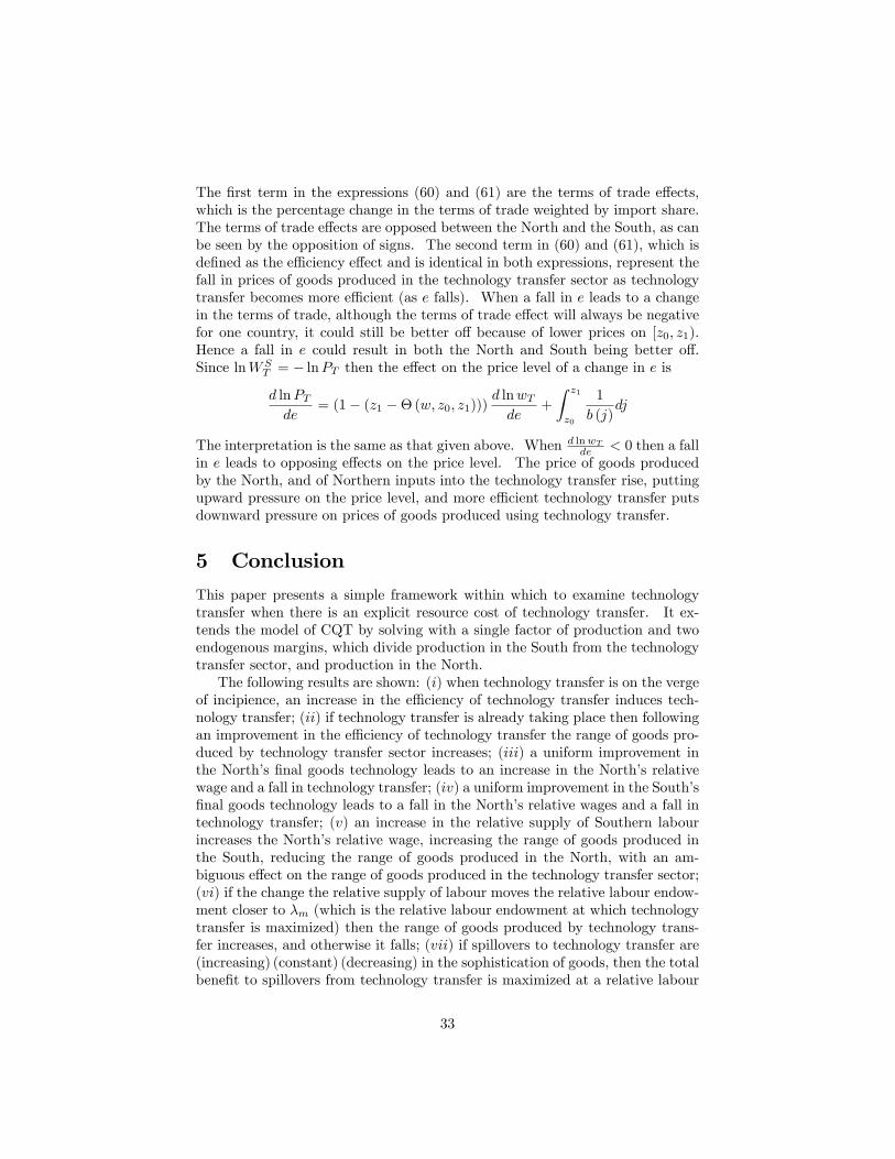
Production is allocated as demonstrated in Figure 1 with � indicating theboundary determined by (13) and � indicating the boundary determined by(14). Goods on the interval [0; z0) are produced in the South; goods on theinterval [z1; 1] are produced in the North; and goods on [z0; z1) are produced inthe South using Northern technology and both Northern and Southern labour.
3.5 DFS Benchmark
The comparative advantage locus is
w = a(z) (15)
7This ensures that production in each country, and production using transferred technology,occurs over contiguous regions of the goods continuum.
8This assumption requires that 2L0T (z0)�a0(z0)� wL0T (z0)
��
LT (z0)�a00(z0)� wL00T (z0)
�> 0 which is satis�ed when a00(z0) 6 wL00T (z0): When
a(z) and LT (z) are linear in z, the inequality holds as a00(z) and L00T (z) are both zero.
9

jz1
α
w, a(j)
1z00
a(j) b(j)
wT
1
β
e
Figure 1: Equilibrium with technology transfer
Labour market equilibrium in the South is determined by
LS = (1� z)wLN + (1� z)LS
which when rearranged gives an equation for the balance of trade
w =
�1� zz
�� (16)
where � = LS
LN. The balance of trade equation may be interpreted as the wage
which ensures balance of trade when the cut-o¤ good is z. Equilibrium in theDFS benchmark occurs at the intersection of the comparative advantage locusand the balance of trade locus (point in Figure 2). At this point trade isbalanced and the location of production is e¢ cient.An alternative way of examining the equilibrium involves inverting (15) so
that z = a�1(w) = z(w) where z0(w) > 0. Substituting this into (16) gives
w =
�1� z(w)z(w)
�� (17)
which is one equation in one unknown, w. This leads us to our �rst proposition.
Proposition 1 For each value of � 2 (0;1) there is a unique solution to theDFS-benchmark model denoted by (zD(�); wD(�)). As � increases, wD and zDincrease.
10

γ
w, a(j)
1zD0
a(j)
wD
1
BOTDFS
j
Figure 2: DFS benchmark model
hDFS(w)λ
w
hDFS(w)λ
hDFS(wD)λ
wD
Figure 3: Equilibrium in the DFS benchmark model
11

Proof. Since z0(w) > 0, and de�ning the RHS of (17) as hDFS (w)�, then
@hDFS(w)�@w < 0. The RHS of (17) is decreasing in w, while the LHS is increas-
ing in w. Also since as w approaches one then z approaches zero and thereforehDFS (w)� approaches in�nity, then hDFS (w)� > w for small w. This ensuresa unique equilibrium, denoted by the pair (zD(�), wD(�)). Since an increase in� will shift the hDFS (w)� locus outward, then w0D(�) > 0, and it follows thatz0D(�) > 0. See Figure 3.
Corollary 2 For any given pair (z (w) ; w) there exists a unique � which ensuresan equilibrium in the DFS-benchmark model.
Proof. This follows directly from equation (17).
3.6 Balance of Trade with Technology Transfer
We solve for the balance of trade by examining labour market equilibrium inthe South. The South engages in two types of productive activity. It pro-duces �nal goods on [0; z0) using Southern technology, and it provides labourwhich is combined with Northern labour and technology to produce goods on[z0; z1). We separate the total demand for Southern labour into LSD1 and L
SD2,
corresponding to the sub-intervals [0; z0) and [z0; z1). The demand for Southernlabour to produce a good j on [0; z0) is
LSD1(j) = a (j) :y(j) = a (j) :Y
p(j)= Y
since p(j) = a (j). The total demand for Southern labour to produce goodsj 2 [0; z0) is thus
LSD1 =
Z z0
0
Y = z0Y (18)
On the interval [z0; z1) each unit of good j requires the input of e units ofSouthern labour and LT (j) units of Northern labour according to (4). Giventhat the output of good j is Y
p(j) then
y(j) =Y
e+ wLT (j)(19)
and the derived demand for labour for good j is
LSD2(j) = ey(j) =eY
e+ wLT (j)(20)
Integrating over [z0; z1) yields
LSD2 =
Z z1
z0
eY
e+ wLT (j)(21)
= z1Y � z0Y � YZ z1
z0
wLT (j)
e+ wLT (j)dj
12

which gives the demand for Southern labour in the technology transfer sector.Equating the total demand for Southern labour (LSD1 + L
SD2) with the supply
of Southern labour�LS�gives the South�s labour market equilibrium
LS = z1Y � YZ z1
z0
wLT (j)
e+ wLT (j)dj (22)
We de�ne for convenience the following
�(j) =wLT (j)
e+ wLT (j)and (23)
�(w; z0; z1) =
Z z1
z0
�(j)dj (24)
where �(j) is the North�s factor share in good j, and �(w; z1; z0) is an expendi-ture share weighted sum of the North�s factor shares over [z0; z1).9 Hence �Yis the share of world expenditure spent on Northern resources for the purposesof technology transfer. Given that world income Y = LS + wLN , then (22)may be written
w =
�1� (z1 ��(w; z0; z1))z1 ��(w; z0; z1)
�:� (25)
which for given z0 and z1 determines the relative wage, w, which ensures bal-ance of trade. When there is no technology transfer, so that z1 = z0, then
�(w; z0; z1) = 0 and the balance of trade reduces to the DFS balance of tradeexpression (16).
3.7 Speci�cation of Model with Technology Transfer
The model may be expressed as three equations, (26), (27) and (28), in 3 un-knowns, w; z0; and z1.
a(z0) = wLT (z0) + e (26)
w = e+ wLT (z1) (27)
w =
�1� (z1 ��(w; z0; z1))z1 ��(w; z0; z1)
�:� (28)
9�(w; z1; z0) can also be thought of as the North�s average factor share for goods producedusing technology transfer on [z0; z1).
13

3.7.1 Properties of z0(w; e) and z1(w; e)
Equations (26) and (27) may be used to determine the responses of z0 and z1to changes in w and e. From (26), then10
z0w =dz0dwjdw=0 =
LT (z0)
a0(z0)� wL0T (z0)> 0 by A1 (29)
z0e =dz0dwjde=0 =
1
a0(z0)� wL0T (z0)> 0 by A1 (30)
and it follows that
z0 = z0(w+; e+) (31)
Di¤erentiating z0w with respect to w gives11
@z0w@w
= z0ww = LT (z0) (2L0T (z0)� z0w (a00(z0)� wL00T (z0))) > 0 by A2
Using (27) allows calculation of
z1w =dz1dwjde=0 =
(1� LT (z1))2eL0T (z1)
> 0 (32)
z1e =dz1dejdw=0 = �
(1� LT (z1))eL0T (z1)
< 0 (33)
and it follows that
z1 = z1(w+; e�) (34)
Di¤erentiating z1w with respect to w gives
@z1w@w
= z1ww =z1ww
�ez1e
L00T (z1)
L0T (z1)� 2�< 0 (35)
The functions z0(w; e) and z1(w; e) are drawn in Figure 4. For the z0 (w; e)locus, from (26), since wLT (z0) = a(z0) � e, then when w = 0 it followsthat aS(z0) = e, and the z�intercept is z0 = a�1(e):12 Further, by (A2),ddw
�dz0dw jde=0
�> 0, then z0(w; e) is increasing at a non-decreasing rate from the
intercept a�1(e). For the z1 (w; e) locus from (27), at w = e then LT (z1) = 0and z1 = 0. Since L0T (j) > 0 and L00T (j) > 0 then @z1w
@w < 0, and as w in-creases z1 is increasing at a decreasing rate. Since (27) may be rewrittenLT (z1) = 1� e
w then as w rises LT (z1) �! 1 and z1 asymptotes at L�1T (1) 6 1
since LT (1) 6 1. In Figure 4 both z0(w; e) and z1 (w; e) are drawn for a given
level of e. Since z1e < 0; as e falls the z1(w; e) locus shifts to the left. Similarly,because z0e > 0 then as e falls the z0(w; e) locus shifts to the right.13
10Note that by the Implicit Function Theorem dzidwjde=0 = @zi
@wand dzi
dejdw=0 = @zi
@e8i = 0; 1
11A2 may be assured by assuming that a00(z0) 6 wL00T (z0)12where a�1(:) is de�ned as the inverse function of a(:).13When e = 1 then the z � intercept for z0(w; e) is a�1(1) = 0, and the w � intercept for
z1(w; e) is 1.
14

z
we
LT1(1)
wH
zL
z0(w,e)
z1(w,e)
wL
zH
a1(e)
a1(w)
Figure 4: Representation of z1 (e; w) and z0 (e; w)
15

z
we*
LT1(1)
z*
z0(w, e*)
z1(w, e*)
a1(e*)
w*
a1(w)
BOTDFS(λ* )
Figure 5: z0 (w; e) and z1 (w; e) at e = e�
Proposition 3 There exists a value of e; de�ned as e�, such that for all valuesof e > e� there is no technology transfer, and the model reduces to the DFSbenchmark with solution (zD; wD).
Proof. e� is de�ned as level of e at which z0(w; e�) and z1(w; e�) are tan-gent, such that z1w (w�; e�) = z0w (w�; e�)14 and z0 (w�; e�) = z1 (w�; e�) = z�.Equations (26) and (27) reduce to w = a(z) and equation (28) becomes w =�1�zz
�LS
LN. The model reduces to the DFS benchmark, with equations (15) and
(16) ; and solutions (zD (�) ; wD (�)). This is drawn in Figure 5. For e > e� thecurves do not touch. Similarly, the solution is given by the DFS benchmark.
De�nition 4 The relative labour supply, ��, solves the DFS benchmark at(z� (w�) ; w�).
Appealing to Corollary 2, then �� solves (17) at (z� (w�) ; w�). TheBOTDFS (��)
locus is drawn in Figure 5.
Proposition 5 When e 2 [1; e�) there are two points of intersection betweenz0(w; e) and z1 (w; e) on [0; 1], which are de�ned (zL (wL) ; wL)and (zH (wH) ; wH) :Associated with each point of intersection is a relative labour endowment, �L (e)and �H (e) respectively. When � =2 (�L(e); �H(e)) then technology transfer doesnot occur, and the solution is given by the DFS benchmark.
14Note that a�1 (w) is also tangent to z0 (w; e�) and z1 (w; e�) at this point.
16

Proof. Given the properties of z0(w; e) and z1(w; e) there are two points ofintersection between the respective loci when e 2 [1; e�). At points of intersec-tion, z0(w; e) = z1(w; e), equations (26) and (27) reduce to w = a(z). Thatis,
z0 = z1 =) w = a (z) (36)
where z = z0 = z1. Where z0(w; e) and z1(w; e) intersect, it follows from (36)that z = z(w),15 and z(w) must also pass through the points of intersection.Further, it is the case that z0w (wL) < z0 (wL) < z1w (wL) and z0w (wH) >z0 (wH) > z1w (wH) :
16 The points of intersection are denoted (zL (wL) ; wL)and(zH (wH) ; wH).From Corollary 2, corresponding to (zL (wL) ; wL)and (zH (wH) ; wH) are
�L (e) and �H (e) respectively, which solve (17) for each case. Since zL (wL) <zH (wH) it follows that �L (e) < �H (e). If � 6 �L (e) or � > �H (e) thentechnology transfer will not occur as z1 6 z0; and the model reduces to the DFSbenchmark described by (15) and (16).
3.8 Solving the Model with Technology Transfer
Substituting (31) and (34) into (28) gives
w =
�1� z1(w; e) + �(w; z0(w; e); z1(w; e))z1(w; e)��(w; z0(w; e); z1(w; e))
�� (37)
which is one equation in one unknown, w, and determines the equilibrium tothe model when there is technology transfer. De�ning the RHS of (37) ash(w; e):�, the equilibrium of the model is determined by
w = h(w; e)� for all w 2 (wL (e) ; wH (e)) (38)
w = hDFS (w)� for all w 6 wL (e) ; w > wH (e) (39)
since from Proposition 3, the solution to the model is given by the DFS bench-mark for w 6 wL (e) ; w > wH (e). From Proposition 1, a unique equilibriumis ensured for w 6 wL (e) ; w > wH (e). To ensure the existence of a uniqueequilibrium for w 2 (wL (e) ; wH (e)) it is necessary to show that hw(w; e) < 0.
Unique Equilibrium: We di¤erentiate h(w; e) with respect to w: Let h(w; e) =1�vv where v = z1(w) � �(w; z0; z1). Then hw(w) = �vw
v2 , and it follows thatsign jhw(w)j = �sign jvwj. Thus, there is a unique equilibrium if hw(w) < 0=) vw > 0. To calculate vw = z1w(w)��w(w; z0; z1) requires �rst the appli-cation of Leibniz rule to determine �w.
�w =d�
dw=
d
dw
Z z1(w)
z0(w)
wLT (j)
e+ wLT (j)dj)
!
=e
w
Z z1
z0
� (j)
e+ wLT (j)dj + � (z1) :z1w � � (z0) :z0w (40)
15where z (w) = a�1 (w) :16 This is drawn in Figure 4.
17

jz1
1
1z00
θ(j,w1 )
θ(j )
θ(j,w2)
dz1dz0
w2 > w1
a
b c
d
Figure 6: Representation of hw
Intuitively, �(w; z0; z1) is an expenditure weighted sum of the factor sharesof Northern inputs in the technology transfer sector. As w increases there isadjustment to �(w; z0; z1) on three margins. Firstly, as w rises the North�sfactor share of any good j produced using technology transfer, � (j) ; rises. Thisis represented by the area a in Figure 6, and the �rst term in (40). Secondly,z1 will rise as the increase in w drives goods initially produced only in theNorth into the technology transfer sector, were they are produced with bothNorthern and Southern labour inputs (area c ; second term). Thirdly, z0 willrise as the fall in the relative price of Southern labour makes it economic toproduce goods on the z0 boundary using Southern labour only, as opposedto a combination of Southern and Northern labour in the technology transfersector (area b; third term). The �rst and second terms lead to an increase in�(w; z0; z1) while the third leads to a decrease, and in terms of the areas inFigure 6, �w = a+ c� b. Overall it is likely that an increase in w will lead toan increase in �(w; z0; z1),Since v = z1 ��(w; z0; z1) then vw is
vw = z1w (1� � (z1)) + � (z0) z0w �e
w
Z z1
z0
� (j)
e+ wLT (j)dj (41)
In terms of Figure 6, vw = d+ b� a. At both wL and wH , since z0 = z1(= z)then vw = (1� �(z)) z1w+�(z)z0w > 0. Since vw > 0 then h(w; e)� is negativelysloped at both wL and wH , although is not possible to establish whether theslope of h(w; e)� is greater or less than the slope of hDFS (w)� i.e. hw(w; e) ?
18

hDFSw(w).17
The term (z1 � �) is the South�s share of world income. As the wagerises, z1 increases shifting goods initially produced entirely in the North intothe technology transfer sector, where the factor share of Southern labour is1 � � (z1) : This increases the demand for Southern labour by (1 � �(z1))z1w:An increase in the wage also increases z0; which moves goods at that margin fromthe technology transfer sector to the South which also increases the demand forSouthern labour by �(z0))z0w. Finally the rise in w increases � (j) on [z0; z1);which is the North�s factor share of the inframarginal goods, which reduces thedemand for Southern labour, and is given by the term �
R z1z0
�(j)e+wLT (j)
dj. Theoverall e¤ect on South�s share of world income depends on the sum of theseterms as given in (41) :For w 2 (wL; wH) the third term in (41) is positive as z1 > z0, which leads
to the possibility that vw may become negative, and hw positive for some w 2(wL; wH). Although this is possible it is unlikely, and we henceforth make theassumption that vw > 0 for all w 2 (wL; wH) which ensures that hw(w; e) < 0.Since h (w; e)� is anchored at (wL; hDFS (wL)�)and (wH ; hDFS (wH)�) ; as inFigures 7 and 8, then given that hw (w; e) < 0 a unique equilibrium is assured.In addition it is likely that vww(wL) < 0 and so at wL the h(w) locus is
decreasing at a decreasing rate, and it is also possible that vww becomes positiveas w increases from wL leading to the possibility of an in�exion point on theinterval (wL; wH).18 Four possible shapes for the h(w; e) schedule, consistentwith the conditions above, are given in Figures 7 and 8.The points (zL (wL) ; wL) and (zH (wL) ; wH) are determined purely by tech-
nology and are not in�uenced by the relative labour endowment or tastes.Hence, an increase in � has the e¤ect of shifting h(w; e)� upward, withoutaltering wL or wH , as drawn in Figure 9.
3.9 E¤ect of a fall in e on the relative wage
Given (38) the e¤ect of a change in absorption on the relative wage is determinedby
dw
de=
he (w; e)
1� hw (w; e)(42)
It is thus necessary to calculate he (w; e) : Di¤erentiating h(w; e) with respectto e; where h(w; e) = 1�v
v and v = z1(w; e) � �(w; z0; z1) then he = � vev2 .
17At wi (i = L;H) it is the case that hDFSw (wi) = � z0(wi)z(wi)
2 and hw(wi; e) =
� (1��(z))z1w+�(z)z0wz(wi)
2 . At wL, z1w (wL) > z0 (wL) > z0w (wL) and at wH , z1w (wL) <
z0 (wL) < z0w (wL). Since ve is a weighted average of z1w (w) and z0w (w) ; it is not possibleto determine at either of these points whether (1� �(z)) z1w + �(z)z0w T z0 (wi).18See the Appendix for a further discussion.
19

w
hDFS (w)λ
wL wH wL wHwI
h(w,e)λ
h(w,e) λ
h(w,e)λ,hDFS(w)λ
hDFS (w)λ
h(w,e)λ,hDFS(w)λ
Figure 7: Possible shapes for h (w; e)
wHwL
h(w,e)λ
wH wwLw wI
h(w,e)λ
h(w,e)λ,hDFS(w)λ
h(w,e)λ,hDFS(w)λ
hDFS(w)λ hDFS(w)λ
Figure 8: Possible shapes for h (w; e)
20

h(w,e)λ
wwL
h(w,e)λ1
wH
h(w,e)λ0
λ0 < λ1
Figure 9: E¤ect of increase in � on h (w; e)�
Applying Leibniz Rule then
�e (w; z0; z1) =d�
de=d
de
Z z1(e)
z0(e)
wLT (j)
e+ wLT (j)dj
!
= �(z1)z1e � �(z0)z0e �Z z1
z0
� (j)
e+ wLT (j)dj < 0 (43)
Since � (j) falls as e increases then the change in integral of � (j) between z1and z0 as e increase is negative, and is represented by the third term in (43),and also by the area r in Figure 10. This represents an increase in the South�sfactor share of goods produced using technology transfer, as the South�s unitlabour requirement in the technology transfer sector increases. The �rst termin (43), �(z1)z1e(e); which is the area s; represents the fall in � as z1 falls inresponse to an increase in e; as the higher cost of production in the technologytransfer sector leads production to move from the technology transfer sectorto be produced by Northern labour only. The second term, �(z0)z0e; (area t)represents the decrease in � as z0 increases as higher costs of production usingtechnology transfer drive production to the South. In terms of the areas inFigure 10, �e = �r � s� t; and �e < 0. It follows that ve = z1e ��e is
ve = z1wdw
de+ (1� �(z1)) z1e + �(z0)z0e +
Z z1
z0
� (j)
e+ wLT (j)dj (44)
which is ambiguous in sign. It follows from (41) ; (42) and (44) that dwde =
21

j
1
1z00
θ(j,e1)
dz0 dz1
θ(j )
θ(j,e2)e2 > e1
z1
rs
t
q
Figure 10: Representation of he
� vev2+vw
and
dw
de= �
(1� �(z1)) z1e + �(z0)z0e +R z1z0
�(j)e+wLT (j)
dj
(z1 ��)2 + z1w (2� � (z1)) + � (z0) z0w � ew
R z1z0
�(j)e+wLT (j)
dj(45)
Since the denominator is positive,19 the sign of dwde is determined by the numer-ator. For a fall in e then z0 falls and goods on that margin that were initiallybeing produced entirely by the South are shifted to the technology transfer sec-tor and are produced with factor shares � (z) to (1� � (z)) by North and Southrespectively. Hence the demand for Southern labour falls by � (z0) z0e. On thez1 margin, goods that were initially produced entirely in the North shift into thetechnology transfer sector, to be produced by both the North and the South.This increases the demand for Southern labour by � (1� � (z1)) z1e: The fall ine reduces the South�s factor share of the inframarginal goods on [z0; z1) whichreduces the demand for Southern labour. This is the term �
R z1z0
�(j)e+wLT (j)
dj.Thus, whether the demand for Southern labour rises or falls depends on thesum of the terms in the numerator of (45). Figure 11 demonstrates the case ofdwde > 0: Using (45) it is now possible derive a number of additional propositions.
Proposition 6 From �L(e), �H (e) ;where e < e�; or from �� (e�), an im-provement in absorption (a fall in e) will lead to an increase (decrease) in w ifz1ez0e
< (>)� �(z)1��(z)
19Since hw (w; e) < 0 for w 2 (wL; wH) :
22

h(w,e)
ww1
h(w1,e1 )h(w,e1)
h(w,e2)
h(w2,e2 )
w2
e1 > e2
Figure 11: E¤ect of a fall in e on w
Proof. Initially the economy is at (zL; wL) ; (zH ; wH) ; or (z�; w�) and there isno technology transfer. Since z0 = z1 = z then (45) simpli�es to
dw
de= � (1� �(z)) z1e + �(z)z0e
z2 + z1w (2� � (z)) + � (z) z0w
and the sign��dwdw
�� = �sign j(1� �(z)) z1e + �(z)z0ej.For a fall in e then z0 falls, and goods on that margin that were initially
being produced entirely by the South shift into the technology transfer sector,which reduces the demand for Southern labour by �(z)z0e. On the z1 margin,goods that were initially produced entirely in the North shift into the technologytransfer sector, to be produced by both the North and the South. Hencethe demand for Southern labour rises by � (1� � (z)) z1e: Thus, whether thedemand for Southern labour rises or falls depends on � (1� �(z)) z1e��(z)z0e ?0. Figure 11 demonstrates the case of dwde > 0:The linear case (a (j) = 1 + j; LT (j) =
j2 ), which is solved in the Ap-
pendix, demonstrates an interesting case. At wL, it is the case that ve =(1� �(zL)) z1e (wL; e)+ �(zL)z0e (wL; e) < 0 and dw
de > 0: This is drawn in Fig-ure 12 (a). At wH it is the case that (1� �(zH)) z1e (wH ; e)+�(zH)z0e (wH ; e) >0 and dw
de < 0 (Figure 12 (b)). Hence a decrease in e from �L (e) leads to afall in the relative wage, while a decrease in e from �H (e) leads to a rise in therelative wage. Given that ve (wL) < 0 and ve (wL) > 0 it follows that there isa �w 2 (wL; wH) at which ve ( �w) = 0 and thusdwde = 0:
23

h(w)
wwL0
hDFS(w)λL
wH0wL
1 wH1
h(w)
wL0
hDFS(w)λH
wH0wL
1 wH1
(b)w
(a)
h(w,e1)λL
h(w,e1)λL
h(w,e0)λL
h(w,e0)λL
Figure 12: E¤ect of a fall in e in the linear case
It is now possible to show that technology transfer will occur when � 2(�L(e); �H (e)).
Proposition 7 From �L(e), �H (e) ;where e < e�; or from �� (e�), an improve-
ment in absorption (a fall in e) results in technology transfer (z1 � z0 > 0).
Proof. Initially there is no technology transfer and z0 = z1, and the economyis at (zL; wL) ; (zH ; wH) ; or (z�; w�). Suppose that there is a small fall in e.In response to this there may be a change in the relative wage and there arethree cases to consider:i. dwde > 0 : since z0 = z0(w; e), z0e > 0 and z0w > 0; then
dz0de
= z0wdw
de+ z0e > 0 (46)
This means that a fall in e leads to a fall in z0. The e¤ect on z1 = z1(w; e) isambiguous since z1w > 0, z1e < 0 and thus
dz1de
= z1wdw
de+ z1e ? 0 (47)
Setting dz1de = 0 de�nes a unique rate of change of the relative wage with respect
to e at which z1 is unchanged. From (47) this is
dw
dej�z1 = �
z1ez1w
> 0 (48)
24

The objective is to show that the equilibrium rise in the relative wage rises isless than dw
de j�z1 . Given the equilibrium condition, w = h(e; w), then since theeconomy is at �L(e), �H (e) ; or �
� (e�) then z0 = z1 = z and
dw
de=
he1� hw
= � (1� �(z)) z1e + �(z)z0ez2 + (2� �(z)) z1w + �(z)z0w
(49)
Taking the di¤erence dwde �
dwde j�z1 gives
dw
de� dwdej�z1 =
z1ez1w
� (1� �(z)) z1e + �(z)z0ez2 + (2� �(z)) z1w + �(z)z0w
(50)
=z2z1e + z1wz1e + � (z) z0wz1e � � (z) z0ez1w
z1w (z2 + (2� �(z)) z1w + �(z)z0w)< 0
Hence, dwde <dwde j�z1 it follows
dz1de < 0: A fall in e when dw
de > 0 leads to anincrease in z1 and a decrease in z0 and thus to technology transfer.ii. dwde < 0 : given that z1e < 0 and z1w > 0; then
dz1de
= z1wdw
de+ z1e < 0 (51)
a fall in e leads to a rise in z1. The e¤ect on z0 = z0(w; e) is ambiguous sincez0w > 0, z0e > 0 and thus
dz0de
= z0wdw
de+ z0e ? 0 (52)
Setting dz0de = 0 de�nes a unique rate of change of the relative wage with respect
to e at which z0 is unchanged. From (52) this is
dw
dej�z0 = �
z0ez0w
< 0
Taking the di¤erence dwde �
dwde j�z0 is
dw
de� dwdej�z0 =
z0ez0w
� (1� �(z)) z1e + �(z)z0ez2 + (2� �(z)) z1w + �(z0)z0w
=z2z0e + (2� � (z)) z1wz0e � (1� � (z)) z1ez0w
z0w (z2 + (2� �(z)) z1w + �(z)z0w)> 0
Since dwde >
dwde j�z0 it follows dz0
de > 0: A fall in e when dwde < 0 leads to an
increase in z1 and a decrease in z0 and thus to technology transfer.iii. dw
de = 0 : given that z1e < 0 and z0e > 0; then
dz1de
= z1e < 0
dz0de
= z0e > 0
25

A fall in e leads to a rise in z1 and a fall in z0 and thus to technology transfer.Hence, for all possible changes in the relative wage
�dwdw R 0
�; an improve-
ment in absorption from �L(e), �H (e) ;where e < e�; or �� (e�) leads to tech-nology transfer.
Proposition 8 From an initial equilibrium at which there is technology transfer(z1 � z0 > 0) then an improvement in absorption (a fall in e) results in anincrease in technology transfer.
Proof. From the appendix, given (72) and (73) then
dz0de
? 0 and dz1de
< 0
and from (74) thendz1de
� dz0de
< 0
and a fall in e leads to an increase in z1 � z0; and hence to an increase intechnology transfer.
Proposition 9 From an initial position at which there is technology transfer(z1 � z0 > 0) then a uniform improvement in the productivity of the Northern�nal goods sector leads to an increase in the relative wage and a contraction intechnology transfer
Proof. From the appendix, given (78) ; (79) ; (80) then
dw
d�N< 0;
dz0d�N
< 0 anddz1d�N
> 0
and hencedz1d�N
� dz0d�N
> 0
A uniform fall in aN (j) 8j from 1 ; which is a uniform improvement in Northern�nal goods technology, leads to an increase in the North�s relative wage, and adecrease in technology transfer.A uniform productivity improvement in Northern �nal goods sector shifts
the z1 margin to the left at the initial wage because production costs fall inthat sector. This increases the relative demand for Northern labour as goodsproduced originally on that margin using Northern and Southern labour in thetechnology transfer sector release Southern labour, and are now produced onlyin the North. This bids up the relative wage which increases z0 and decreases z1further. The movement between the initial and �nal equilibria are demonstratedin Figure 13 (with post-shock variables indicated by an *).
Proposition 10 From an initial position at which there is technology transfer(z1 � z0 > 0) then a uniform improvement in the productivity of the Southern�nal goods sector leads to a fall in the relative wage and a contraction in tech-nology transfer
26

jz1
w, a(j)
1z00
a(j)b(j,wT )ρN wT
1e
z1*
ρN* wT*
z0*
b(j,wT* )
ρN* < ρN=1
Figure 13: E¤ect of uniform productivity improvement in the North�s �nal goodssector
Proof. From the appendix, given (87) ; (88) ; (89) then
dw
d�S> 0;
dz0d�S
< 0; anddz1d�S
> 0
and hencedz1d�S
� dz0d�S
> 0
A uniform fall in a (j) 8j ; leads to a fall in the North�s relative wage, and adecrease in technology transfer.A uniform productivity improvement in the Southern �nal goods sector shifts
the z0 margin to the right at the initial wage because production costs fall inthat sector. This increases the relative demand for Southern labour as goodsproduced originally on that margin using Northern and Southern labour in thetechnology transfer sector release Northern labour as they move to be producedin the South. This pushes down the relative wage and decreases z1. Themovement between the initial and �nal equilibria are demonstrated in Figure14 (with post-shock variables indicated by an *).In DFS, a uniform proportional fall in the North�s unit labour requirements
has an equivalent impact to a proportional rise in the South�s unit labour re-quirements of the same size on the relative wage and cut-o¤ good.20 Whenthere is a technology transfer sector this equivalency fails. From Proposition 9,a uniform fall in the North�s unit labour requirements leads to an increase in w
20The e¤ect on absolute wages will di¤er.
27

jz1
w, a(j)
1z00
a(j)b(j,wT )
wT
1e
z1*
wT*
z0*
b(j,wT* )
a*(j) = ρSa(j)
a*(j)
Figure 14: E¤ect of uniform productivity improvement in the South�s �nal goodssector
and a fall in technology transfer, while from Proposition 10, a uniform rise inthe South�s unit labour requirements leads to an increase in w and an increasein technology transfer. Hence, the shocks have an asymmetric impact on thesize of the technology transfer sector.
Proposition 11 From an initial position at which there is technology transfer(z1 � z0 > 0) then a uniform improvement in all Northern productive technology,both in �nal goods and technology transfer, leads to an increase fall in both z0and z1:
Proof. From the Appendix, given (97) and (98) then
dz0d�N
> 0 anddz1d�N
> 0
however from (96) and (99)
dw
d�N? 0 and dz1
d�S� dz0d�S
? 0
A uniform fall in LT (j) and aN (j) 8j leads to a fall in z0 and z1; with anambiguous e¤ect on the relative wage and the size of the technology transfersector.
3.10 Increase in the relative supply of Southern labour, �
Since w = h(w; e):�, an increase in � shifts the h(w; e):� locus upward for anygiven w; as in Figure 9. This means that the equilibrium w increases, and it
28

follows from (29) and (32) that both z0 and z1 increase. The e¤ect on the rangeof goods in the technology transfer sector, z1 � z0; depends on z1w � z0w, andis examined in the next proposition.
Proposition 12 If e < e� there exists a relative labour endowment �m anda corresponding equilibrium (zm0 ; z
m1 ; wm) at which technology transfer is maxi-
mized. An increase or decrease in � from �m will reduce technology transfer.
Proof. Since expenditure shares are equal and constant for all goods, resourcesin technology transfer are maximized when z1�z0 is maximized. The functionsz1 (w; e) and z0 (w; e) are both twice continuously di¤erentiable, and intersectat wL and wH where wL < wH , with z0ww (w; e) > 0 8w and z1ww (w; e) < 08w: Since at wL it is the case that z0w (wL; e) < z1w (wL; e) and at wH it is thecase that z0w (wH ; e) > z1w (wH ; e) ; then there exists a wage wm on (wL; wH)de�ned by
d (z1 � z0)dw
= 0, z0w (wm; e) = z1w (wm; e)
at which z1 � z0 is maximized. Given (38) then �m is determined by
wm = h (wm; e)�m
An increase in � from �m leads to an increase in w and a fall in z1 � z0 asz0w (w; e) > z1w (w; e) for w > wm. A decrease in � from �m leads to a fall inw and a fall in z1 � z0 as z0w (w; e) < z1w (w; e) for w < wm.The intuition of this result is as follows. At one extreme, when the North�s
relative wage is very low, it is cheaper for the North to produce all goods abovez0 = z1 than to engage labour in technology transfer. At the other extreme,when Northern labour is very expensive it is cheaper for the South to produceall goods below z1 rather than to employ Northern labour in the technologytransfer sector.If population growth in the South is higher than in the North (� is increasing)
this drives up the price of Northern labour, pushing up z1 and z0. As wHis approached, z1w is falling and z0w is rising, and the range of goods overwhich technology transfer is taking place (z1 � z0) is falling. In the extreme,it is possible that the wage will rise enough to extinguish technology transferaltogether. This is counter to the result in CQT, which states as � increases therange of goods over which technology transfer occurs increases. This is a resultof the speci�cation of an external Northern factor that facilitates technologytransfer. This result is also counter to general mercantilist intuition, whichmight be stated as something like lower Southern wages increase the incentivefor the North to direct resources to technology transfer to the South to exploitthe opportunities created by cheaper Southern labour. However, as the Southernlabour forces expands, the opportunity cost of the resources used in technologytransfer (the Northern wage) rises, increasing the cost of producing goods usingtechnology transfer, encouraging production of �nal goods in the South usingonly Southern labour and technology.
29

3.10.1 Spillover Bene�ts to Technology Transfer
While the evidence on spillovers from FDI in developing countries is somewhatmixed, the possibility exists that technology transfer through FDI, or otherownership structure, may lead to spillovers bene�ts to other �rms in the sameindustry or in other industries.Spillover bene�ts could be increasing in j because spillovers increase with
technological sophistication. Alternatively spillovers may be decreasing in j be-cause �rms in high-tech sectors lack the absorptive capacity to assimilate ex-posure to new sophisticated technologies, while �rms in low-tech sectors, wherethe relative technological di¤erences are smaller, are more able to do so. Thefollowing proposition determines the location of the point of maximum spilloverbene�ts relative to �m depending on whether spillovers are increasing, constant,or decreasing in sophistication.
Proposition 13 Suppose that spillover bene�ts for good j 2 [z0; z1) are (increasing)(constant) (decreasing) in j; and are proportional to j�, � (>) (=) (<) 0: Thenthe total spillover bene�t to technology transfer is B =
R z1z0j�dj, which is maxi-
mized when �B (>) (=) (<)�m:
Proof. B is maximized at dBdw = 0 where B =
R z1z0j�dj =
z�+11 �z�+10
�+1 : Themaximum spillover bene�t occur at wB which is de�ned by
z1w (wB ; e)
z0w (wB ; e)=
�z0 (wB ; e)
z1 (wB ; e)
��From the properties of z0 (w; e) and z1 (w; e) and from Proposition 9 whichde�nes wm; then
z0w (w; e) > z1w (w; e) for w > wmz0w (w; e) = z1w (w; e) for w = wmz0w (w; e) < z1w (w; e) for w < wm:
If � > 0 then z1w(wB ;e)z0w(wB ;e)
< 1 and wB > wm: If � = 0 thenz1w(wB ;e)z0w(wB ;e)
= 1 and
wB = wm: If � < 0 then z1w(wB ;e)z0w(wB ;e)
> 1 and wB < wm: Since from (38) thereis a unique mapping between � and w; which is increasing, then it follows thatwhen � (>) (=) (<) 0 then �B (>) (=) (<)�m.Depending on whether spillover bene�ts are increasing, constant, or decreas-
ing in j determines whether the maximum spillover bene�t occurs above, at, orbelow the point of maximum technology transfer, de�ned by (wm; �m) :
30

4 Prices and Welfare
4.1 Prices
The price level in the pre-technology transfer situation is21
lnPD =
Z 1
0
ln pD(j) =
Z zD
0
ln a (j) dj + (1� zD) lnwD (53)
When there is technology transfer, the price level is
lnPT =
Z z0
0
ln a (j) dj +
Z z1
z0
ln b(j)dj + (1� z1) lnwT (54)
The di¤erence in the price level is
lnPT�lnPD = (1�zD) lnwTwD
+
Z zD
z0
(ln b (j)� ln a(j)) dj+Z z1
zD
(ln b(j)� lnwT ) dj
(55)Since b (j) < a(j) on [z0; zD) and b(j) < wT on [zD; z1) then the second andthird terms are negative. The �rst term represents the change in the prices ofgoods on [z1; 1] which depends on wT
wDand may be positive or negative. Hence
the change in the price level between the pre-technology transfer and technologytransfer equilibria is ambiguous.
4.2 Global Welfare
Totally di¤erentiating the expression for world income Y = wLN + LS gives
(1� zD)dw
w=dY
Y
and hence
(1� zD) ln�wTwD
�= ln
�YTYD
�Substituting this into (55) then
ln
�YTPT
�� ln
�YDPD
�=
Z zD
z0
(ln a (j)� ln b(j)) dj +Z z1
zD
(lnwT � ln b(j)) dj > 0
and world income Yi de�ated by the price index Pi (for i = T;D) increasesbetween the pre- and post-technology transfer situations.
21The subscript D denotes the DFS benchmark (pre-technology transfer situation), and thesubscript T denotes the technology transfer situation.
31

4.3 Welfare in the North and South
Without technology transfer, from (11) welfare per capita in the North is22
WND = lnwD �
Z 1
0
ln pD(j) = zD lnwD �Z zD
0
ln a(j)dj
Once technology transfer has occurred, Northern welfare per capita is
WNT = z1 lnwT �
Z z0
0
ln a (j) dj �Z z1
z0
ln b(j)dj (56)
The change in welfare per capita in the North is
�WN =WNT �WN
D = zD lnwTwD
+
Z zD
z0
(ln a (j)� ln b (j)) dj+Z z1
zD
(lnwT � ln b (j)) dj
(57)Since a (j) > b(j) on [z0; zD) and wT > b(j) on [zD; z1) then the second and thirdterms, which are the e¢ ciency gains due to technology transfer, are positive.The term zD ln
wTwD
is the terms of trade e¤ect, where zD is the North�s importshare in the pre-technology transfer equilibrium. If the Northern terms of trade
does not fall�wTwD
> 1�then the North is unambiguously better o¤ as a result
of technology transfer. From (12) ; welfare per capita in the South is initially
WSD = �
Z 1
0
pD(j) = �(1� zD) lnwD �Z zD
0
ln a (j) dj
and once technology transfer has occurred it is
WST = �(1� z1) lnwD �
Z z0
0
ln a (j) dj �Z z1
z0
ln b(j)dj (58)
The change in welfare per capita in the South is
�WS =WST �WS
D = �(1�zD) lnwTwD
+
Z zD
z0
(ln a (j)� ln b (j)) dj+Z z1
zD
(lnwT � ln b(j)) dj
(59)The interpretation of terms in (59) is the same as that for (57).
4.4 E¤ect of a Change in e on Welfare and Prices
In this section we examine the e¤ect of a fall in e on welfare and prices intechnology transfer equilibrium. Di¤erentiating (56) and (58) with respect toe gives
dWN
de= (z1 ��(w; z0; z1))
d lnwTde
�Z z1
z0
1
b (j)dj (60)
anddWS
de= � (1� (z1 ��(w; z0; z1)))
d lnwTde
�Z z1
z0
1
b (j)dj (61)
22W ij (i = N;S) is de�ned as ln
�UijPj
�from (11) and (12) ; for j = D;T .
32
The �rst term in the expressions (60) and (61) are the terms of trade e¤ects,which is the percentage change in the terms of trade weighted by import share.The terms of trade e¤ects are opposed between the North and the South, as canbe seen by the opposition of signs. The second term in (60) and (61), which isde�ned as the e¢ ciency e¤ect and is identical in both expressions, represent thefall in prices of goods produced in the technology transfer sector as technologytransfer becomes more e¢ cient (as e falls). When a fall in e leads to a changein the terms of trade, although the terms of trade e¤ect will always be negativefor one country, it could still be better o¤ because of lower prices on [z0; z1).Hence a fall in e could result in both the North and South being better o¤.Since lnWS
T = � lnPT then the e¤ect on the price level of a change in e is
d lnPTde
= (1� (z1 ��(w; z0; z1)))d lnwTde
+
Z z1
z0
1
b (j)dj
The interpretation is the same as that given above. When d lnwTde < 0 then a fall
in e leads to opposing e¤ects on the price level. The price of goods producedby the North, and of Northern inputs into the technology transfer rise, puttingupward pressure on the price level, and more e¢ cient technology transfer putsdownward pressure on prices of goods produced using technology transfer.
5 Conclusion
This paper presents a simple framework within which to examine technologytransfer when there is an explicit resource cost of technology transfer. It ex-tends the model of CQT by solving with a single factor of production and twoendogenous margins, which divide production in the South from the technologytransfer sector, and production in the North.The following results are shown: (i) when technology transfer is on the verge
of incipience, an increase in the e¢ ciency of technology transfer induces tech-nology transfer; (ii) if technology transfer is already taking place then followingan improvement in the e¢ ciency of technology transfer the range of goods pro-duced by technology transfer sector increases; (iii) a uniform improvement inthe North�s �nal goods technology leads to an increase in the North�s relativewage and a fall in technology transfer; (iv) a uniform improvement in the South�s�nal goods technology leads to a fall in the North�s relative wages and a fall intechnology transfer; (v) an increase in the relative supply of Southern labourincreases the North�s relative wage, increasing the range of goods produced inthe South, reducing the range of goods produced in the North, with an am-biguous e¤ect on the range of goods produced in the technology transfer sector;(vi) if the change the relative supply of labour moves the relative labour endow-ment closer to �m (which is the relative labour endowment at which technologytransfer is maximized) then the range of goods produced by technology trans-fer increases, and otherwise it falls; (vii) if spillovers to technology transfer are(increasing) (constant) (decreasing) in the sophistication of goods, then the totalbene�t to spillovers from technology transfer is maximized at a relative labour
33

supply which is (>) (=) (<)�m; (viii) the e¤ect of an increase in the e¢ ciencyof technology transfer on Northern and Southern workers�welfare depends ona terms of trade e¤ect, which is opposed between countries, and an e¢ ciencye¤ect which bene�ts both groups, and hence it is possible that both countriescould gain from an improvement in the e¢ ciency of technology transfer; (ix)comparing welfare between the pre-technology transfer and technology transferequilibria, the welfare consequences for the North and South are ambiguous,however world welfare increases.
Future Research: Future re�nements to this model include examiningpolicies that a¤ect technology transfer, for example subsidizing the resourcecost of technology transfer (LT ), or subsidizing the input of Southern labour.This presents an opportunity to examine the e¤ects of such policy in a generalequilibrium. The model also presents a framework for analyzing the interac-tion between FDI and immigration. If Southern labour is imperfectly mobilebetween the North and the South because of frictions such as immigration re-strictions, language and cultural di¤erences and the cost of relocation then thereis a wage, wim > 1; at which immigration �ows are zero. A fall in e leadingto an increase in technology transfer, and a rise or a fall in the relative wagewould then induce positive or negative immigration �ows. Other simple ex-tension include the case in which Northern and Southern workers have di¤erentpreferences and hence there is a demand side impact to shocks that alter theequilibrium, or requiring that Northern workers must attain some human capital(skills) in order to work in the technology transfer sector.
6 References
Aitken, Brian J. and Harrison, Ann E., 1999, �Do Domestic Firms Bene�t fromDirect ForeignInvestment? Evidence from Venezuela,�American Economic Re-view, 89(3), pp. 605-618.Baldwin, Richard and Frederic Robert-Nicoud, 2007, "O¤shoring: General
Equilibrium E¤ects on Wages, Production and Trade," NBER Working PaperNo. 12991.Cheng, Leonard K., Qui, Larry D., Tan, Guofu, 2005, "Foreign direct invest-
ment and international trade in a continuum Ricardian trade model," Journalof Development Economics, 77, pp. 477-501.Damijan, Joze P., Mark Knell, Boris Majcen and Matija Rojec, 2003, �The
role of FDI, R&D accumulation and trade in transferring technology to tran-sition countries: evidence from �rm panel data for eight transition countries,�Economic Systems, 27, pp. 189-204.Djankov, Simeon and Hoekman, Bernard, 2000, �Foreign Investment and
Productivity Growth in Czech Enterprises,� World Bank Economic Review,14(1), pp. 49-64.Dornbusch, Rudiger, Fischer, Stanley, and Samuelson, Paul, 1977, �Compar-
ative Advantage, Trade and Payments in a Ricardian Model with a Continuum
34

of Goods,�American Economic Review, 67, pp. 823-39.Flam, Harry, and Helpman, Elhanan, 1987, "Vertical Product Di¤erentiation
and North-South Trade." American Economic Review, pp 810-22.Glass, Amy Jocelyn, and Saggi, Kamal, 2008, "The Role of Foreign Direct
Investment in International Technology Transfer," International Handbook ofDevelopment Economics, Vol. II.Grossman, Gene and Esteban Rossi-Hansberg, 2008, "Trading Tasks: A
Simple Theory of O¤shoring," American Economic Review, 98, No. 5, pp.1978-1997.Haddad, Mona and Harrison, Ann E. , 1993, �Are There Positive Spillovers
from Direct Foreign Investment�Evidence from Panel Data for Morocco,�Jour-nal of Development Economics, 42(1), pp 51-74.16Haskel, Jonathan E., Pereira, Sonia, and Slaughter, Matthew J., 2002, "Does
Inward Foreign Direct Investment Boost the Productivity of Domestic Firms?,"NBER Working paper No. 8724.Javorcik, Beata Smarzynska, 2004, "Does Foreign Direct Investment Increase
the Productivity of Domestic Firms? In Search of Spillovers through Backwardlinkages," American Economic Review 94, pp 605-627.Jones, Ronald W., and Ru¢ n, Roy, 2007, �International Technology Trans-
fer: Who Gains and Who Loses?,�Review of International Economics, 75, No.2, pp 321-328.Jones, Ronald W., and Ru¢ n, Roy, 2008, �The Technology Transfer Para-
dox,�Journal of International Economics, 15, No. 2, pp 209-222.Kinoshita, Yuno., 2000, �R&D and Technology Spillovers via FDI: Innova-
tion and Absorptive Capacity,�CEPR Discussion Paper No. 2775.Konings, Jozef and Alan Murphy, 2001, �Do Multinational Enterprises Sub-
stitute Parent Jobs for Foreign Ones? Evidence from European Firm-LevelPanel Data,�CEPR Discussion Paper No. 2972.Krugman, Paul, 1979, "A Model of Innovation, Technology Transfer, and
the World Distribution of Income," Journal of Political Economy, 87, No. 2, pp.253-266.Mussa, Michael, 1978, "Dyanmic Adjustment in the Heckscher-Ohlin-Samuelson
Model," Journal of Political Economy, 86, No. 5, pp. 775-791.Rodriguez-Clare, 2010, "O¤shoring in a Ricardian World," American Eco-
nomic Journal: Macroeconomics, Vol. 2, No. 2.Samuelson, Paul A., 2004, �Where Ricardo and Mill Rebut and Con�rm
Arguments of Mainstream Economists Supporting Globalization,� Journal ofEconomic Perspectives, 18, No. 3, pp. 135-46.Stokey, Nancy L., 1991, "The Volume and Composition of Trade between
Rich and Poor Countries." Rev. Econ. Studies 58, pp. 63-80.Teece, D.J., 1977, "Technology Transfer by Multinational Firms: The Re-
source Cost of Transferring Technological Know-How," Economic Journal, 87,pp. 242-261.
35

7 Appendix
7.1 Solution to the Model in the Linear Case
We now solve the model for the simple linear case as a demonstration
a(j) = 1 + j
LT (j) =j
2
It follows that b(j) = e + w j2 : The boundaries of production, z0 and z1; are
de�ned a(z0) = b(z0) =, and w = b(z1) which give
z0(w; e) =2e� 22� w (62)
z1(w; e) =2(w � e)w
(63)
Since z0 2 [0; 1] then w < 2. Taking the �rst and second derivatives withrespect to w gives
z0w(w; e) =2(e� 1)(2� w)2
z0ww(w; e) =2(2e� 2)(2� w)3 > 0 for all w < 2
z1w(w; e) =2e
w2
z1ww(w; e) = � 4ew3
< 0
and �rst derivatives with respect to e gives
z0e(w; e) =2
2� w > 0
z1e(w; e) = � 2w< 0
The balance of trade is
w =
0@1� z0 � 2ew ln
�2e+wz12e+wz0
�z0 +
2ew ln
�2e+wz12e+wz0
�1A� (64)
The model may be described by three equations, (62) ; (63) and (64) in threeunknowns (w; z0; z1).Substituting for z0 and z1 using (62) and (63) into (64) ; and setting � = 1
for simplicity leads, gives
w = h(w; e)� =
0@1� 2e�22�w �
2ew ln
�2w�w22e�w
�2e�22�w +
2ew ln
�2w�w22e�w
�1A
36

which is one equation in one unknown, w. Solving wL and wH by settingz0 = z1 using (62) and (63) gives
2e� 22� w =
2w � 2ew
, w2 � 3w + 2e = 0
wL = 1:5� 12(9� 8e)
12 (65)
wH = 1:5 +1
2(9� 8e)
12 (66)
Solving for e�, which occurs when wL = wH , requires that 8e = 9 so that
e� = 1:125
w� = 1:5
z� = 0:5
Given that w� = 1:5 and z� = 0:5 then �� = 1:5: Solving the model for aparticular e < e�; we set e = 1:1. The solving for wL and wH gives
wL = 1:2764
wH = 1:7236
In addition, z1ww (wL) > 0 and z1ww (wH) < 0 with a point of in�exion(z1www = 0) at wI = 1:6238. Because of the point of in�exion, the h (w; e)�intersects the hDFS (w)� curve at 1:5092 ; and lies below it on the interval(1:2764; 1:5092) ; and above it over the interval (1:5092; 1:7236).The DFS benchmark model is
a(z) = 1 + z (67)
w =
�1� zz
�� (68)
Substituting (67) into (68), with � = 1; gives
w = hDFS(w) =2� ww � 1
The solution to the DFS benchmark is
w = (2)1=2 = 1:4142
z = (2)1=2 � 1 = 0:4142
7.2 Di¤erentiating h(w; e) with respect to w
Let h(w; e) = 1�vv where v = z1(w)��(w; z0; z1). Then
hw(w) =�vwv2
37

It follows thatsign jhw(w)j = �sign jvwj
To calculate vw = z1w(w) � �w(w; z0; z1) requires the application of Leibnizrule to determine �w.
�w =d�
dw=
d
dw
Z z1(w)
z0(w)
wLT (j)
e+ wLT (j)dj)
!
=
Z z1
z0
d
dw
�wLT (j)
e+ wLT (j)
�dj +
wLT (z1)
e+ wLT (z1):z1w �
wLT (z0)
e+ wLT ((z0):z0w
=
Z z1
z0
LT (j)
e+ wLT (j)dj �
Z z1
z0
wLT (j)2
(e+ wLT (j))2 dj + � (z1) :z1w � � (z0) :z0w
=1
w
Z z1
z0
�� (j)� � (j)2
�dj + � (z1) :z1w � � (z0) :z0w
=1
w�(w; z0; z1)�
1
w
Z z1
z0
� (j)2dj + � (z1) :z1w � � (z0) :z0w
=e
w
Z z1
z0
� (j)
e+ wLT (j)dj + � (z1) :z1w � � (z0) :z0w
7.2.1 Calculating vww at wL and wH
vww =ez1ww
e+ wLT (z)+wLT (z)z0wwe+ wLT (z)
+eLT (z)
(e+ wLT (z))2(z0w � z1w) +
ewL0T (z)
(e+ wLT (z)2�(z0w)
2 � (z1w)2�
= (1� �(z)) z1ww�
+ �(z)z0ww+
+eLT (z)
(e+ wLT (z))2(z0w � z1w) +
ewL0T (z)
(e+ wLT (z)2�(z0w)
2 � (z1w)2�
Substituting for z0ww and z1ww gives
vww = (1� �(z)) (1� LT (z1))e
@z1@w
�2� (1� LT (z1))
(L0T (z1))2 L00T (z1)
!
+�(z)LT (z0)
�2L0T (z0)� LT (z0)
�a00(z0)� wL00T (z0)a0(z0)� wL0T (z0)
��+
eLT (z)
(e+ wLT (z))2(z0w � z1w) +
ewL0T (z)
(e+ wLT (z)2�(z0w)
2 � (z1w)2�
At wL, z1w > z0w > 0 and so
vww = (1� �(z)) z1ww�+�(z)z0ww
++
eLT (z)
(e+ wLT (z))2
�z0w � z1w
�
�+
ewL0T (z)
(e+ wLT (z)2
�(z0w)
2 � (z1w)2�
�At wH , 0 < z1w < z0w and so
vww = (1� �(z)) z1ww�+�(z)z0ww
++
eLT (z)
(e+ wLT (z))2
�z0w � z1w
+
�+
ewL0T (z)
(e+ wLT (z)2
�(z0w)
2 � (z1w)2+
�
38

It is likely that vww(wL) < 0 and vww(wH) > 0, although this cannot be shownwith certainty without making further restrictions on the general functionalforms. What does that mean about h(w)?Since h(w) = 1�v
v , where v = z1(w)��(w; z1; z0) and hw(w) = �vwv2 then
hww =�v2:vww + 2v:(vw)2
v4=1
v2
�2(vw)
2
v� vww
�This means that if vww < 0 then hww > 0, and if vww > 0 then hww ? 0. Sinceit is likely that vww(wL) < 0 then hww(wL) > 0 and h(w) is decreasing at adecreasing rate at this point. If hww(w) falls below zero as w increases towardswH , then h(w) is decreasing at a decreasing rate near wL, and decreasing atan increasing rate for some w > wL. Thus, there would a point of in�exion,hww = 0, at wI where wL < wI < wH . This turns out to be the case for thesimple linear functional forms examined in the special case.
7.3 Di¤erentiating h (w; e) with respect to e
�e =d�
de=d
de
Z z1(e)
z0(e)
wLT (j)
e+ wLT (j)dj
!
=
Z z1
z0
d
de
�wLT (j)
e+ wLT (j)
�dj + �(z1):z
01(e)� �(z0):z00(e)
= �(z1):z1e(e)� �(z0):z0e(e)�Z z1
z0
� (j)
e+ wLT (j)dj
7.3.1 Di¤erentiating z0e and z1e with respect to w
From (30), di¤erentiating z0e with respect to w gives
z0ew = �a00(z0)� wL00T (z0)� L0T (z0)
(a0(z0)� wL0T (z0))2 > 0 by A2 (69)
From (33) ; di¤erentiating z1e with respect to w gives
z1ew =eL0T (z1)
2+ (1� LT (z1)) eL00T (z1)(eL0T (z1))
2 > 0 (70)
39

7.4 Proof of Proposition 8: Improvement in Absorptionwith z1 � z0 > 0
Totally di¤erentiating the system (26) ; (27), and (28) ; where v = z1��(w; z0; z1)then 264
�1� �
v2ew
R z1z0
�(j)b(j)dj
��v2 � (z0)
�v2 (1� � (z1))
Lv (z0) � (a0 (z0)� wL0T (z0)) 01� LT (z1) 0 �wL0T (z1)
37524 dwdz0dz1
35
=
24 � �v2
R z1z0
�(j)b(j)dj
�11
35 deThe determinant is
� =
1� �
v2e
w
Z z1
z0
� (j) dj
(e+ wLT (j))2 dj
!(a0 (z0)� wL0T (z0))wL0T (z1)
+�
v2� (z0)wLT (z0)L
0T (z1)
+�
v2(1� � (z1)) (1� LT (z1)) (a0 (z0)� wL0T (z0)) > 0
It follows that
dw
de=
1
�
� �v2
�R z1z0
�(j)b(j)dj
�(a0 (z0)� wL0T (z0))wL0T (z1)
� �v2 � (z0)wL
0T (z1) +
�v2 (1� � (z1)) (a
0 (z0)� wL0T (z0))
!? 0(71)
dz0de
=1
�
0BB@�1� �
v2ew
R z1z0
�(j)b(j)dj
�wL0T (z1)
� �v2
�R z1z0
�(j)b(j)dj
�LT (z0)wL
0T (z1)
�v2 (1� � (z1)) (1 + LT (z0)� LT (z1))
1CCA ? 0 (72)
dz1de
=1
�
0B@ ��1� �
v2ew
R z1z0
�(j)b(j)dj
�(a0 (z0)� wL0T (z0))
� �v2 � (z0) (1 + LT (z0)� LT (z1))
� �v2
R z1z0
�(j)b(j)dj (1� LT (z1)) (a
0 (z0)� wL0T (z0))
1CA < 0 (73)
dz1de
� dz0de
=1
�
0BBB@�1� �
v2ew
R z1z0
�(j)b(j)dj
�(� (a0 (z0)� wL0T (z0))� wL0T (z1))
�v2 (1 + LT (z0)� LT (z1)) (�1� � (z0) + � (z1))� �v2
R z1z0
�(j)b(j)dj (1� LT (z1)) (a
0 (z0)� wL0T (z0))� �v2 (1� � (z1)) (1 + LT (z0)� LT (z1))
1CCCA < 0(74)
40

7.5 Proof of Proposition 9: Productivity North�s �nalgoods sector
The system of equations becomes
a(z0) = e+ wLT (z0) (75)
�Nw = e+ wLT (z1) (76)
w =
�1� (z1 ��(w; z0; z1))z1 ��(w; z0; z1)
�:� (77)
where initially �N = 1 in the initial state to adhere to the assumption thataN (j) = 1 for all goods j. Totally di¤erentiating the system of equations(holding e �xed) gives264
�1� �
v2ew
R z1z0
�(j)b(j)dj
��v2 � (z0)
�v2 (1� � (z1))
LT (z0) � (a0 (z0)� wL0T (z0)) 0�N � LT (z1) 0 �wL0T (z1)
37524 dwdz0dz1
35=
24 00�w
35 d�NThe determinant is
� =
1� �
v2e
w
Z z1
z0
� (j) dj
(e+ wLT (j))2 dj
!(a0 (z0)� wL0T (z0))wL0T (z1)
+�
v2� (z0)wLT (z0)L
0T (z1)
+�
v2(1� � (z1))
��N � LT (z1)
�(a0 (z0)� wL0T (z0)) > 0
Applying Cramer�s Rule then
dw
d�N=
1
�
�� �v2(1� � (z1))w (a0 (z0)� wL0T (z0))
�< 0 (78)
dz0d�N
= � 1�
��
v2(1� � (z1))LT (z0)w
�< 0 (79)
dz1d�N
=1
�
�1� �
v2ew
R z1z0
�(j)b(j)dj
�(a0 (z0)� wL0T (z0))w
+ �v2 � (z0)wLT (z0)
!> 0(80)
dz1d�N
� dz0d�N
=1
�
�1� �
v2ew
R z1z0
�(j)b(j)dj
�(a0 (z0)� wL0T (z0))w
+ �v2wLT (z0) (1 + � (z0)� � (z1))
!> 0(81)
A uniform improvement in Northern �nal goods technology�a fall in �N
�leads
to an increase in the North�s relative wage and a fall in technology transfer.
41

7.6 Proof of Proposition 10: Productivity of the South�s�nal goods sector
The system of equations becomes
�Sa(z0) = e+ wLT (z0) (82)
w = e+ wLT (z1) (83)
w =
�1� (z1 ��(w; z0; z1))z1 ��(w; z0; z1)
�� (84)
where initially �S = 1. Totally di¤erentiating the system of equations, holdinge �xed, leads to264
�1� �
v2ew
R z1z0
�(j)b(j)dj
��v2 � (z0)
�v2 (1� � (z1))
LT (z0) ���Sa0 (z0)� wL0T (z0)
�0
1� LT (z1) 0 �wL0T (z1)
37524 dwdz0dz1
35=
24 0a (z0)0
35 d�S (85)
We maintain A1 and hence �Sa0 (z0)� wL0T (z0) > 0: The determinant is
� =
1� �
v2e
w
Z z1
z0
� (j) dj
(e+ wLT (j))2 dj
!��Sa0 (z0)� wL0T (z0)
�wL0T (z1)(86)
+�
v2� (z0)wLT (z0)L
0T (z1)
+�
v2(1� � (z1)) (1� LT (z1))
��Sa0 (z0)� wL0T (z0)
�> 0
Applying Cramer�s Rule then
dw
d�S=
1
�
��
v2� (z0) a (z0)wL
0T (z1)
�> 0 (87)
dz0d�S
= � 1�
��1� �
v2e
w
Z z1
z0
� (j)
b (j)dj
�a (z0)wL
0T (z1)
�< 0 (88)
dz1d�S
=1
�
��
v2� (z0) a (z0) (1� LT (z1))
�> 0 (89)
dz1d�S
� dz0d�S
=1
�
�v2 � (z0) a (z0) (1� LT (z1))
+�1� �
v2ew
R z1z0
�(j)b(j)dj
�a (z0)wL
0T (z1)
!> 0 (90)
A uniform improvement in Southern �nal goods technology�a fall in �S
�leads
to a fall in technology transfer.
42

7.7 Proof of Proposition 11: Productivity of all NorthernTechnology
The system of equations is
a(z0) = e+ �NwLT (z0) (91)
�Nw = e+ �NwLT (z1) (92)
w =
�1� (z1 ��(w; z0; z1))z1 ��(w; z0; z1)
�:� (93)
where �(w; z0; z1) =R z1z0
�NwLT (j)e+�NwLT (j)
dj. Totally di¤erentiating the system leadsto 264
�1� �
T 2e�N
w
R z1z0
�(j)b(j)dj
��T 2 � (z0)
�T 2 (1� � (z1))
�NLT (z0) ��a0 (z0)� w�NL0T (z0)
�0
�N (1� LT (z1)) 0 ��NwL0T (z1)
37524 dwdz0dz1
35
=
24 �T 2 e
R z1z0
�(j)b(j)dj
�wLT (z0)�w (1� LT (z1))
35 d�N (94)
The determinant is
� =
�1� �
T 2e�N
w
Z z1
z0
� (j)
b (j)dj
��a0 (z0)� w�NL0T (z0)
�w�NL0T (z1)(95)
+�
T 2� (z0) �
NLT (z0) �NwL0T (z1)
+�
T 2(1� � (z1)) �N (1� LT (z1))
�a0 (z0)� w�NL0T (z0)
�and using Cramer�s Rule then
dw
d�N=
1
�
0B@ �T 2 e
�R z1z0
�(j)b(j)dj
� �a0 (z0)� w�NL0T (z0)
�w�NL0T (z1)
� �T 2 � (z0)wLT (z0) �
NwL0T (z1)� �T 2 (1� � (z1))w (1� LT (z1))
�a0 (z0)� w�NL0T (z0)
�1CA ? 0(96)
= � w
�N+1
�
�a0 (z0)� w�NL0T (z0)
�w�NL0T (z1) ? 0
dz0d�N
=1
�
�w2�NLT (z0)L
0T (z1)
�(97)
dz1d�N
=1
�
�w�a0 (z0)� w�NL0T (z0)
�(1� LT (z1))
�> 0 (98)
dz1d�N
� dz0d�N
=w
�
� �a0 (z0)� w�NL0T (z0)
�(1� LT (z1))
�w�NLT (z0)L0T (z1)
�? 0 (99)
43

7.8 Prices and Welfare
The di¤erence between prices when there is technology transfer and prices inthe pre-technology transfer situation is
lnPT � lnPD =
Z z0
0
ln a (j) dj +
Z z1
zD
ln b(j)dj + (1� z1) lnwT �Z zD
0
ln a (j) dj � (1� zD) lnwD(100)
= (1� z1) lnwT � (1� zD) lnwD +Z zD
z0
(ln b (j)� ln a(j))dj +Z z1
zD
ln b(j)dj)
= (1� zD) lnwTwD
+
Z zD
z0
(ln b (j)� ln a(j)) dj +Z z1
zD
(ln b(j)� lnwT ) dj
Without technology transfer, welfare in the North
WND = lnwD�
Z 1
0
ln pD(j) = lnwD�Z zD
0
ln a(j)dj�Z 1
zD
lnwDdj = zD lnwD�Z zD
0
ln a(j)dj
Once technology transfer has occurred, Northern welfare is
WNT = lnwT �
Z 1
0
ln pT (j) = lnw �Z z0
0
ln a (j) dj �Z z1
z0
ln b(j)dj �Z 1
z1
lnwT dj
= z1 lnwT �Z z0
0
ln a (j) dj �Z z1
z0
ln b(j)dj
The change in welfare in the North is
�WN = WNT �WN
D = (z1 lnwT � zD lnw0) +Z zD
z0
ln a (j) dj �Z z1
z0
ln b(j)dj
= zD lnwTwD
+
Z zD
z0
(ln a (j)� ln b (j)) dj +Z z1
zD
(lnwT � ln b (j)) dj
In the South, welfare is initially
WSD = �
Z 1
0
pD(j) = �Z zD
0
ln a (j) dj�Z 1
zD
lnwDdj = �(1�zD) lnwD�Z zD
0
ln a (j) dj
and once technology transfer has occurred it is
WST = �
Z 1
0
ln pT (j) = �Z z0
0
ln a (j) dj �Z z1
z0
ln b(j)dj �Z 1
z1
lnwDdj
= �(1� z1) lnwD �Z z0
0
ln a (j) dj �Z z1
z0
ln b(j)dj
The change in welfare in the South is
�WS = WST �WS
D = (1� zD) lnwD � (1� z1) lnwT +Z zD
z0
ln a (j) dj �Z z1
z0
ln b(j)dj
= �(1� zD) lnwTwD
+
Z zD
z0
(ln a (j)� ln b (j)) dj +Z z1
zD
(lnwT � ln b(j)) dj
44

7.8.1 E¤ect of a Change in e on Welfare and Prices
Di¤erentiating (56) and (58) with respect to e gives
dWN
de= z1
d lnwTde
�Z z1
z0
1 + LT (j)dwde
b (j)dj (101)
= z1d lnwTde
�Z z1
z0
1
b (j)dj � 1
w
dw
de
Z z1
z0
� (j) dj (102)
Sinced lnwTde
=1
w
dw
dethen
dWN
de= (z1 ��(w; z0; z1))
d lnwTde
�Z z1
z0
1
b (j)dj (103)
Similarly
dWS
de= � (1� z1)
d lnwTde
�Z z1
z0
1 + LT (j)dwde
b (j)dj (104)
= � (1� (z1 ��(w; z0; z1)))d lnwTde
�Z z1
z0
1
b (j)dj (105)
7.8.2 Northern Welfare
Without technology transfer, welfare in the North
WND = lnwD�
Z 1
0
ln pD(j) = lnwD�Z zD
0
ln a(j)dj�Z 1
zD
lnwDdj = zD lnwD�Z zD
0
ln a(j)dj
Once technology transfer has occurred, Northern welfare is
WNT = lnwT �
Z 1
0
ln pT (j) = lnw �Z z0
0
ln a (j) dj �Z z1
z0
ln b(j)dj �Z 1
z1
lnwT dj
= z1 lnwT �Z z0
0
ln a (j) dj �Z z1
z0
ln b(j)dj
The change in welfare in the North is
�WN = WNT �WN
D = (z1 lnwT � zD lnw0) +Z zD
z0
ln a (j) dj �Z z1
z0
ln b(j)dj
= zD lnwTwD
+
Z zD
z0
(ln a (j)� ln b (j)) dj +Z z1
zD
(lnwT � ln b (j)) dj
In the South, welfare is initially
WSD = �
Z 1
0
pD(j) = �Z zD
0
ln a (j) dj�Z 1
zD
lnwDdj = �(1�zD) lnwD�Z zD
0
ln a (j) dj
45

and once technology transfer has occurred it is
WST = �
Z 1
0
ln pT (j) = �Z z0
0
ln a (j) dj �Z z1
z0
ln b(j)dj �Z 1
z1
lnwDdj
= �(1� z1) lnwD �Z z0
0
ln a (j) dj �Z z1
z0
ln b(j)dj
The change in welfare in the South is
�WS = WST �WS
D = (1� zD) lnwD � (1� z1) lnwT +Z zD
z0
ln a (j) dj �Z z1
z0
ln b(j)dj
= �(1� zD) lnwTwD
+
Z zD
z0
(ln a (j)� ln b (j)) dj +Z z1
zD
(lnwT � ln b(j)) dj
7.8.3 E¤ect of a Change in e on World Welfare
Examining the e¤ect of a change in e on world welfare from an initial positionin which there is technology transfer, given that
W = lnY �Z 1
0
ln pT (j) (106)
and since
Y =wLN
1� (z1 ��)(107)
then substituting (107) into (106) leads to
W = lnLN + z1 lnw � ln (1� (z1 ��))�Z z0
0
ln a (j) dj �Z z1
z0
ln b(j)dj
Di¤erentiating with respect to e
dW
de= (z1 ��)
d lnw
de�Z z1
z0
1
b (j)dj
+z1w
dwde + (1� �(z1)) z1e + �(z0)z0e +
R z1z0
�(j)e+wLT (j)
dj
1� v
=v
w
dw
de+
ve1� v �
Z z1
z0
1
b (j)dj
where v = z1 ��: Since dwde = �
vev2+vw
then
dW
de=
v
w��v2 + vw
�(1� v)
!dw
de�Z z1
z0
1
b (j)dj
=(v � v:vw)� v2 (1 + w)
w (1� v)dw
de�Z z1
z0
1
b (j)dj
46

The sign of the term in front of dwde is ambiguous. It is is positive then whendwde < 0, or negative when
dwde > 0; then world welfare rises when e falls. It is
is positive then when dwde > 0, or negative when
dwde < 0; then the e¤ect of a fall
in e on world welfare is ambiguous.
47