Embed Size (px)
Citation preview
Technology Enabled Science Teaching: Software
Framework for Electromagnetism
by
Ralph R Rabbat
Bachelor of Engineering in Computer and Communication Engineering, AmericanUniversity of Beirut, 2000
Submitted to the Department of Civil and Environmental Engineering in partialfulfillment of the requirements for the degree of
Master of Science
at the
Massachusetts Institute of Technology
June 2002
@ Massachusetts Institute of Technology 2002.All rights reserved.
Signature of Author:
Certified by:
Accepted byMASSCHU SETTS INSTITUTE
OF TECHNOLOGY
JUN 3 2002
LIBRARIES
Dbartment of Civil ak Environmental EngineeringMay 10, 2002
Steven R. LermanProfessor
Department of Civil and Environmental EngineeringThesis Supervisor
Oral BuyukozturkChairman, Departmental Committee on Graduate Studies
BARKER
Technology Enabled Science Teaching:Software Framework for Electromagnetism
by
Ralph Rizkallah Rabbat
Submitted to the Department of Civil and EnvironmentalEngineering on May 10, 2002, in partial fulfillment of the
requirements for the degree of Masters of Science
Abstract
The complex and abstract nature of science makes the subject difficult to understand [3]Facility in solving standard quantitative problems is the criterion most often used inscience instruction as a measure of students' mastery of the subject. As course gradesattest, many students who complete a typical introductory course can solve suchproblems satisfactorily. However, they are often dependent on formulas that they areunable to apply to situations not previously memorized. Qualitative information that ispresented to the students makes them understand the concepts. It has been shown that anemphasis on concept development does not detract from, and may even improve, theability of students to solve quantitative problems [24].
We have chosen to study physics teaching, and for our case, electromagnetism as taughtto MIT undergraduates. Conceptual tests have shown that students have troubleunderstanding concepts because of the mathematical complexity that underlies physicalphenomena [34]. We present the research conducted in designing simulations of thephysical interactions between electromagnetic (E&M) objects. These simulations presentto the students a way to interact with physical objects, be active in the classroom, and geta qualitative understanding of the subject matter. They enable students to visualize thefield lines between the objects, which are invisible in practice. The dynamic motion ofthese objects is also incorporated. The user can change the parameters of a simulation andthat of the electromagnetic objects, observe the resulting changes, and thereby get a betterqualitative conceptual understanding of the underlying physics.
The two- and three-dimensional simulations are a part of a software framework designedin order to make new simulations' development an easy task for non-programmers andteachers. The framework can also be easily extended to accommodate new features,objects, and integration methods for field lines' and objects' dynamics computations.
Thesis Supervisor: Steven LermanTitle: Professor of Civil and Environmental Engineering
2
Acknowledgements
I would first and foremost like to thank my advisor Steven Lerman, for his
encouragement, constant guidance during the research and the writing of this thesis.
Steve did the best a student could ask from his advisor. He made the years that I spent at
MIT enjoyable and a great learning experience. He helped me in both my technical skills
as well as my writing and documentation skills.
I would like to thank John Belcher, physics professor and Principle Investigator of
the Technology Enabled Active Learning (TEAL) project, for his supervision of my
research work, his help in explaining electromagnetism, as well as his great feedback on
the simulations development. It was under his leadership that I was able to grow
intellectually at MIT.
Andrew McKinney, researcher at the Center for Educational Computing
Initiatives and project manager of TEAL, gave me advice on putting better focus in my
work, which helped me deliver several motivational discussions to communicate properly
what I was trying to solve, and ultimately understand better the problems I was solving.
I would also like to thank Cynthia Stewart who has helped my Master's thesis
accomplishment tremendously by providing me with advice, reminding me of deadlines,
and being of help at both the logistical and academic levels. She also helped me with
checking the correctness of my final copy with various formatting requirements.
Several of my family members have moved to the Boston area or have been
visiting quite regularly. My cousins in the United States, Canada, Belgium, South Africa,
Saudi Arabia, Spain, Ireland and Lebanon have been and are always tons of fun and
3
plenty encouraging.
Let me also mention friends, Lebanese, American and international. You made
my stay at MIT entertaining and shared your energy, wit, jokes, etc. I would like to
mention my lab mates here and gone Anup, Charuleka, Pierre, Steve, Ying and Jed. For
that I thank you all and I'd like to mention also: Bassam, Issam, Karim, Sanjit, Ivan, my
lifelong friends Paul and Colette, Carla, Fernando and Charbel for reminding me of long-
lasting friendship.
The Lebanese Club at MIT was a great experience for me. It helped me
understand that my point of view was not the correct one all the time. I learnt things
about my country that I had never known because I was on "the other side". The frequent
and sometimes heated discussions that I had with Jad Karam, Mahdi Mattar and Louay
Bazzi were eye-opening experiences that gave me a great deal of knowledge. The club
has helped understand the differences in attitudes between the younger and older
generations of Lebanese students at MIT. A feeling of helplessness and defeat
characterizes the younger generation while the older ones have the boiling blood of
revolutionaries. I therefore wanted to give a good push to the younger generation by
bringing them together and creating closer bonds.
It has been about a month that I have not been back to my country, Lebanon, after
two years of absence. Although I miss it quite a bit, I also feel torn between my
allegiance to my hometown Beirut and the new town that has embraced me and helped
me thrive: Boston. Beirut and Boston will always represent what I like and dislike most
in the world. They carry in their hearts the best and the worst days of my life and for
that, I love you both.
4

To Josephine, Ronald, Richard
I LOVE YOU!
5
Table of Contents
Acknowledgem ents .................................................................... ............. 3Table of Contents .......................................................................-.........- 6List of Figures ......................................................................-................--------.................. 8
List of Tables...........................................................-- .. .............---------.......................-- - - - - 9
Chapter 1 Introduction ................................................... ............... . -....... 11
1.1 Overview ........................................................... 11
1.2 The TEAL Project ................................................................... 13
1.2.1 Description of TEAL...................................................................... . .... 13
1.2.2 Studio Physics .............................................................. ... -......... 14
1.2.3 The Classroom.................................................... ...... 15
1.2.4 Visualization............................................................. 16
1.2.5 Comparison of TEAL with Previous Efforts ............................................. 17
1.2.5.1 Comparison with Rensselaer Polytechnic Institute.................................... 17
1.2.5.2 Comparison with North Carolina State University (NCSU)...................... 18
1.3 M otivation of research in TEAL ............................................................ .. 19
1.3.1 Limited Scope of Desktop Experiments.................................................... 19
1.3.2 Traditional Teaching and Technology ...................................................... 21
1.3.3 M athematical Difficulties............................................................ ..... 21
Chapter 2 Technology Background .............................................................. 23
2.1 Java................................................................................ 23
2.2 Java Applets ........................................................ 24
2.3 Java3D ............................................... ......... .................... 25
2.4 XM L ................................................................................... 27
Chapter 3 Simulations.................................................................. 29
3.1 Research Goals.................................................................. 29
3.1.1 Complement Laboratory Experiments ...................................................... 303.1.2 Improve Conceptual Understanding........................................................... 313.1.3 Provide a Comfortable Learning Environment ......................................... 32
3.2 Simulations in Physics Instruction ............................................................. 333.2.1 Previous Work........................................................ 33
3.2.2 Simulations Achievements.............................................................. ... 36
3.2.3 Examples .................................................... 40
3.2.4 Challenges ............................................................................. 45
3.3 Value of Accomplishments ........................................................... . ... 48
3.3.1 Students' Feedback ............................................................ 48
3.3.2 Students' Performance ........................................................... . .......- 50
Chapter 4 Software Framework ......................................................... ...52
4.1.1 Fram ework M otivation............................................................................. 52
6
4.1.2 Im portant Com ponents/Classes and Interfaces ........................................ 544.1.3 Sim ulation Tasks........................................................................................ 604.1.4 Sim ulation Setup ........................................................................................ 624.1.5 Sim ulation Lifecycle................................................................................. 644.2 Fram ew ork V alue...................................................................................... 654.2.1 Benefits...................................................................................................... 654.2.2 Lim itations ................................................................................................. 664.2.2.1 EM Object A ddition D ifficulty ................................................................. 664.2.2.2 Textures Com putation Com plexity ........................................................... 66
Chapter 5 Future W ork ............................................................................................... 685.1 Student M odeling Goals............................................................................. 705.1.1 D elivering the Appropriate Inform ation ................................................... 705.1.2 A dapting to the Student............................................................................. 715.2 Tutoring Agents......................................................................................... 715.3 Tutoring A gent D esign ............................................................................. 735.3.1 Design Areas............................................................................................. 755.3.2 A dvantages Over Previous W ork............................................................. 765.4 Student M odel D esign ............................................................................... 765.4.1 Registration details.......................................77
5 .4 .2~ ~ ~ Q i z s ..................................................................................................7 75.4.2 Quizzes............................................................................775.4.3 Progress ...................................................................................................... 785.5 Exam ple...................................................................................................... 795.5.1 D ynam ic Q uestions D esign...................................................................... 805.5.2 Exam ples of Conceptual Questions........................................................... 815.6 Conclusion.................................................................................................. 83References.........................................................................................................................85
7

List of Figures
Figure 1: Artist's Conception of the Studio Space ........................................................ 16Figure 2: Charge (ball-shape) in the field of a magnet (cylinder-shape) ...................... 20Figure 3: Colorado State University: Charges and Fields............................................. 34Figure 4: Georgia Tech: Propagation of Electromagnetic Wave .................................. 35Figure 5: Sample textures created by LIC.................................................................... 40Figure 6: Lab experiment of Falling Magnet..............................41Figure 7: Falling M agnet with Field Lines................................................................ 41Figure 8: Point Charge and Magnet............................................................ 43Figure 9: A snapshot of a simulation with LIC texture.......................44Figure 10: Illustrating zooming... ... ................................... ................................. 45Figure 11: Conceptual Tests Scores............................................................................. 50Figure 12: Simulation Setupr.............................................63Figure 13: Sim ulation Lifecycle............................ ..................................................... 64Figure 14: Student-Agent-M odel Interaction.................................................................... 74Figure 15: Student M odel Parametersa. ti..... ............................. ............................... 79Figure 16: Path of Dynamic Questions........................................................................ 81
8

List of Tables
Table 1: Student Recomm endations............................................................................. 49Table 2: Relative Improvement of Conceptual Understanding....................................51
9

10
Chapter 1
Introduction
1.1 Overview
"If computer screens simply provide us with a stream of information, verbal or pictorial,
students can receive it just as passively as they can listen to lectures. Technology has the
power to improve education only to the extent that it induces the student's continuous
mental activity by presenting tasks that require thoughtful responses" said Dr Herbert
Simon of Carnegie Mellon University [15].
Our focus is on science subjects in which the topics covered are hard to conceptualize. To
explain the different physical sciences, teachers often give a set of mathematical
formulae. These equations are sometimes difficult for students to understand, and
coupled equations even harder to solve. In this thesis, we focus our research on
electromagnetism taught at MIT to freshmen.
11
Introductory physics is a fundamental underpinning of a technical education, but the
material is difficult for students to master. It is a subject in which mathematical
complexity can quickly overwhelm physical intuition. Therefore, a reform of physics
education at MIT, which is designed to help students understand conceptual models of
physical phenomena, was undertaken. This reform is centered on an "active learning"
approach [3],[5].
Used appropriately, educational technology has the potential to support meaningful
learning and to enable the presentation of spatial images to portray relationships among
complex ideas. The options educational technology offers have stimulated us to envision
computer-based visualization as a prime aid for science teaching. The Technology
Enabled Active Learning (TEAL) Project at MIT involves media-rich software for
simulation and visualization in a freshmen physics course to help students in the
conceptualization of phenomena and processes. Introductory undergraduate physics
courses are fundamental underpinnings of any science and engineering education. The
assessment of the project includes examining students' conceptual understanding before
and after studying electromagnetism in a media-rich environment and investigating the
effect of this environment on students' preferences regarding the various teaching
methods.
Teaching freshmen courses in a large lecture hall with over 300 students listening to an
instructor (as excellent as he or she is) is based on the assumption that the instructor can
pour out knowledge from her vast knowledge base into the thirsty minds of students.
However, interaction is a key element to learning. It can be real or simulated [22]. The
12
research reported here was on the best uses of physics simulations that enable the student
to interact with electromagnetic objects in an environment suitable for the student to
visually understand physical phenomena.
This thesis presents the TEAL project, its added value compared to previous ventures and
the simulations design applied to the TEAL project. It then explains the structure of the
software framework that these simulations are part of, and the benefits and limitations of
that framework. We then conclude with future directions that can be taken to enhance the
simulations research and to make science teaching more efficient.
1.2 The TEAL Project
1.2.1 Description of TEAL
The TEAL project is revamping the way introductory physics classes are taught at MIT.
Physics is an experimental science, but many of the introductory level classes taught at
MIT involve no hands-on laboratories. Modeled after the Studio Physics format instituted
by Professor Jack Wilson at Rensselaer Polytechnic Institute in 1994, the TEAL format
combines lecture, recitation, and hands-on laboratory experiments into one classroom
experience which, in this case, even means revamping the classroom itself. In addition,
animations and simulations are incorporated into course materials to help students
visualize and understand fields, the complex interactions inherent in electromagnetism.
The goal of TEAL is to engage students more fully and help spark students' fascination
13
with the subject matter. The 8.02 class (electricity and magnetism) is the pilot of the new
TEAL format. The objectives of the TEAL/Studio project are to:
- Create an engaging and technologically enabled active learning environment
- Move away from a passive lecture/recitation format
- Increase students' conceptual understanding of the nature and dynamics of
electromagnetic fields and phenomena
- Foster students' visualization skills.
1.2.2 Studio Physics
The TEAUStudio Project is aimed at serving as a model for undergraduate science
courses for large groups. The TEAUStudio environment is a merger of lecture,
recitations, and hands-on laboratory experience into a technologically and collaboratively
rich experience. The project is scheduled to take five years to reach full implementation.
The first prototype implementation of TEAL/Studio took place in freshman
electromagnetism in the fall term of 2000. Engaging 3D animations and 2D and 3D
simulations of the phenomena under study complement the laboratory experiments that
students carry out as a part of the course [7].
TEAL also takes advantage of an automated system, called WebAssign, for submission
and electronic grading of problem sets. This system gives the instructor access to a
summary of how the students did on an assignment immediately after the submission
deadline, allowing the instructor to tailor the next class to the particular needs of the
14
current students. This gives the instructor the freedom to cover material that is more
sophisticated, rather than spending time covering definitions and elementary concepts.
1.2.3 The Classroom
The studio physics classroom is designed for moving between lecture, experiment, and
discussion portions of the class. It consists of 11 round tables that seat 9 students each. In
the center of the room is the instructor's station used to present material that can then be
projected on eight projection screens located around the perimeter of the room. Also
located along the perimeter of the room are numerous whiteboards available for
impromptu discussions and presentations by both staff and students. On each table are
three laptops, provided for the students to work in teams of three on experiments and
problems assigned in class.
15

Figure 1: Artist's Conception of the Studio Space
1.2.4 Visualization
In moving to the Studio Physics format, TEAL is benefiting from the experience of many
institutions outside of MIT that have pioneered that format. The research component of
TEAL is adapting this format to fit the capabilities of the MIT student body and the
extensive coverage of the MIT physics curriculum. In the course on electromagnetism,
the research focus is evaluating the effectiveness of using modem visualization
techniques to help students understand fields and their effects. Animations allow the
student to gain insight into the way in which fields transmit forces, by watching how the
motions of material objects evolve in time in response to those forces. Research
simulations created as Java applets provide more interactive demonstration of concepts
that allow students to enter their own data, and then observe and interpret the results.
16
:7 -
1.2.5 Comparison of TEAL with Previous Efforts
Previous studio-style physics teaching was implemented at other universities. TEAL
collaborated with the RPI and NCSU physics departments to make the format a
successful one, and to foster active students' learning.
1.2.5.1 Comparison with Rensselaer Polytechnic Institute
At RPI, the lecture, recitation and hands-on experiments take place in the same
classroom, where students feel comfortable having to deal with one sole environment.
TEAL has collaborated with RPI to get ideas on how to make sure that the
implementation at MIT would be a success.
At RPI, the focus is on analytic problems, while TEAL focuses on conceptual problems.
Focusing on conceptual understanding makes sure that the students are able to understand
qualitatively the underlying physics. Solving problems does not help the students
understand the concepts; instead, it draws their attention on solving mathematical
problems rather than conceptually thinking about what they are trying to solve.
The simulations developed at RPI focus on numerical values that the student exports to a
Microsoft Excel sheet for subsequent analysis. According to the physics teachers at RPI,
when dealing with formulas and problems that are not too involved, spreadsheets can be
17
an invaluable tool for learning physics. Spreadsheets allow the student to see all of the
data at once, allowing for an easier spotting of trends in the data, and take away the
tedium of numerous calculations. The simulations in TEAL rather focus on the
qualitative information that can be provided to the student. They are a means to help
students visualize and understand fields and the complex interactions inherent in
electromagnetism.
1.2.5.2 Comparison with North Carolina State University (NCSU)
TEAL first used the NCSU studio physics model to get ideas and build on them. The core
of TEAL is based on the NCSU model where they fold together lecture and lab with
multiple instructors to provide an effective, yet economical, approach. Students are
grouped in three, each group using a laptop to encourage interaction among the students.
The focus of the NCSU is more on the classroom setting, which TEAL built its model
upon. TEAL was therefore free to focus more on the content delivered and to create a
visually attractive environment using laptops and technology for hands-on experiments
and simulations.
At NCSU, simulations are seldom used and the focus is rather on hands-on experiments.
As an example, spreadsheets are used at NCSU to visualize surface potentials, and the
student has to manually change parameters to observe a change in the plotted graphs.
18
Simulations provide a powerful tool to visualize the unseen, easily change the physics
objects' properties and observe the resulting effects. TEAL takes full advantage of the
simulations' power to design and develop a set of 2D and 3D visualizations. Collectively,
the simulations developed by TEAL follow the entire semester curriculum.
1.3 Motivation of research in TEAL
The research work conducted as part of TEAL was motivated by many factors. These
stemmed mainly from the weaknesses of traditional lectures in the traditional classroom
and lab setting. Below we explore the areas of desktop experiments, traditional teaching
and mathematical difficulties.
1.3.1 Limited Scope of Desktop Experiments
Experiments are a useful tool for the student to understand physical behavior, and see the
actual physics in application. Conducting experiments is a way to focus more on the
concepts behind the mathematics that the traditional lecture tries to explain. The student
can "see" the electromagnetic objects and their interactions. Nevertheless, some
experiments cannot be easily realized because of the existence of extraneous forces such
as gravity that cannot be overcome, or because some phenomena we want to show are
invisible such as field or force lines.
19
Extraneous forces are difficult to overcome: Lab experiments are not always easy
to setup and conduct. Some experiments explore the dynamics of objects in three-
dimensional space. If, for example, one wants to put a charge inside the field of
the magnetic dipole, and lets it move freely in order to observe its dynamics, the
experiment is difficult to actually have in reality since the charge will be traveling
in three-dimensional space and the magnet should be held floating in the air
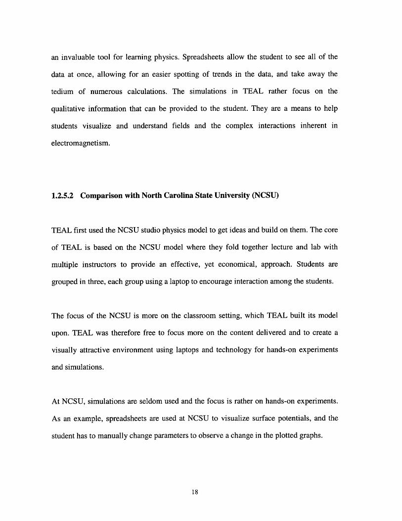
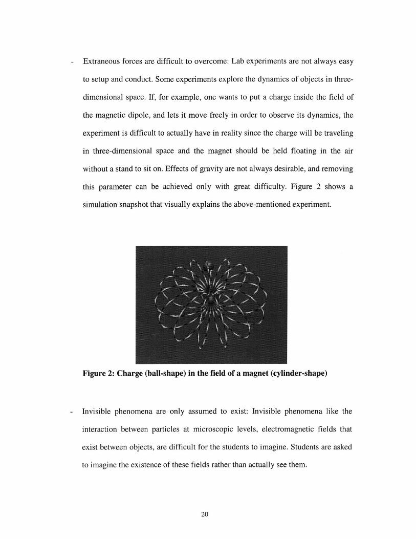
without a stand to sit on. Effects of gravity are not always desirable, and removing
this parameter can be achieved only with great difficulty. Figure 2 shows a
simulation snapshot that visually explains the above-mentioned experiment.
Figure 2: Charge (ball-shape) in the field of a magnet (cylinder-shape)
Invisible phenomena are only assumed to exist: Invisible phenomena like the
interaction between particles at microscopic levels, electromagnetic fields that
exist between objects, are difficult for the students to imagine. Students are asked
to imagine the existence of these fields rather than actually see them.
20

1.3.2 Traditional Teaching and Technology
Traditional teaching in the traditional classroom has made poor use of technology with
only videos and slide shows being the main visually appealing and exciting applications
used. Computer power has been for the most part ignored in teaching, even though it can
provide a way for the student to be more active in the classroom rather than passively
receive the information delivered by the teacher. It can also assist lab experiments in
calculating and plotting parameters such as current and voltage when it is plugged into
the experiment. Simulations are also a powerful tool that the computer can achieve by
providing a quasi real-time depiction of phenomena plus the added details that we are
interested in such as invisible phenomena and microscopic interactions.
1.3.3 Mathematical Difficulties
Lectures give a mathematical explanation
In physics, traditional lectures focus on the mathematics of idealized systems, the
equations that explain the science, and how from derivations of the equations one can
show that the science is correct. By solving a coupled set of equations, for example, we
can see that the trajectory of a projectile is a parabola. How did we learn it? By starting
with the acceleration of the gravity and then integrating twice. If we had a simulation
with the vectors of accelerations and velocities and their sums following the projectile
21
during the motion, we could have seen how these change over time, and how they end up
drawing a parabola.
Similarly, in electromagnetism, mathematical equations tell us that the field existing
between a charge and another will drive motion of these two relative to each other. The
grasp of the meaning of these equations can be obtained by actually seeing two charges in
motion, and observing their behavior. Mathematical equations give us a clear answer that
we can be certain of within the simplifying assumptions of the system they model, but
that does not easily relate to reality. Problem solving focuses on the abstract realm, but
often does not convey concepts in the form of qualitative information.
Mathematical equations are sometimes complex
Solving equations is sometimes complex. Having coupled equations to solve focuses the
student on solving a mathematical problem, and forgetting how to relate back to the
physics concepts that were the primary goal. Concepts are not easy to grasp, and
visualizations, simulations and conceptual questions aid the student in understanding
them. Computer simulations have the potential to expand the range and nature of student
experiences and, if properly designed and used, will expand their understanding of
physics.
22
Chapter 2
Technology Background
A brief introduction to the various technologies used in developing the software is
presented here.
2.1 Java
Java was used for the development of the simulations. It was an attractive solution for its
portability across different platforms and imaging capabilities. It also allows the
development of user interfaces rapidly. Below is a brief description of Java, and a taste of
its benefits and limitations.
Introduced by Sun Microsystems, Java was the first programming language that was not
tied to any particular operating system or microprocessor. Applications written in Java
will run anywhere, eliminating one of the biggest headaches for computer users:
incompatibility between operating system and versions of operating systems. Java started
23
in 1990 when a team of Sun researchers developed technology for the convergence of
digitally controlled consumer devices and computers.
Java is directly derived from C++ and was designed with many goals in mind. Its
designers wanted a new language that was familiar, simple, object-oriented, platform
independent, high-performance, multi-threaded, robust and secure. To this end, a number
of more complicated features of C++ such as pointers, multiple inheritance and operator
overloading were omitted from Java. Java is a language of the 1990's and quickly gained
fame as the language of the Internet. It was recognized that a language for the Internet
would present immense security worries. Users would not want to download executable
programs to their local machines if these routines had the potential to wreck their local
working environments. The creators of Java built into the language mechanisms that
prevent remotely loaded routines from taking control of the machine they run on,
particularly when using Java applets.
2.2 Java Applets
The simulations developed are Java applets that do not present serious security threats
when downloaded from the network and run on the client machine. They are also
relatively small in size, and therefore attractive to be downloaded to the client end.
A Java applet is a Java program that is cross-platform compatible and can be embedded
in the HTML' of a Web page. An applet may be downloaded over a network connection
24
1 Hypertext Markup Language
and run on a local machine via a Java-enabled browser. Web browsers that are equipped
with Java virtual machines can run an applet to perform interactive graphics, games,
calculators, etc. Applets can add sophisticated support for Web pages, far beyond other
programming such as DHTML 2 or JavaScript. Applets provide a means of doing client
side data manipulation under the HTTP3 protocol. Unlike complete applications, applets
cannot be executed directly from the operating system. A well-designed applet can be
invoked from many different applications.
Applets differ from applications in that they are more secure -- they cannot access certain
resources on the connection to the computer from which the applet was sent (local
computer, such as hard drives, modems, and printers). Applets can in some cases slow
page loading to a crawl, and just plain crash non-compatible browsers.
2.3 Java3D
A number of simulations were developed in three dimensions for the greater sense of
reality they would present, and the extra information they would contain and the need for
students to look at the objects and field lines from different angles. Plane cuts could have
allowed these different two-dimensional views, but one could not, in that fashion, provide
a complete picture of the other planes. Java presented an easy solution through the use of
the Java3D package.
25
2 Dynamic HTML3 Hypertext Transfer Protocol
As a part of the Java Mediaproduct family, the Java3D Application Programming
Interface (API) is used for writing stand-alone three-dimensional graphics applications or
Web-based three-dimensional (3D) applets. It gives developers high-level constructs for
creating and manipulating 3D geometry and tools for constructing the structures used in
rendering that geometry. With Java3D API constructs, application developers can
describe very large virtual worlds, which, in turn, are efficiently rendered by the Java3D
API.
The Java3D API specification is the result of a joint collaboration between Silicon
Graphics, Inc., Intel Corporation, Apple Computer, Inc., and Sun Microsystems, Inc. All
had advanced, retained mode APIs under active internal development, and were looking
at developing a single, compatible, cross-platform API using Java technology.
The Java3D API draws its ideas from the considerable expertise of the participating
companies, from existing graphics APIs, and from new technologies. The Java3D API's
low-level graphics constructs synthesize the best ideas found in low-level APIs such as
Direct3D API's (http://www.direct3d.net/), OpenGL (http://www.opengl.org/),
QuickDraw3D (http://www.apple.com/guicktime/, and XGL (http://www.xglspec.org).
Similarly, the Java3D API's higher-level constructs leverage the best ideas found in
several modern scene graph-based systems. This API also introduces some concepts not
commonly considered part of the graphics environment, such as three-dimensional spatial
sound to provide a more immersing experience for the user.
26
2.4 XML
The simulations developed are all part of one software framework. The creation of a
simulation starts with reading a configuration file, written in XML (Extensible Markup
Language). XML (http://www.w3.org/XMIU) was chosen because it is human readable,
easy to write, and can present the non-programmer with an attractive way to develop a
new simulation by simply looking at an example. Further explanation of how XML was
incorporated in the framework can be found in sections 4.1.4 and 4.2.1. In this section,
we present an overview of XML.
Extensible Markup Language (XML for short) is a new language derived from Standard
Generalized Markup Language (SGML) designed to make information self-describing.
This simple sounding change in how computers communicate and exchange data has the
potential to extend the Internet beyond information delivery to many other kinds of
human activity. Since XML's specification was completed in the early 1998 by the World
Wide Web Consortium (W3C), the standard has spread through science and into
industries ranging from manufacturing to medicine. This enthusiastic response is fueled
by a hope that XML will solve one of the Web's biggest problems: although every kind
of information is available online it can be extremely difficult to find the information one
needs. The problem arises from the nature of the Web's main language, HTML
(shorthand for Hyper Text Markup Language). Although HTML is the most successful
electronic publishing language ever invented, it is superficial. In essence it describes how
a Web browser should arrange text, images and widgets on a page. HTML's concern with
appearance makes it a relatively simple language to learn, but this simplicity also has its
costs. XML makes it possible, despite the use of incompatible computer systems, to
27
create a data format that all can read and write. Unlike most computer data formats, XML
markup also makes sense to humans, because it contains nothing more than ordinary text.
The unifying power of XML comes from a few well-chosen rules. One is that tags almost
always come in pairs. Like parentheses, they surround the text to which they apply. And
like quotation marks, tag pairs can be nested inside one another to multiple levels. The
nesting rule automatically forces certain simplicity on every XML document, which takes
the structure of a tree. Each element in the document represents a parent, child or sibling
of another element; relationships are unambiguous. Trees cannot represent every kind of
information, but they can represent most kinds which we need computers to understand.
28
Chapter 3
Simulations
3.1 Research Goals
The simulations that were designed as part of TEAL were created in order to make the
task of learning more interesting and more effective. Students are used to sitting in a
traditional classroom and listening to the explanation of the teacher, with only occasional
questions from the teacher or the student that provide interactivity during class time.
Laboratory experiments are a way to make the students more active. These hands-on
experiments help the student get a better feel for the abstract explanations given in class
by providing actual physical components to the students. Nevertheless, not all
experiments are possible, be it simply because it is very hard to get rid of some
surrounding phenomena such as gravity, or because some phenomena such as field lines
in electromagnetism or forces in mechanics are invisible.
On another hand, traditional teaching has mainly focused on problem solving tasks and
"plug-and-chug" exercises. In our work, we focus on improving students' conceptual
understanding, and present qualitative information to students rather than quantitative
29
problems. Qualitative information can be presented through visualizations and
simulations.
The simulations were designed to make learning more appealing. They relate to real-life
situations by having the objects' properties in the simulations similar to the ones in real
electromagnetic objects. The simulations all have the same look-and-feel in order for the
student to be able to use the same simulations' environment throughout the semester. We
explore below the research goals in detail.
3.1.1 Complement Laboratory Experiments
Traditional science lectures present the concepts to the students, and explain difficult
ones through equations that quantify those concepts. Laboratory experiments give the
student a more hands-on experience with the concepts learnt in class. Nevertheless, not
all experiments are possible to conduct. Gravity for example is a factor that cannot be
practically eliminated; some explanations of concepts need to remove this component in
order to be easily understood.
Some other phenomena, such as field lines in electromagnetism, forces in mechanics and
chemical reactions at the molecular level, are invisible. By designing simulations, the
limitations of the desktop experiments can be overcome, whereby constraining factors
can be eliminated by one click of the mouse, and invisible phenomena can be easily
visualized through line drawings, vector representations and visual illustrations.
30
3.1.2 Improve Conceptual Understanding
We focus on improving the conceptual understanding of the students by:
- Presenting visual understanding of interactions between objects that are not
evident from equations: The simulations have the ability to show the students the
interactions among objects and the unseen phenomena. Equations explain the
concepts but do not make evident phenomena such as the actual charge
distributions, field lines, equipotentials and dynamics. Once the students visualize
these aspects, they can more easily understand the complexity of the equations
presented in class.
- Interactively demonstrating concepts: All the simulations should be interactive.
This makes the students more interested in spending time changing parameters in
the simulation and observing the corresponding behavior. Moreover, the students
are given control over the parameters of the physical objects. They can also
choose to show or hide invisible phenomena such as field lines, or choose the
visualization that is most suitable for the simulation such as the texture for the
field lines. By texture, we mean the way we draw the field lines: they can either
be continuous lines, made up of vectors with direction and intensity, filling the
whole surrounding space, or drawn at specified points only.
31
- Asking conceptual questions: While the student interacts with the simulations we
display conceptual questions related to them. This makes sure the student
comprehends the theory that the simulation is trying to explain. We will explore
this area more in section 5.5.
3.1.3 Provide a Comfortable Learning Environment
Another goal of the simulations is to provide an easy environment for students to deal
with. The students are naturally driven to spend more time interacting with the
simulations until they can relate the simulated objects and environment to reality.
Simulation objects have the same properties as their physical counterparts:
Electromagnetic objects have sizes, magnetic moments, charges, mass, current, etc....
The students therefore deal with parameters they are used to in desktop experiments, but
with the added facility that these parameters can be changed very easily. By typing in a
new value, or just by moving the pointer of a slider, one can change any of the
parameters.
Students deal with a common user interface: The simulations follow a common graphical
user interface (GUI) in order for the student to be acquainted with the environment
instead of coping with a new environment for each animation.
32
3.2 Simulations in Physics Instruction
In this section, we present the work done by previous and concurrent physics teaching
efforts, and then present our work followed by examples and the challenges that we
faced. A clarification is needed here to distinguish between simulation and visualization.
Simulations are applications that one can interact with. We mention a few examples such
as changing the simulation's parameters, watching it from different angles, grabbing
objects and changing their locations. In contrast, visualizations are just static images and
videos that the user cannot modify.
3.2.1 Previous Work
Previous efforts to create physics simulations for educational purposes have been
conducted at several universities. We split previous simulations into static and dynamic
ones.
Static simulations are simulations where objects do not have dynamics equations that
drive them. Dragging objects from one position to another is their sole displacement.
Colorado University and Georgia Tech have worked in this area and their simulations
were interactive. One can change the parameters of the E&M objects and drag them
around. These simulations are attractive and have good functionality but they are limited
by their intrinsic static nature. Below are two snapshots of their work. Figure 3 shows a
positive charge and a negative one. The smaller circles are points where the electric field
33
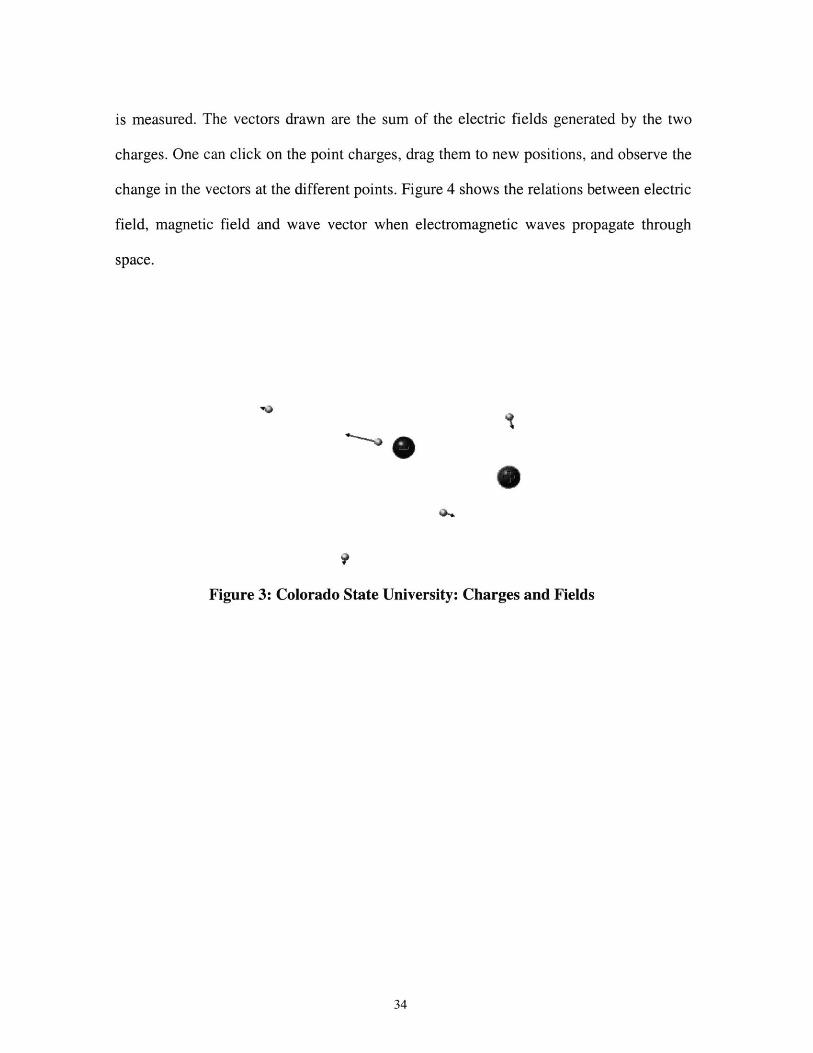
is measured. The vectors drawn are the sum of the electric fields generated by the two
charges. One can click on the point charges, drag them to new positions, and observe the
change in the vectors at the different points. Figure 4 shows the relations between electric
field, magnetic field and wave vector when electromagnetic waves propagate through
space.
Figure 3: Colorado State University: Charges and Fields
34
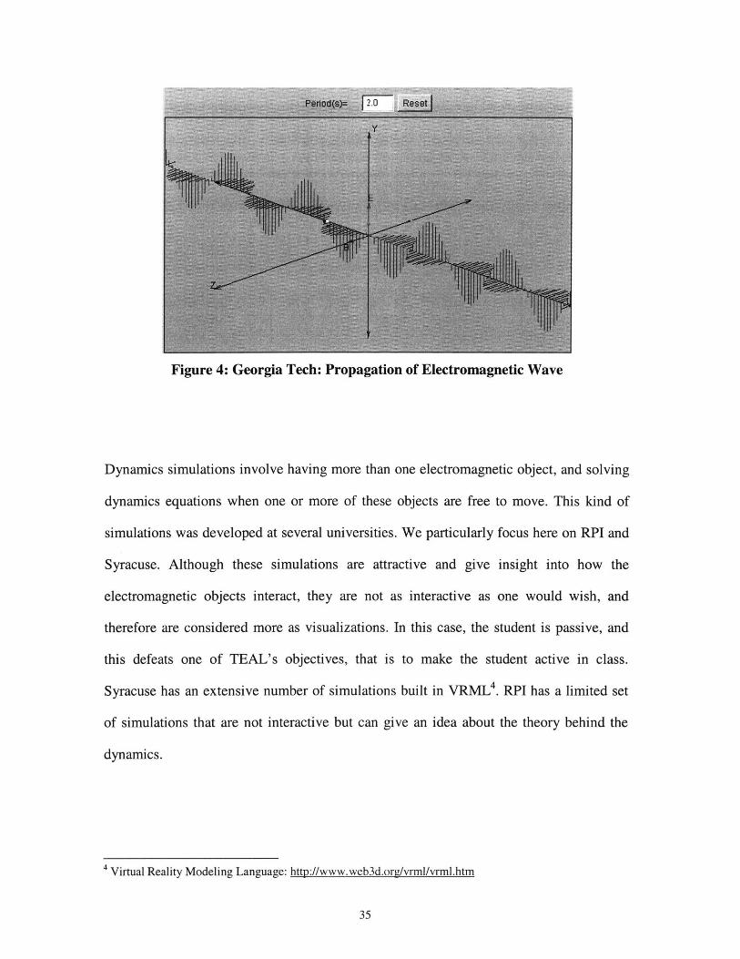
Figure 4: Georgia Tech: Propagation of Electromagnetic Wave
Dynamics simulations involve having more than one electromagnetic object, and solving
dynamics equations when one or more of these objects are free to move. This kind of
simulations was developed at several universities. We particularly focus here on RPI and
Syracuse. Although these simulations are attractive and give insight into how the
electromagnetic objects interact, they are not as interactive as one would wish, and
therefore are considered more as visualizations. In this case, the student is passive, and
this defeats one of TEAL's objectives, that is to make the student active in class.
Syracuse has an extensive number of simulations built in VRML4. RPI has a limited set
of simulations that are not interactive but can give an idea about the theory behind the
dynamics.
4 Virtual Reality Modeling Language: http://www.web3d.org/vrml/vrml.htm
35
At these universities and others that we did not mention, the simulations did not cover the
entire curriculum of the class. There were only few simulations that the teachers found
useful or practical to have. They were therefore not exhaustive of the syllabus followed in
class.
One major issue in electromagnetism is the field lines drawn around and between
electromagnetic objects and how the drawing is done. Each of the previous ventures
focused on one texture used to represent fields that was followed in all the simulations. In
this context, texture refers to the way field lines are to be represented (dotted lines,
vectors at different points of the line, lines filling the whole surrounding space or just a
few lines drawn). This is an expected behavior when the same teacher is teaching the
class, but different teachers have different preferences for representing field lines. Some
prefer dotted field lines, others ones formed of small vectors, and others prefer the usage
of continuous lines. These textures give different viewpoints to the fields. They are all
useful, but some are more informative than others, depending on the simulation. We will
show in our simulations how different simulations require different textures to best
illustrate the key concepts students need to learn.
3.2.2 Simulations Achievements
The simulations that we designed followed the curriculum of the electromagnetism class
taught at MIT.
36
These simulations were designed in two-dimensional and three-dimensional space
according to the needs of each simulation. If a two-dimensional simulation was
sufficient to explain a certain concept, then we did not bother to go to the third
dimension, therefore sparing the student unnecessary complexity. This brought an
added value to previously designed simulations where only two-dimensional
simulations existed. We used Java3D to have good graphics resolution and speed
of simulation.
Each simulation explained a new concept or law (Faraday's Law, Coulomb's
Law, Lorentz's equations, Maxwell's equations, etc...) so that the entire syllabus
was covered, in contrast to other physics efforts at other universities where only a
limited number of simulations were created.
Each simulation shows field lines the way we judged most useful to that particular
simulation. Some are drawn as dotted lines; others are formed of vectors at
different locations along the line. For the three-dimensional simulations, we draw
a few field lines surrounding the E&M objects. These simulations would not be
very informative if field lines were drawn at every point in the surrounding space
because that would hinder visualizing the objects themselves, even if the field
lines were made semi-transparent. Instead, a few lines are enough for three-
dimensional simulations. We discuss this further below.
All simulations are interactive in the sense that all the parameters of the
simulations can be changed.
37
An easy look-an-feel made it simple for students to have everything they were
able to manipulate easily accessible. For example, students can easily alter the
charge of a point, whether to display field lines, change grid spacing, etc.
Numerical methods for integration of differential equations were properly chosen
in order to accurately draw the field lines and calculate the objects' dynamics.
Different integration schemes were used, and one could choose between Euler,
Runge Kutta and stepped Runge Kutta. Euler's method is the fastest but least
accurate. When one uses Runge Kutta, further details can be visualized and more
accurate calculations result. In particular, when we want the magnetic field lines
to follow their loop path and close down on themselves, Euler is not guaranteed to
achieve that, and instead the simulated field lines would diverge and go to
infinity.
Sound was added to some simulations where necessary. For example, a magnet
falling inside a ring of current had attractive graphics (see Figure 7) and an
ammeter to measure the current inside the ring, but a more impressive way to do it
was to add sound that was proportional to the square of the current in the ring.
This feature does not exist in previous or concurrent efforts in physics
simulations.
Line Integral Convolution
38
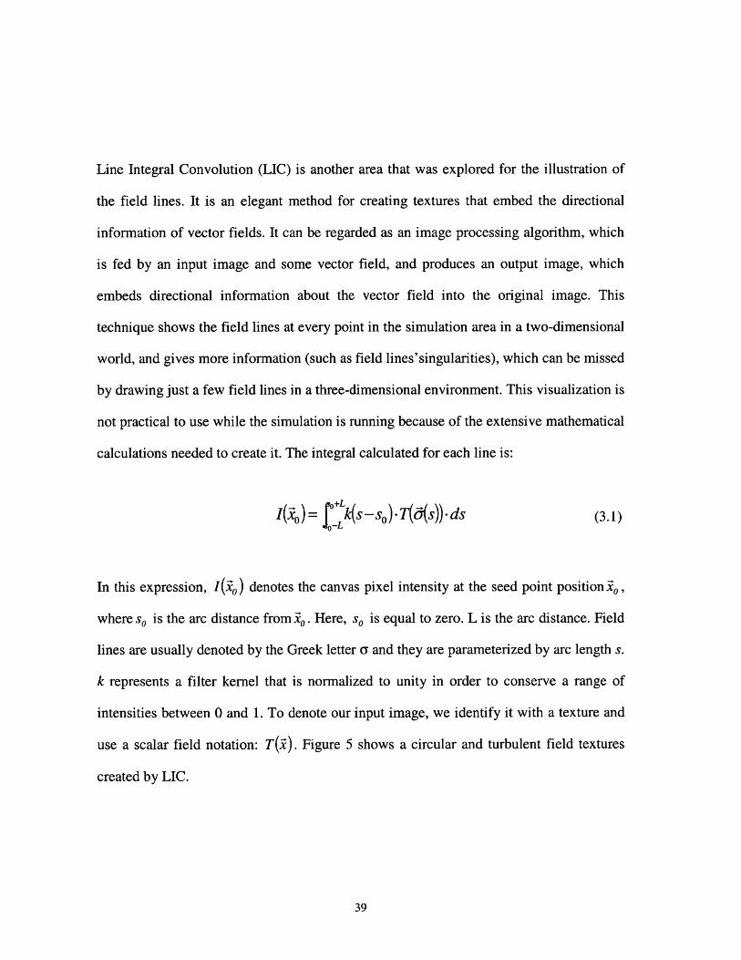
Line Integral Convolution (LIC) is another area that was explored for the illustration of
the field lines. It is an elegant method for creating textures that embed the directional
information of vector fields. It can be regarded as an image processing algorithm, which
is fed by an input image and some vector field, and produces an output image, which
embeds directional information about the vector field into the original image. This
technique shows the field lines at every point in the simulation area in a two-dimensional
world, and gives more information (such as field lines'singularities), which can be missed
by drawing just a few field lines in a three-dimensional environment. This visualization is
not practical to use while the simulation is running because of the extensive mathematical
calculations needed to create it. The integral calculated for each line is:
I(O) kgs - so) -T(6 s)) -ds (3.1)
In this expression, I(i,) denotes the canvas pixel intensity at the seed point positionio,
where so is the arc distance fromio. Here, so is equal to zero. L is the arc distance. Field
lines are usually denoted by the Greek letter a and they are parameterized by arc length s.
k represents a filter kernel that is normalized to unity in order to conserve a range of
intensities between 0 and 1. To denote our input image, we identify it with a texture and
use a scalar field notation: T(i). Figure 5 shows a circular and turbulent field textures
created by LIC.
39
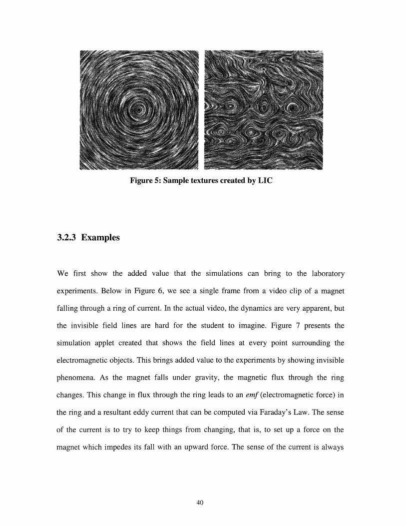
Figure 5: Sample textures created by LIC
3.2.3 Examples
We first show the added value that the simulations can bring to the laboratory
experiments. Below in Figure 6, we see a single frame from a video clip of a magnet
falling through a ring of current. In the actual video, the dynamics are very apparent, but
the invisible field lines are hard for the student to imagine. Figure 7 presents the
simulation applet created that shows the field lines at every point surrounding the
electromagnetic objects. This brings added value to the experiments by showing invisible
phenomena. As the magnet falls under gravity, the magnetic flux through the ring
changes. This change in flux through the ring leads to an emf (electromagnetic force) in
the ring and a resultant eddy current that can be computed via Faraday's Law. The sense
of the current is to try to keep things from changing, that is, to set up a force on the
magnet which impedes its fall with an upward force. The sense of the current is always
40
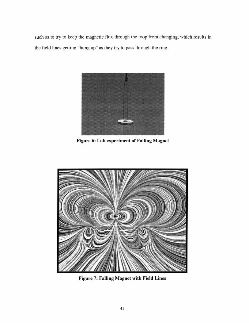
such as to try to keep the magnetic flux through the loop from changing, which results in
the field lines getting "hung up" as they try to pass through the ring.
Figure 6: Lab experiment of Falling Magnet
Figure 7: Falling Magnet with Field Lines
41
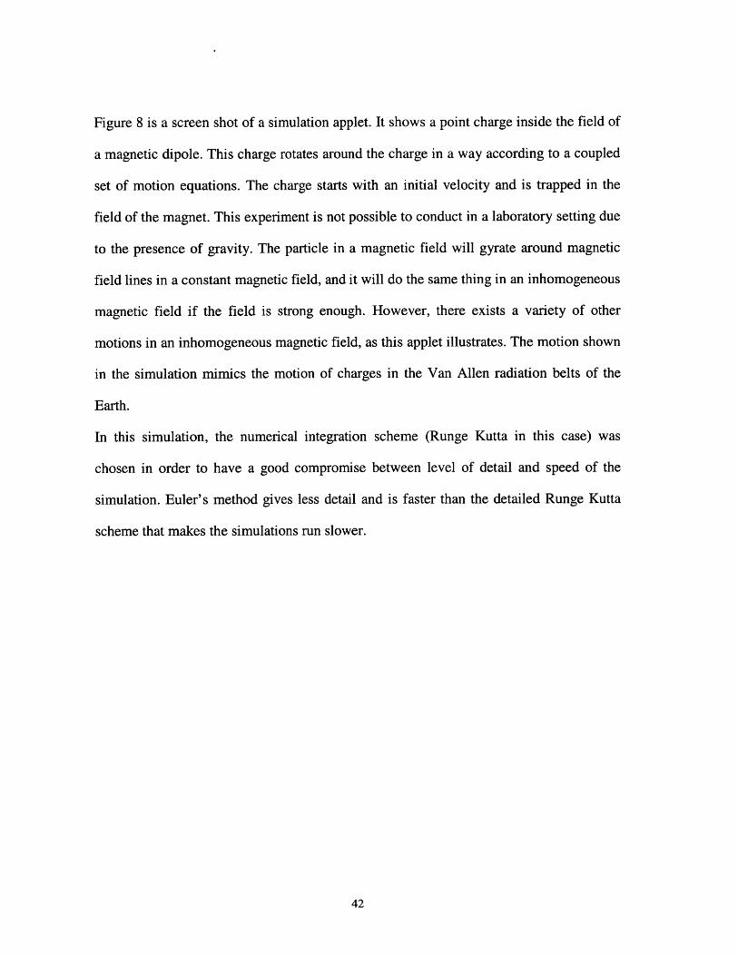
Figure 8 is a screen shot of a simulation applet. It shows a point charge inside the field of
a magnetic dipole. This charge rotates around the charge in a way according to a coupled
set of motion equations. The charge starts with an initial velocity and is trapped in the
field of the magnet. This experiment is not possible to conduct in a laboratory setting due
to the presence of gravity. The particle in a magnetic field will gyrate around magnetic
field lines in a constant magnetic field, and it will do the same thing in an inhomogeneous
magnetic field if the field is strong enough. However, there exists a variety of other
motions in an inhomogeneous magnetic field, as this applet illustrates. The motion shown
in the simulation mimics the motion of charges in the Van Allen radiation belts of the
Earth.
In this simulation, the numerical integration scheme (Runge Kutta in this case) was
chosen in order to have a good compromise between level of detail and speed of the
simulation. Euler's method gives less detail and is faster than the detailed Runge Kutta
scheme that makes the simulations run slower.
42

Figure 8: Point Charge and Magnet
In Figure 9, we see a complete example of how the textures can be drawn. We see
equipotentials (lines formed of small vectors) that were obtained by clicking on any point
on these lines. The arrows on these lines show the vectors that form these lines. The
direction of the vectors is also very important to indicate where these field lines
originated at, and which direction they are pointing to.
43
Applet started,
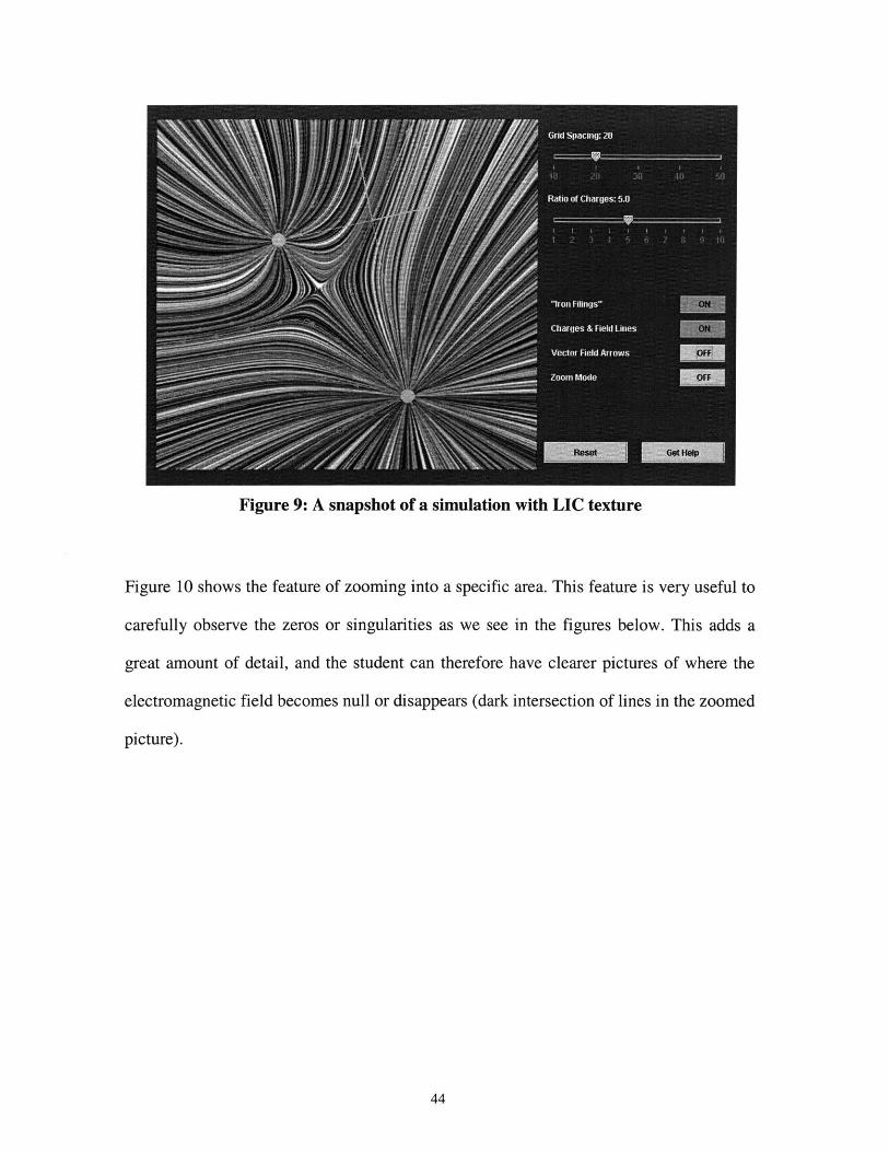
Figure 9: A snapshot of a simulation with LIC texture
Figure 10 shows the feature of zooming into a specific area. This feature is very useful to
carefully observe the zeros or singularities as we see in the figures below. This adds a
great amount of detail, and the student can therefore have clearer pictures of where the
electromagnetic field becomes null or disappears (dark intersection of lines in the zoomed
picture).
44
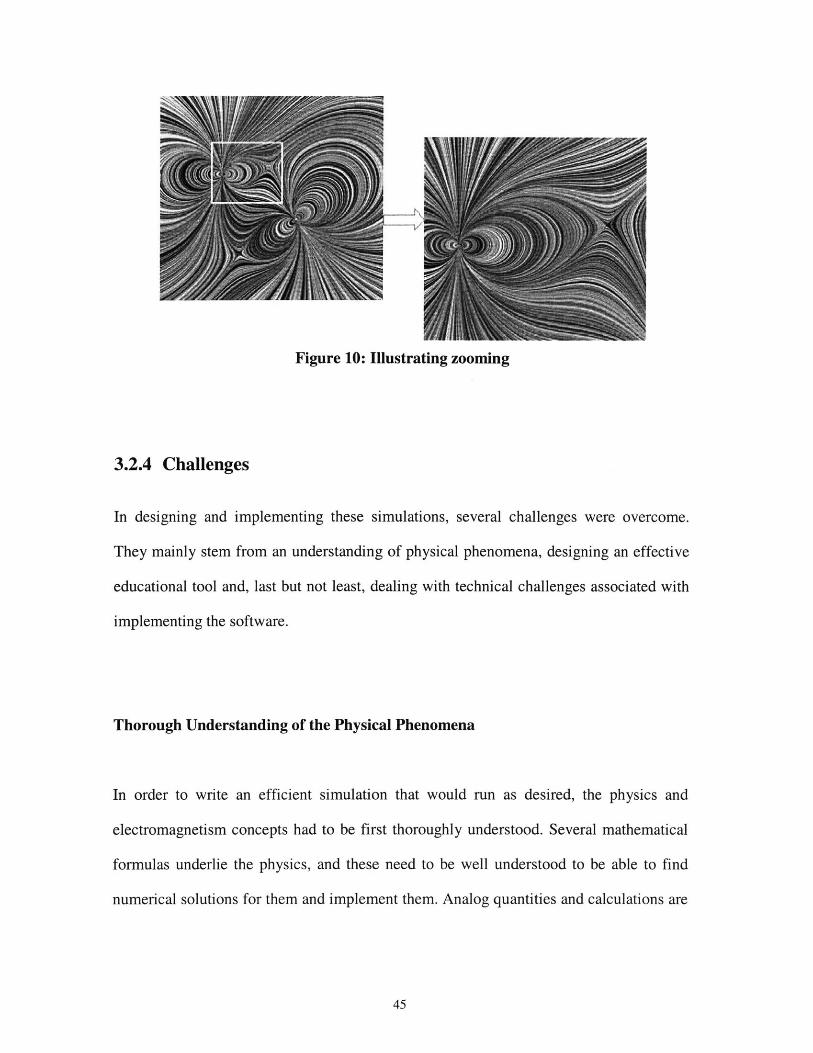
Figure 10: Illustrating zooming
3.2.4 Challenges
In designing and implementing these simulations, several challenges were overcome.
They mainly stem from an understanding of physical phenomena, designing an effective
educational tool and, last but not least, dealing with technical challenges associated with
implementing the software.
Thorough Understanding of the Physical Phenomena
In order to write an efficient simulation that would run as desired, the physics and
electromagnetism concepts had to be first thoroughly understood. Several mathematical
formulas underlie the physics, and these need to be well understood to be able to find
numerical solutions for them and implement them. Analog quantities and calculations are
45
to be quantized and digitized to have accurate numerical solutions to the underlying
equations.
Educational Effectiveness
We started with goals in mind of stimulating the student's interest and creating a tool that
brings proper understanding of the concepts. We were therefore bound to design
attractive simulations that we refined according to a few rounds of student feedback. We
took into account their comments, observed their behavior, and were able to develop an
effective tool that would offer an easy-to-use interface, with defined separations between
controls of E&M objects and the parameters of the simulation. For example, at first,
students wanted to be able to add point charges during the simulation. We therefore
added that functionality to the framework. Another example that is relevant to the GUI is
the ease of use. Students had difficulty finding the appropriate buttons and sliders. We
agreed therefore on having all the simulation controls on the right side of the applet
window. After this change, students did not complain and were more comfortable with
the simulations.
The number of parameters that we can let the student change are numerous;
consequently, a careful choice of parameters was studied to bring the students the needed
educational value: a balance was struck between the number of controls, their
functionality, and the parameters that play a role in understanding the concept presented.
46
Figure 9 shows us a well-balanced graphical user interface that most of the students felt
comfortable dealing with.
Technical Challenges
A great amount of know-how of Java3D helped us make the most out of three-
dimensional vectors in the VecMath package, which is incorporated in the Java3D
package. The Sound3D package was able to provide a realistic three-dimensional
surrounding sound to the student.
Earlier versions of the software were implemented using the classic AWT library of Java.
This library was not well suited for graphics, especially when dealing with animations.
The Swing package used in subsequent versions provided us with built-in buffered
images that did not have any flickering.
The speed of the simulations was a challenge since we were dealing with students who
had different computer processor speeds. Therefore, the code was optimized to minimize
the number of calculations that were required in order to have approximately the same
animation speed on all the computers. The agreed-upon speed was chosen to keep the
students' interest high.
Furthermore, the code structure was refined over time to make new simulations easy to
develop by people that would join our group, and who were not involved in the cycles we
47
went through. In addition, the maintenance of the software was not costly, due to a good
design from the start. Changing an integration scheme for the entire set of simulations
would not have to be fixed in all the simulations for example, but instead in one place
only. This brings us to the next chapter that explains about the structure of the software
that made all this possible, and that made the creation of new simulations an easy task for
non-programmers to achieve.
3.3 Value of Accomplishments
The simulations that were part of the work in TEAL had many benefits educationally and
on the software practice point of view.
3.3.1 Students' Feedback
An assessment of TEAL's benefits was conducted by Yehudit Dori [11], and we mention
here some of the feedback from the students.
Student A: "This is my third time around trying to take 8.02 and I will honestly say that
in order for me to grasp the concepts of 8.02 1 NEEDED to "see" them in action as
clearly as possible. However, I can't just understand it by following the steps of the
protocol, anyone can do that, the oral explanations of what was going on helped put it all
together in my mind."
48

Student B (Fall 2001): "Desktop experiments help to really grasp the conceptual
background of various problems while integrating calculations and quantitative analysis.
Visualizations and conceptual questions also help to explain what is really happening
behind all the numbers."
In Fall 2001, the end-term survey the question had the question: "Would you recommend
this course to a fellow student?" and the answers are listed in Table 1. The majority of
students indicated they would recommend the TEAL course to fellow students without
any reservation.
Table 1: Student Recommendations
Answer Type Frequency Examples
Yes 45%
Yes, with 26% Yes. The interactivity makes it much moreexplanation interesting and easy to learn when compared
to traditional lecture style. Definitely. Myimpression of 8.02T is that it conveys theconcepts of electricity and magnetism in amuch more visual and hands-on way than thestandard 8.02 class.
Maybe, yes but... 22% I would recommend it to any student who is notplanning on majoring in course 8, or whodoesn't need to take more advanced physicsclasses. I feel like 8.02T was a good class fornon-physics majors because it was interesting,and the pace was good.
No 4%
No, with explanation 3% No. I was looking for a more complicatedphysics class. I wanted more conceptual work,and in-depth approach.
49
3.3.2 Students' Performance
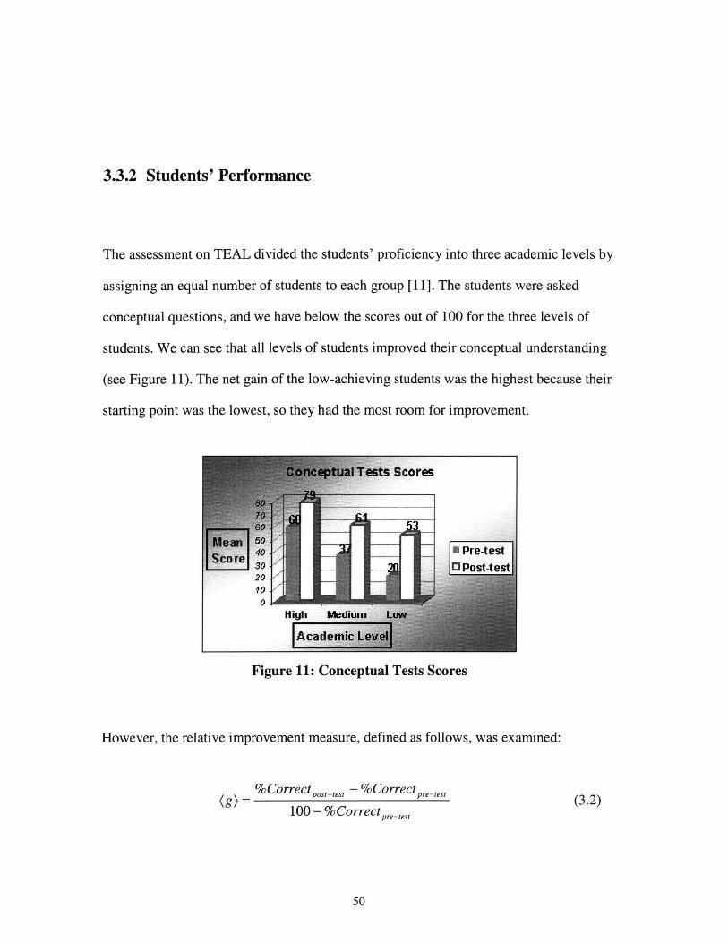
The assessment on TEAL divided the students' proficiency into three academic levels by
assigning an equal number of students to each group [11]. The students were asked
conceptual questions, and we have below the scores out of 100 for the three levels of
students. We can see that all levels of students improved their conceptual understanding
(see Figure 11). The net gain of the low-achieving students was the highest because their
starting point was the lowest, so they had the most room for improvement.
rests Scores
I~10Pre-test
High Medium LA aw
F Academic LevelTtSr
Figure 11: Conceptual Tests Scores
However, the relative improvement measure, defined as follows, was examined:
(g) =%Correctpost-test -%Correctpre-test
100 - %Correctpretest(3.2)
50
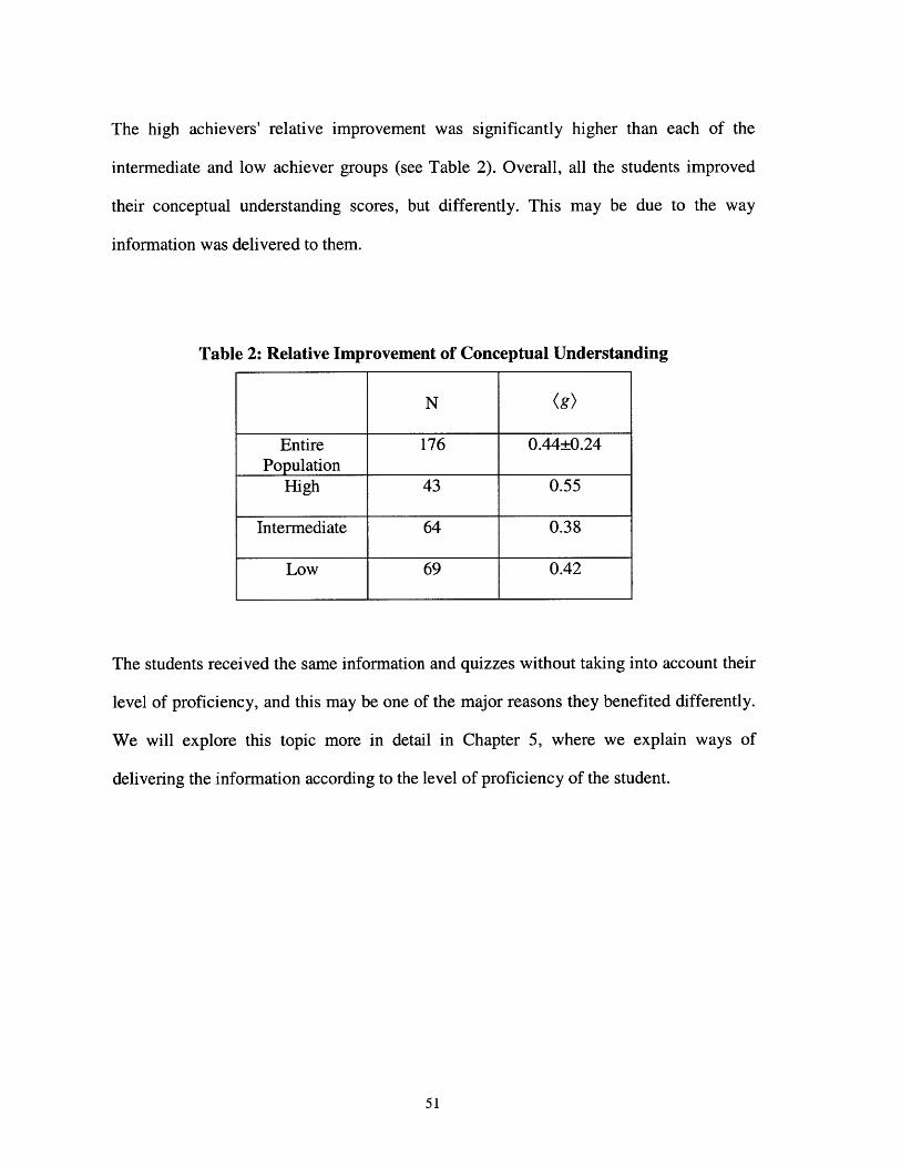
The high achievers' relative improvement was significantly higher than each of the
intermediate and low achiever groups (see Table 2). Overall, all the students improved
their conceptual understanding scores, but differently. This may be due to the way
information was delivered to them.
Table 2: Relative Improvement of Conceptual Understanding
N (g)
Entire 176 0.44±0.24Population
High 43 0.55
Intermediate 64 0.38
Low 69 0.42
The students received the same information and quizzes without taking into account their
level of proficiency, and this may be one of the major reasons they benefited differently.
We will explore this topic more in detail in Chapter 5, where we explain ways of
delivering the information according to the level of proficiency of the student.
51
Chapter 4
Software Framework
4.1.1 Framework Motivation
TEAL requires a large number of computer simulations that collectively span the
curriculum. Nevertheless, this curriculum may change over time. We cannot guarantee
that the set of simulations that we create at the present time will still be useful in a few
years. We therefore had to come up with a way to make creating new simulations an easy
task.
Furthermore, a number of teachers will teach the class in subsequent semesters, and each
has preferences for which simulations to use or not, modify existing ones, or create new
ones that they feel are useful.
52
These reasons were the drivers to come up with a set of requirements while designing our
simulations and the software framework that these simulations would be part of. The
prominent requirements were:
- Interactive animations and configurable parameters: The student should be able to
dynamically alter the state of the different electromagnetic objects in the
simulation and even add and remove electromagnetic objects dynamically.
- Modular architecture in order to make it possible for developers to reuse software
components in multiple simulations. Different modules communicate with each
other through well-defined interfaces.
- Consistent and extensible method for incorporating the physics into the
simulations in order for new developers to be able to add new features they find
necessary. If the existing components do not provide the required functionality,
new implementations can be written and plugged in, as long as they conform to
the interface used to communicate with other components.
- Easy and convenient API to manage objects that have to be rendered on the
screen.
- Virtual instrumentation for drawing graphs representing the variation of different
parameters of the simulation. This requirement was set in order to simulate the
53
desktop experiments and to have the same measurements available that the
student is used to when doing hands-on experiments.
4.1.2 Important Components/Classes and Interfaces
The following are the main components in any simulation.
EMObject
All the physical and electromagnetic properties of objects like PointCharge,
ElectricDipole, etc... are abstracted into a base class called EMObject. The different
electromagnetic objects are represented by concrete implementations of this base class.
EMObjectHandler
EMObjectHandler is a class used to model the physical and electromagnetic behavior of
an electromagnetic object. Different EMObjectHandlers are developed for each
electromagnetic object each modeling the respective behavior of their corresponding
physical object. In its simplest form, the EMObjectHandler for a PointCharge models the
dynamics of a PointCharge by calculating the force acting on the PointCharge using the
equation:
F = q (E + v x B) (3.2)
54
Where: F is the Lorentz force exerted on a test point charge (in Newtons), q is the charge
(in Coulombs), E is the electric field (in Newtons/coulombs), v is the velocity (in m/sec),
and B is the magnetic field (in Newtons/Amp).
In short, EMObjectHandler encapsulates the electromagnetic behavior of an EMObject.
There could be various reasons for developing different EMObjectHandlers for the same
EMObject. For example, if only one degree of freedom is active for a simulation, we
want to use a handler that takes this into account instead of using a generic three degrees
of freedom handler, for performance reasons. Different simulations may emphasize
different physical principles, making it necessary to associate a different behavior to the
EMObject. This is achieved by using a different EMObjectHandler for the EMObject in
different simulations.
Force Model
This is an interface that encapsulates the necessary properties of physical forces like
friction, gravity, etc... By creating new implementations of this interface, different forces
can be simulated.
ImpulseModel
55
All the necessary properties of any object, which exerts an impulse on the EMObjects in
the simulation, are encapsulated in this interface. A simple example is the boundary of
the simulation area. Whenever an EMObject hits the boundary, it gets reflected back so
that the object never leaves the simulation area. This is very easily modeled as an impulse
being exerted on the EMObject whenever it reaches the boundary. Another place where
impulses could be used is when there are collisions between EMObjects.
SimulationModel
This is the central control of the simulation. All the EMObjects that are added to the
simulation register themselves with the SimulationModel. For every simulation step, the
simulation model updates the different EMObjects accordingly.
Drawable
This is an interface to be implemented by all objects that have to be rendered on the
screen. Whenever a new object that has to be rendered on the screen is added to the
simulation, if it implements this interface, it is registered with the simulation to be
rendered at the end of every simulation step.
FieldLine
56
Electromagnetic field lines are an excellent way to depict the variation of electric and
magnetic fields as the simulation progresses. Every EMObject for which the field lines
have to be drawn has a FieldLine object associated with it. Points relative to the
EMObject can be specified through which the field lines will be drawn. Since the field
lines have to be rendered as part of the simulation, FieldLine implements the Drawable
interface.
SimulationApplet
This is the class that actually starts the simulation and acts as a container for the
simulation. This class features a thread that is used to control the progress of the
simulation. This thread is used to trigger each subsequent step of the simulation.
SimulationPanel
This is the panel where the entire simulation-related rendering occurs. This panel
maintains a list of all the objects that need to be rendered onto the screen. At the end of
every simulation step, all these objects are redrawn on the screen. This object is also in
charge of generating and propagating events at the end of every simulation cycle. Objects
interested in these events must register themselves with the SimulationPanel.
57
GraphPanel
This class acts as a panel for the different graphs to be drawn. This is also the panel
where the actual graphs are displayed. Different graphs that have to be displayed register
themselves with the GraphPanel. After every simulation cycle, all the graphs are updated,
keeping them up-to-date with the simulation.
Graph
This class encapsulates the different properties of a graph. It provides the GraphPanel
with points through which the graph are to be drawn.
SidePanel
Different simulations may have different GUI requirements. For example, some
simulations may want to display the constantly varying parameter values for the different
EMObjects. Other simulations may want to plot and display different graphs relevant to
the simulation or add some controls (example: buttons to add and remove EMObjects).
The SidePanel acts as a container for all the simulation-specific GUI components.
ConfigurationFile
58
The configuration file is an XML file that contains information regarding the simulation
setup and initialization. At the start of a simulation, this file is parsed and the simulation
environment is setup and initialized with default objects, as specified in the configuration
file.
Factory Classes
Factory classes are used to parse the XML configuration file and then create simulation
objects according to the properties read from the configuration file. Every simulation
object whose properties can be set in the XML file induces the creation of a Factory class
first, which then will create the appropriate object. Some of the important factory classes
used are listed here.
- SimulationFactory: This class is responsible for reading the simulation's
configuration file and then setting up the simulation. It is also responsible for
initializing the simulation with parameters read from the configuration field. It
uses various other helper classes to assist in the process.
- EMObjectFactory: This class is used by the SimulationFactory to create
EMObjects that will be added to the simulation. Some of the other tasks that are
performed by this class are: initializing the created EMObjects with default values
read from the configuration file; setting the EMObjectHandler for the EMObject;
59
and setting the FieldLines for the EMObject created. New EMObjectFactories can
be easily developed to have custom creation of EMObjects.
- FieldLinesFactory: This class is used by the EMObjectFactory to set the field
lines that have to be drawn for the EMObjects created by the EMObjectFactory.
4.1.3 Simulation Tasks
In this section, we explain the creation of EMObjects, the rendering of different objects
on the screen and how these processes fit together.
EMObjects Creation
The creation of new EMObjects is handled by the EMObjectFactories. These factories
are created during the setup of the simulation. After these factories are created, they are
registered with the SimulationModel for later use in the simulation. One can create new
EMObjects either at initialization or dynamically during the simulation. In the first case,
the XML file contains the information about the EMObject to be created. In the latter
case, the user is prompted to enter values like mass, velocity and physical properties
before the object is added to the simulation.
Rendering of Objects
60
SimulationPanel is the area where the entire simulation-related rendering occurs. The
objects that are to be rendered implement the Drawable interface. The objects know how
to render themselves on the screen. The SimulationPanel maintains a list of objects that
are to be rendered, so when a new object which implements the Drawable interface is
added to the simulation, it is registered with SimulationPanel, and the SimulationPanel
renders this object on the screen.
Drawing Graphs
GraphPanel is the region where all the graphs for the simulation are drawn. Every
simulation that wants to display graphs should have the GraphPanel as one of its
components. Individual graphs can then register themselves with the GraphPanel.
Simulation Physics
The physics of the simulation are separate from other aspects of the simulation. The
SimulationModel achieves this goal by having all the EMObjects to be simulated
registered with the SimulationModel. At every simulation step, the SimulationModel
computes the next state for all the registered EMObjects.
The simulations are mainly solvers for the differential equations that model the
underlying physics. Depending on the complexity of the equations and the
61
interdependence of the properties of different EMObjects, it may or may not be possible
to dynamically add or remove EMObjects to and from the simulation. As an example,
consider the interaction of point charges. Their behavior is purely a function of the total
electric field due to all the EMObjects. The point charge only needs to know the
ElectricField contribution of other EMObjects. Hence, in this simulation it is possible to
add and remove point charges dynamically. In contrast, consider the interaction of two
electric dipoles. To solve the equations of motion, we have chosen to rely on the
conservation of linear and angular momentum, which very closely couples the two
electric dipoles together. The moment a new electric dipole is added to the simulation, the
equations to be solved using this approach change drastically, making it impossible to
add and remove EMObjects dynamically unless certain approximations are made. There
are therefore two types of SimulationModels: one that allows us to add and remove
EMObjects dynamically, and one that does not let us change the number of EMObjects in
the simulation.
4.1.4 Simulation Setup
The first step in any of the simulations is the setup according to the configuration file (see
Figure 12). First, the SimulationPanel class for the simulation is read from the
configuration file, and then an instance of it is created and initialized. Some of the
properties that can be set are size of the panel and color of the background.
62
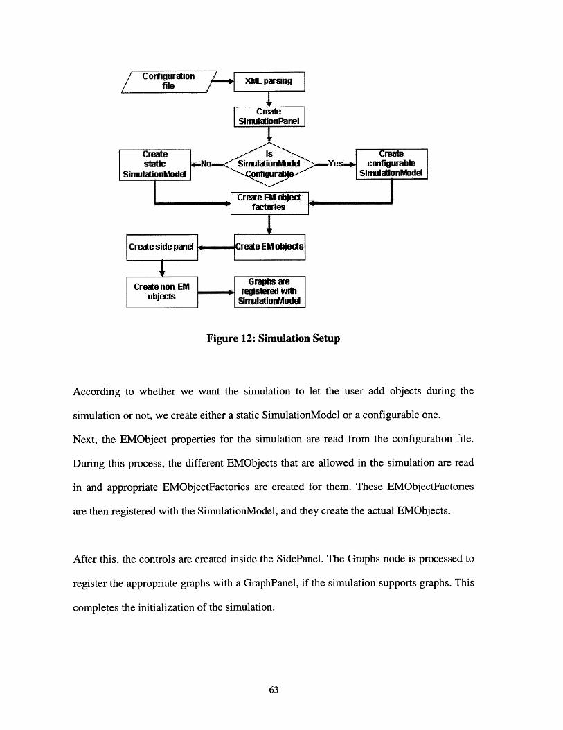
Corfiguatide aiM obrs
CreateSinuiationPane
Create 1 s Creaes a o t c eithe staticSiu lioon n eel Yes configurable
SirNtt E ionb odel ornfiguratl Siar a rm ioniMdel
CreDe EM objectactoriesactories
Creare s de panel S lore lye EM objects.
Afterhe ons aGraphs areC ect EeiteeMwt
SirrulationModel
Figure 12: Simulation Setup
According to whether we want the simulation to let the user add objects during the
simulation or not, we create either a static SimulationModel or a configurable one.
Next, the EMObject properties for the simulation are read from the configuration file.
During this process, the different EMObjects that are allowed in the simulation are read
in and appropriate EMObjectFactories are created for them. These EMObjectFactories
are then registered with the SimulationModel, and they create the actual EMObjects.
After this, the controls are created inside the SidePanel. The Graphs node is processed to
register the appropriate graphs with a GraphPanel, if the simulation supports graphs. This
completes the initialization of the simulation.
63
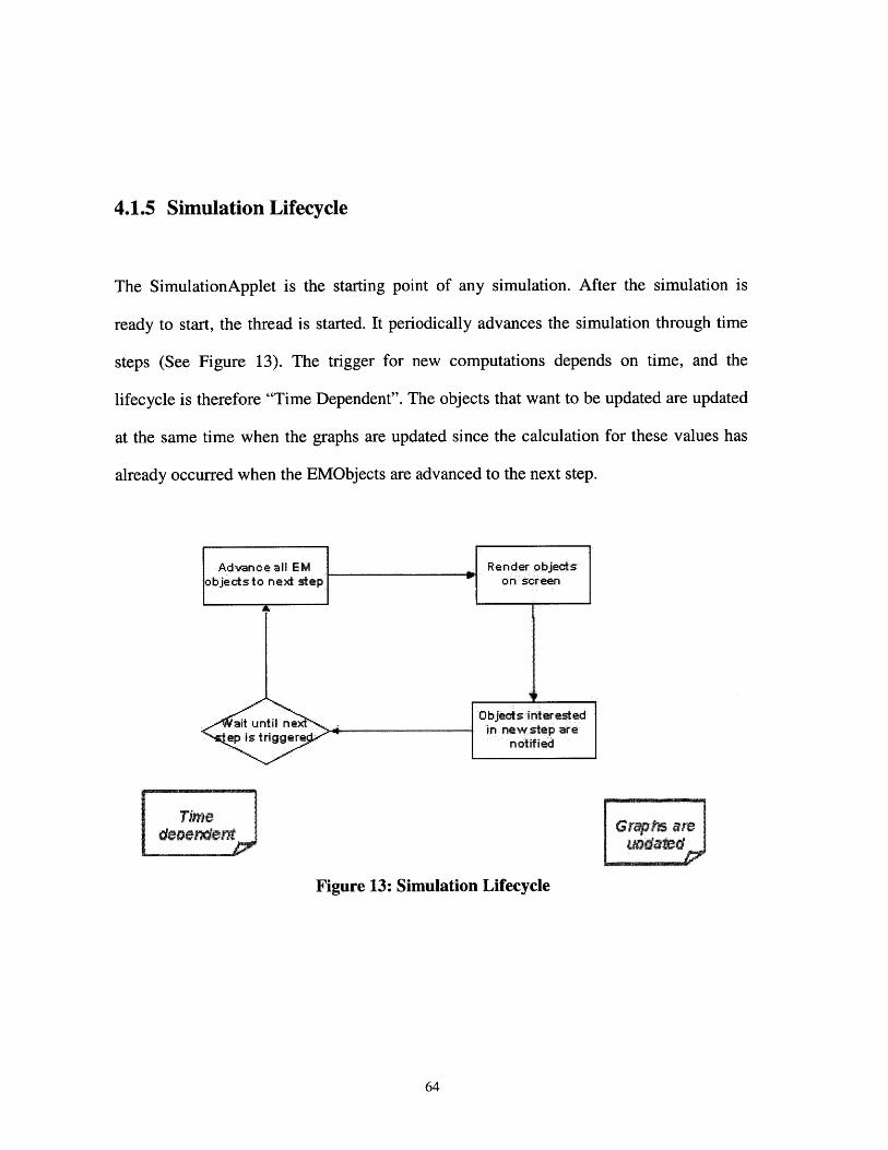
4.1.5 Simulation Lifecycle
The SimulationApplet is the starting point of any simulation. After the simulation is
ready to start, the thread is started. It periodically advances the simulation through time
steps (See Figure 13). The trigger for new computations depends on time, and the
lifecycle is therefore "Time Dependent". The objects that want to be updated are updated
at the same time when the graphs are updated since the calculation for these values has
already occurred when the EMObjects are advanced to the next step.
Advanoe all E M Render objectsobjectsto next step onsreen
ait unti ne0.bjects inerestedep s triderin new sep are
T p istimeenti e
deoeGrphse
Figure 13: Simulation Lifecycle
64
The simulation can be controlled by the different controls added to the SidePanel. As the
simulation progresses, all the different listeners for events or updates are notified when
appropriate events occur. The simulation now proceeds until the user stops it or until a
certain number of simulation steps have been completed.
4.2 Framework Value
4.2.1 Benefits
The software framework brought significant contribution to the developers and non-
developers. The modularity of the software, and the consistent and extensible API used
now make it easy for developers to add or modify the existing functionality without
having to understand the existing code already implemented.
Furthermore, in order to create a new simulation based on the current framework, one
only needs to write an XML file which is human readable, easy to write, and
straightforward. The snippet of code below shows for example how it is possible to create
a new PointCharge in just a few lines of XML code.
<emobject type ="PointCharge"><handler>teal . simulation. emworld. PointCharge</handler><fieldlines draw="true"><symmetry x="false" y="false"/><step size="5"/><point radius="10" angle="1.57"/></ fieldlines></emobj ect>
65
This makes it feasible even for physics teachers to write a new simulation in minimal
time without having to learn Java or understand how the software works. By looking at
an example XML configuration file makes it straightforward to write a new simulation
and start it right away.
4.2.2 Limitations
A few limitations to this software framework were mentioned briefly while explaining
the simulations setup. Here we explain the two main limitations.
4.2.2.1 EMObject Addition Difficulty
When adding a new electromagnetic object to the simulation, this may create undesired
complexities to the computations of the electric and magnetic fields and to the dynamics
of the objects. We have therefore limited the functionality of adding new EMObjects
instead of dealing with trying to solve very complex mathematical equations.
4.2.2.2 Textures Computation Complexity
66
We have seen in section 3.2.3 that different textures were used to illustrate the field lines.
The main limitation is when we want to compute the field line at every point surrounding
the simulation. The number of computations quickly becomes time consuming. We
therefore freeze the simulation when we want to draw such field lines. The computations
took on average around five seconds, and were therefore hindering a smooth continuation
of the simulation.
Nevertheless, when computing only a few field lines such as in Figure 8, the simulation
went on very smoothly since the number of computations was smaller, even though this
simulation is in three-dimensional space. Therefore, we have a tradeoff between the
speed of the computations and the level of detail desired. If zeros are not of interest to us,
we can limit ourselves to a few field lines and have a real-time simulation.
67
Chapter 5
Future Work
The research work for this Master's thesis has a few directions that one can explore to
enhance the existing framework. Some directions would be to:
- Refine the user interface: Asking the students where they feel uncomfortable
and observing whether they are successful at finding the controls they need would
enhance the graphical user interface.
- Add drag-and-drop functionality: The electromagnetic objects are not added to
a simulation as drag-and-drop components. Instead of specifying manually in the
XML file where we want the object to exist, an extension of the work would be to
simplify the coupled mathematical equations in order for the drag- and-drop
functionality to be efficient. As was discussed in section 4.1.3 and 4.2.2.1, adding
a new object makes solving the equations that describe a simulation more
complex.
68
- Simplify algorithms for field lines: The current algorithm for computing field
lines calculates the direction of the field line at a point, travels a certain distance
in that direction, and does the same at the new point. The points are then
connected by line segments. This constrains us to having a considerable number
of points in order to draw smooth field lines. Joining the points by splines would
relieve us from that constraint. We can then have fewer points and fewer
computations, making the simulations run faster.
The initial goal of the simulations was to make the student more active, complement the
laboratory experiments, and help the students understand the concepts that the teacher is
trying to convey in the classroom. We therefore want to make sure that the students
understand the concepts related to the simulations that are presented to them in order to
make sure that they are grasping the intent of the simulation.
The simulations require different levels of proficiency of the student. Instead of
presenting the same simulations to all the students uniformly, we could make sure that
the most appropriate simulation is suggested first, with the freedom for the student to
explore other simulations at different levels of proficiency. We can do this by building a
model of each student, with the model focused on categorizing the student's proficiency.
The entity that can help us build such a model is called a 'tutoring agent'.
In this chapter, we present an area that is worth exploring in order to personalize the
information presented to the students, rather than to consider that at a given time of the
69
academic semester, all the students have a good grasp of all the previous concepts
presented. The appropriate simulations can then be presented to the students for them to
run.
5.1 Student Modeling Goals
In order to understand the level of proficiency of the student, we can build a student
model. The goals of building a model fall under two main areas: delivering the
appropriate information and adapting to the student.
5.1.1 Delivering the Appropriate Information
The learners, as mentioned above, do not all have the same grasp of the material provided
in earlier sessions and simulations. They also fluctuate in their work intensity during the
semester. Therefore, we cannot assume that any previous concepts explained were well
understood by every student.
The simulations that we invite the students to run have different conceptual levels of
difficulty that they are conveying. If the basics are not understood, more elaborate topics
will not be. A useful student model would make inferences about the student's level of
proficiency, and therefore suggest the appropriate simulation to run.
70
5.1.2 Adapting to the Student
Students show patterns of improvements throughout the semester. We can notice for
example continuous improvement, a sporadic one, or other patterns. Trying to incorporate
this information in the student model would help anticipate the coming improvements,
and therefore allow us to present more or less complicated topics to the student.
In addition, students have different backgrounds depending on the classes they have
taken previously and their personal knowledge. Having some background knowledge of
the students would help us build a better model of them and start from that model rather
than from scratch.
5.2 Tutoring Agents
After decades of work, programmers were able to build a computer system that beat the
world chess champion. The question is whether it is possible to create an intelligent
tutoring system that is better than the teacher in a given subject. Paul Goodman, director
of the Institute for Strategic Development at Carnegie Mellon University, argues that this
is indeed possible [15]. Tutoring agents are a special class of software agents aimed at
teaching.
In order to understand software agents, let us understand their features [16]:
71

- One must be able to communicate with the agent. Both the human subject and the
agent must speak the same language. Any agent that cannot understand what one
wants to accomplish will be of little help.
- The agent must be able to act and suggest. Taking the analogy with a travel agent,
a customer expects the agent to be able to book flights, hotels and rent cars. A
travel advisor in contrast only advises which are the best flights, hotels and car
rentals.
- An agent can do things without supervision. If a customer wants to book a
complex trip through a travel agent, which requires one to be on the phone while
all details were planned and finalized, it would take a considerable amount of
time. Instead, the agent should be able to do its work without consuming the
customer's time.
- A key ability of good agents is their experience. If a customer travels a lot, the
travel agent should learn about this person's preferences. But further, the best
agents learn how much, or how little, the customer wants them to do.
Although the tasks that software agents carry out seem fairly easy to visualize, the
construction of the agents themselves is somewhat more problematic. Agent programs
differ from most software mainly by what we can best describe as a sense of themselves
as independent entities [23]. An agent should also be robust and adaptive [12], capable of
72
learning from experience and responding to unforeseen situations with a repertoire of
different methods. Finally, it should be autonomous so that it can sense the environment
and act independently of it in order to be able to make progress towards its goal.
In an educational environment, a tutoring agent should observe the habits of the student,
understanding her proficiency level, and suggest the information that would benefit the
student most. If the agent notices a lack of understanding of fundamental concepts, it
would suggest to the student to learn about them first before exploring more advanced
topics.
The agent's activity can range from very active to passive, a simple observer [1]. This
depends on how comfortable the student feels when dealing with the agent [20]. Some
people like to work at their own pace, and explore resources without any help. An
example would be the Microsoft Office "paper clip" agent that people either like or
dislike.
5.3 Tutoring Agent Design
The difference in the levels of proficiency of students makes each of them a unique
person to be targeted with specific information. The proposed design consists of an agent
object that interacts with one student, learns from this student, and is therefore capable of
building a model of that student.
73
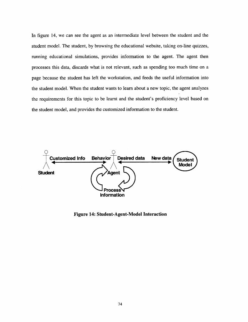
In figure 14, we can see the agent as an intermediate level between the student and the
student model. The student, by browsing the educational website, taking on-line quizzes,
running educational simulations, provides information to the agent. The agent then
processes this data, discards what is not relevant, such as spending too much time on a
page because the student has left the workstation, and feeds the useful information into
the student model. When the student wants to learn about a new topic, the agent analyzes
the requirements for this topic to be learnt and the student's proficiency level based on
the student model, and provides the customized information to the student.
Customized Info Behavior Desired data New data Student-1% 1 \i odel
Student Agent
ProcessInformation
Figure 14: Student-Agent-Model Interaction
74
5.3.1 Design Areas
The agent keeps a record of the student every time the software is accessed. Previous
information is not deleted. This allows the agent to follow the progress of the student
[17]. If we are designing a website from which the simulations are delivered, a
connection between the agent and a database about the student is crucial. A channel
provides communication between the client, the agent, the server, and the database.
The system gives advice on which simulations to run first, or it can add some extra
explanation of terms for which the student has not yet read the definition [10].
The agent has also the option to be shut down [13] . In that case, it ceases making
suggestions; instead, it records the progress and the habits of the student 'silently'. These
are stored, and used later on if the student changes her mind and wants the tutoring agent
to interact with her again. The agent will in that case be prepared, have background
information about the student, and be efficient at suggesting the appropriate simulations.
In addition, the student's level of proficiency is assessed by short quizzes and by
recording the progress of the student. In the case of a website equipped with a search
engine, the agent monitors words that are typed more frequently than others, and maps
them into the existing database of technical words. If many occurrences of one topic
75
occur, the agent identifies it, searches the database for related material, and presents this
material to the student.
A good design to work on is collaboration between tutoring agents [19]. Since each
tutoring agent is assigned to a student, they can share information on whether a particular
set of simulations presented was more successful than others in the student's
understanding of the concepts. This understanding can be measured by the answers to the
conceptual questions in quizzes, short tests and dynamic questions that pop up during the
simulation. This last measurement will be further explored in section 5.5.
5.3.2 Advantages Over Previous Work
Previous work has focused on a few areas discussed in section 5.3.1, therefore having
some aspects of a fully functional agent. The advantage of our proposed approach is that
we join all the proposed aspects of building a comprehensive student model, following
the student's progress, making the agent privacy-enabled, and creating collaboration
among different agents. Bringing all these aspects together provides a way for the student
to get the information most relevant in a fast fashion. The collaboration of the tutoring
agents makes the agents learn faster about 'their' students, and therefore able to deliver
the proper information after a shorter period.
5.4 Student Model Design
76
The parameters of interest that help build the student model focus on the student's
proficiency. We can measure that proficiency by observing the registration details, the
quizzes results, and the student's progress.
5.4.1 Registration details
Before starting to have the agent build the student model, the learner is asked a series of
questions that helps categorize the student to fit a certain proficiency level [25]. The
questions focus on the background of the student, her familiarity with the material taught
in class and her knowledge about a few basic concepts the class requires. For example,
questions are asked about the student's mathematical background required in order to feel
comfortable with some mathematical manipulations.
This questionnaire can be as trivial as a few questions that give us an idea about certain
topics, or as advanced as a knowledge-based system where questions are dynamically
generated, and help build a model of the student's proficiency with a certain level of
confidence after each answer by the student. This questionnaire can be used as a starting
point of the student's model building.
5.4.2 Quizzes
77
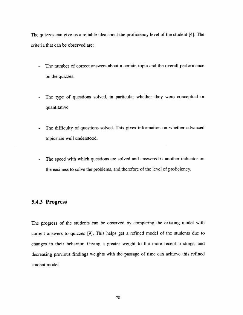
The quizzes can give us a reliable idea about the proficiency level of the student [4]. The
criteria that can be observed are:
- The number of correct answers about a certain topic and the overall performance
on the quizzes.
- The type of questions solved, in particular whether they were conceptual or
quantitative.
- The difficulty of questions solved. This gives information on whether advanced
topics are well understood.
- The speed with which questions are solved and answered is another indicator on
the easiness to solve the problems, and therefore of the level of proficiency.
5.4.3 Progress
The progress of the students can be observed by comparing the existing model with
current answers to quizzes [9]. This helps get a refined model of the students due to
changes in their behavior. Giving a greater weight to the more recent findings, and
decreasing previous findings weights with the passage of time can achieve this refined
student model.
78
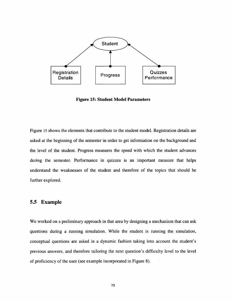
Student
Registration Progress Q uizzesDetails Performance
Figure 15: Student Model Parameters
Figure 15 shows the elements that contribute to the student model. Registration details are
asked at the beginning of the semester in order to get information on the background and
the level of the student. Progress measures the speed with which the student advances
during the semester. Performance in quizzes is an important measure that helps
understand the weaknesses of the student and therefore of the topics that should be
further explored.
5.5 Example
We worked on a preliminary approach in that area by designing a mechanism that can ask
questions during a running simulation. While the student is running the simulation,
conceptual questions are asked in a dynamic fashion taking into account the student's
previous answers, and therefore tailoring the next question's difficulty level to the level
of proficiency of the user (see example incorporated in Figure 8).
79
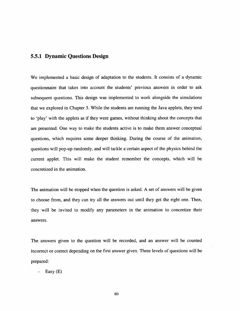
5.5.1 Dynamic Questions Design
We implemented a basic design of adaptation to the students. It consists of a dynamic
questionnaire that takes into account the students' previous answers in order to ask
subsequent questions. This design was implemented to work alongside the simulations
that we explored in Chapter 3. While the students are running the Java applets, they tend
to 'play' with the applets as if they were games, without thinking about the concepts that
are presented. One way to make the students active is to make them answer conceptual
questions, which requires some deeper thinking. During the course of the animation,
questions will pop-up randomly, and will tackle a certain aspect of the physics behind the
current applet. This will make the student remember the concepts, which will be
concretized in the animation.
The animation will be stopped when the question is asked. A set of answers will be given
to choose from, and they can try all the answers out until they get the right one. Then,
they will be invited to modify any parameters in the animation to concretize their
answers.
The answers given to the question will be recorded, and an answer will be counted
incorrect or correct depending on the first answer given. Three levels of questions will be
prepared:
- Easy (E)
80
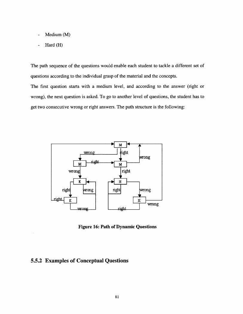
- Medium (M)
- Hard (H)
The path sequence of the questions would enable each student to tackle a different set of
questions according to the individual grasp of the material and the concepts.
The first question starts with a medium level, and according to the answer (right or
wrong), the next question is asked. To go to another level of questions, the student has to
get two consecutive wrong or right answers. The path structure is the following:
ong
wrong right
E H
righl t!]g ng
E Hwng
Figure 16: Path of Dynamic Questions
5.5.2 Examples of Conceptual Questions
81

We mentioned conceptual questions in different parts of the thesis. These are some
examples of how the conceptual questions would look like. Note that they are qualitative
in nature and drive the student to think about the material explained in class.
Question 1: The magnetic field lines shown are distorted when the electric charge is near
them. This happens because:
1. The field lines of the magnet get caught on the charge when it moves past them.
2. The magnetic field lines shown represent the total field and the magnetic field of
the charge is largest close to the charge.
3. The magnetic field lines of the magnet are attracted to the electric charge because
of Coulomb's Law.
Question 2: If you double the speed of the charge in the x-direction or y-direction, what
will happen to the radius of the small circle around which the charge rapidly moves?
1. It will increase
2. It will decrease
3. It will stay the same.
Question 3: The charge moves in small circles around the field, but it also moves slowly
around in the equatorial plane of the magnet. Why does this happen?
82
1. When the charge moves closer to (further from) the magnet the field strength goes
up (down) and the small circular orbit becomes smaller (larger) in radius. The
combination of these two effects causes a drift in longitude about the magnet.
2. When the charge moves closer to (further from) the magnet the field strength goes
up (down) and the small circular orbit becomes larger (smaller) in radius. The
combination of these two effects causes a drift in longitude about the magnet.
3. When the charge moves closer to (further from) the magnet the speed of the
charge goes up (down). The combination of these two effects causes a drift in
longitude about the magnet.
5.6 Conclusion
This thesis presented a framework for electromagnetism simulations, the benefits these
simulations bring to conceptual understanding and their practicality and appeal for the
students. We hope the simulations were beneficial to the students, and that they will be
able to still remember electromagnetism concepts in a few years.
We also presented a direction of future research in which a tutoring agent presents the
appropriate simulations according to the student's proficiency level, instead of following
the curriculum of the class without consideration of the student's understanding of
previous basic concepts.
83

84
References
[1] Andr6, E., Rist, T., and MUller, J., Integrating reactive and scripted behaviors inlife-like presentation agents. In K.P. Sycara and M. Wooldridge (Eds.),Proceedings of the Second Int'l Conf on Autonomous Agents, pp. 261-268, 1998.
[2] Athabasca University: Internet undergraduate courses. URL athttp://www.athabascau.ca/main/procrs.htm.
[3] Beaty, W.J., "Popular Culture, K-6 Textbooks and "Science myths"", 1996.
[4] Beck, J. and Woolf, B., "Using a Learning Agent with a Student Model",Intelligent Tutoring Systems, 6-15, 1998.
[5] Belcher, J., "Project Proposal of TEAL", URL: http://caes.mit.edu/research/teal/.
[6] Belcher, J., "Studio Physics at MIT", Physics News Letter Article, 2001.
[7] Belcher, J., Olbert, S. and Bessette, M., "The Physics Of Using Field LineAnimation In The Teaching Off Electromagnetism", American Association OfPhysics Teachers Meeting January, 1999.
[8] Bigelow, J.D., "Developing in Internet section of a management course:Transporting learning premises across media", World Conference of the WebSociety Proceedings, AACE, pp. 13-20, 1996.
[9] Brusilovsky, P., "Methods and Techniques of Adaptive Hypermedia", UserModeling and User-Adapted Interaction 6, 87-129, 1996.
[10] De Bra, P.M.E., "Teaching hypertext and hypermedia through the Web", WorldConference of the Web Society Proceedings, AACE, 130-135, 1996.
[11] Dori, Y. and Belcher, J., "Assessing the Effect of TEAL Project on Students'Understanding of Physics Concepts",http://web.mit.edu/jbelcher/www/iCampus/TEALAssessmentFeb2002.pdf, not yetpublished.
[12] Eliot, C., and Woolf, B.P., "An adaptive student centered curriculum for anintelligent training system", User Modeling and User-Adapted Interaction, 5:67-86, 1995.
85
[13] Foner, L., "Clustering and Information Sharing in an Ecology of CooperatingAgents", Proceedings of 1995 Conference on Computers, Freedom, and Privacy,March 1995.
[14] Frost, R. and Cutkosky, M. R., "Design for Manufacturability via AgentInteraction," paper no. 96-DETC/DFM-1302, Proc. 1996 ASME Computers inEngineering Conf, ASME, New York, pp. 1-8, 1996.
[15] Goodman, P., "Technology Enhanced Learning: Opportunities for Change",August 2001.
[16] Hendler, J., "Is There an Intelligent Agent in Your Future?" Nature @ Macmillan,March 1999.
[17] Johnson, W L & Shaw, E., "Using Agents to Overcome Deficiencies in Web-Based Courseware", IJCAI-97 Animated Interface Agents Workshop 1997.
[18] Johnson, W. L., Rickel, J., Stiles, R., and Munro A., "Integrating pedagogicalagents into virtual environments", Presence 7(5), 1998.
[19] Lashkari, Y., Metral, M., Maes, P., "Collaborative Interface Agents", AAAI 1994,444-449, 1994.
[20] Lester, J.C., Converse, S.A., Kahler, S.E., Barlow, S.T., Stone, B.A., and Bhogal,R.S., "The persona effect: Affective impact of animated pedagogical agents",Proceedings of CHI '97, pp. 359-366. ACM Press, 1997.
[21] Lieberman, H., Van Dyke, N.H. and Vivacqua A., "Let's Browse: A CollaborativeWeb Browsing Agent," IUI'99, 1999.
[22] Linturi, R., "Network Society has new tools for learning, but it also redefineswhat learning means", Enabling network-based learning, Enable99, 1999.
[23] Maes, P., "Intelligent Software: Programs That Can Act Independently Will Easethe Burdens that Computers Put on People". Scientific American 273 (3): 84-86,1995.
[24] McDermott, L., "Research in Physics Education", The American Physical Society,1998.
[25] Mitrovic, A., "INSTRUCT: Modeling Students by Asking Questions", UserModeling and User-Adapted Interaction, Vol. 6, No. 4, pp. 273-302, 1996.
[26] Nakhleh, M.B. and Mitchell, R.C., "Concept learning versus problem solving",Journal of Chemical Education, 70(3), 190-192, 1993.
[27] Niemzcick, S., "Using Markov Models to Classify Usage Patterns inCourseware", not yet published.
86
[28] Nurrenbern, S. C. and Pickering, M., "Concept learning versus problem solving:Is there a difference?" Journal of Chemical Education, 64(6), 508 - 510, 1987.
[29] Pickering, M., "Further studies on concept learning versus problem solving: Isthere a difference?" Journal of Chemical Education, 67, 254-255, 1990.
[30] Rakel: Rakel's online textbook of medicine:http://www.usc.edu/hsc/medicine/family med/textbook
[31] Rhodes, B. and Maes, P., "Just-in-time information retrieval agents", IBMSystems Journal special issue on the MIT Media Laboratory, Vol. 39, Nos. 3 and4, pp. 685-704, 2000.
[32] Ritter, S., du Boulay, B.. and Mizoguchi, R.., "Communication, cooperation, andcompetition among multiple tutor agents", Artificial Intelligence in Education,31-38, 1997.
[33] Shaw, E., Johnson, W. E., and Ganeshan, R., "Pedagogical Agents on the Web".Proceedings of the AI-ED Workshop on Pedagogical Agents, pp. 48-55, Kobe,Japan, 1997.
[34] Yehudit Dori, John Belcher, "Assessing the Technology Enabled Active LearningProject", not yet published.
87