TECHNOLOGY DEVELOPMENT FOR

EXOPLANET MISSONS

Technology Milestone Report

Visible Nuller Coronagraph Technology Demonstration

Jagmit Sandhu, P.I. Michael Shao

1 May 2015

National Aeronautics and Space Administration

Jet Propulsion Laboratory

California Institute of Technology

Pasadena, California

© Copyright 2015 California Institute of Technology. Government sponsorship

acknowledged.

1

Table of Contents

1. Executive Summary 2

2. Objective 3

3. Introduction 3 3.1. Technical Approach and Methodology 3

3.1.1 Visible Nulling Coronagraph Architecture 4 3.1.2 Speckle Suppression 8

4. Milestone Report 11 4.1. APEP Testbed 11

4.1.1 Deformable Mirror 13 4.1.2 Lyot Stop 14 4.1.3 Fiber Array 15

4.2. Experiment Description 21 4.2.1 DM phase response 21 4.2.2 PZT phase response 22 4.2.3 Nuller Intensity matching 23 4.2.4 Null Acquisition 31 4.2.5 Post-Coronagraph Calibrator 34 4.2.6 Discussion 34

4.3. Future Work 36 4.4. Specifications of some Key Components 38

5. References 39

6. Acronyms 41

2

TDEM Milestone Report:

Visible Nulling Coronagraph Technology

1. Executive Summary

This report summarizes the results of experiments undertaken on the APEP testbed at JPL to further development of high contrast coronagraphy using interferometric nulling and an array of spatial filters. This technology is especially suitable for implementing a coronagraph on centrally obscured and/or segmented telescopes. The advantage arises by use of a segmented deformable mirror (DM) and an array of spatial filters comprised of individual single mode fibers. This allows division of the telescope pupil into sub-apertures that can be nulled independently while a Lyot Stop is used to reject parts of the pupil that are obscured. Thus segment gaps, spiders and central obscurations can be easily ignored for the purpose of nulling. The combination of the DM and spatial filters also leads to the formation of a 360 degree dark hole without the need of a second DM.

While nulling has been demonstrated in prior experiments, the use of a 2-D array of single mode fibers in combination with the nuller is unique and challenging. Early in our experiments we discovered that the fiber array installed in APEP was deficient in its role as a spatial filter. The lengths of the fibers were too short to enable sufficient filtering of cladding light in the filters. Single fiber experiments were then conducted to measure the length of fiber necessary for extinction of cladding light to 10

-4. The results indicated that

fibers with length between 1 to 2 m would be needed. We therefore had to explore novel methods to fabricate a new fiber array with sufficiently long fibers while simultaneously ensuring that all the fibers were equal to within the criteria needed to produce a coherent wavefront for planet light (the nulling of starlight does not care about the coherence since nulling occurs independently in each fiber).

We adopted a dual-pronged approach of building a quick, incoherent fiber array to demonstrate and uncover issues with starlight nulling, while also building a coherent fiber array to be used for the final demonstration. Both arrays also presented the challenge of fabrication of microlenses. Each microlens had to be positioned to +/- 0.5 um of the center of the corresponding fiber. Additionally, each fiber is potentially offset randomly from the ideal grid by +/- 10 um. We developed a measurement system that measured the fiber positions with the accuracy necessary for this purpose. We then had to develop a new microlens fabrication technique (thermal reflow of photoresist) because the traditional technique (etching of fused silica) could not meet the microlens sag requirement. We fabricated, aligned and bonded microlenses to the incoherent array and conducted nulling experiments. We were able to demonstrate mean contrast between 2x10

-7 and 6x10

-7. This was mainly limited by instability of the intensity distribution of

starlight in the pupil and possible polarization mis-match between the interfering beams. Lack of time and resources did not allow us to fabricate microlenses and conduct similar experiments with the coherent array, as well as the post-coronagraph calibrator interferometer that we had proposed for this TDEM.

3

2. Objective

In support of NASA’s Exoplanet Exploration Program (ExEP) and the ROSES Technology Development for Exoplanet Missions (TDEM), this document reports the technical work undertaken for the Visible Nulling Coronagraph (VNC) Technology Demonstration project.

3. Introduction

TDEM Technology Milestones are intended to demonstrate significant advances in the current state of the art of extra-solar planet imaging techniques. Coronagraphs are among the key promising technologies for the detection of exoplanets. The VNC is one of the coronagraph architectures that have been extensively studied for exoplanet detection, both for ground based astronomy and space based missions. The VNC, and its close ancestor, Nulling Interferometry, have also been in development in laboratories for many years in different manifestations and wavelength ranges. Our proposal aims to demonstrate the potential of a VNC to suppress starlight to a contrast of 3x10

-8. This will

be accomplished through a series of experiments using a VNC in an existing ExEP facility at JPL – the APEP testbed. We will demonstrate a progression of increasing contrast levels using laser and white light with the existing testbed. Concurrently we will design and build a wavefront sensor to achieve higher SNR wavefront control and enable post-detection speckle subtraction that will ultimately demonstrate the target contrast of 3x10

-9. Completion of this milestone is to be documented in a report by the Principal

Investigator and reviewed by the Exoplanet Exploration Program.

Note: The name APEP is derived from the ancient Egyptian diety Apep – the deification of darkness and chaos, and thus the opponent of light and truth. We use the darkness/light interpretation.

This milestone reads as follows:

Milestone 1 definition: Narrowband Starlight Suppression with VNC

Demonstrate a raw coronagraph contrast of 310-8

(with a goal of 310-9

) with the

VNC at angular separations of 2D tD, using 2% bandwidth light (somewhere

in the wavelength range 650 – 800 nm), for one polarization state.

The angular separations are defined in terms of the central wavelength of the passband 650 – 800 nm, i.e. 725 nm, and the diameter D of the aperture stop as defined by the diameter of the single mode fiber array in the VNC. This demonstration will preferably be done with a pupil shear of 25% (of D) but only if a white light source can be procured that offers sufficient brightness when expanded and sheared that the sheared pupils do not differ in intensity at any point in the pupil by more than 0.5%. Otherwise the demonstration will be done with no shear.

3.1. Technical Approach and Methodology

In the following sections we describe how a VNC rejects starlight, followed by an explanation of our proposed wavefront sensor. We also describe the status of the APEP testbed and the experimental progress made under the current TDEM. Most of these sections

4

are borrowed from the white paper document written for this TDEM. We include them here for easy reference on the basics of the VNC architecture.

3.1.1 Visible Nulling Coronagraph Architecture

A Visible Nulling Coronagraph is essentially a nulling interferometer operating at

visible wavelengths. The interferometer provides the ability to reject starlight. In its

simplest design, the VNC can be operated with a single deformable mirror. This yields

the well known single-sided dark hole in the image plane. In a further refinement, the

VNC can be followed by an array of spatial filters. This simplifies the starlight rejection

algorithm, while yielding a 360-degree dark hole. This has obvious advantages with

respect to the time spent in any space coronagraph mission in searching for exoplanets.

We have chosen to pursue the latter approach. The spatial filter array in our case is an

array of single mode fibers with input and output coupling microlenses. The spatial filters

divide the telescope pupil into multiple sub-apertures that can be nulled independently.

This leads to a very simple rejection of telescope pupil obscurations via use of a matching

Lyot Stop on the input side of the spatial filter array.

Nulling Interferometer

A nulling interferometer destructively interferes the light from two collecting apertures. Figure 1 illustrates the case of a two-telescope nuller. Introduction of a π phase shift in one arm of the interferometer (using an extra path length delay) leads to destructive interference of on-axis light. Light from an off-axis source, such as a planet, does not achieve that same phase shift concurrent with the on-axis source. A subsequent imaging detector will show very little evidence of the central star but will reveal any close-by companions. A simple 2-element nuller has a sinusoidal transmission pattern on the sky:

BkkT

2),cos(1)(

= angular separation of the

companion from star. Baseline B is

the separation between the two

apertures. A correct baseline length

can put the planet on the first bright

fringe. This fringe location

corresponds to B = /(2 ). For an

Earth-Sun system at 10 parsec, =

0.1 arcsec, and if observing at =

600 nm, we would need B = 62 cm.

Therefore the configuration in

figure 1 is not practical for planet

detection because the separation between telescopes are rather small ~ 60 cm, while the

needed collecting apertures (for adequate SNR on the planet) are quite large ~ 4 m. An

Figure 1 Schematic outline of a Nulling

Interferometer, with the associated fringe

transmission pattern on the sky shown below. In

practice the star would be placed at the null of the

fringe and the planet at the maximum.

5

additional problem with this setup is the need to rotate the baseline around the line of

sight in order to image planets at all possible azimuthal angles.

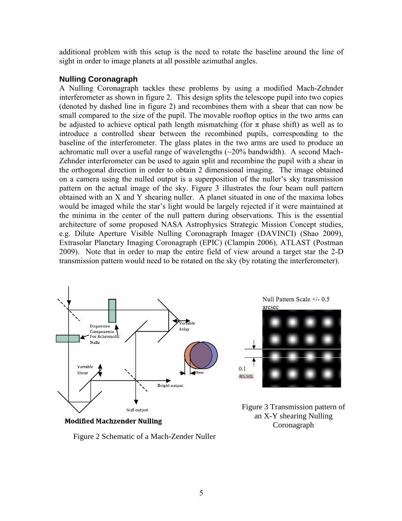
Nulling Coronagraph A Nulling Coronagraph tackles these problems by using a modified Mach-Zehnder

interferometer as shown in figure 2. This design splits the telescope pupil into two copies

(denoted by dashed line in figure 2) and recombines them with a shear that can now be

small compared to the size of the pupil. The movable rooftop optics in the two arms can

be adjusted to achieve optical path length mismatching (for π phase shift) as well as to

introduce a controlled shear between the recombined pupils, corresponding to the

baseline of the interferometer. The glass plates in the two arms are used to produce an

achromatic null over a useful range of wavelengths (~20% bandwidth). A second Mach-

Zehnder interferometer can be used to again split and recombine the pupil with a shear in

the orthogonal direction in order to obtain 2 dimensional imaging. The image obtained

on a camera using the nulled output is a superposition of the nuller’s sky transmission

pattern on the actual image of the sky. Figure 3 illustrates the four beam null pattern

obtained with an X and Y shearing nuller. A planet situated in one of the maxima lobes

would be imaged while the star’s light would be largely rejected if it were maintained at

the minima in the center of the null pattern during observations. This is the essential

architecture of some proposed NASA Astrophysics Strategic Mission Concept studies,

e.g. Dilute Aperture Visible Nulling Coronagraph Imager (DAVINCI) (Shao 2009),

Extrasolar Planetary Imaging Coronagraph (EPIC) (Clampin 2006), ATLAST (Postman

2009). Note that in order to map the entire field of view around a target star the 2-D

transmission pattern would need to be rotated on the sky (by rotating the interferometer).

Figure 3 Transmission pattern of

an X-Y shearing Nulling

Coronagraph

Figure 2 Schematic of a Mach-Zender Nuller

6

Control of scattered light

The null depth of a nulling coronagraph is defined as the ratio of minimum to

maximum intensity of the nulled output (i.e. maximum destructive to maximum

constructive interference). The null depth is a function of the phase and intensity

mismatch between the two arms (Serabyn 2000):

is the phase mismatch between the two arms, and is the relative intensity mismatch of the two arms (intensity difference divided by mean intensity). Figure 4 illustrates this 2-dimensional dependence of N. For example, N = 10

-7 can be achieved

with = 50 pm and = 7x10-4

.

It is important to point out that the null depth is not the same as the contrast ratio that is of importance in planet detection and as it is written in the milestone. Contrast is a comparison of the stellar PSF peak intensity to the intensity some distance away, at a position that would be relevant for observing the planet. This separation is usually stated in units of resolution elements of the telescope, /D. Since the Airy disk PSF decreases away from the center, this position offset provides another level of rejection of starlight. The closer to the center of the PSF, the lower the rejection. Hence the challenge with building a coronagraph to work at small /D. At very high contrast levels the stellar Airy disk is replaced by speckles caused by imperfect nulling and these ultimately set the contrast floor. In our proposal we are aiming for high contrast performance at 2 /D (which corresponds to a pupil shear of 25%). This separation provides a rejection factor

Equation 1 Null Depth of Nulling Coronagraph

Figure 4 Null Depth as function of OPD and Relative Intensity

Difference (log scale)

7

of at least 5x10-3

for an Airy disk. The corresponding contrast using a null depth of N = 10

-7 is 5x10

-10.

Clearly equation 1 implies that high levels of starlight suppression require very accurate optical surfaces in both phase and amplitude. The assumption that such precise optical surfaces are available, especially for 4 m or larger sized telescopes, is not true. However there is a way to circumvent these problems. If the output of a nulling interferometer is focused onto a single mode fiber, then inside the fiber the only parameters that are important are the amplitude and phase of the electric field. If the amplitude and phase are properly matched a very deep null can be achieved. The problem has been reduced to just two degrees of freedom. But a single fiber will not provide imaging capability. To actually image an exoplanet a coherent array of single mode fibers is needed. Such an array is illustrated in figure 5.

The pupil of the telescope would be re-imaged onto a microlens array that focuses the light onto corresponding single mode fibers. Each single mode fiber cleans up the wavefront entering the corresponding microlens. To achieve the phase and amplitude match required for deep nulls we need to control the tip, tilt and phase of the wavefront impinging on the input microlens for each fiber. This is done by replacing a continuous reflective surface in one arm of the nuller with a segmented mirror. Figure 6 shows the schematic of a nuller using a segmented deformable mirror (DM). One segment of the DM maps exactly to one microlens and fiber. With this arrangement wavefront errors at high spatial frequency, on a spatial scale smaller than a DM segment, will be filtered by the single mode fibers instead of propagating through to the science focal plane. If the optical fibers all have the same length (within /4) the planet light from each fiber combines to form a coherent off-axis image. The phase of the residual starlight exiting the fiber array is random, hence it is scattered evenly across the whole field of view. Chopping between the two arms of the nuller gives us the intensity ratio of the two light beams for each fiber. The DM segments are then controlled in tip and tilt to vary the amount of light coupling into the fibers until the intensity of the nuller’s DM arm matches that of the reference arm. Subsequently the segments are controlled in piston only to maintain a π phase shift with respect to the reference arm. The pupil camera is the wavefront sensor and looks at an image of the recombined pupil. The one to one correspondence between the DM segments and the fibers along with the independence of

Figure 5 Principal of Spatial Filter Array. Input wavefront and amplitude aberrations are

converted into intensity variations and stepwise phase at the output

8

each segment and fiber combination from all other segments and fibers naturally lends itself to wavefront sensing in the pupil plane as compared to speckle nulling in the image plane of the science camera (as is seen in some Lyot coronagraphs).

Several investigators have implemented different versions of a nulling coronagraph. Most have been limited to single fiber experiments. Our own prior experiments with single fiber nulling have yielded suppression of laser light to 1.25x10

-7 and white light

(15% passband) to 10-6

(Samuele 2007). Recently Lyon (2009) has reported narrow band nulling to 10

-6 with a 163 segment DM but without a fiber array (single-sided dark hole).

3.1.2 Speckle Suppression

The conventional wisdom is that an earth-like exoplanet can be imaged with a coronagraph that suppresses starlight to 10

-10, about the contrast level of an exo-Earth.

This nominal notion of the requirement for a coronagraph is incorrect. If the average scattered light in the coronagraph’s image plane is 10

-10, there will be 100’s of speckles

whose brightness is equal to that of an exo-Earth. Hence speckle suppression has to be achieved to a contrast of 10

-11 for an exo-Earth to be detected with < 1% false alarm

probability. All coronagraphs have two means of speckle suppression – optical and/or post-detection. Optical suppression attempts to prevent speckle formation via ultra-precise control of the wavefront. The fundamental limitations to active wavefront control are photon noise and the thermal stability of optics. The former needs a bright source and the latter is a challenge considering the stability required ~ even a sinusoidal ripple of 1 pm in the pupil can induce speckles of ~10

-10. Typical lab conditions are easily factors of

10-100 worse for optical path length stability. Hence optical suppression alone cannot get us to the target contrast levels of < 10

-10. We must combine optical speckle suppression

with post-detection speckle subtraction. In this technique the speckles due to remnant starlight are measured contemporaneously with the science image. In later data processing these speckles are subtracted from the science image, yielding the final high contrast image.

With this motivation in mind we propose to implement a post-coronagraph wavefront sensor (called the Calibrator) that utilizes both the dark and the bright outputs of the nuller, as show in Figure 7. The Calibrator serves to generate correction signals for the

Figure 6 Schematic of Nulling Coronagraph

with Fiber array and Segmented Mirror

9

nuller control loop as well as measure the remnant stellar speckles for later subtraction from the science image. The essential idea is to interfere the remnant starlight from the dark output of the nuller with a coherent reference wavefront. Additionally, with a bright reference wavefront the phase measurements can be made in a photon noise limited regime. The bright output is spatially filtered through a pinhole (diameter ~10 um) to preserve only the low order wavefront. The light in the bright output is dominated by starlight and since planet, exo-zodi and local zodi light are incoherent with starlight, the wavefront after the spatial filter is only coherent with the starlight in the dark output. A subsequent beam combiner is used to interfere the two beams. The image in the pupil camera is therefore a measurement of the starlight that leaks through the dark output.

One mirror in the reference arm is capable of precision dithering so that we can gather fringe data at two or more phase offsets. This enables calculation of the phase map and intensity, yielding the full electric field. The phase map allows generation of real time correction signals for the DM in the nuller while a Fourier transform of the electric field is equivalent to the residual speckles due to starlight leakage in the science camera (after calibration). The optical train stability requirement has thus been reduced from long term ~ 2 hours per visit, to the time scale of the nuller closed loop ~ 60 seconds, nearly a factor of 100.

Several authors have proposed and implemented this concept in one form or another. (Guyon 2004, Wallace et al. 2006, Vasisht et al. 2006, Rao et al. 2008). The Gemini Planet Imager will have a post-coronagraph wavefront sensor much like the calibrator outlined above (Wallace et al. 2008). A very similar sensor has been built for the P1640 coronagraph on the Palomar 5m telescope (Hinkley et al. 2011, Crepp et al. 2011, Pueyo et al. 2012). The P1640 papers report factor of 10 improvements in speckle suppression via post processing. These sensors were built at JPL and our team has contributed directly to these projects and is intimately familiar with the details of implementation and successful operation. Rao (2008) discuss a method whereby they use visibility data in the calibrator to generate DM correction signals since that metric is immune to exact starting phase in the calibrator. We intend to explore several algorithms that we have used in

Figure 7 Schematic of Nulling Coronagraph with

post-coronagraph wavefront sensor

10

different projects where we have implemented this design. Initial results with the P1640 coronagraph using reconstruction of the PSF on Alpha Cyg have shown reduction of static speckles by a factor of ~5 to 10 (private communication).

11

4. Milestone Report

4.1. APEP Testbed

The VNC experiments for this project were undertaken in the APEP testbed at JPL. Figure 8 shows part of the testbed and figure 9 is the optical layout. Light launched from a single mode fiber is collimated by an off axis parabola (OAP). A linear polarizer ensures that only light with s polarization (i.e. perpendicular to the optical table surface) is launched into the nuller. Each arm of the nuller has a roof top mirror assembly and a carefully designed pair of glass plates of different refractive indices to enable control of dispersion. The plates have wedges such that when they are moved perpendicular to the light beam a varying amount of glass can be used to match dispersion and thereby satisfy the π phase shift condition over the wavelength range of 650 to 800 nm. Until now the experiments have been done in laser light so that this dispersion-matching step has not been needed.

The DM is used to control the shape of the wavefront for intensity and phase matching of the two arms of the nuller. The non-DM arm of the nuller (the reference arm) has a flat mirror on a piston, tip and tilt mount assembly. This mirror is used to match tip/tilt of the wavefront to that of the wavefront in the DM arm and also for achieving π optical path difference (OPD) in the nuller. During operation this mirror is dithered in 4 steps of π/2 phase shifts at the center wavelength to enable phase calculation by the real time control system using the pupil camera images. The phase values are converted to motion commands for the DM actuators and sent to update the DM in time for the next iteration of the 4-step dither cycle. Once the null has been acquired this 4- Figure 8 APEP testbed in its vacuum chamber

12

step dither cycle is suspended so that science camera data can be collected and the null metrics measured.

The dark output of the nuller is imaged onto a Lyot Stop that blocks light corresponding to the DM segment edges, defective DM segments and defective fibers/microlenses. Immediately behind the Lyot stop is the single mode fiber array. The output of the fiber array is split into two beams with a beam splitter. One beam is imaged onto the science camera and the second one is imaged onto the pupil camera CCD (which acts as the wavefront sensor).

Figure 9 Optical Layout of APEP testbed

13

4.1.1 Deformable Mirror

Figure 10 (left) is an image of the DM illustrating its hexagonal segments. The DM is a gold coated 331-segment MEMS (micro-electromechanical system) device manufactured by Boston Micromachines. The segments are hexagonal with 517 um pitch (center to center). Each segment is supported on 3 actuators thereby allowing independent control of tip, tilt and piston. The gaps between segments are 5 um. The control electronics for the DM were custom built at JPL with 16-bit precision per actuator. This is necessary for sub-nanometer control of the DM segment motion. After accounting for the geometric locations of the actuators and their non-linear response to the input voltage via careful calibration, the 3 actuators behind each segment can be controlled so that the segments move independently in piston, tip or tilt.

Figure 10 (right) shows interference fringes between the DM and reference mirror (dubbed the PZT hereafter, for the PZT actuators used for its piston, tip and tilt control) in the nuller, with no power applied to the DM actuators. About 4 waves of curvature (at 675 nm) are visible. In order to measure the shape of the DM segments we apply 4 successive displacements to the PZT in steps of /4, first up and then down, thereby completing 1 dither cycle. Each cycle has 10 steps and a pupil image is recorded for each step. The frame rate is 10 Hz. Figure 11 shows the displacement of the PZT for a few

dither cycles as well as data from one pixel of the pupil camera. One-half dither cycle is called a fringe. Fringe data are fitted for phase. Once a high signal to noise phase measurement has been made the 3 actuators behind each segment are moved so as to produce a flat wavefront over the central 217 segments of the DM. These comprise 8 rings. There are 2 more rings of segments available but unfortunately the range of motion of the central segments is saturated such that only the central 8 rings can be made flat with respect to each other. Boston Micromachines has since made progress on their DM fabrication such that future DMs can be made flat all the way to the outermost ring.

Figure 12 shows the flat DM, as wells as a zoom in of some segments, illustrating

systematic 50-60 nm phase bumps in the DM surface. These correspond to hills and

valleys in the segment face sheet caused by the underlying actuators. Boston

Micromachines has also improved the surface figure of their current DMs. These bumps

Figure 10 DM alone (left) and Interference Fringes (right).

14

Figure 11 PZT Dither (left) and corresponding pixel data (right).

cause not only phase bumps but also intensity fluctuations by scattering light outside of

the collecting aperture of subsequent imaging optics.

4.1.2 Lyot Stop

The DM and PZT mirrors are imaged by an afocal 1:1 image relay comprising of two achromatic doublet lenses (focal length 500 mm) onto a Lyot stop. The Lyot stop consists of a hexagonal arrangement of circular openings in a thin brass sheet. The circles are 490 um in diameter and have the same pitch as the DM segments. The purpose of this Lyot stop is two fold: (1) it blocks light that cannot be controlled, i.e. defective DM segments and the gaps between segments, and (2) it blocks light that that would enter defective fibers and/or microlenses. In our case we have 4 defective DM segments and 19 defective

Figure 12 Flat DM (left) and zoom in of some segments (right)

15

microlenses. Figure 13 (left) is an image of the Lyot stop as imaged by our pupil camera. Figure 13 (right) shows the superposition of the Lyot stop on the DM segments, illustrating how it selectively blocks the light from defective segments and segment gaps (dark areas represent light that is transmitted).

4.1.3 Fiber Array

Immediately behind the Lyot stop is the fiber array. The 1:1 imaging relay produces a collimated image at the location of the microlenses which couple the light of each segment into a corresponding fiber. The output light of the Fiber Array is split by a 50:50 beam splitter. One-half of the light is focused onto the science camera via a 400 mm focal length lens. The remaining light is imaged by a 4:1 de-magnifying relay onto the pupil camera. In the beginning of this TDEM, the APEP testbed had started using a first generation fiber array. This consisted of a hexagonal packing of 217 single mode fibers with 500 um spacing, each about 1 cm long, with microlenses on both the input and output faces. This array was fabricated by Fiberguide industries and figure 14 shows the output side. There is a one to one correspondence between the DM segments and the fibers – light from one DM segment couples into only one fiber via its input side microlens.

Figure 14 Output face of Fiber

array (1st Generation)

Figure 13 Lyot stop image (left) and superposed on DM (right).

16

The light coming out of the fiber array consists of an array of 217 beams, each with

an apodization corresponding to the single fundamental mode in the fiber. Figure 15

illustrates the intensity distribution. Figure 16 shows the corresponding image in the

science camera. The hexagonal symmetry of the sidelobes arises from the arrangement of

the fibers. The PSF is not perfect. The speckles between the PSF core and the sidelobes

arise from the fact that the optical path lengths of the fiber+microlens combinations of the

fiber array are not completely coherent. Initially for this TDEM we made significant progress in implementing intensity

matching algorithms using the fiber array. We automated the process for measuring the intensity coupling for each fiber on the corresponding DM segment’s tip and tilt, for all 217 fibers. Figure 17 illustrates this coupling for one fiber while figure 18 is a synthesis of the coupling data for all the DM segments in one plot, at their respective locations in the fiber array. In figure 18 the coupling data for each fiber is normalized to the peak coupling intensity for that fiber (please note that the axis in figure 18 is labelled in pixels with each pixel having the same tip/tilt unit as in figure 17. This is an artifact of the way that figure 18 is generated from 217 different versions of figure 17, one for each fiber).

We also measured the intensity of the reference arm of the nuller and computed intensity ratios for each fiber. A tip/tilt adjustment was then sent to each segment to force this ratio to 1 +/- 0.1%. As shown in figure 4, we need <0.1% intensity matching to obtain nulls < 10

-7. But repeated iterations of this process failed to bring the intensity

ratio to less than +/- 5% (i.e. 0.95 to 1.05). This prompted us to investigate the intensity

Figure 16 Science Camera Image Figure 15 Pupil Image of Fiber Array

output.

Figure 17 Fiber coupling for a single DM

segment versus Tip (vertical) and Tilt

(horizontal), Absolute Counts.

Figure 18 Fiber Coupling for all DM

segments versus Tip/Tilt, Normalized.

17

ratio distribution within each individual fiber and we discovered that it was significantly non-single mode at the 5-10% level. Figure 19 shows the variation of the ratio for several segments as a function of tip/tilt. The central image is the nominal tip/tilt = 0 position and the surrounding images show the variation of this ratio as the segments are tip/tilted (vertical images = tip, horizontal images = tilt). There is a clear dependence of the intensity distribution within each fiber on tip/tilt of the input light. This is a perplexing phenomenon. The output light from a single mode fiber should have a steady Gaussian envelope, which does not depend on the tip/tilt of the input light.

The conclusion from this data set was that the microlens+fiber+microlens combination

was not acting like a single mode fiber. Figure 20 is another illustration of the non-single mode behavior of the fibers. It shows the phase distribution (left) within the output microlenses, as well as the ratio of intensities of the two arms of the nuller. Each individual circular area corresponds to light from one fiber output. The items to note are that the phase within one microlens varies by +/-10 nm, and the ratio has gradients of +/-15%. If each fiber was truly single mode the output waveform would look the same no matter which arm of the nuller was feeding light into the fibers. We suspect that the fibers insufficiently reject light in the cladding and this light manages to travel to the output side, thereby corrupting the single mode wavefront that travels along the core of the fibers.

The problem is compounded by the fact that the fibers are not enclosed in an index-matched medium that would allow cladding light to escape each fiber. The fibers are held in place by a series of silicon wafers with drilled holes and epoxy bonding the whole configuration together. Since the refractive index of the wafers and epoxy is not matched to the fibers, cladding light is able to propagate the length of the fibers due to total internal reflection.

Figure 19 Intensity Ratio within microlenses as a function of tip/tilt of the input wavefront. Center plot is the starting position of DM segment tip/tilt. Then we introduce either Tip on

each segment (vertically displaced plots), or Tilt (horizontally displaced plots), or both (diagonal displacement).

18

The most likely suspect for the non-single mode behavior was the length of the fibers in our array. The fibers were only 1 cm long and it was possible that this length was insufficient to filter the light entering the fibers such that all higher order modes would escape the fibers before reaching the output face. We confirmed this hypothesis by conducting single fiber experiments. Using a microscope objective and a pinhole we coupled light into different lengths of fiber and measured the output light distribution. Figures 21 through 23 show a selection of the key results.

Short length fibers < 1 m always display multimode output light distribution. It is

only when the length of the fibers is 1~2 m that single mode light distribution gets

established. This phenomenon was made especially worse by use of specially fabricated

single mode fiber with unusually large mode field diameter ~18 um. Such a fiber has

poor single mode confinement at visible wavelengths. In retrospect, the reason for the length dependent behavior is not surprising. Light

hitting the fiber input face does not get coupled efficiently into the core of the fiber – there is a significant fraction that gets coupled into the cladding (about 20%). This cladding light is at low angles of incidence and takes a sufficiently long distance ~2 m, to escape the fiber. We quantitatively measured the cladding light contamination by using the “cutback” method used in optical fiber characterization – light is coupled into a fiber

Figure 20 Phase of Combined beam (left) and Ratio

of intensities of the two beams in the nuller (right).

Figure 22 Output of 1 m fiber Figure 23 Output of 2 m fiber Figure 21 Output of 4-inch fiber

19

of long length and the output power is measured. The fiber is then cut in length and power measured again. The ratio of the two values is a measure of the attenuation of the cladding modes by the fiber. In our case we reduced the length from ~1 m to ~5 cm in several steps. Results are shown in figure 24. It is clear that cladding light starts increasing rapidly below ~0.5 m and approaches ~20-30% for lengths ~few cm. This is unacceptably high when we are trying to control light at the 0.1% level.

The solution to this critical problem was to make a fiber array with long fibers and smaller mode field diameters. We have followed two paths to fabricate such an array. For the first one we contracted a commercial vendor to construct an array (Figure 25), using standard single mode fiber for visible wavelengths with mode field diameter = 4.5 um. This commercial array was a quick and affordable option to demonstrate that long fibers possess the necessary single mode performance. However it suffers from one serious shortcoming – the lengths of all the fibers are only guaranteed to be equal to within a few mm. While the nulling of starlight occurs in each fiber individually, coherence of the planet wavefront requires that the optical path through all fibers be equal to within the Airy criteria ~/4, i.e. about 150 nm. Anything worse will degrade the Strehl ratio of the planet PSF, ultimately to the point where it cannot be detected among the remnant starlight speckles.

To overcome this problem we also fabricated a smaller size (37 fibers) array at JPL with much tighter control of the length of the fibers. In this approach we mounted each end face of the fiber array on a platform with tip/tilt control (figure 26). The two platforms are mounted horizontally with a vertical separation of 2 m. Fibers are threaded through each end face and individually weighed down to keep them straight. Each end face platform is leveled to the local horizontal with the use of a master precision level. The max OPD between fibers on opposite ends of the array is

w , where w = maximum separation

Figure 24 Output Power as a function of Fiber length

Figure 25 Commercial single mode fiber array (331 fibers)

End faces on Tip/tilt stage

Fiber

Weight on each fiber

w = 10 mm

Figure 26 Fabrication method for Coherent Fiber Array

20

between fibers, and is the differential tilt between the stages )( 21 . Using w = 10 mm and = 10 arcsec, = 0.5 um. 10 arcsec is the accuracy of a master precision level available to us in our laboratory. The fibers are then epoxied in the end faces, cut and polished. The disparity ~0.5 um between the fibers is still not sufficiently small for coherent imaging of a planet. In future work we will use a DM located after the fiber array to introduce the necessary optical path matching between the fibers. This DM will not need the same level of performance as the DM in the nuller since we only need to match path lengths to ~150 nm, compared to ~50 pm in the nuller. The fiber array mismatch will be measured in the lab using a Michelson interferometer. Careful thermal control should ensure that the path mismatches are stable and do not need frequent updates. Figure 27 is an image of the coherent array fabricated with this method.

Coupling light into the fibers requires microlenses. The main challenges in fabricating microlenses for our arrays is their small size and the fact that the fiber end faces are not located on a regular grid but are randomly offset by ~10 um during fabrication. This offset is large compared to the mode field diameter ~4.5 um. We designed a process to measure these centers to <0.5 um using a high precision telecentric imaging lens and a calibration grid of small 62 um dots laid out on a precise grid using photolithography. The dot grid was used to calibrate the lens and camera system. Then the fiber positions were measured. These were then used to make a photolithographic mask for the microlenses. The microlenses were fabricated using a thermal reflow process at JPL’s Micro-devices laboratory. In this process photoresist used in standard photolithography (refractive index = 1.56) is used as the base material for the lenses. The photoresist is exposed with a mask such that after exposure and etching, the only structures left are columns corresponding to the positions of the desired microlenses. The array of columns (on a glass substrate) is then heated to ~180 degrees C, whereby the columns melt and assume a hemi-spherical shape due to surface tension. The only free parameter is the height of the columns and the thickness of the glass substrate. Due to limited funds we could only perform a single iteration of the microlens height. The focal length of the resulting microlenses did not exactly match the thickness of the glass substrate – it was less than the thickness by a

Figure 28 Microlens Array Bonded to

Fiber Array

Figure 27 37-fiber Coherent Array

21

few hundred microns. We polished the substrate down but ended up over-polishing. But we were able to use index-matching gel to maintain the proper separation (equal to the focal length). The microlens array was aligned and bonded to the commercial fiber array since it was available earlier than the coherent array (figure 28). We did not have the time and resources to fabricate similar microlenses for the coherent array. Therefore all the results presented here on in this report are from the commercial, incoherent array.

Figure 29 shows the same data as figure 20 – phase and intensity ratio, for the new

fiber array (same scale). Both sets of measurements are now uniformly distributed in the

fiber outputs, thus verifying our diagnosis of the problem. In the subsequent sections we

describe the results produced in the nuller by using this array. The limited coherence of the fiber array does not restrict our ability to demonstrate

nulls at the required levels because our nulling algorithm uses the pupil plane data where each fiber output is sensed independently. If there were a planet in the light source the limited coherence of the fiber array would degrade the Strehl ratio of its PSF and hence reduce SNR. A future generation fiber array would have to be built more precisely to preserve planet SNR.

4.2. Experiment Description

We now describe the essential steps of the experiments conducted to achieve nulling in

APEP.

4.2.1 DM phase response

After measuring the gain of each actuator of the DM we proceed to abstract the 3 actuator segment architecture to a (piston, tip, tilt) architecture – i.e. each segment of the DM is sent 3 control values which modify its optical path phase (piston), tip and tilt. This

Figure 29 Phase of Combined beam (left) and Ratio

of intensities of the two beams in the nuller (right).

22

is done because in steady state nulling we will only change the piston value, with tip and tilt fixed. After light is coupled from the DM segment to a fiber, the fiber removes all information about the tip and tilt of the incoming light, preserving only the phase. In this section we illustrate the phase response of each segment.

The DM is made flat using default voltages that were estimated during DM characterization (one-time measurement). Two fringes of data are measured. Only one segment is moved in piston by 50 nm and two fringes are again measured. This step is then repeated for all 217 segments, with some flat-DM fringes recorded in between in order to remove linear drift. The fringe data are processed to measure phase for each pixel and the two fringes are averaged to improve SNR. Each segment’s phase data is then subtracted from the flat-DM phase data. This produces a circular phase “stamp” in the phase map only at the locations where the DM segment is able to produce an effect via the corresponding fiber. Data for all 217 segments is shown in figure 30. Note the max values are ~100 nm corresponding to a 2x optical phase effect due to a change in the geometric path of 50 nm. This piston data

for the DM is then

transformed into a

pseudo-inverse

matrix, which is

used by the real-

time control system

to send piston

control signals to

the DM during null

acquisition.

4.2.2 PZT phase response

A similar step of measuring the piston, tip and tilt response of the reference arm of the nuller (the PZT arm) is also undertaken. This time the PZT produces a common mode effect in all the fibers so only two fringes of data are needed for each of piston, tip and tilt. Figure 31 shows the three data sets summarized in one plot. The real-time system uses a pseudo-inverse matrix derived from these 3 measurements to send control signals to the PZT before and during null acquisition in order to make the PZT wavefront parallel to the DM wavefront.

Figure 30 DM piston response measurement.

23

4.2.3 Nuller Intensity matching

Before initiating the null acquisition we measure the light intensity of the DM and PZT arms of the nuller (as coupled through the fibers) separately and attempt to equalize them. But before this compensation can be made, we must measure the dependence of light coupling (into a fiber) to the tip and tilt of the incoming wavefront. This is achieved by doing a sweep in tip and tilt for all the DM segments and measuring the corresponding fiber intensities with the pupil camera. Figure 32 shows the resulting data set for one fiber, while figures 33 and 34 show the data set for all fibers in one plot (please see explanation of figure 18 regarding units for figures 33 and 34). X-axis is tilt and Y-axis is Tip. The expected Gaussian dependence on tip/tilt is evident. Two other essential features stand out. First, the intensity ratio can be varied by a large amount, about 10% for a 100 microradian tip/tilt. Secondly, not all the fibers are centered in tip/tilt to their corresponding fibers. Figure 33 shows that the peak intensity coupling tip/tilt appears to have an azimuthal clocking error (counter clockwise). This happened because the alignment of the

Figure 31 PZT piston, tip and tilt response measurment

Figure 32 Fiber Coupling Dependence on DM

Segment Tip/Tilt, Absolute Counts

24

Figure 33 Fiber Coupling for all DM segments (Absolute)

Figure 34 Fiber Coupling for all DM Segments (Normalized)

microlenses to the fiber array had a residual error of about 0.5-1.0 micron in azimuthal alignment. While the throughput of the fibers is not degraded substantially it does impose a limitation on intensity matching that we discuss later.

25

Figure 35 Ratio of DM to PZT intensities before/after intensity matching

Figure 29 (right) is a measurement of the default intensity ratios of the DM and PZT arms of the nuller (i.e. intensity ratios with zero tip/tilt on the DM segments). The ratios vary by about +/- 5%. Using the data from figure 34 we calculate the tip/tilt necessary for each DM segment to equalize its intensity to that of the PZT arm. Figure 35 plots the ratio for each segment before and after this adjustment. Figure 36 displays the ratio in the pupil image. In this iteration we were aiming for 0.5% matching and were able to achieve it for most segments. Some segments could not be improved. The reason for this limitation goes back to the clocking error. Some of the segments correspond to microlenses that are centered on their fibers, while other segments correspond to microlenses that are substantially off-center. Ideally all the microlenses would be centered. Then we would purposely off-center the DM and PZT light in tip and tilt with respect to the fibers (by the same amount). The coupling from the DM and PZT arms would be equally affected. Then the DM segments would be sitting on the slope of the Gaussian coupling function (figure 34). The tip/tilt of the segments could then be varied to either increase or decrease the intensity in order to match the PZT intensity. However, the clocking error limits our ability to follow this approach. Some fibers are centered while others are already on the steep slope of the Gaussian. Attempts to put all the segments on the side of the Gaussian function lead to complete mis-coupling of light

from many segments, thereby reducing the throughput. For these experiments we continued with the limited intensity match. For future experiments we would like to redo the alignment of the microlenses to the fiber array - this time using the 2-D coupling function as a tool for alignment. The microlenses would be positioned with respect to the fibers with an imaging system as is done currently. Then the input beam would be swept in tip and tilt and the output intensity of each fiber recorded. Plots like figure 33 would then be used to calculate both clocking and translation errors. The center of each

26

Gaussian distribution can be determined to about 20 microradians which equals 0.1 um error on the fiber face, compared to the 0.5-1.0 um currently achieved. The mode field diameter of the fiber is 4.5 um so this should result in a substantial improvement of the relative position of the microlenses and fibers.

Figure 36 Ratio of DM to PZT intensities after intensity matching (pupil

image).

Figure 37 Variation of DM-PZT Relative Intensity Ratio

27

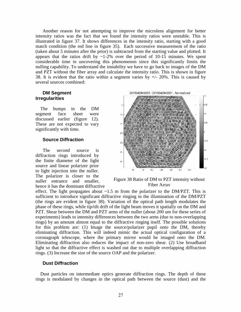
Another reason for not attempting to improve the microlens alignment for better intensity ratios was the fact that we found the intensity ratios were unstable. This is illustrated in figure 37. It shows differences in the intensity ratio, starting with a good match condition (the red line in figure 35). Each successive measurement of the ratio (taken about 5 minutes after the prior) is subtracted from the starting value and plotted. It appears that the ratios drift by ~1-2% over the period of 10-15 minutes. We spent considerable time in uncovering this phenomenon since this significantly limits the nulling capability. To understand the instability we have to go back to images of the DM and PZT without the fiber array and calculate the intensity ratio. This is shown in figure 38. It is evident that the ratio within a segment varies by +/- 20%. This is caused by several sources combined:

DM Segment Irregularities

The bumps in the DM segment face sheet were discussed earlier (figure 12). These are not expected to vary significantly with time. Source Diffraction

The second source is diffraction rings introduced by the finite diameter of the light source and linear polarizer prior to light injection into the nuller. The polarizer is closer to the nuller entrance and smaller, hence it has the dominant diffractive effect. The light propagates about ~1.5 m from the polarizer to the DM/PZT. This is sufficient to introduce significant diffractive ringing in the illumination of the DM/PZT (the rings are evident in figure 38). Variation of the optical path length modulates the phase of these rings, while tip/tilt drift of the light beam moves it spatially on the DM and PZT. Shear between the DM and PZT arms of the nuller (about 200 um for these series of experiments) leads to intensity differences between the two arms (due to non-overlapping rings) by an amount almost equal to the diffractive ringing itself. The possible solutions for this problem are: (1) Image the source/polarizer pupil onto the DM, thereby eliminating diffraction. This will indeed mimic the actual optical configuration of a coronagraph telescope, where the primary mirror would be imaged onto the DM. Eliminating diffraction also reduces the impact of non-zero shear. (2) Use broadband light so that the diffractive effect is washed out due to multiple overlapping diffraction rings. (3) Increase the size of the source OAP and the polarizer. Dust Diffraction

Dust particles on intermediate optics generate diffraction rings. The depth of these rings is modulated by changes in the optical path between the source (dust) and the

Figure 38 Ratio of DM to PZT intensity without

Fiber Array

28

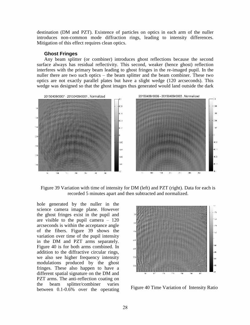
destination (DM and PZT). Existence of particles on optics in each arm of the nuller introduces non-common mode diffraction rings, leading to intensity differences. Mitigation of this effect requires clean optics. Ghost Fringes

Any beam splitter (or combiner) introduces ghost reflections because the second surface always has residual reflectivity. This second, weaker (hence ghost) reflection interferes with the primary beam leading to ghost fringes in the re-imaged pupil. In the nuller there are two such optics – the beam splitter and the beam combiner. These two optics are not exactly parallel plates but have a slight wedge (120 arcseconds). This wedge was designed so that the ghost images thus generated would land outside the dark

hole generated by the nuller in the science camera image plane. However the ghost fringes exist in the pupil and are visible to the pupil camera – 120 arcseconds is within the acceptance angle of the fibers. Figure 39 shows the variation over time of the pupil intensity in the DM and PZT arms separately. Figure 40 is for both arms combined. In addition to the diffractive circular rings, we also see higher frequency intensity modulations produced by the ghost fringes. These also happen to have a different spatial signature on the DM and PZT arms. The anti-reflection coating on the beam splitter/combiner varies between 0.1-0.6% over the operating Figure 40 Time Variation of Intensity Ratio

Figure 39 Variation with time of intensity for DM (left) and PZT (right). Data for each is

recorded 5 minutes apart and then subtracted and normalized.

29

bandpass of 650-800 nm (figure 50). At our experiment’s wavelength of 675 nm, it is 0.2%. Even this low reflectivity will produce ghost fringes with intensity modulation of ~18%. Reducing the modulation to 1% would require an anti-reflection coating with reflectivity = 0.000625%. While this is feasible at a single wavelength, a more practical solution is to use a broadband source such that the ghost fringes wash out, much like the diffraction affect.

Another option is to increase the wedge angle so that the ghost reflection is outside the acceptance cone of the fibers. The latter angle is 278 arcsec so that a wedge angle of ~3 times this, ~1000 arcsec would be required. However this larger wedge angle would introduce a glass thickness difference across the DM pupil equal to about 50 um. Control of dispersion (for broadband operation) requires that the glass thickness difference between the reflected and transmitted beams in the nuller should be less than 0.1 um. Therefore the beam splitter and combiner would need to be translated relative to each other with an accuracy of 20 um. This introduces another degree of freedom in the nuller that needs to be controlled, and while not impossible, it does complicate operation.

For future experiments we propose to follow several approaches – we will procure beam splitters with larger wedge angles and lower reflectivity in order to demonstrate narrow band performance, and then proceed to broadband experiments (but also see discussion for figure 42 below).

DM/PZT Tip/Tilt with respect to Fiber Array

The DM and PZT are imaged onto the Fiber Array face by an imaging relay. But there is no angle tracker to ensure that the DM and PZT maintain their angular orientation wrt the Fiber Array. Figure 41 shows the sensitivity of the Fiber Array output intensity to tip/tilt of the DM (it is very similar for the PZT). It is a simple derivative of figure 34. The sensitivity varies between +/- 0.2% per microradian of tip or tilt. The spatial variation between fibers occurs because of the clocking error discussed earlier. We know from other observations that the DM and PZT can drift wrt the Fiber Array by several microradians over 5-10 minutes depending on the thermal variation of the testbed – the testbed is in a small vacuum tank with no thermal control and is exposed to the variations of the ambient temperature. Hence drifts of several microradians are not surprising. This implies intensity variations of up to 1% level. Differential drift/sensitivity between the DM and PZT will then result in 0.1% level effects. The solution for this problem will be more stringent thermal control and less thermally sensitive design for all the optical mounts. An angle tracker may be needed if thermal control is insufficient.

In summary – several different sources combine to produce +/- 20% intensity fluctuations in the pupil prior to the Fiber Array. While some of the variation within segments is smoothed out by the spatial filtering during coupling of light into fibers, clearly there is a remnant effect at 1-2% that perturbs our intensity matching efforts and ultimately limits our null depth. The long term solutions for minimizing the impact of these issues are (1) pupil imaging of source/polarizer on to the DM, (2) cleaner optics, (3) better anti-reflection coatings larger wedge angle for the beam splitters, and (4) broadband operation. We were able to make a few measurement for #4 by measuring segment intensity ratios with broadband light (100 nm passband). Figure 42 shows the results. When compared to figure 37, we can see that intensity ratio fluctuations have been reduced by a factor of ~5 over similar time scales.

30

Figure 42 Intensity Ratio Variations for White Light

Figure 41 Fiber Coupling Sensitivity to Wavefront Tip/Tilt

31

Figure 44 Null Control Loop Example Figure 43 Three Successive Null Acquisition

Dither Sequences

4.2.4 Null Acquisition

Having matched intensities in the nuller as best as we can, we proceed to acquire the null by introducing a π phase shift between the two arms of the nuller. This is done initially by repeating the dither steps outlined previously and moving the PZT by half a wavelength and then the DM segments to achieve a near π phase shift. This process is not precise at the 50 pm level necessary for deeper nulls. So near the null position we change the control algorithm. We stop the dither steps and instead do a 3-point dither – at steps of -25 nm, 0 nm, and +25 nm around the starting null position. The output from the pupil camera for this dither sequence should look like a parabola, corresponding to the minimum location of a fringe where the ideal null is located. We record 2, 1, and 2 images at the dither locations. Figure 43 shows the values for a single pixel for 3 such dither sequences, showing the near parabolic variation. The parabola is fit for the location of the minimum and the resulting value is sent to the corresponding DM segment (after applying a 0.2 gain factor to reject noise). Figure 44 shows the performance of this control loop, whereby a starting offset of 1 nm is reduced to less than 100 pm. This data shows only one pixel. About 50 such pixels are averaged for each DM segment so the resulting accuracy is about 10 pm per control step.

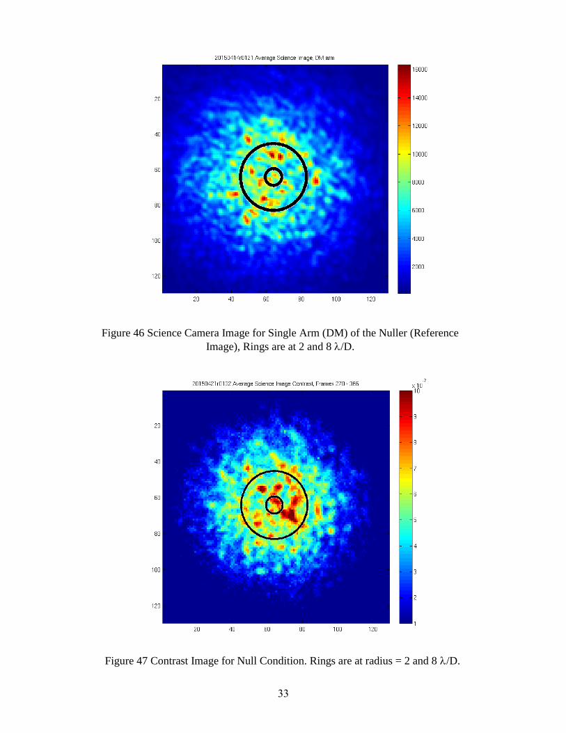
Once steady state has been achieved, we turn off the dither and record a series of images from the science camera. This comprises our null science data set. The dither sequence is then turned on for a few cycles and then turned off again to record science images. This on/off sequence can be repeated with flexibility, depending on the stability of the null. Figure 45 represents 4 such cycles. The plot displays the total science camera intensity, normalized to the input star light injection. Thus this plot shows how deeply we are able to null the total starlight intensity – about 2.5x10

-4. This is not contrast – that is

defined on a per pixel basis wrt the peak of the starlight point spread function (PSF). The PSF is displayed in figure 46. It does not look like an ideal coherent PSF because of the mismatch of the fibers in the Fiber Array. The Strehl ratio is very poor. It also does not look completely incoherent because the fiber lengths are within the coherence length of the laser. Here we should reiterate that the capability to null starlight is independent of the coherence of the Fiber Array output wavefront since our nulling algorithm works in the pupil plane. Thus all the data shown until now would look the same even if the array

32

was coherent. The only item that would change would be the PSF in the science camera. The degradation of the Strehl ratio with the current PSF will make it near impossible to detect a planet since its light would be distributed among the remnant starlight speckles.

The poor Strehl ratio makes it impossible to calculate a contrast ratio as used in traditional coronagraphy (speckle intensity at an off-axis pixel location divided by the PSF peak pixel value). Instead, we use a fraction of the total science image intensity as a proxy for the stellar PSF peak pixel intensity. We estimate this fraction to be in the range of one-third to one-tenth. This estimate is based on calculating the fractional energy contained in the peak pixel of an ideal Strehl ratio PSF and also agrees with the observation that the speckles in figure 46 and 47 appear to occupy between 3 to 10 pixels. The expected contrast ratio then equals the nulled science image divided by one-third to one-tenth of the total intensity of the single arm science image data. Figure 47 shows this science image contrast for a factor of one-tenth. The rings are at 2 and 8 /D radius. The mean contrast value in this range is 6x10

-7 (corresponding contrast using a factor of

one-third is 2x10-7

). The contrast is not dependent on radius because of the poor Strehl ratio. Figure 48 is a histogram of all the pixels within 2-8 /D (for a factor of one-tenth).

Figure 45 Science Camera Total Intensity during Null control loop

33

Figure 46 Science Camera Image for Single Arm (DM) of the Nuller (Reference

Image), Rings are at 2 and 8 /D.

Figure 47 Contrast Image for Null Condition. Rings are at radius = 2 and 8 /D.

34

4.2.5 Post-Coronagraph Calibrator

Our TDEM proposal had included the implementation of the post-coronagraph calibrator. The significant performance issues with the first generation Fiber Array and the effort spent to fabricate a new Fiber Array did not leave us with adequate time and resources to implement the calibrator. The implementation concept was made even more difficult by the fact that with the long length (2 m) fibers we would need to create a matching fiber length in the calibrator in order to obtain a zero optical path length match. It would also not be useful with the incoherent array since there is no unique path length to match. This problem is best solved by fabricating a matching length fiber at the same time as when we fabricate a new coherent array. We will address this issue in future experiments.

4.2.6 Discussion

Figure 45 indicates that our Null (in total intensity) is about 2.5x10-4

. The intensity ratio in figure 35 with rms = 0.8% would have implied a Null = 4x10

-6 (equation 1). We

know that the intensity ratio varies over time (figure 36) and degrades to about rms = 2%, implying a Null = 2.5x10

-5. So our Null is worse than predicted by a factor of 10.

However the estimated contrast of 6x10-7

is close to what we would predict using the measured Null: 2.5x10

-4/200 = 1.3x10

-6 (i.e. Null ratio divided by number of fibers).

Figure 48 Histogram of Science Image Contrast Values within 2-8 /D.

35

There are a few possibilities for the discrepancy between the predicted and measured Null:

(1) The intensity ratio is worse than rms = 2%. Null = 2.5x10-4

requires rms = 6%. We have not seen the intensity ratio degrade to that level in any of our measurements. It is however possible and will require a more thorough investigation.

(2) The intensity ratio we measure is not the actual intensity ratio if we do not measure all of the light in the fibers. For e.g. some pixels in the pupil camera are ignored. Since the fibers are single mode the output light distribution should be the same for both arms of the nuller. Missing a pixel from both arms should be a common mode effect that does not change the ratio measurement.

(3) The wavefront sensor camera is missing some of the light that reaches the science camera. For e.g. the imaging relay for the pupil camera does not capture all the light from the Fiber Array if some of the fibers’ light is angled outside the capture cone of the imaging relay. Another possibility is diffraction from the finite diameter of the microlenses. We suspect that this diffraction occurs but have not had time to investigate its effects.

(4) Phase offset between the two arms is not well controlled. Null = 2.5x10-4

requires phase error rms = 2 nm. Our measurements indicate that the phase is well controlled to less than 50 pm.

(5) The polarization state from the two arms of the nuller is not properly matched in the fibers. Our preliminary measurements of the polarization state of the Fiber Array output indicate that there is an effect at the 5-10% level – i.e. light from the two arms of the nuller displays different polarization state in the output beam (Figure 49). This is happening despite the existence of a linear polarizer for the input beam of the nuller. Lack of time has limited further investigation of this phenomenon.

We believe that the 3

rd and 5

th items hold the most promise to discover the reasons for

the worse than expected Null depth. While we have not met the Milestone that was agreed upon in the White paper, we

believe we have made significant progress in the state of the art of nulling coronagraphy using an array of single mode fibers. We have integrated an array of 200 fibers with a nulling interferometer and demonstrated phase and intensity control of light independently in all the individual fibers. The intensity matching experiments have already uncovered some significant limitations in the experimental setup (and perhaps polarization effects in the Fiber Array). These limitations need to be understood and reduced before we can proceed with fabrication of a coherent array. We did fabricate a smaller coherent fiber array as a proof of concept but it is yet to be tested. We plan to address these issues in future TDEM work.

36

Figure 49 Ratio of output beams (DM/PZT) with linear polarizer inserted in output beam.

4.3. Future Work

We have discussed many of the technical limitations to our current progress in the

previous section. Here we outline them in brief in order to present a cohesive picture of

our future efforts to improve the contrast ratio:

1. Intensity Ratio Stability – the stability of the intensity ratio is necessary for

achieving and maintaining deep nulls. We will procure a new beam splitter and

combiner pair with (1) very low anti-reflection coating for monochromatic

nulling, and (2) larger wedge angle. We will have to conduct a vendor survey to

discover the limitations for anti-reflection coating performance. It is likely that

the levels required (section 4.2.3, p. 29) will not be possible from commercial

sources (at least with a TDEM budget). We will have to proceed to broadband

operation to really overcome the ghost reflection problem. We do not foresee any

problems with this approach.

2. Fiber Array– The fiber array poses some serious technical challenges, chiefly

coherence and polarization. We have already explored many possible solutions to

solve the coherence problem and have described our initial effort to build a

coherent array (and its limitations) in 4.1.3, p. 19. We will need to measure the

performance of this array to gauge the effectiveness of our current technique. We

do not expect that the array will be sufficiently coherent due to fabrication

limitations. Our plan is to measure the path length differences between the fibers

in-situ once installed in the VNC and then fabricate a static compensation optic

37

fabricated from a fused silica plate that is etched to the desired path length depths

at JPL’s microdevices laboratory. Afterwards we will have to measure the

stability of the coherence to determine if an adaptive approach is required, i.e. a

post-coronagraph DM that would be set to compensate fiber path length

differences at whatever frequency is necessary. Adequate thermal control of the

testbed should assure that this would be a very low-frequency adjustment.

The polarization of the fiber array presents two different problems – (1)

polarization matching of the input beams within each fiber, and (2) polarization

matching of the output beams between all the fibers. The first is required for deep

nulls and the second is required for a good Strehl ratio PSF of the planet light.

Unfortunately we were not able to explore these two aspects in great depth during

this TDEM. Figure 49 is a preliminary data set exploring issue 1 (polarization

match within each fiber). It shows mismatch at the 5-10% level. This is currently

a mystery and needs further investigation. We need to measure the fiber input

light polarization ratio and compare with the output ratio. This is not an easy task

since it necessitates removal of the fiber array from the optical path so that the

pupil camera can image the light without the fiber array. The mismatch might be

in the input light or it might be influenced by the microlenses or the fibers. There

are many variables and it is not easy to separate them out.

The issue of polarization match between fibers is a function of the fabrication

technique (do the fibers get differentially twisted, or differential stress and

strain), and differential mechanical positioning of the fibers after installation –

i.e. if the fibers are in a loop on the optical bench then some might twist the

polarizations differently than other fibers. We need more experimental data to

quantify these problems. We note that the polarization issues can be explored

with the incoherent array alone, without having to resort to building a coherent

array.

It is possible that the long length fiber array will prove inadequate for nulling

for the above mentioned limitations. There are two alternative approaches that

would be possible – (1) a vendor (Luminit) has constructed a coherent array as

part of a NASA SBIR grant. They used photonic fabrication techniques to mass

produce waveguides at optical wavelengths and the desired spacing for the array.

It has not yet been evaluated for performance in a VNC (to check if it has similar

limitations as the short length fiber array), and (2) The VNC (without the fiber

array) can be configured to operate like an occulting mask coronagraph – the

nuller would be used to reject starlight and an electric-field conjugation (EFC)

algorithm (or equivalent) could be used to produce a dark hole. This is the

approach adopted by another VNC experiment (Lyon et. al. 2012). The latter

approach sacrifices the fiber array (which can yield a 360-degree dark hole) at the

expense of requiring a second DM if a 360-degree dark hole is necessary. It is not

yet clear whether the latter approach is suitable for segmented and obscured

aperture telescopes (which the fiber array handles easily).

38

4.4. Specifications of some Key Components

Figure 1 Anti-Reflection Coating performance of witness sample for nuller beam

splitter/combiner

Component Vendor Specifications

DM Boston Micromachines 331 segments

3 actuators per segment

Hexagonal pitch = 520 um

Quadratic motion law

Fiber Array (2nd

Gen, Incoherent)

Fiberguide Industries 331- Fibers, Type ASI4.3

Length 2 m +/- 2 mm

Fiber NA 0.12

Mode Field Diameter 4.5+/0.5 um

Microlenses JPL Microdevices

Laboratory

Diameter: 490 um

Lens Sag: 23 um

Focal Length: 3 mm

Substrate: Fused Silica

Materiel: SPR220-7

Spin Speed: 1200 rpm

39

Baked from 85 to 115 C

Developer AZ400K

Post-bake to 180 C for 1.5 hours

Linear Polarizer Newport 10LP-VIS-B

Diameter 25.4 mm

430-670 nm

Science Camera Andor CCD

256x256 pixel array

16 bit depth

Water cooled to 0 C

5-7 e read noise

0.5 Hz frame rate

Wavefront Sensor

Camera

Prosilica (Allied Vision) GB650 CMOS sensor

659x493 pixel array

10 Hz frame rate

Ambient temperature

5. References

Clampin, M., et. al., "Extrasolar Planetary Imaging Coronagraph (EPIC)", Proc. SPIE 6265, 2006.

Crepp, J. R., et. al., "Speckle Suppression with the Project 1640 Integral Field Spectrograph", ApJ, 729,132, 2011.

Guyon, O., "Imaging Faint Sources within a Speckle Halo with Synchronous Interferometric Speckle Subtraction", ApJ, 615, 562, (2004).

Hinkley, S., et. al., "A New High Contrast Imaging Program at Palomar Observatory", PASP, 123,74-86, 2011.

Lyon, R.G., Clampin, M., Woodruff, R.A., Vasudevan, G., Thompson, P., Petrone, P., Madison, T., Rizzo, M., Melnick, G., Tolls, V., "Visible nulling coronagraph testbed results", Proc. SPIE 7440, 744011 (2009).

Lyon, R.G., Clampin, M., Petrone, P., Mallik, U., Madison, T., Bolcar, M. R., "High Contrast Vacuum Nuller Tetsbed (VNT) Contrast, Performance and Null Control", Proc. SPIE 8442, 844208 (2012)

Postman, M., et. al., "ADVANCED TECHNOLOGY LARGE-APERTURE SPACE TELESCOPE (ATLAST): A TECHNOLOGY ROADMAP FOR THE NEXT DECADE", http://www.stsci.edu/institute/atlast/documents/ATLAST_NASA_ASMCS_Public_Report.pdf (Appendix K) (2009).

40

Pueyo, L., et. al., "Application of a Damped locally Optimized Combination of Images Method to the Spectral Characterization of Faint Companions Using an Integral Field Spectrograph", ApJ Supplement Series, 199, 6, 2012

Rao, S.R., Wallace, J. K., Samuele, R., Chakrabarti, S., Cook, T., Hicks, B., Jung, P., Lane, B., Levine, B.M., Mendillo, C., Schmidtlin, E., Shao, M., and Stewart, J., "Path length control in a nulling coronagraph with a MEMS deformable mirror and a calibration interferometer", Proc. SPIE 6888, 68880B (2008).

Samuele, R., Wallace, J. K., Schmidtlin, E., Shao, M., Levine, B. M., and Fregoso, S., "Experimental Progress and Results of a Visible Nulling Coronagraph", Aerospace Conference, 2007 IEEE , vol., no., pp.1-7, 3-10 March 2007.

Serabyn, E., “Nulling Interferometry: Symmetry Requirements and Experimental Results”, SPIE Vol 4006, 328-339, 2000.

Shao, M., et. al., "DAVINCI: Dilute Aperture Visible Nulling Coronagraphic Imager, ASTRO2010 Request for Information White Paper #36", http://sites.nationalacademies.org/BPA/BPA_049855, 2009

Trauger, J.T., Traub, W.A., "A laboratory demonstration of the capability to image an Earth-like extrasolar planet", Nature, 446, 771 (2007).

Vasisht, G., Crossfield, I.J., Dumont, P.J., Levine, B.M., Troy, M., Shao, M., Shelton, J.C. Wallace, J.K., "Post-Coronagraph Wavefront Sensing for the TMT Planet Formation Imager", Proc. SPIE 6272, 627253 (2006).

Wallace, J.K., Angione, J., Bartos, R., Best, P., Buruss, R., Fregoso, S., Levine, B.M., Nemati, B., Shao, M., Shelton, C., "Post-Coronagraph Wavefront Sensor for Gemini Planet Imager," Proc. SPIE 7015, 70156N (2008).

Wallace, J. K., Bartos, R., Rao, S., Samuele, R., Schmidtlin, E., "A Laboratory Experiment for Demonstrating Post-Coronagraph Wave Front Sensing and Control for Extreme Adaptive Optics," Proc. SPIE 6272, 62722L (2006).

Wallace, J.K., Macintosh, B., Shao, M., Bartos, R., Dumont, P., Levine, B.M., Rao, S., Samuele, R., Shelton, C., "An Interferometric Wave Front Sensor for Measuring Post-Coronagraph Errors on Large Optical Telescopes," Aerospace Conference, 2007 IEEE , vol., no., pp.1-7, 3-10 March 2007.

41

6. Acronyms

Acronym Explanation

APEP Visible Nuller Coronagraph testbed at

JPL

DAViNCI Dilute Aperture Visible Nulling

Coronagraphic Imager

DM Deformable mirror

EPIC Extrasolar Planetary Imaging

Coronagraph

IWA Inner Working Angle

OAP Off-Axis Parabola

VNC Visible Nulling Coronagraph