Technology Capital and the Taxation of Multinational

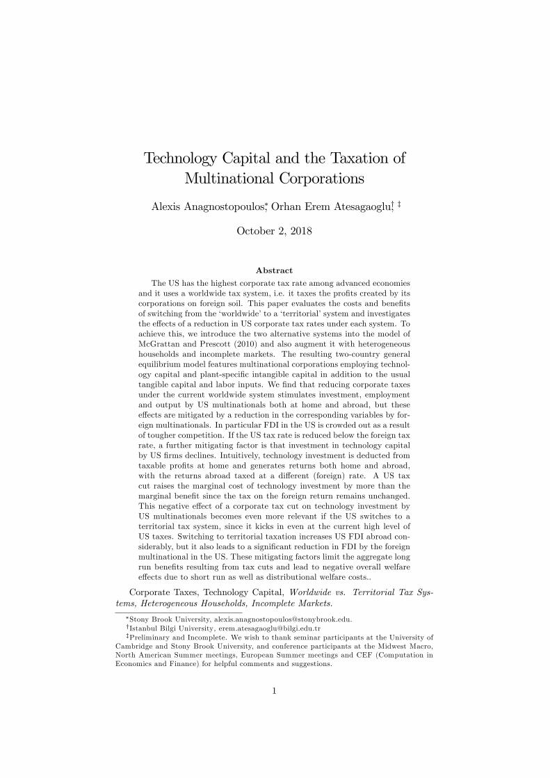
Technology Capital and the Taxation ofMultinational Corporations

Alexis Anagnostopoulos, Orhan Erem Atesagaogluy, z

October 2, 2018

Abstract

The US has the highest corporate tax rate among advanced economiesand it uses a worldwide tax system, i.e. it taxes the prots created by itscorporations on foreign soil. This paper evaluates the costs and benetsof switching from the worldwideto a territorialsystem and investigatesthe e¤ects of a reduction in US corporate tax rates under each system. Toachieve this, we introduce the two alternative systems into the model ofMcGrattan and Prescott (2010) and also augment it with heterogeneoushouseholds and incomplete markets. The resulting two-country generalequilibrium model features multinational corporations employing technol-ogy capital and plant-specic intangible capital in addition to the usualtangible capital and labor inputs. We nd that reducing corporate taxesunder the current worldwide system stimulates investment, employmentand output by US multinationals both at home and abroad, but thesee¤ects are mitigated by a reduction in the corresponding variables by for-eign multinationals. In particular FDI in the US is crowded out as a resultof tougher competition. If the US tax rate is reduced below the foreign taxrate, a further mitigating factor is that investment in technology capitalby US rms declines. Intuitively, technology investment is deducted fromtaxable prots at home and generates returns both home and abroad,with the returns abroad taxed at a di¤erent (foreign) rate. A US taxcut raises the marginal cost of technology investment by more than themarginal benet since the tax on the foreign return remains unchanged.This negative e¤ect of a corporate tax cut on technology investment byUS multinationals becomes even more relevant if the US switches to aterritorial tax system, since it kicks in even at the current high level ofUS taxes. Switching to territorial taxation increases US FDI abroad con-siderably, but it also leads to a signicant reduction in FDI by the foreignmultinational in the US. These mitigating factors limit the aggregate longrun benets resulting from tax cuts and lead to negative overall welfaree¤ects due to short run as well as distributional welfare costs..

Corporate Taxes, Technology Capital, Worldwide vs. Territorial Tax Sys-tems, Heterogeneous Households, Incomplete Markets.

Stony Brook University, [email protected] Bilgi University, [email protected] and Incomplete. We wish to thank seminar participants at the University of

Cambridge and Stony Brook University, and conference participants at the Midwest Macro,North American Summer meetings, European Summer meetings and CEF (Computation inEconomics and Finance) for helpful comments and suggestions.

1

1 Introduction

The United States currently possesses the highest statutory corporate income

tax rate among advanced economies, at 34 percent. It also stands alone among

advanced economies in taxing corporate income on a worldwide, as opposed

to a territorial, basis. Most countries tax only the profits earned within their

borders, i.e. they use a territorial tax system. In contrast, the US government

uses a worldwide system which means that, in addition to taxing the profits

earned within its borders, it also taxes the profits of US multinationals on their

operations in foreign countries.

In recent years, there have been several proposals for reforming the tax

system arising from a perceived bipartisan consensus that the US corporate tax

system needs to be fixed. In a joint report released by the White House and the

Department of the Treasury, President Obama’s framework for corporate tax

reform states that “America’s system of business taxation is in need of reform.”

and “...the tax reform...should properly balance the need to reduce tax incentives

to locate production overseas with the need for U.S. companies to be able to

compete overseas....”. In its conclusion, the report proposes to “...lower the

corporate tax rate to 28 percent, putting the United States in line with major

competitor countries...”. The proposal to reduce the corporate tax rate is in

line with several other reforms proposed. Examples include the “Bipartisan Tax

Fairness and Simplification Act (Wyden-Coats)” which proposes a flat rate of 24

percent, the “House Republican Tax Reform Plan (Dave Camp)” which calls for

a flat rate of 25 percent and the “National Commission on Fiscal Responsibility

and Reform (Bowles-Simpson)” suggesting a single tax rate between 23 and 29

percent. However, whereas the first two plans propose to maintain the current

worldwide tax system, the latter two plans aim to adopt a territorial tax system.

In favor of the worldwide system, President Obama’s framework states that

a “...territorial system could aggravate, rather than ameliorate, many of the

problems in the current tax code...firms would have even greater incentives to

locate operations abroad...”. The opposing view is that a territorial system will

increase the competitiveness of US corporations since they will face the same

tax rates as foreign competitors in foreign markets. Supporters of this view also

point to the fact that all major competitor countries are using a territorial tax

system and they have a lower tax rate.

This paper aims to contribute to the debate on corporate income taxation by

offering answers to the following questions: What are the costs and benefits of

switching from worldwide taxation to territorial taxation? How would a decrease

in corporate taxes affect domestic investment, FDI and employment in the US

under a worldwide tax system? How are these effects different under a territorial

tax system? Which US households would benefit and which would lose from

such changes? What would be the consequences of each proposed change for the

government’s budget and how do alternative ways of raising revenue compare

to each other?

In order to clarify and quantify the trade-offs involved, we build a multi-

country general equilibrium model which incorporates multinational corpora-

2

tions, heterogeneous households and incomplete markets. Each country has a

representative multinational firm that operates in all countries and a continuum

of households that are subject to uninsurable idiosyncratic income shocks. The

production technology follows closely McGrattan and Prescott (2010), where

firms use a constant returns to scale technology that combines four inputs of

production - labor, tangible capital, intangible capital and technology capital.

While multinationals make distinct investment decisions in each country for la-

bor, tangible and intangible capital, there is a single investment decision for

technology capital that affects both the home plant and the foreign plant of the

firm. In each country, households differ by labor earnings and wealth due to

uninsurable idiosyncratic income shocks as in Aiyagari (1994). Households sup-

ply labor and can invest in stocks and private international bonds which only

provide partial (self-) insurance against uncertainty. The government in each

country maintains a balanced budget and finances its expenditures by levying

taxes on labor income, dividends and corporate profits.

We find that incorporating technology capital is crucial for understanding the

effects of tax changes. Investment in technology capital yields returns both at

the home plant and abroad. In the benchmark calibrated economy, in which the

US government uses a worldwide tax system, US corporate taxes do not distort

technology capital. The reason is that technology investment is deductible from

taxable corporate profits. The marginal benefit of an increase in technology

capital comes from the sum of the after tax marginal products in the domestic

production plus the production abroad. Since both are taxed at the same rate,

this marginal benefit increases in proportion to the drop in the tax wedge when

the US corporate tax is reduced. The marginal cost, in the form of foregone

dividends, also increases in proportion to the tax wedge drop. As a result, the

tax does not distort technology capital. This, however, relies crucially on the

fact that the two marginal products are taxed at the same rate which is the case

because of the combination of two aspects of the tax code: first, the US tax rate

is higher than the foreign one and, second, the US system is a worldwide one.

Suppose the US switches to a territorial tax system without changing its tax

rate. The immediate implication is that the marginal product on the foreign

plant is now taxed at a lower rate and this renders the corporate tax distor-

tionary for technology capital. Notice, however, that the tax pushes technology

capital to a level higher than the undistorted one. The US corporation in-

vests additionally on technology capital to take advantage of the combination

of deductibility at home and lower tax on the return abroad. The exact oppo-

site situation is faced by the foreign multinational (even before the US switch)

which is subject to territorial taxation. Its investment in technology capital

is inefficiently low because part of its return, the one on US soil, is taxed at

a higher rate. Apart from the effects on technology capital, the US switch to

a territorial system induces the US multinational to increase tangible capital

investment abroad since it now faces the lower corporate tax rate on foreign

profits. So, overall US production abroad increases substantially but US pro-

duction at home also increases because higher technology capital also induces

the hiring of more inputs at home. However, the increase in home production of

3

the US multinational is significantly mitigated by the decrease in US production

of the foreign multinational which now faces higher input prices, i.e. wages and

bond returns. Thus, the US economy does not experience the large boom that

US corporations are experiencing because the growth of the US firm crowds out

foreign FDI in the US.

Interestingly, once the US has switched to a territorial taxation system, a de-

crease in the US corporate tax rate affects US technology investment negatively.

This is because the policy of investing in technology at home and receiving high

after tax returns abroad becomes less attractive as the home tax rate is reduced

and brought closer to the foreign tax rate. The result is that technology capital

falls at the same time that tangible capital increases. The technology capital

reduction dominates in the sense that it creates a reduction in other intangible

capital, in labor demand and in output by the US multinational at home. This

is one of the most striking results arising from our experiment, namely that

under a territorial tax system and in the presence of technology capital, a US

corporate tax cut reduces labor demand and output of the US multinational at

home.

Suppose now that the US maintains a worldwide tax system but reduces

the corporate income tax rate. The effects of this tax cut are more standard

for the US multinational which finds its after tax returns to tangible capital

increasing. As tangible capital increases, the returns to technology capital,

intangible capital and labor all increase and the US multinational increases its

production both at home and abroad. For the foreign multinational, the US tax

decrease implies increased incentives for technology investment. However, the

crowding out effect discussed above is too strong and the foreign multinational

reduces its investment and labor demand in the US. Overall, foreign FDI in the

US falls substantially and this largely undoes the increase in US output.

In sum, we identify two important mechanisms that render corporate tax

reform, whether in the form of lower rates or in the form of a switch to territorial

taxation, much less attractive than predicted in a standard growth model. First,

US multinationals can crowd out foreign multinationals implying a much smaller

increase in US output than expected. Second, lowering corporate taxes can have

negative effects on the investment and labor demand even of US multinationals

due to their effect on technology investment.

We also provide an assessment of the welfare consequences of the various

alternative reforms. We find both proposals, the switch to a territorial system

and the reduction in tax rates to be welfare reducing for two reasons: first,

because welfare costs associated with the short run drop in consumption domi-

nate the long run gains from higher consumption in the aggregate; second, the

corporate tax cut implies a redistribution of consumption from low wealth (high

marginal utility) households to high wealth (low marginal utility) households.

The latter "distributional" effect can be overturned by ensuring that the govern-

ment makes up for lost revenue from the corporate profits tax cut by increasing

dividend taxes as opposed to labor taxes. Even in those cases, social welfare

measures (based on a utilitarian welfare function) show an overall decrease in

social welfare.

4

Section 2 present the model and equilibrium definition, Section 3 discusses

the calibration and the results from our experiments and Section 4 concludes.

2 Model

Time is discrete and indexed by = 0 1 2 There are two countries in the

world economy. Each country has a representative multinational that operates

in both countries and a continuum of households that are subject to uninsurable

idiosyncratic income shocks. We start with the description of the production

technology and the maximization problem that multinationals face. We next

proceed with the description of the households’ optimization problem and the

government’s alternative budget constraints depending on whether it uses a

worldwide or territorial tax system. Finally, we provide the definition of equi-

librium for the model economy.

2.1 Firms

The production technology follows closely McGrattan and Prescott (2010). Each

country has a representative multinational that operates in both countries. The

output of multinational in country at time is represented by . In this

notation, the superscript = 1 2 is used to denote the country in which a

multinational firm is incorporated and the subscript = 1 2 is used to denote

the location of production. Accordingly, the total output in country is the

sum of the production of the home multinational = and the production of

the foreign multinational’s subsidiary 6= .

The output of multinational in country is produced by using four factors of

production: labor , tangible capital

, intangible capital

and technology

capital . Whereas labor, tangible capital and intangible capital are country

specific, technology capital is used at multiple locations simultaneously. In other

words, while multinationals invest in tangible and intangible capital in each

country, technology capital is accumulated only at the home country but used

in all foreign subsidiaries with no additional cost. Thus, from the perspective

of the foreign subsidiaries of a multinational, technology capital is a factor of

production that requires no foreign direct investment.

The output produced by multinational in its home country ( = ) is given

by

= (

), = 1 2 (1)

where denotes the total factor productivity of country and denotes the

population size of country .1 The production function () exhibits constant

returns to scale and is strictly increasing, strictly concave and satisfies the Inada

1Population size, together with technology capital, determines the number of locations

that a firm can use to open a plant in the country. See McGrattan and Prescott (2009) for a

detailed discussion of the microfoundations of the production function.

5

conditions. Similarly, the production of the foreign subsidiary of multinational

in country 6= is given by

= (

), = 1 2, 6= , (2)

where ∈ [0 1] denotes the degree of openness of country = 1 2 to foreign

direct investment. Note that the term represents the effective productivity

level that the foreign subsidiaries operating in country are subject to. If = 0,

this means country is closed to foreign direct investment. If = 1, domestic

and foreign corporations have the same productivity in country .

The capital stocks of multinationals evolve according to the following stan-

dard intertemporal accumulation equations,

=

+1 − (1− )

+Φ(

+1

) , = 1 2 (3)

=

+1 − (1− )

+Φ(

+1

) , = 1 2, = 1 2 (4)

=

+1 − (1− )

+Φ(

+1

) , = 1 2, = 1 2 (5)

where is investment in tangible capital,

is investment in intangible

capital, is investment in technology capital, is the depreciation rate

of technology capital, is the depreciation rate of tangible capital, is the

depreciation rate of intangible capital and Φ( ) denotes the capital adjustment

cost function.

The representative multinational incorporated in country maximizes the

discounted value of after-tax worldwide dividends,

∞X=0

2X=1

(1− ), (6)

where is the discount factor which is equal to the intertemporal price of

consumption, is the tax rate on total dividends paid out by multinational

, and denotes the dividends generated from operations in country . The

dividend payouts of multinational from domestic operations ( = ) and foreign

subsidiaries ( 6= ) are given respectively by

= (1− )

¡ −

−

−

¢+

−

(7)

= (1−

)³ −

−

´+

−

, 6= (8)

where is the corporate tax rate in country and 6= denotes the

corporate tax rate that multinational is subject to on its foreign profits. Note

that while intangible and technology capital investments are fully tax deductible,

corporations can deduct only the depreciation expenses for tangible capital. In

addition, recall that each multinational corporation invests in its technology

capital only at the home country, which is captured by the structure of cash

flow constraints (7) and (8).

6

Based on this setup, a multinational from country chooses sequences of

capital stocks and labor inputs to maximize the present discounted value of

after-tax dividends (6) subject to the cash flow constraints (7) - (8) and the

corresponding capital accumulation equations in (3) - (5).

2.2 Households

Each country has a continuum of households, of measure , indexed by

with identical preferences represented by the utility

0

∞X=0

() (9)

where is consumption of individual , in country at time , ∈ (0 1) is the

discount factor and 0 denotes the expectation conditional on information at

date = 0. The period utility function (·) is assumed to be strictly increasing,strictly concave and continuously differentiable.

Each household supplies a fixed amount of labor (normalized to one) and

receives a labor income of , where

denotes the idiosyncratic labor pro-

ductivity shock. The productivity shock is i.i.d. across households and follows

a Markov process with transition matrix Ω(0|). Households can also trade

financial assets and earn income from their asset holdings. More specifically, a

household in country can trade shares of the multinational with other

households in the country at the (ex-dividend) price .2 It can also trade a

bond internationally, with denoting the number of bonds bought at −1 and

denoting the corresponding gross return, which is deterministic since there

is no aggregate uncertainty. Households can use their after-tax labor and asset

incomes to purchase consumption goods and save. Their budget is given by

+

+

+1 = (1− )

+((1− )

¡1 +

2

¢+)

−1+

(10)

where and are the tax rates on dividends and labor income in country

at time . Households in each country are restricted to have positive wealth

(no-borrowing), i.e.

+

+1 ≥ 0 (11)

In the absence of aggregate uncertainty, the returns of the two assets are equal-

ized in equilibrium and the household’s composition of the portfolio between

shares and bonds is indeterminate. The household can be equivalently thought

of as choosing wealth ≡

+

+1 ≥ 0. International trade in bonds al-

lows the aggregate wealth in country to differ from the value of that coun-

try’s multinational corporation. It also implies equalization of stock returns,

2 It is well-known that there is a substantial bias in the data in favor of owning shares in

home corporations as opposed to foreign ones (see the large literature on the equity home bias

puzzle). Restricting households to buying only shares of the domestically incorporated firm

allows us to specify different dividend tax rates across countries.

7

and intertemporal marginal rates of substitution for unconstrained households,

across countries.

+1 =(1− )

¡1+1 +

2+1

¢+ +1

=

0 ()0

¡+1

¢ (12)

The value maximizing firm’s discount factor is simply = =0

0()0(0)

=

Y=0

1.

Each household chooses consumption and assets to maximize utility (9) sub-

ject to the budget constraint (10) and the no-borrowing constraint (11).

2.3 Government

In each country , the government consumes an exogenous, constant amount

which is financed by levying taxes on labor income, dividends and corporate

profits at rates and , respectively. Note that the corporate income

tax rates , 6= that a multinational corporation from country pays on

its foreign profits depend on whether the corporate income tax system in their

home country is a territorial or a worldwide system.

2.3.1 Territorial Taxation

Under a territorial tax system, country taxes only the profits earned within its

territory. In other words, country taxes the domestic profits of multinational

= and the profits of foreign subsidiaries operating in country at a tax rate

. In this system, a country does not tax the foreign profits earned by its

multinationals. Thus, the tax faced by a foreign subsidiary of a multinational

incorporated in country but operating in 6= is simply the foreign tax rate

= and the budget constraint of government is given by

= ¡1 +

2

¢+ + (Π

1 +Π

2) (13)

where = 1 + 2 denotes the total employment in country and Π1, Π2

denote the taxable profits of multinationals 1 and 2 respectively, from their

operations in country

Π = −

−

− −

, = 1 2

Π =

−

−

−

, = 1 2, 6=

2.3.2 Worldwide Taxation

Under a worldwide tax system, country taxes the profits earned within its

territory as well as the foreign profits earned by multinational = . In this

system, a country taxes its corporation’s total worldwide profits regardless of

the location of production. Notice that, if country adopts a worldwide tax

8

system, the foreign profits of multinational = would be taxed twice, first by

the country where the profits are generated and then a second time in its home

country . To avoid double taxation, country gives the multinational = a

tax credit for the foreign taxes that it has already paid. Based on this setup, the

effective tax rate that multinational is subject to on its foreign profits from

country 6= is = max . In terms of the government revenue, the

government in country receives tax revenue from these foreign profits only to

the extend that its tax rate is higher than the foreign tax rate, i.e. it receives

max − 0Π, 6= . The budget constraint of government is therefore

= ¡1 +

2

¢+ + (Π

1 +Π

2) + max − 0Π, 6= .

(14)

where Π denotes the taxable foreign profits of multinational

2.3.3 Summary for benchmark model

In our quantitative exercise we choose = 1 to denote the US and = 2 to denote

the rest of the world (ROW). Based on observed tax policies, we assume that

the ROW economy is under territorial tax system and the US economy is under

a worldwide tax system. In this case, the government budget for the US is given

by (14) and for the ROW by (13). The tax rate paid by US foreign subsidiaries

is 12 = max 1 2 and the one paid by ROW foreign subsidiaries in the US

is 21 = 1.

2.4 Competitive Equilibrium

Givenn©

ª2=1

12 21

o, initial capital stocks

½n

0

0

o2=1

0

¾2=1

and initial distributions of households 0 for each country , a competitive equi-

librium is a collection of household decision rules for consumption and wealth,

firms decision rules for labor, capital, investment and dividend distributions, ag-

gregate bond holdings in country , , laws of motion Γ for the cross-sectional

distribution in each country and prices , , such that:

(i) household decision rules solve the households’ maximization problems

given prices and dividends

(ii) firm decision rules solve the firms’ maximization problems given wages

and the discount factor =

Y=0

1

(iii) Markets clear. Specifically, the labor market in each country

= + =

Z for = 1 2, 6= (15)

the stock market in each countryR = 1 for = 1 2 (16)

9

the international bond market

2P=1

= 0 (17)

and goods’ market

2X=1

+

2X=1

+

2X=1

2X=1

h

+

i+

2X=1

=

2X=1

2X=1

(18)

where the are defined in equations (1) and (2).

(iv) The laws of motion Γ, = 1 2 are consistent with household decision

rules.

3 Quantitative Analysis

3.1 Calibration

The model is calibrated on an annual basis and the full set of parameters is

provided in Table 1. The momentary utility function of households has the

standard CRRA form

() =

()1− − 11−

(19)

with the coefficient of relative risk aversion set to one. The discount factor is

set to = 0948 so that the real interest rate is equal to 41%. The idiosyncratic

labor productivity process follows a parsimonious Markov chain with three states

and is taken from Domeij and Heathcote (2004).3 The productivity values

and the transition matrix Ω(+1

) are displayed in Table 2.

The production technology of multinational in country is represented by

the following Cobb-Douglas functional form

(

) = (

)

()

()

()

, = 1 2, = 1 2

(20)

with 0 1 and ++ + = 1, where , , and denote, respectively, the income shares of technology capital, intangible

capital, tangible capital and labor.

Technology parameters are chosen to match key features of the data taken

from Bureau of Economic Analysis (BEA) as in McGrattan and Prescott (2010).

The income share of labor is set to = 0651 to match the average labor

income share in the corporate sector over the post-war period. We use BEA

corporate sector data for the years 1980 - 2013 to calibrate and . The

tangible capital depreciation rate is set to = 006 to match the average

tangible investment to capital stock ratio of 006 and the income share of tangible

3The process is constructed so that it captures the autocorrelation and standard deviation

of the innovation of an AR(1) process estimated on US data as well as features of the cross-

sectional wealth inequality in US data.

10

capital is set to = 0214 to match the tangible capital to output ratio of

168. Following McGrattan and Prescott (2010) and Kapicka (2012), we set the

depreciation rate of technology capital to = 008, which is slightly lower than

the BEA’s estimates for depreciation of R&D investment.4 The income share

of technology capital and the depreciation rate for intangible capital are

calibrated jointly to match two moments: a technology capital investment rate

of 55 percent5 and a ‘market value-to-output ratio’ for the US corporate sector

over the period 2000-2014 of 2.35.6

The population size of US is normalized to one, 1 = 1. We restrict the

rest of the world economy to countries that have a significant FDI relationship

with the United States. We find that 19 countries receive 87% of US FDI and

that 93% foreign FDI in the US comes from those same countries.7 Accordingly,

the population size of the ROW economy is set to 2 = 24. Without loss of

generality, the TFP level of the US economy is normalized by setting 1 = 1.

Based on this normalization, we set 2 = 0698 to match the GDP of the rest

of the world economy relative to the US.

Recall that the extend to which countries are open to foreign direct in-

vestment is measured by the degree of openness parameters 1 2. We choose

2 = 0938 to match the US FDI position abroad as a share of domestic tangible

capital stock of US multinationals, which was 40 percent in 2013 based on the

BEA’s International Investment Position (IIP) data. Based on the same source

of data, we choose 1 = 0895 to match the FDI position in the US as a share

of the domestic tangible capital stock of US multinationals to be 25 percent.

Capital adjustment costs are commonly used in international macro models

to avoid excessive investment volatility and to capture the fact that financial

capital is more mobile than physical capital. In line with this, we assume that

tangible, intangible and technology capital investments are subject to a capital

adjustment cost that takes the form of Φ(+1

) = (

+1

− 1)2

following Mendoza, Quadrini and Rios-Rull (2007). We set the adjustment

cost parameter to = 06, which is the value used by Mendoza, Quadrini and

Rios-Rull (2007) and Kehoe and Perri (2002) to match the investment volatility

observed in the US and Europe. Note that, given the chosen functional form,

adjustment costs are irrelevant for the main steady state results discussed in the

following section.8

Finally, we choose tax rates for the US and ROW economies as follows.

4The BEA estimates that R&D investment depreciates at a rate of 11 precent annually.

See McGrattan and Prescott (2005) for details and further discussion.5This is obtained by McGrattan and Prescott (2010) from the BEA national income and

product accounts by classifying three types of investment as technology capital investment:

R&D expenditures, advertising expenditures and organization capital expenditures.6Based on our own calculations using NIPA and Flow of Funds Accounts.7The countries are the UK, Netherlands, Japan, Canada, France, Switzerland, Germany,

Luxemburg, UK Caribbean Islands, Belgium, Spain, Australia, Sweden, South Korea, Ireland,

Norway, Mexico, Italy, Singapore.8The parameterization of the cost function does affect the speed of adjustment to steady

state after a tax change and, as a result, can affect the quantitative results regarding welfare

effects. We conduct sensitivity analysis with respect to the parameter when discussing the

welfare results.

11

For the US economy, we set the dividend tax rate to 1 = 020 which is the

top statutory rate in effect since the American Taxpayer Relief Act of 2012.

We set the corporate income tax rate to 1 = 034 which is roughly equal to

the marginal statutory rate that US corporations are subject to. For the labor

income tax rate, we follow McGrattan and Prescott (2010) by setting 1 = 029.

For the ROW economy, since we restrict the rest of the world to countries

that have significant FDI relationship with the US, we can determine the average

corporate income tax rate by looking at the foreign tax credits that the IRS

affords to US corporations. Based on the IRS’ Statistics of Income (SOI) data,

we find that the effective tax rate that US corporations paid on their foreign

earned income was quite stable and roughly equal to 25% over the period 1992

- 2010. Accordingly, we set 2 = 025. For dividend and labor income tax

rates, we construct weighted averages using the statutory rates in 2013. With

the weights based on GDP of each country, we find that the weighted average

tax rates for dividend and labor income are equal to 2 = 016 and 2 = 035,

respectively.

3.2 Reducing the corporate income tax

Table 4A presents the long run effects on both the US and the ROW economy

of reducing the corporate tax rate in the US from 035 to several different levels

down to zero. Figure 1 provides a visual summary of the same effects focusing

on the three types of capital stock and output. The left panel of that figure

shows the effects on capital and output in the US and the right panel shows the

corresponding effects on the ROW.

It is clear from looking at the figures, that the effects of a corporate tax cuts

on aggregates hinge critically on whether the US tax is reduced to a level below

the tax rate in the ROW (025) or not. Specifically, aggregate variables increase

(decrease) with a reduction of the tax rate up to 0.25 but then start decreasing

(increasing) when the tax rate is reduced further below 025.

To explain the effects of the corporate tax cut it is helpful to clarify first

which margins are distorted by corporate taxes and this depends on the type

of system (worldwide vs territorial) that a multinational is subject to as well as

the relative size of the tax rate in the two countries.

Consider first the region where the US (worldwide system) tax rate is higher

than the ROW (territorial) tax rate, i.e. the experiments where 1 is reduced but

only up to 2 = 025. In this case, the US corporate tax directly distorts (i.e. it

affects the corresponding Euler equation) tangible capital investment for the US

multinational in both home and foreign plants and tangible capital investment

of the ROW multinational in its US plant. In contrast, it does not directly

distort intangible capital investment for any plant because this is deducted from

corporate taxation. The effect on technology investment is slightly more subtle

because technology investment yields two marginal products, one at the home

plant and one at the foreign plant. It is straightforward to see the effects of

corporate taxation by looking at the first order condition for technology capital

12

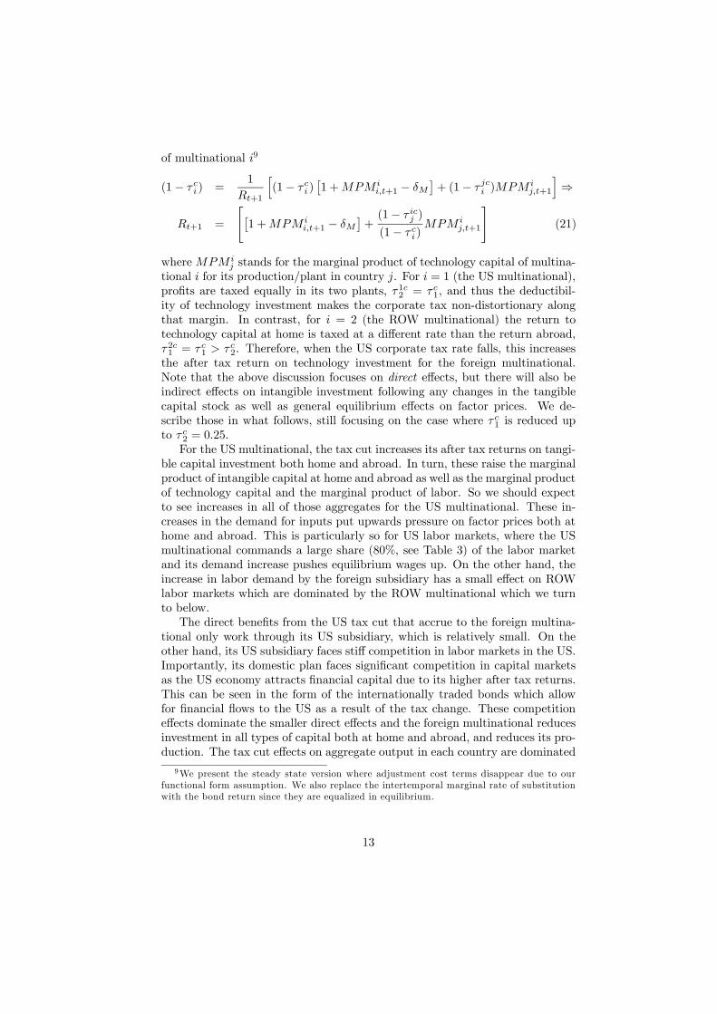
of multinational 9

(1− ) =1

+1

h(1− )

£1 +

+1 − ¤+ (1−

)

+1

i⇒

+1 =

"£1 +

+1 − ¤+(1− )

(1− )

+1

#(21)

where stands for the marginal product of technology capital of multina-

tional for its production/plant in country . For = 1 (the US multinational),

profits are taxed equally in its two plants, 12 = 1, and thus the deductibil-

ity of technology investment makes the corporate tax non-distortionary along

that margin. In contrast, for = 2 (the ROW multinational) the return to

technology capital at home is taxed at a different rate than the return abroad,

21 = 1 2. Therefore, when the US corporate tax rate falls, this increases

the after tax return on technology investment for the foreign multinational.

Note that the above discussion focuses on direct effects, but there will also be

indirect effects on intangible investment following any changes in the tangible

capital stock as well as general equilibrium effects on factor prices. We de-

scribe those in what follows, still focusing on the case where 1 is reduced up

to 2 = 025.

For the US multinational, the tax cut increases its after tax returns on tangi-

ble capital investment both home and abroad. In turn, these raise the marginal

product of intangible capital at home and abroad as well as the marginal product

of technology capital and the marginal product of labor. So we should expect

to see increases in all of those aggregates for the US multinational. These in-

creases in the demand for inputs put upwards pressure on factor prices both at

home and abroad. This is particularly so for US labor markets, where the US

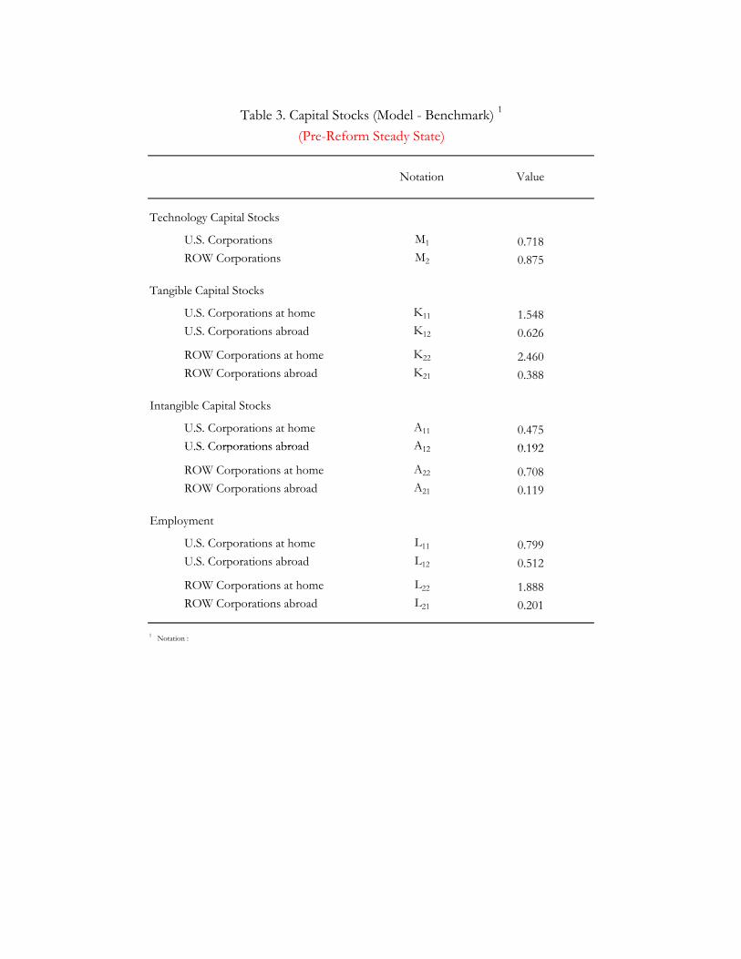
multinational commands a large share (80%, see Table 3) of the labor market

and its demand increase pushes equilibrium wages up. On the other hand, the

increase in labor demand by the foreign subsidiary has a small effect on ROW

labor markets which are dominated by the ROW multinational which we turn

to below.

The direct benefits from the US tax cut that accrue to the foreign multina-

tional only work through its US subsidiary, which is relatively small. On the

other hand, its US subsidiary faces stiff competition in labor markets in the US.

Importantly, its domestic plan faces significant competition in capital markets

as the US economy attracts financial capital due to its higher after tax returns.

This can be seen in the form of the internationally traded bonds which allow

for financial flows to the US as a result of the tax change. These competition

effects dominate the smaller direct effects and the foreign multinational reduces

investment in all types of capital both at home and abroad, and reduces its pro-

duction. The tax cut effects on aggregate output in each country are dominated

9We present the steady state version where adjustment cost terms disappear due to our

functional form assumption. We also replace the intertemporal marginal rate of substitution

with the bond return since they are equalized in equilibrium.

13

by the home multinational. As a result, aggregate output goes up in the US

and down in the ROW in the long run.

Before considering what happens when the US reduces the tax rate even fur-

ther below 025, we comment briefly on welfare effects. These are presented in

Table 4B (and Figure 5A). From an aggregate welfare perspective, we decompose

the effects on a utilitarian social welfare function in each country to aggregate

and distributional components, as in Domeij and Heathcote (2004). The ag-

gregate component simply captures the welfare consequences of the changes in

aggregate consumption along the path to the new steady state whereas the dis-

tributional component captures the effects of consumption redistribution across

households and is computed as a residual. Aggregate consumption in the US

increases in the long run but only at the cost of a short run investment boom

and consumption drop. The short run drop dominates quantitatively making

the overall path of aggregate consumption associated with welfare losses (see

Table 4B, US Aggregate Component). In the ROW, there is significant disin-

vestment in the short run which means aggregate consumption increases in the

short run. In addition, long run consumption is mostly unaffected (actually

increases slightly) so the overall consumption path is always higher than the

benchmark economy. As a result, the aggregate component of welfare goes up.

In both countries, after tax returns to capital increase whereas the after tax

wage decreases so, from a distributional perspective, welfare gains (losses) are

smaller (larger) for the poorest households who earn labor income and hold lit-

tle or no assets. This negative redistribution registers in Table 4B as a negative

distributional effect for our utilitarian social welfare function.

We now turn to the case where the US corporate tax rate is reduced fur-

ther below 025, making the US corporate tax rate lower than the foreign one.

It is interesting to note that most of the results discussed above are reversed

in the sense that many aggregate variables that increased (decreased) as the

US tax rate moved from 034 to 025 now do the exact opposite as the tax

rate moves from 025 to 0. This striking difference arises due to two impor-

tant changes in the effects discussed above. First, tangible capital investment

of the US multinational abroad is now taxed at the foreign rate (025) and the

decrease in the US rate no longer has a positive effect on that. Second, and

more importantly, the reduction in the corporate tax rate reduces the incen-

tives for technology investment by the US multinational. This might appear

counterintuitive at first glance, but it can be easily understood with reference

to the optimal choice of technology capital for = 1 described in equation (21).

Since 12 = max 1 2, this tax rate fell along with 1 as long as 1 ≥ 025,

but now remains fixed and equal to 2 = 025 as 1 falls. Intuitively, 1 was

not distortionary for values above 025 because the marginal cost and marginal

benefit of technology investment moved exactly proportionally with changes in

1. For values of 1 below 025, whereas the marginal cost keeps rising at the

same rate, the marginal benefit does no longer rise as fast because part of the

return, the one coming from the foreign plant, is taxed at the foreign rate which

does not fall.

Using these direct effects of the tax cuts, we can now explain the observed

14

movements in the aggregates. Starting with the US multinational at home,

the tax change tilts its choice of inputs towards more tangible capital and less

technology capital. In turn, the decrease in technology capital reduces the

marginal product of other all inputs in the foreign plant and, as a result, the

inputs and production by the foreign plant fall as the corporate tax rate falls

below 025 in the US. The ROW multinational now still has the direct benefits

of higher return to its foreign tangible capital as well as higher returns to its

technology capital. Contrary to before, it does not face a significant increase in

competition in either market. As a result its home production increases and its

US production increases by even more.

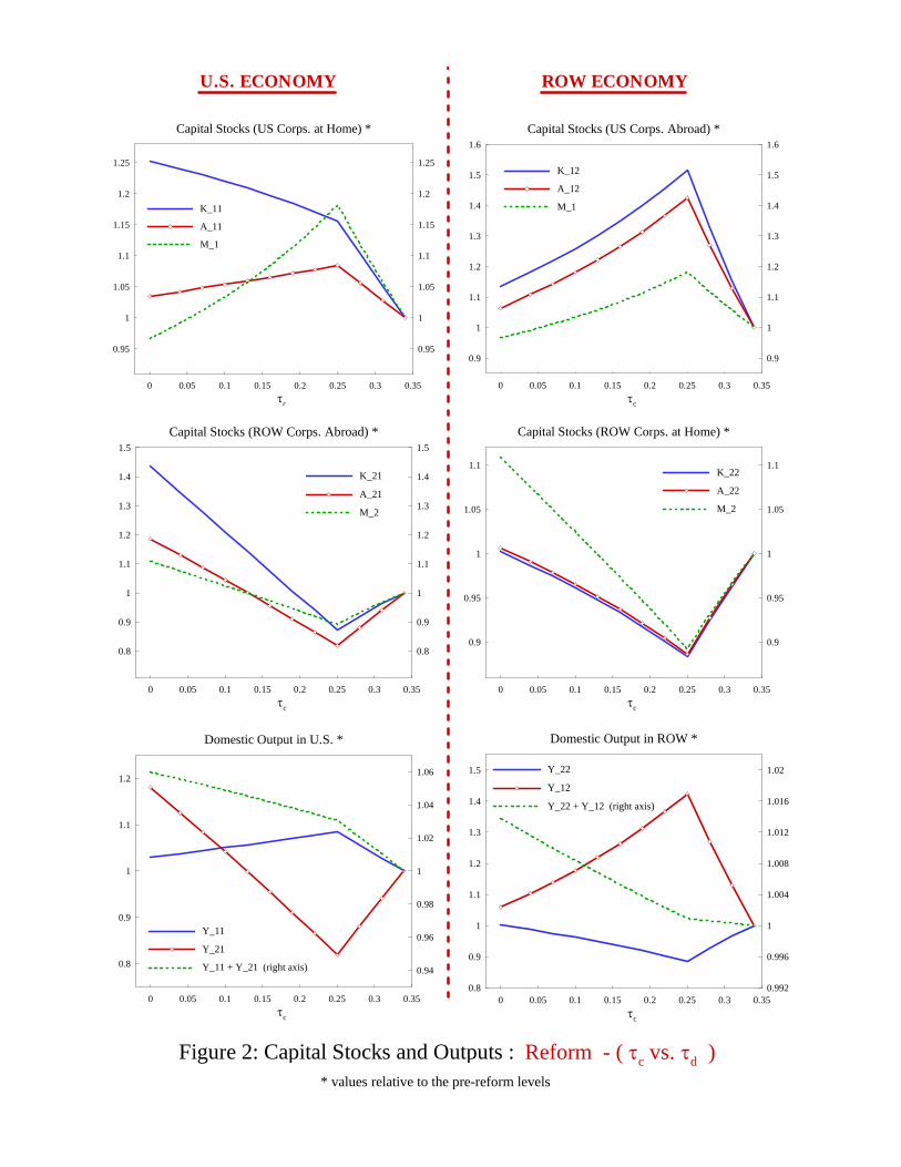
Tables 5A, 5B and Figure 2 present results for the same experiment with the

difference being that the government revenue shortfall arising from lower cor-

porate taxes is balanced by an increase in dividend taxes instead of labor taxes.

This alternative policy does not have significant differences from the benchmark

experiment with respect to long run aggregates. What it does achieve is to lead

to a more equitable distribution of consumption so that the distributional com-

ponent of social welfare in the US is now positive instead of negative. The

reason is that low wealth households, which earn income mainly from labor, do

not experience an increase in labor taxes anymore. Instead, it is wealthy house-

holds that now have to pay higher dividend taxes. As a result, consumption

is redistributed towards the bottom of the consumption distribution, the dis-

tributional component of welfare increases (due to the utilitarian social welfare

function employed) and overall social welfare losses are mitigated relative to the

benchmark experiment.

3.3 Switching from Worlwide to Territorial System

An alternative approach to corporate tax reform that is often suggested (see

discussion in the Introduction) is for the US to change its system of corporate

taxation from a worldwide system to a territorial one, conforming to the system

followed by the majority of OECD countries. A change in the system will change

effective tax rates for US multinationals even if there is no change in the chosen

tax rate, since the profits from foreign operations of US multinationals will now

be taxed at the foreign tax rate. It will also change the revenues collected by

the US government, essentially taking away its revenues from the profits of US

subsidiaries abroad. We conduct this alternative experiment below and present

the results in Tables 6A, 6B, and Figure 3 (Tables 7A, 7B and Figure 4 for the

case where dividend taxes are used to balance the budget).

Notice that any tax change that brings the US corporate tax rate at or below

the foreign rate (025) has the same effect regardless of whether the US follows

a worldwide or territorial system. This is because the US subsidiaries abroad

necessarily face the local tax and, if the US tax rate were lower, there would

be nothing left for the US government to collect after tax credits are applied.

Hence, our discussion focuses on the interesting part where the US switches to

a territorial system and either maintains the tax rate of 034 or simultaneously

reduces the tax rate up to 025.

15

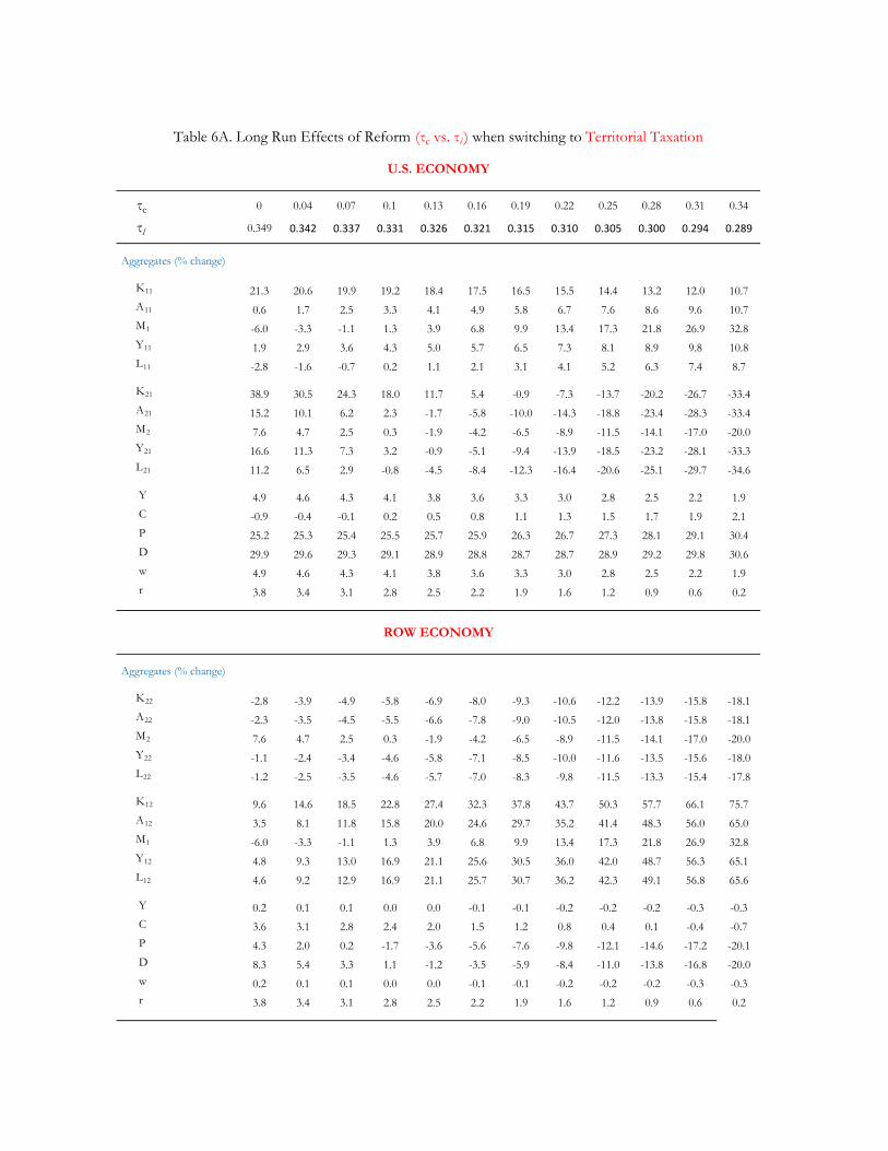
Consider first a switch to territorial taxation with no change in the tax rate.

The direct effect of such a change comes from the change in the effective tax rate

that the US multinational faces on its profits abroad, i.e. 12 falls abruptly from

034 to 025. As explained earlier, this affects the return to tangible capital in the

foreign plant and it also affects the return to technology capital. Thus, both12

and 1 rise by a significant amount. The increase in technology capital pushes

other inputs in the domestic plant upwards. For the foreign plant, inputs rise

even more strongly because the technology capital increase is combined with an

increase in tangible capital, making the marginal product of intangible capital

and of labor rise by a large amount. On the other hand, the foreign corporation

still faces the same tax rate at its US plant but now faces stiffer competition

in both labor markets as well as the capital market. With wages and returns

rising, the foreign multinational reduces its production in both of its plants.

Once the US has switched to a territorial system, a decrease in the tax rate

now creates disincentives for technology capital investment by the US multi-

national. The intuition is again that the marginal cost of investment is rising

faster than the marginal benefit, since part of the benefit comes from the foreign

plant profits and the tax on those remains fixed at the ROW tax rate. As a

result, decreases in the US corporate tax rate under a territorial system tilt the

incentives for investment away from technology capital and towards tangible

capital in the US. Quantitatively, the technology capital reduction dominates

and leads to decreases in intangible capital, labor and output at both the home

and foreign plants of the US multinational. In turn, this reduces the pressure on

the ROW multinational and increases its production. In a nutshell, the pattern

of effects arising from a US tax cut when the US is already on a territorial sys-

tem follows qualitatively the one observed when the US tax rate is lower than

the ROW rate under a worldwide US system.

4 Conclusion

Taking into account technology capital and carefully distinguishing between

worldwide and territorial tax systems are found to be important for evaluating

corporate tax policy. Macroeconomic models typically abstract from these as-

pects and this paper has filled this gap in the literature. Long run effects on

US GDP from switching to a territorial tax system can be positive because US

multinationals will face lower taxes on their foreign profits which induces them

to invest more in technology and this, in turn, feeds back to higher (tangible)

capital and labor demand at home. Once the switch has been established, de-

creases in the tax rate actually have a negative effect on technology investment

incentives for US multinationals. However, foreign multinational investment in

the US benefits from such a decrease and as a result US production still increases

in the long run.

The effects of corporate tax cuts on technology investment can be very dif-

ferent if the US maintains a worldwide tax system. In that case, a tax cut

can increase US technology investment through an indirect effect, namely by

16

increasing the returns to tangible investment and, as a result of this, the mar-

ginal product of technology investment too. The negative effects of tax cuts

on technology can arise also under a worldwide system, if the US tax rate is

reduced to the extent that it becomes lower than foreign corporate tax rates.

Finally, despite potential benefits from tax cuts in terms of long run pro-

duction, our model corroborates the results in a growing literature10 that finds

negative welfare effects of such tax cuts when the transitional and distributional

costs of such a change are taken into account.

10See Domeij and Heathcote (2004) and Anagnostopoulos, Carceles-Poveda and Lin (2012)

and the references therein.

17

References

[1] Aiyagari, D. R., 1994. "Uninsured Idiosyncratic Risk and Aggregate Saving."

Quarterly Journal of Economics 109 (3), pp. 659-684.

[2] Anagnostopoulos, A., Carceles-Poveda, E., Lin, D., 2012. "Dividend and

Capital Gains Taxation under Incomplete Markets" Journal of Monetary

Economics, 59 (7), pp. 898-919.

[3] Domeij, D., Heathcote, J., 2004. "On the Distributional Effects of Reducing

Capital Taxes." International Economic Review, 45 (2), pp. 523-554.

[4] Kapicka, M., 2012. "How Important is Technology Capital for the United

States?" American Economic Journal: Macroeconomics, 4 (2), pp. 218-248.

[5] Kehoe, P.J., Perri, F., 2002. "International Business Cycles with Endogenous

Incomplete Markets." Econometrica, 70(3), 907-928.

[6] McGrattan, E.R., Prescott, E.C., 2010. "Technology Capital and the US

Current Account." American Economic Review, 100 (4), pp. 1493-1522.

[7] McGrattan, E.R., Prescott, E.C., 2009. "Openness, Technology Capital, and

Development." Journal of Economic Theory, 144, pp. 2454-2476.

[8] McGrattan, E.R., Prescott, E.C., 2005. "Taxes, Regulations, and the Value

of US and UK Corporations." Review of Economic Studies, 72, pp. 767-796.

[9] Mendoza, E., Quadrini, V., Rios-Rull, V., 2007. "On the Welfare Impli-

cations of Financial Globalization without Financial Development." NBER

International Seminar on Macroeconomics.

18

Parameter Value

Discount Factor β 0.948Share of Technology Capital in Production α m 0.070Share of Intangible Capital in Production α a 0.065Share of Tangible Capital in Production α k 0.214Share of Labor in Production α l 0.651Depreciation Rate - Technology Capital δ m 0.080Depreciation Rate - Intangible Capital δ a 0.080Depreciation Rate - Tangible Capital δ k 0.060CRRA Parameter µ 1.00Adjustment Cost ψ 0.60Labor Productivity Shocks ϵ it See Table 2Tax Rate on Corporate Income - US τ c1 0.34Tax Rate on Corporate Income - ROW τ c2 0.25Tax Rate on Dividends - US τ d1 0.20Tax Rate on Dividends - ROW τ d2 0.16Tax Rate on Labor Income - US τ l1 0.29Tax Rate on Labor Income - ROW τ l2 0.35TFP - US Z 1 1.000TFP - ROW Z 2 0.698Population - US N 1 1.00Population - ROW N 2 2.40Openness - US σ 21 0.895Openness - ROW σ 12 0.938

Table 1. Common Parameter Values - Baseline Calibration

1964-1983 1984-2004

Data Model Data Model

Debt / GDP 0.607 0.575 0.805 0.725

Tobin's q (V/k) 0.665 0.748 0.929 0.932

Table 2: Corporate Debt and Equity Markets - Period Averages (τc-constant)

0.167 0.839 5.087

0.900 0.100 0.000

Table 2. Labor Productivity Process *

є =

0.005 0.990 0.0050.000 0.100 0.900

and Ω(є'/є) is the Markov transition matrix.

Ω(є'/є) =

* Notation: є denotes the values of the labor productivity shock,

1964-1983 1984-2004


Debt / GDP 0.607 0.575 0.805 0.725

Tobin's q (V/k) 0.665 0.748 0.929 0.932

Table 2: Corporate Debt and Equity Markets - Period Averages (τc-constant)1964-1983 1984-2004


Debt / GDP 0.607 0.575 0.805 0.725

Tobin's q (V/k) 0.665 0.748 0.929 0.932


1964-1983 1984-2004


Debt / GDP 0.607 0.575 0.805 0.725

Tobin's q (V/k) 0.665 0.748 0.929 0.932


Notation Value

Technology Capital Stocks

U.S. Corporations M1 0.718 ROW Corporations M2 0.875

Table 3. Capital Stocks (Model - Benchmark) 1

(Pre-Reform Steady State)

Tangible Capital Stocks

U.S. Corporations at home K11 1.548 U.S. Corporations abroad K12 0.626

ROW Corporations at home K22 2.460 ROW Corporations abroad K21 0.388

Intangible Capital Stocks

U.S. Corporations at home A11 0.475U S Corporations abroad A12 0 192 U.S. Corporations abroad A12 0.192

ROW Corporations at home A22 0.708 ROW Corporations abroad A21 0.119

Employment

U.S. Corporations at home L11 0.799 U.S. Corporations abroad L12 0.512

ROW Corporations at home L22 1.888 ROW Corporations abroad L21 0.201

1 Notation :

1964-1983 1984-2004


Debt / GDP 0.607 0.575 0.805 0.725

Tobin's q (V/k) 0.665 0.748 0.929 0.932


τc 0 0.04 0.07 0.1 0.13 0.16 0.19 0.22 0.25 0.28 0.31 0.34

τl 0.349 0.342 0.337 0.331 0.326 0.321 0.315 0.310 0.305 0.300 0.295 0.290

Aggregates (% change)

K11 21.3 20.6 19.9 19.2 18.4 17.5 16.5 15.5 14.4 9.6 4.8 - A11 0.6 1.7 2.5 3.3 4.1 4.9 5.8 6.7 7.6 5.1 2.5 - M1 -6.0 -3.3 -1.1 1.3 3.9 6.8 9.9 13.4 17.3 11.2 5.4 - Y11 1.9 2.9 3.6 4.3 5.0 5.7 6.5 7.3 8.1 5.4 2.7 - L11 -2.8 -1.6 -0.7 0.2 1.1 2.1 3.1 4.1 5.2 3.4 1.7

K21 38.9 30.5 24.3 18.0 11.7 5.4 -0.9 -7.3 -13.7 -8.6 -4.0 - A21 15.2 10.1 6.2 2.3 -1.7 -5.8 -10.0 -14.3 -18.8 -12.3 -6.1 - M2 7.6 4.7 2.5 0.3 -1.9 -4.2 -6.5 -8.9 -11.5 -7.2 -3.4 - Y21 16.6 11.3 7.3 3.2 -0.9 -5.1 -9.4 -13.9 -18.5 -12.1 -5.9 - L21 11.2 6.5 2.9 -0.8 -4.5 -8.4 -12.3 -16.4 -20.6 -13.7 -6.8

Y 4.9 4.6 4.3 4.1 3.8 3.6 3.3 3.0 2.8 1.9 0.9 -

C -0.9 -0.4 -0.1 0.2 0.5 0.8 1.1 1.3 1.5 1.0 0.5 -

P 25.2 25.3 25.4 25.5 25.7 25.9 26.3 26.7 27.3 17.6 8.5 -

D 29.9 29.6 29.3 29.1 28.9 28.8 28.7 28.7 28.9 18.5 8.9 -

w 4.9 4.6 4.3 4.1 3.8 3.6 3.3 3.0 2.8 1.9 0.9 -

r 3.8 3.4 3.1 2.8 2.5 2.2 1.9 1.6 1.2 0.8 0.4 -


K22 -2.8 -3.9 -4.9 -5.8 -6.9 -8.0 -9.3 -10.6 -12.2 -7.8 -3.7 - A22 -2.3 -3.5 -4.5 -5.5 -6.6 -7.8 -9.0 -10.5 -12.0 -7.7 -3.7 - M2 7.6 4.7 2.5 0.3 -1.9 -4.2 -6.5 -8.9 -11.5 -7.2 -3.4 - Y22 -1.1 -2.4 -3.4 -4.6 -5.8 -7.1 -8.5 -10.0 -11.6 -7.4 -3.5 - L22 -1.2 -2.5 -3.5 -4.6 -5.7 -7.0 -8.3 -9.8 -11.5 -7.3 -3.5

K12 9.6 14.6 18.5 22.8 27.4 32.3 37.8 43.7 50.3 31.8 15.0 - A12 3.5 8.1 11.8 15.8 20.0 24.6 29.7 35.2 41.4 26.3 12.6 - M1 -6.0 -3.3 -1.1 1.3 3.9 6.8 9.9 13.4 17.3 11.2 5.4 - Y12 4.8 9.3 13.0 16.9 21.1 25.6 30.5 36.0 42.0 26.7 12.7 - L12 4.6 9.2 12.9 16.9 21.1 25.7 30.7 36.2 42.3 26.9 12.8

Y 0.2 0.1 0.1 0.0 0.0 -0.1 -0.1 -0.2 -0.2 -0.1 -0.1 -

C 3.6 3.1 2.8 2.4 2.0 1.5 1.2 0.8 0.4 0.3 0.1 -

P 4.3 2.0 0.2 -1.7 -3.6 -5.6 -7.6 -9.8 -12.1 -7.7 -3.7 -

D 8.3 5.4 3.3 1.1 -1.2 -3.5 -5.9 -8.4 -11.0 -6.9 -3.3 -

w 0.2 0.1 0.1 0.0 0.0 -0.1 -0.1 -0.2 -0.2 -0.1 -0.1 -

r 3.8 3.4 3.1 2.8 2.5 2.2 1.9 1.6 1.2 0.8 0.4 -

Table 4A. Long Run Effects of Reform (τc vs. τl )

U.S. ECONOMY

ROW ECONOMY

τc 0 0.04 0.07 0.1 0.13 0.16 0.19 0.22 0.25 0.28 0.31 0.34

τl 0.349 0.342 0.337 0.331 0.326 0.321 0.315 0.310 0.305 0.300 0.295 0.290

Welfare (%) -3.34 -2.88 -2.54 -2.23 -1.93 -1.66 -1.40 -1.18 -0.99 -0.61 -0.28 -

Aggregare Component (%) -1.25 -1.02 -0.86 -0.71 -0.58 -0.47 -0.38 -0.31 -0.26 -0.14 -0.05 -

Distributional Component (%) -2.12 -1.88 -1.70 -1.53 -1.36 -1.19 -1.03 -0.88 -0.73 -0.47 -0.24 -

Welfare (%) 0.40 0.35 0.32 0.30 0.28 0.26 0.25 0.25 0.25 0.16 0.08 -

Aggregare Component (%) 0.77 0.68 0.62 0.56 0.50 0.45 0.40 0.35 0.31 0.21 0.10 -


Table 4B. Welfare Gains : Reform (τc vs. τl )

U.S. ECONOMY

ROW ECONOMY

1964-1983 1984-2004


Debt / GDP 0.607 0.575 0.805 0.725

Tobin's q (V/k) 0.665 0.748 0.929 0.932


τc 0 0.04 0.07 0.1 0.13 0.16 0.19 0.22 0.25 0.28 0.31 0.34

τd 0.467 0.435 0.410 0.386 0.361 0.337 0.313 0.289 0.265 0.246 0.224 0.200


K11 25.2 24.0 23.1 22.0 20.9 19.7 18.4 17.0 15.5 10.3 5.1 - A11 3.4 4.2 4.8 5.4 6.0 6.6 7.2 7.8 8.4 5.6 2.8 - M1 -3.4 -0.9 1.2 3.4 5.8 8.4 11.3 14.6 18.2 11.8 5.7 - Y11 2.9 3.8 4.4 5.1 5.7 6.4 7.0 7.7 8.4 5.6 2.8 - L11 -2.9 -1.7 -0.7 0.2 1.1 2.1 3.1 4.1 5.2 3.4 1.7

K21 43.6 34.5 27.7 20.9 14.2 7.4 0.7 -6.1 -12.8 -8.0 -3.7 - A21 18.7 13.0 8.7 4.4 0.1 -4.3 -8.9 -13.5 -18.2 -11.9 -5.9 - M2 10.9 7.5 5.0 2.4 -0.1 -2.7 -5.3 -8.0 -10.8 -6.8 -3.2 - Y21 18.1 12.6 8.4 4.1 -0.2 -4.5 -9.0 -13.5 -18.2 -12.0 -5.9 - L21 11.4 6.6 3.0 -0.7 -4.5 -8.4 -12.3 -16.4 -20.6 -13.7 -6.9

Y 6.0 5.6 5.2 4.9 4.5 4.2 3.8 3.4 3.1 2.1 1.0 -

C 4.8 4.6 4.4 4.2 4.0 3.8 3.5 3.3 3.0 2.0 1.0 -

P -14.0 -9.0 -5.2 -1.4 2.4 6.2 10.1 14.0 18.0 11.5 5.5 -

D 27.2 27.3 27.3 27.3 27.4 27.5 27.7 27.9 28.3 18.2 8.8 -

w 6.0 5.6 5.2 4.9 4.5 4.2 3.8 3.4 3.1 2.1 1.0 -

r -1.5 -1.2 -1.0 -0.9 -0.7 -0.5 -0.4 -0.2 -0.1 0.0 0.0 -


K22 0.9 -0.8 -2.0 -3.4 -4.8 -6.2 -7.8 -9.5 -11.3 -7.2 -3.4 - A22 0.7 -0.9 -2.2 -3.5 -4.8 -6.3 -7.9 -9.5 -11.3 -7.2 -3.5 - M2 10.9 7.5 5.0 2.4 -0.1 -2.7 -5.3 -8.0 -10.8 -6.8 -3.2 - Y22 0.2 -1.3 -2.5 -3.7 -5.1 -6.5 -8.0 -9.6 -11.4 -7.2 -3.5 - L22 -1.2 -2.5 -3.5 -4.5 -5.7 -7.0 -8.3 -9.8 -11.5 -7.3 -3.5

K12 13.5 18.2 21.9 25.9 30.2 34.9 40.0 45.5 51.7 32.6 15.5 - A12 6.4 10.8 14.3 18.1 22.2 26.6 31.3 36.6 42.5 27.0 12.9 - M1 -3.4 -0.9 1.2 3.4 5.8 8.4 11.3 14.6 18.2 11.8 5.7 - Y12 5.9 10.3 13.9 17.8 21.9 26.3 31.2 36.5 42.4 27.0 12.9 - L12 4.4 9.1 12.8 16.8 21.0 25.7 30.7 36.2 42.3 26.9 12.9

Y 1.4 1.2 1.0 0.8 0.7 0.5 0.4 0.2 0.1 0.1 0.0 -

C 1.1 0.9 0.8 0.6 0.5 0.3 0.2 0.0 -0.2 -0.1 0.0 -

P 8.0 5.1 2.9 0.7 -1.5 -3.9 -6.2 -8.7 -11.3 -7.2 -3.4 -

D 6.4 3.8 1.9 -0.1 -2.2 -4.4 -6.6 -8.9 -11.4 -7.2 -3.4 -

w 1.4 1.2 1.0 0.8 0.7 0.5 0.4 0.2 0.1 0.1 0.0 -

r -1.5 -1.2 -1.0 -0.9 -0.7 -0.5 -0.4 -0.2 -0.1 0.0 0.0 -

ROW ECONOMY

U.S. ECONOMY

Table 5A. Long Run Effects of Reform (τc vs. τd)

τc 0 0.04 0.07 0.1 0.13 0.16 0.19 0.22 0.25 0.28 0.31 0.34

τd 0.467 0.435 0.410 0.386 0.361 0.337 0.313 0.289 0.265 0.246 0.224 0.200

Welfare (%) -0.27 -0.24 -0.21 -0.19 -0.19 -0.21 -0.23 -0.28 -0.34 -0.16 -0.04 -

Aggregare Component (%) -1.84 -1.58 -1.32 -1.12 -0.94 -0.77 -0.63 -0.50 -0.41 -0.23 -0.09 -

Distributional Component (%) 1.60 1.37 1.13 0.94 0.75 0.57 0.40 0.23 0.07 0.07 0.05 -

Welfare (%) 0.74 0.67 0.60 0.55 0.50 0.45 0.41 0.38 0.34 0.22 0.11 -

Aggregare Component (%) 1.06 0.96 0.85 0.77 0.69 0.61 0.54 0.47 0.40 0.26 0.12 -


Table 5B. Welfare Gains : Reform (τc vs. τd)

U.S. ECONOMY

ROW ECONOMY

1964-1983 1984-2004


Debt / GDP 0.607 0.575 0.805 0.725

Tobin's q (V/k) 0.665 0.748 0.929 0.932


τc 0 0.04 0.07 0.1 0.13 0.16 0.19 0.22 0.25 0.28 0.31 0.34

τl 0.349 0.342 0.337 0.331 0.326 0.321 0.315 0.310 0.305 0.300 0.294 0.289


K11 21.3 20.6 19.9 19.2 18.4 17.5 16.5 15.5 14.4 13.2 12.0 10.7 A11 0.6 1.7 2.5 3.3 4.1 4.9 5.8 6.7 7.6 8.6 9.6 10.7 M1 -6.0 -3.3 -1.1 1.3 3.9 6.8 9.9 13.4 17.3 21.8 26.9 32.8 Y11 1.9 2.9 3.6 4.3 5.0 5.7 6.5 7.3 8.1 8.9 9.8 10.8 L11 -2.8 -1.6 -0.7 0.2 1.1 2.1 3.1 4.1 5.2 6.3 7.4 8.7

K21 38.9 30.5 24.3 18.0 11.7 5.4 -0.9 -7.3 -13.7 -20.2 -26.7 -33.4 A21 15.2 10.1 6.2 2.3 -1.7 -5.8 -10.0 -14.3 -18.8 -23.4 -28.3 -33.4 M2 7.6 4.7 2.5 0.3 -1.9 -4.2 -6.5 -8.9 -11.5 -14.1 -17.0 -20.0 Y21 16.6 11.3 7.3 3.2 -0.9 -5.1 -9.4 -13.9 -18.5 -23.2 -28.1 -33.3 L21 11.2 6.5 2.9 -0.8 -4.5 -8.4 -12.3 -16.4 -20.6 -25.1 -29.7 -34.6

Y 4.9 4.6 4.3 4.1 3.8 3.6 3.3 3.0 2.8 2.5 2.2 1.9 C -0.9 -0.4 -0.1 0.2 0.5 0.8 1.1 1.3 1.5 1.7 1.9 2.1 P 25.2 25.3 25.4 25.5 25.7 25.9 26.3 26.7 27.3 28.1 29.1 30.4 D 29.9 29.6 29.3 29.1 28.9 28.8 28.7 28.7 28.9 29.2 29.8 30.6 w 4.9 4.6 4.3 4.1 3.8 3.6 3.3 3.0 2.8 2.5 2.2 1.9 r 3.8 3.4 3.1 2.8 2.5 2.2 1.9 1.6 1.2 0.9 0.6 0.2


K22 -2.8 -3.9 -4.9 -5.8 -6.9 -8.0 -9.3 -10.6 -12.2 -13.9 -15.8 -18.1 A22 -2.3 -3.5 -4.5 -5.5 -6.6 -7.8 -9.0 -10.5 -12.0 -13.8 -15.8 -18.1 M2 7.6 4.7 2.5 0.3 -1.9 -4.2 -6.5 -8.9 -11.5 -14.1 -17.0 -20.0 Y22 -1.1 -2.4 -3.4 -4.6 -5.8 -7.1 -8.5 -10.0 -11.6 -13.5 -15.6 -18.0 L22 -1.2 -2.5 -3.5 -4.6 -5.7 -7.0 -8.3 -9.8 -11.5 -13.3 -15.4 -17.8

K12 9.6 14.6 18.5 22.8 27.4 32.3 37.8 43.7 50.3 57.7 66.1 75.7 A12 3.5 8.1 11.8 15.8 20.0 24.6 29.7 35.2 41.4 48.3 56.0 65.0 M1 -6.0 -3.3 -1.1 1.3 3.9 6.8 9.9 13.4 17.3 21.8 26.9 32.8 Y12 4.8 9.3 13.0 16.9 21.1 25.6 30.5 36.0 42.0 48.7 56.3 65.1 L12 4.6 9.2 12.9 16.9 21.1 25.7 30.7 36.2 42.3 49.1 56.8 65.6

Y 0.2 0.1 0.1 0.0 0.0 -0.1 -0.1 -0.2 -0.2 -0.2 -0.3 -0.3 C 3.6 3.1 2.8 2.4 2.0 1.5 1.2 0.8 0.4 0.1 -0.4 -0.7 P 4.3 2.0 0.2 -1.7 -3.6 -5.6 -7.6 -9.8 -12.1 -14.6 -17.2 -20.1 D 8.3 5.4 3.3 1.1 -1.2 -3.5 -5.9 -8.4 -11.0 -13.8 -16.8 -20.0 w 0.2 0.1 0.1 0.0 0.0 -0.1 -0.1 -0.2 -0.2 -0.2 -0.3 -0.3 r 3.8 3.4 3.1 2.8 2.5 2.2 1.9 1.6 1.2 0.9 0.6 0.2

Table 6A. Long Run Effects of Reform (τc vs. τl ) when switching to Territorial Taxation

U.S. ECONOMY

ROW ECONOMY

τc 0 0.04 0.07 0.1 0.13 0.16 0.19 0.22 0.25 0.28 0.31 0.34

τl 0.349 0.342 0.337 0.331 0.326 0.321 0.315 0.310 0.305 0.300 0.294 0.289

Welfare (%) -3.34 -2.88 -2.54 -2.23 -1.93 -1.66 -1.40 -1.18 -0.99 -0.83 -0.71 -0.649

Aggregare Component (%) -1.25 -1.02 -0.86 -0.71 -0.58 -0.47 -0.38 -0.31 -0.26 -0.25 -0.26 -0.330

Distributional Component (%) -2.12 -1.88 -1.70 -1.53 -1.36 -1.19 -1.03 -0.88 -0.73 -0.59 -0.45 -0.321

Welfare (%) 0.40 0.35 0.32 0.30 0.28 0.26 0.25 0.25 0.25 0.26 0.27 0.30

Aggregare Component (%) 0.77 0.68 0.62 0.56 0.50 0.45 0.40 0.35 0.31 0.28 0.25 0.23

Distributional Component (%) -0.37 -0.33 -0.29 -0.26 -0.22 -0.18 -0.14 -0.11 -0.07 -0.03 0.02 0.07

Table 6B. Welfare Gains : Reform (τc vs. τl ) when switching to Territorial Taxation

U.S. ECONOMY

ROW ECONOMY

1964-1983 1984-2004


Debt / GDP 0.607 0.575 0.805 0.725

Tobin's q (V/k) 0.665 0.748 0.929 0.932


τc 0 0.04 0.07 0.1 0.13 0.16 0.19 0.22 0.25 0.28 0.31 0.34

τd 0.467 0.435 0.410 0.386 0.361 0.337 0.313 0.289 0.265 0.242 0.219 0.197


K11 25.2 24.0 23.1 22.0 20.9 19.7 18.4 17.0 15.5 14.0 12.3 10.6 A11 3.4 4.2 4.8 5.4 6.0 6.6 7.2 7.8 8.4 9.1 9.9 10.7 M1 -3.4 -0.9 1.2 3.4 5.8 8.4 11.3 14.6 18.2 22.4 27.2 32.8 Y11 2.9 3.8 4.4 5.1 5.7 6.4 7.0 7.7 8.4 9.1 9.9 10.8 L11 -2.9 -1.7 -0.7 0.2 1.1 2.1 3.1 4.1 5.2 6.3 7.4 8.7

K21 43.6 34.5 27.7 20.9 14.2 7.4 0.7 -6.1 -12.8 -19.7 -26.5 -33.4 A21 18.7 13.0 8.7 4.4 0.1 -4.3 -8.9 -13.5 -18.2 -23.1 -28.1 -33.4 M2 10.9 7.5 5.0 2.4 -0.1 -2.7 -5.3 -8.0 -10.8 -13.7 -16.8 -20.1 Y21 18.1 12.6 8.4 4.1 -0.2 -4.5 -9.0 -13.5 -18.2 -23.0 -28.1 -33.3 L21 11.4 6.6 3.0 -0.7 -4.5 -8.4 -12.3 -16.4 -20.6 -25.1 -29.7 -34.6

Y 6.0 5.6 5.2 4.9 4.5 4.2 3.8 3.4 3.1 0.9 0.6 0.4 C 4.8 4.6 4.4 4.2 4.0 3.8 3.5 3.3 3.0 2.7 2.3 2.0 P -14.0 -9.0 -5.2 -1.4 2.4 6.2 10.1 14.0 18.0 22.1 26.3 30.8 D 27.2 27.3 27.3 27.3 27.4 27.5 27.7 27.9 28.3 28.9 29.6 30.7 w 6.0 5.6 5.2 4.9 4.5 4.2 3.8 3.4 3.1 2.7 2.3 1.9 r -1.5 -1.2 -1.0 -0.9 -0.7 -0.5 -0.4 -0.2 -0.1 0.0 0.2 0.2


K22 0.9 -0.8 -2.0 -3.4 -4.8 -6.2 -7.8 -9.5 -11.3 -13.4 -15.6 -18.1 A22 0.7 -0.9 -2.2 -3.5 -4.8 -6.3 -7.9 -9.5 -11.3 -13.4 -15.6 -18.1 M2 10.9 7.5 5.0 2.4 -0.1 -2.7 -5.3 -8.0 -10.8 -13.7 -16.8 -20.1 Y22 0.2 -1.3 -2.5 -3.7 -5.1 -6.5 -8.0 -9.6 -11.4 -13.3 -15.5 -18.0 L22 -1.2 -2.5 -3.5 -4.5 -5.7 -7.0 -8.3 -9.8 -11.5 -13.3 -15.4 -17.8

K12 13.5 18.2 21.9 25.9 30.2 34.9 40.0 45.5 51.7 58.7 66.5 75.6 A12 6.4 10.8 14.3 18.1 22.2 26.6 31.3 36.6 42.5 49.0 56.4 64.9 M1 -3.4 -0.9 1.2 3.4 5.8 8.4 11.3 14.6 18.2 22.4 27.2 32.8 Y12 5.9 10.3 13.9 17.8 21.9 26.3 31.2 36.5 42.4 49.0 56.5 65.1 L12 4.4 9.1 12.8 16.8 21.0 25.7 30.7 36.2 42.3 49.1 56.8 65.6

Y 1.4 1.2 1.0 0.8 0.7 0.5 0.4 0.2 0.1 -0.1 -0.2 -0.3 C 1.1 0.9 0.8 0.6 0.5 0.3 0.2 0.0 -0.2 -0.3 -0.5 -0.7 P 8.0 5.1 2.9 0.7 -1.5 -3.9 -6.2 -8.7 -11.3 -14.1 -17.0 -20.2 D 6.4 3.8 1.9 -0.1 -2.2 -4.4 -6.6 -8.9 -11.4 -14.0 -16.9 -20.0 w 1.4 1.2 1.0 0.8 0.7 0.5 0.4 0.2 0.1 -0.1 -0.2 -0.3 r -1.5 -1.2 -1.0 -0.9 -0.7 -0.5 -0.4 -0.2 -0.1 0.0 0.2 0.2

Table 7A. Long Run Effects of Reform (τc vs. τd ) when switching to Territorial Taxation

U.S. ECONOMY

ROW ECONOMY

τc 0 0.04 0.07 0.1 0.13 0.16 0.19 0.22 0.25 0.28 0.31 0.34

τd 0.467 0.435 0.410 0.386 0.361 0.337 0.313 0.289 0.265 0.242 0.219 0.197

Welfare (%) -0.27 -0.24 -0.21 -0.19 -0.19 -0.21 -0.23 -0.28 -0.34 -0.42 -0.53 -0.673

Aggregare Component (%) -1.84 -1.58 -1.32 -1.12 -0.94 -0.77 -0.63 -0.50 -0.41 -0.34 -0.31 -0.323

Distributional Component (%) 1.60 1.37 1.13 0.94 0.75 0.57 0.40 0.23 0.07 -0.08 -0.22 -0.351

Welfare (%) 0.74 0.67 0.60 0.55 0.50 0.45 0.41 0.38 0.34 0.32 0.30 0.293

Aggregare Component (%) 1.06 0.96 0.85 0.77 0.69 0.61 0.54 0.47 0.40 0.34 0.28 0.228

Distributional Component (%) -0.32 -0.28 -0.25 -0.22 -0.19 -0.16 -0.13 -0.09 -0.05 -0.02 0.02 0.065

Table 7B. Welfare Gains : Reform (τc vs. τd) when switching to Territorial Taxation

U.S. ECONOMY

ROW ECONOMY

1964-1983 1984-2004


Debt / GDP 0.607 0.575 0.805 0.725

Tobin's q (V/k) 0.665 0.748 0.929 0.932


c

Capital Stocks (US Corps. at Home) *

0 0.05 0.1 0.15 0.2 0.25 0.3 0.35

0.95

1

1.05

1.1

1.15

1.2

1.25

0.95

1

1.05

1.1

1.15

1.2

1.25

K_11

A_11

M_1

c

Capital Stocks (ROW Corps. Abroad) *

0 0.05 0.1 0.15 0.2 0.25 0.3 0.35

0.8

0.9

1

1.1

1.2

1.3

1.4

1.5

0.8

0.9

1

1.1

1.2

1.3

1.4

1.5

K_21

A_21

M_2

c

Domestic Output in ROW *

0 0.05 0.1 0.15 0.2 0.25 0.3 0.350.8

0.9

1

1.1

1.2

1.3

1.4

1.5

0.997

1

1.003

1.006

1.009

1.012Y_22

Y_12

Y_22 + Y_12 (right axis)

c

Domestic Output in U.S. *

0 0.05 0.1 0.15 0.2 0.25 0.3 0.35

0.8

0.9

1

1.1

1.2

0.94

0.96

0.98

1

1.02

1.04

1.06

Y_11

Y_21


c

Capital Stocks (US Corps. Abroad) *

0 0.05 0.1 0.15 0.2 0.25 0.3 0.35

0.9

1

1.1

1.2

1.3

1.4

1.5

1.6

0.9

1

1.1

1.2

1.3

1.4

1.5

1.6

K_12

A_12

M_1

U.S. ECONOMY ROW ECONOMY

c

Capital Stocks (ROW Corps. at Home) *

0 0.05 0.1 0.15 0.2 0.25 0.3 0.35

0.9

0.95

1

1.05

1.1

0.9

0.95

1

1.05

1.1

K_22

A_22

M_2

Figure 1: Capital Stocks and Outputs :* values relative to the pre-reform levels

Reform - ( c vs. )l

c


0 0.05 0.1 0.15 0.2 0.25 0.3 0.35

0.95

1

1.05

1.1

1.15

1.2

1.25

0.95

1

1.05

1.1

1.15

1.2

1.25

K_11

A_11

M_1

c


0 0.05 0.1 0.15 0.2 0.25 0.3 0.35

0.8

0.9

1

1.1

1.2

1.3

1.4

1.5

0.8

0.9

1

1.1

1.2

1.3

1.4

1.5

K_21

A_21

M_2

c


0 0.05 0.1 0.15 0.2 0.25 0.3 0.350.8

0.9

1

1.1

1.2

1.3

1.4

1.5

0.992

0.996

1

1.004

1.008

1.012

1.016

1.02Y_22

Y_12


c


0 0.05 0.1 0.15 0.2 0.25 0.3 0.35

0.8

0.9

1

1.1

1.2

0.94

0.96

0.98

1

1.02

1.04

1.06

Y_11

Y_21


c


0 0.05 0.1 0.15 0.2 0.25 0.3 0.35

0.9

1

1.1

1.2

1.3

1.4

1.5

1.6

0.9

1

1.1

1.2

1.3

1.4

1.5

1.6

K_12

A_12

M_1


c


0 0.05 0.1 0.15 0.2 0.25 0.3 0.35

0.9

0.95

1

1.05

1.1

0.9

0.95

1

1.05

1.1K_22

A_22

M_2


Reform - ( c vs. d )

c


0 0.05 0.1 0.15 0.2 0.25 0.3 0.350.85

0.9

0.95

1

1.05

1.1

1.15

1.2

1.25

1.3

1.35

1.4

0.85

0.9

0.95

1

1.05

1.1

1.15

1.2

1.25

1.3

1.35

1.4

K_11

A_11

M_1

c


0 0.05 0.1 0.15 0.2 0.25 0.3 0.350.6

0.7

0.8

0.9

1

1.1

1.2

1.3

1.4

1.5

0.6

0.7

0.8

0.9

1

1.1

1.2

1.3

1.4

1.5

K_21

A_21

M_2

c


0 0.05 0.1 0.15 0.2 0.25 0.3 0.350.7

0.8

0.9

1

1.1

1.2

1.3

1.4

1.5

1.6

1.7

1

1.05

1.1

1.15

1.2

Y_22

Y_12


c


0 0.05 0.1 0.15 0.2 0.25 0.3 0.350.5

0.6

0.7

0.8

0.9

1

1.1

1.2

0.96

0.98

1

1.02

1.04

1.06

1.08

1.1

Y_11

Y_21


c


0 0.05 0.1 0.15 0.2 0.25 0.3 0.35

0.9

1

1.1

1.2

1.3

1.4

1.5

1.6

1.7

1.8

1.9

0.9

1

1.1

1.2

1.3

1.4

1.5

1.6

1.7

1.8

1.9

K_12

A_12

M_1


c


0 0.05 0.1 0.15 0.2 0.25 0.3 0.350.75

0.8

0.85

0.9

0.95

1

1.05

1.1

1.15

0.75

0.8

0.85

0.9

0.95

1

1.05

1.1

1.15

K_22

A_22

M_2


Switching to Territorial Taxation( c vs. )l

c


0 0.05 0.1 0.15 0.2 0.25 0.3 0.350.85

0.9

0.95

1

1.05

1.1

1.15

1.2

1.25

1.3

1.35

1.4

0.85

0.9

0.95

1

1.05

1.1

1.15

1.2

1.25

1.3

1.35

1.4

K_11

A_11

M_1

c


0 0.05 0.1 0.15 0.2 0.25 0.3 0.350.6

0.7

0.8

0.9

1

1.1

1.2

1.3

1.4

1.5

0.6

0.7

0.8

0.9

1

1.1

1.2

1.3

1.4

1.5

K_21

A_21

M_2

c


0 0.05 0.1 0.15 0.2 0.25 0.3 0.350.7

0.8

0.9

1

1.1

1.2

1.3

1.4

1.5

1.6

1.7

0.98

0.99

1

1.01

1.02

1.03

Y_22

Y_12


c


0 0.05 0.1 0.15 0.2 0.25 0.3 0.350.5

0.6

0.7

0.8

0.9

1

1.1

1.2

0.96

0.98

1

1.02

1.04

1.06

1.08

1.1

Y_11

Y_21


c


0 0.05 0.1 0.15 0.2 0.25 0.3 0.35

0.9

1

1.1

1.2

1.3

1.4

1.5

1.6

1.7

1.8

1.9

0.9

1

1.1

1.2

1.3

1.4

1.5

1.6

1.7

1.8

1.9

K_12

A_12

M_1


c


0 0.05 0.1 0.15 0.2 0.25 0.3 0.350.75

0.8

0.85

0.9

0.95

1

1.05

1.1

1.15

0.75

0.8

0.85

0.9

0.95

1

1.05

1.1

1.15

K_22

A_22

M_2


Switching to Territorial Taxation( c vs. )d

U.S. Economy

ROW Economy

____________

_____________

c

Welfare

Wel

fare

(C

onsu

mpt

ion

Equ

ival

ent,

%)

0.01

0.04

0.07 0.1

0.13

0.16

0.19

0.22

0.25

0.28

0.31

0.34

-3.3

-3

-2.7

-2.4

-2.1

-1.8

-1.5

-1.2

-0.9

-0.6

-0.3

0

0.3

0.6

0.9

Switch to "Territorial" Tax System

Stay with "Worldwide" Tax System

c

Distributional Component

Wel

fare

(C

onsu

mpt

ion

Equ

ival

ent,

%)

0.01

0.04

0.07 0.1

0.13

0.16

0.19

0.22

0.25

0.28

0.31

0.34

-3.3

-3

-2.7

-2.4

-2.1

-1.8

-1.5

-1.2

-0.9

-0.6

-0.3

0

0.3

0.6

0.9

-3.3

-3

-2.7

-2.4

-2.1

-1.8

-1.5

-1.2

-0.9

-0.6

-0.3

0

0.3

0.6

0.9


Stay with "Worldwide" Tax Sysem

c

Welfare

Wel

fare

(C

onsu

mpt

ion

Equ

ival

ent,

%)

0.01

0.04

0.07 0.1

0.13

0.16

0.19

0.22

0.25

0.28

0.31

0.34

-0.3

0

0.3

0.6

0.9



c

Aggregate Component

0.01

0.04

0.07 0.1

0.13

0.16

0.19

0.22

0.25

0.28

0.31

0.34

-0.3

0

0.3

0.6

0.9



c


Wel

fare

(C

onsu

mpt

ion

Equ

ival

ent,

%)

0.01

0.04

0.07 0.1

0.13

0.16

0.19

0.22

0.25

0.28

0.31

0.34

-0.3

0

0.3

0.6

0.9

-0.3

0

0.3

0.6

0.9



Figure 5A. Welfare Effects of Corporate Income Tax Cuts when U.S. Economy

(i) switches to "Territorial" System (ii) stays with "Worldwide" System

( c vs. )

vs.

l

c

Aggregate Component

0.01

0.04

0.07 0.1

0.13

0.16

0.19

0.22

0.25

0.28

0.31

0.34

-3.3

-3

-2.7

-2.4

-2.1

-1.8

-1.5

-1.2

-0.9

-0.6

-0.3

0

0.3

0.6

0.9



U.S. Economy

ROW Economy

____________

_____________

c

Welfare

Wel

fare

(C

onsu

mpt

ion

Equ

ival

ent,

%)

0.01

0.04

0.07 0.1

0.13

0.16

0.19

0.22

0.25

0.28

0.31

0.34

-1.8

-1.5

-1.2

-0.9

-0.6

-0.3

0

0.3

0.6

0.9

1.2

1.5



c


Wel

fare

(C

onsu

mpt

ion

Equ

ival

ent,

%)

0.01

0.04

0.07 0.1

0.13

0.16

0.19

0.22

0.25

0.28

0.31

0.34

-1.8

-1.5

-1.2

-0.9

-0.6

-0.3

0

0.3

0.6

0.9

1.2

1.5

-1.8

-1.5

-1.2

-0.9

-0.6

-0.3

0

0.3

0.6

0.9

1.2

1.5



c

Welfare

Wel

fare

(C

onsu

mpt

ion

Equ

ival

ent,

%)

0.01

0.04

0.07 0.1

0.13

0.16

0.19

0.22

0.25

0.28

0.31

0.34

-0.3

0

0.3

0.6

0.9

1.2



c

Aggregate Component

0.01

0.04

0.07 0.1

0.13

0.16

0.19

0.22

0.25

0.28

0.31

0.34

-0.3

0

0.3

0.6

0.9

1.2



c


Wel

fare

(C

onsu

mpt

ion

Equ

ival

ent,

%)

0.01

0.04

0.07 0.1

0.13

0.16

0.19

0.22

0.25

0.28

0.31

0.34

-0.3

0

0.3

0.6

0.9

1.2

-0.3

0

0.3

0.6

0.9

1.2



Figure 5B. Welfare Effects of Corporate Income Tax Cuts when U.S. Economy

(i) switches to "Territorial" System (ii) stays with "Worldwide" System

( c vs. d )

vs.

c

Aggregate Component

0.01

0.04

0.07 0.1

0.13

0.16

0.19

0.22

0.25

0.28

0.31

0.34

-1.8

-1.5

-1.2

-0.9

-0.6

-0.3

0

0.3

0.6

0.9

1.2

1.5



Documents

Technology Capital and the Taxation of Multinational