1

Technology Assessment of On-Line Acoustic Monitoring for Leaks/Infringements in Underground

Natural Gas Transmission Lines

By: John L. Loth , Gary J. Morris, (Mike) George M. Palmer and graduate students: Richard Guiler and Deepak Mehra

West Virginia University Task 3 for DOE Contract DE-FC26-02NT413424

Monitor: Daniel Driscoll, NETL Morgantown, WV, USA January 5, 2003

Index Page

I. Introduction 2 A. Natural Gas Transmission Pipelines 2 B. Third Party Damage 2 C. Leak Characterization 3

II. Non-Acoustic Leak or Damage Detection Techniques 5

A. Analysis with Transient Flow Modeling 5 B. Human Monitoring-Sound, Smell and Visual 6 C. Chemical Emission Monitoring 6 D. Fiber Optic Strain or Conductive Coating Integrity Monitoring 6 E. Pigging 8

III. Acoustic Leak and Damage Detection Techniques 9

A. History 9 B. Review of Selected Papers on Acoustic Monitoring 11 C. Signal Processing 18 D. Sensors for Detecting Pipeline Leaks and Infringements 19 E. Wavelet Analysis in Signal Processing 21 F. Example of a Typical Commercial Installation 24

IV. Leak Detection Methods Overview – Copied from References 25

V. References 31

2

I Introduction

IA: Natural Gas Transmission Lines

Natural gas transmission lines transport dry clean natural gas from field processing facilities to cities where it is distributed to individual businesses factories, and residences. Distribution to the final users is handled by utilities that take custody of the gas from the transmission lines and then distribute it through small-metered pipelines to the individual customers. Gas transmission pipelines cover wide geographic areas for example from Texas and Louisiana to the populated areas of the northeastern United States. There are plans for a pipeline system to bring gas 4300 miles from Alaska’s north slope. Lines are being built from Russia to Europe and from Iran to Russia. Gas transmission lines operate at relatively high pressures. Turbine driven or reciprocating engine driven compressors are located at regular intervals to compensate for the friction pressure loss, to keep the gas moving through the pipeline. Transmission lines are typically made of welded steel pipe and buried below the ground surface. Pipe diameters range up to 42 inches in the US and up to 60 inches in Russia. (Kennedy, 1984). Thirty percent of the energy produced in the United State comes from natural gas supplied through more than 1 million miles of transmission lines. In addition there are over 20,000 miles of sub-sea pipelines, which transport 12 billion cubic feet of natural gas per day. Of these most are made of steel (94000 miles made of plastic, 1975). Corrosion of the pipe wall is a major cause of leaks. There are still lines in use which were installed in the late 1800s. In 1975 there were 749,000 reported leaks. The number of reported leaks is increasing every year, from 533,000 in 1971 (Parker, 1981).

I B: Third Party Damage Leaks can have many causes man made and natural. Catastrophic leaks or ruptures can be caused by nature during events like earthquakes, floods, and tsunamis or by man in what is called third party damage. Third party damage is the major cause of rupture, leaks and damage, leading to leaks. This type of damage is from activities by man, by construction equipment, recreational vehicles barges, anchors or excavation by a third party into a pipeline right of way. While, the damage may not appear major, it may result in a leak by corrosion inside stress fractures. Most gas transmission lines are made of coated steel and damage to its protective coating is likely to cause a corrosion leak in the future. DOT statistic from 1994-2001 give 224 third party incidents on transmission lines: 7 deaths, 35 injuries, and $167 million in property damage. One incident cost 25 million dollars (Huebler, 2002).

3

The following data are examples of damage recorded on transmission lines in the United States.

Mechanical Damage Caused 1. By Equipment 44.0% 2. Stress Corrosion Cracking 1.5% 3. Pitting Corrosion 13.5% 4. General Corrosion 9.0% 5. Chemical Bacterial 4.0% 6. Material Defect 12.5% 7. Construction and Upgrade 7.5% 8. Earth Movement, Washout, etc. 8.0% (Crouch et al. 1994)

I C: Leak Characterization

Leaks can occur from pinhole sized perforations caused by corrosion up to catastrophic pipeline failure due to manmade damage or natural causes such as an earthquake or a tsunami. Even relatively small holes in a high-pressure gas line can produce dangerous clouds of gas. Leaks are actually very common and are classified as to the urgency of repair based on their potential danger. Typically they are classified into three groups, those that need repair in 24 to 48 hours, those which need to be repaired in 30 days, and those that don’t need immediate repair, but should be monitored (Huebler, 2000). Once gas escapes from the piping it can saturate the ground around the pipe and migrate along other conduits to other locations. The appearance of a rupture, leak or damage, which could cause a leak, usually generates an acoustic signal. During the crack initiation and early crack growth the steel pipe wall deformation creates a significant acoustic signal which can produce a transducer output ranging from several microvolts to several volts. The amplitude and frequency spectrum and the attenuation behavior are all a function of the pipe-wall material properties (Bassim, 1994). If the damage causes a sudden leak then the associated rapid change in fluid pressure produces a pressure transient, often referred to as a burst signal. Once a leak is established the supersonic jet of escaping gas generates acoustic energy. These acoustic emissions are continuous and have a wide frequency spectrum (1kHz-1MkHz), the majority of which is confined to the moderately high frequency portion (175kHz – 750kHz),(Shack, 1980).

Passive acoustic leak detection in pipelines can make use of the vibrational energy emitted by the straining or fracturing pipe wall material or by the acoustic energy associated with high pressure gas escaping through a perforated or ruptured wall. By properly interpreting the acoustic signature of these phenomena, it is possible to detect an infringement event along the pipeline. The challenge is to accurately isolate the acoustic signature of an infringement from the background noise within the pipeline environment

4

such as pumping noise, flow turbulence noise, valve actuation, etc. Details of the infringement generated noise (acoustic signature) must be known as well as the details of the background noise within the pipe to enable separation between these two noises. A second challenge is to detect the acoustic signature far away from its source since the acoustic wave amplitudes are attenuated within the pipeline.

The frequencies of the acoustic signatures of the structural fracturing of the pipe wall and the sound of the escaping gas can range well into the hundreds of kilohertz. Generally, the signal frequencies transported by the gas are lower and travel slower than those in the pipe wall. However, due to the intimate contact of the pipeline with the backfill material, the longitudinal transmission of the higher frequency components of acoustic energy within the wall material is highly damped and does not travel any significant distance from the location of the source of the signal. Damping in proportion to the square of the frequency impedes transmission of acoustic signals through gas. Viscous effects, wall damping effects, and molecular relaxation effects all contribute to the attenuation of the strength of the high frequency signal.

Past acoustic studies have shown that while the acoustic signals of a pressurized fluid escaping through a leak may include a wide range of frequencies, only the relatively low frequencies are useful for practical leak detection methods due to the significant attenuation of the higher frequency components. Rocha states that acoustic frequencies on the order of 10Hz can propagate in a gas for distances on the order of 100 miles and gives the following approximation: the amplitude of the wave is related to the properties of the gas, the pressure at which the pipeline is being operated and the size of the leak. The local pressure drop due to the leak is given for a pipe without flow by: ∆p = 0.3Ps (D1/Dp)2

Where: ∆p is the acoustic signal Ps is the static pressure in the pipe at the leak site D1 is the diameter of the leak hole, and Dp is the local diameter of the pipe. The detectable acoustic pressure of a leak can be as small as 5 millibars (0.073 psi) in a pipeline with a static pressure of 69 bars(1000 psi). This will require sophisticated noise cancellation techniques to increase the signal to noise ratio (Rocha 1989). Leis, et al, 1998, conducted experiments to determine the distance in which an acoustic step function impact could be transmitted through the pipe wall, in a 24- inch diameter pipeline. By dropping weights ranging from a few pounds up to 90 pounds several inches into the pipe wall, the impact was detected up to 3.2 miles away. The researchers theorize that the impact could be detected as far as 25 miles away. They also indicate that signals with frequencies greater than 500 Hz were completely attenuated in their tests.

Bassim and Tangri performed experiments to determine the effect of the attenuation of acoustic signals generated by strained/fractured pipe segments in a laboratory with both flowing and non-flowing helium gas. They also performed the experiments with a leak

5

(hole) in the pipe segment. Transducers with a frequency range of 0.1MHz to 2 MHz were positioned along the pipe axis to record the acoustic signals. The results showed that the amplitude of the acoustic signal was not significantly affected by variations in the gas pressure up to 75 psig. The attenuation of the lower frequency signals were less than for the high frequency signals. They concluded that the acoustic signal strength varied linearly with leak hole size.

II Non-Acoustic Leak or Damage Detection Techniques

II A: Analysis with Transient Flow Modeling Long transmission pipelines have certain restrictions placed on their operation by state and federal codes. Stress limits are established for the pipe material, which translates into pressure limits in operation, especially for transient cases. For optimum economic benefit from the pipeline, it is desirable to operate near maximum allowable stress conditions, as then the product velocity and friction pressure loss and pumping power required is minimum. Pipelines are generally constructed along terrain varying in elevation, so that the distance between pumping stations depends on elevation changes as well as on suitable land available for the station. Therefore, numerical simulation of the transient behavior of long transmission lines is useful in a number of different application modes. Some applications are quite natural, such as generating flow, pressure and temperature records were measurements are not taken, detection of instrument failures, batch tracking and operator training. If one considers the effect of a prolonged excessive demand, as with the case of a severe cold spell, the supply may not be adequate to hold all pressures to their customary values. By allowing the pressure to be reduced in the system, the amount of gas stored (line pack) is reduced making extra gas available for consumption. Transient analysis is extremely useful from an operating viewpoint. The Method of Characteristics numerical solution is the most widely accepted (Wylie, 1993). Observing flow rate deviations, relative to normal leak free operating conditions is used for large leak detection. Every transmission line operator uses a transient analysis code to monitor operations over the entire system. When interfaced with a SCADA (Supervisory Control And Data Acquisition) system, the opportunity to locate leaks is far superior to mass-balance methods based on steady state modeling. For suddenly developing leaks there is a traveling pressure wave induced in the pipeline. Initially this wave is a step function ∆p, but with distance due to friction this wave dissipates into a ramp function. To detect this rapid change in ramp rate requires monitoring the rate of change in dp/dt, instead of ∆p. SCADA’s computerized monitoring system tracks pressures, velocities, pipeline geometry, chemical properties and temperature in a pipeline at various locations. This system calculates the flow balance as the difference between the metered flow leaving the pipe and metered flow coming into a section. In conjunction with the flow balance most SCADA systems incorporate transient modeling to simulate pressure changes that would

6

accompany a fast onset leak. They are used on most large transmission lines today and are very reliable for large and fast onset leaks, but they have limitations. They can only be used for leaks with a magnitude of 0.5-10% of the flow and cannot detect leaks that have a slow initiation. SCADA techniques have the advantage of providing a rapid response when there is a significant fast onset leak (Jolly, 1992). An example of the complexity of one of these leak detection systems is an application in one of the United States large petroleum products pipelines systems delivering about 500,000 barrels a day of product over an average of 520 miles to terminals in the southeastern and mid-Atlantic states. It includes 23 pipeline segments totaling over 3,000 miles and ranging in diameter from 6in to 30in. About 60 batches a day, for a total of 39 shippers involving 131 different product entities to be monitored. This system has 17 input points and 45 delivery points. The SCADA system monitoring this network has over 20,000 status points that must be scanned every several seconds. This complicated task is carried out by hubs of computers, which are each monitored by hub master computer, which in turn communicates to a system master computer (Kennedy, 1984)

II B: Human Monitoring Sound-Smell-Sight Human senses are very suitable to detect leaks. Periodic line walking, driving or flying is used to try to observe the signs of a leak. Human vision can be used to look for discolored soil, leaking gas, gas bubbles coming up through standing water or in conjunction with thermal imaging or Schlieren optics. The human sense of smell can detect the odor associated with the gas. A well-trained person can smell the additives in natural gas down to the parts per million (ppm). Human hearing by itself or with the aid of a stethoscope can also detect the frequency content in the audible range. Although this technique is commonly used and can be effective with highly trained technicians, the listener must be very close to the leak to hear it. Since the line must be walked, detection of a leak this way is rather infrequent. II C: Chemical Emissions Monitoring Chemical emissions monitoring is a common form of leak detection technique. Chemical sensors such as laser and optical absorption spectroscopy, laser induced, florescence, aerosol detection, surface oil detection, satellite mapping, and radar tracking can be used. They can be mounted on the pipeline, in aircraft, in ROVs or in surface vehicles. These methods require identification of the chemicals using sensors. Therefore these must move to within close proximity of the leak. One new method being developed uses special fiber optics, which changes in optical characteristic when in the presence of certain chemical species. Currently: oxygen, ammonia and methane levels can be monitored with these new fiber optics (Jolly, 1992). II D: Fiber Optic Strain or Conductive Coating Integrity Monitoring Cathodic protection monitoring can detect when a conductive coating on the pipeline has been broken. Fiber optic strain monitoring uses the difference in light signals caused by strain in fiber optics placed around a pipeline. Compression of soil and vibration change

7

the light transmission properties of the fiber, After, a disturbance the fiber returns to normal if the fiber is not broken (Huebler, 2002). Optical fibers buried along a pipeline have the advantage that they can detect unauthorized third party intrusions by sensing the ground pressure of a vehicle before it does damage. Fiber optic lines can also be adhered to a pipe wall and warn if the pipe is strained (Jolly, 1992)

8

II E: Pigging Pipeline pigs and spheres are sensing devices or sensor packages that are used for a variety of purposes. A pig usually has a metal body with rubber or plastic end-caps. They are forced through the pipeline by the pressure of the flowing fluid. For integrity monitoring or leak detections pigs are periodically run through major pipeline. For integrity monitoring they commonly use magnetic flux leakage method or ultrasonic method (Varma 2002).

The magnetic flux leakage method applies a magnetic field to the inside of the pipe-wall. When corrosion or other degradation exist in the wall the pipe wall thickness is reduced and therefore these areas can not carry as much magnetic flux as a full wall thickness area can (Varma, 2002). A new magnetic method applies an AC magnetic field that causes an odd numbered harmonic frequency in the magnetic induction because the magnetization is nonlinear. Then the amplitude and phase of the third harmonic is recorded. Since stress and plastic deformation changes the magnetic properties the third harmonic will also be different (Crouch, 1999).

Pigs can also be fitted with ultrasonic sensors to inspect the pipe walls. The most common usage of ultrasonics is to measure wall thickness. A new method of ultrasonic testing is being developed and is called the electromagnetic acoustic transducer (EMAT) wave generator. A electrical current is generated near the pipe surface, which induces a magnetic field that in turn induces an electromagnetic force. The combination of forces in the material generates shear and longitudinal ultrasonic waves in the material that have certain characteristics for specific materials (Varma, 2002). Pigs have the capability of identifying areas which may be prone to leakage and may be able to detect leak in their vicinity, but again they must actually travel in the area of a leak and, therefore, there can be a large time delay in the detection of a leak. Also. Some pipelines are not accessible to pigs, which further limits their ability to be used as a leak detection system.

9

III Acoustic Leak Detection Methods

IIIA: History Repairing gas pipeline leaks has been going on for more than a century. Even Charles Dickens in the eighteen hundreds wrote “In the main street, at the corner of the court, some labourers were repairing the gas-pipes” see “A Christmas Carol”. When one can get close to the source of a leak, acoustic detection has been found very useful in locating pipeline leaks. One of the oldest and a very reliable technique is to walk the lines and listen for leaks. Experienced listeners are able to estimate the size of the leak from the tone of the sound. Mobile acoustic detection devices such as instrumented pigs (Crouch, 2000 and Varma, 2002) sent through the pipeline and cars driving over the pipeline are capable of detecting corrosion thinning of the pipeline wall and even differentiating between external and internal damage. These are not constant monitoring techniques but done when needed, or once a year for routine inspection. Although very sophisticates technologies are under development for instrumented pigs, their inability to provide “Online Acoustic Monitoring”, eliminates them from this review. The economic impact of gas pipeline leak repairs is very high, especially when one includes the cost of the gas lost. For 1000 cubic feet this was about $0.70 in 1970 and increased to $2.80 in 1980 and recently, in the 21st century, increased to $5.00. For example, a utility with 7000 miles of distribution lines can expect these days to have to repair about four major leaks from corrosion per year. Moreover the indirect cost from adverse consumer reaction cannot be underestimated. Thus, rapid detection with online acoustic monitoring is a very desirable technology. Parker, (1981) wrote an excellent historical overview: The first attempts to develop improved methods for leak detection using acoustic techniques appeared in the 1930’s. In that decade four publications appeared: Smith, 1933; Gilmore 1935; Richardson 1935; Larson 1939. In accord with the statistical picture of steel gas pipeline corrosion, pipes installed in the 1880’s by then would have already attained the 30 to 40 years of age required for the appearance of significant leakage. Further interest in the problem did not appear until approximately 20 years later, see (McElwee 1957) and the paper (“Novel Devices Determines and Locates Gas Leaks by Sound”,1959). If one couples a sensor such as a microphone to the gas inside the pipe, leak generated noise is clearly audible, because the magnitude of the ambient noise is rendered negligible by high transmission loss through the external soil and the pipe wall. As in the earlier work, all these efforts were confined to a listening or passive approach. The first systematic attempt to develop an improved means of leak detection combining both active and passive approaches was initiated late in 1950 and continued through 1965. The American Gas Association (A.G.A) supported that effort with the technical work being carried out at the Institute of Gas Technology (IGT). A record of progress in developing an operational system is contained in two publications: (Reid 1961) and

10

(Hogan 1964). Hogan’s “Field Results with Sonic Pinpointing” is particularly significant because it represents a summary of the results of extensive field-testing involving six major gas utilities. One noteworthy statement appearing in this summary has to do with difficulties involved with transfer of technology to the operators who were largely unskilled in the use of electronic instrumentation employed. This same point was raised by (Larson in 1939), in efforts to using a geophone for leak detection, he stated: “ Thus far the best results have been obtained from operators who have had some college training along engineering lines.” Although some success in leak location using the IGT approach was achieved, the system was not considered to be sufficiently reliable for an effort to be made to replace the time-honored technique of “barholing”. Analysis of the results of the extensive field measurements data indicated that the main problem was the unpredictable performance of the system, coupled with the inability to predict quantitatively the change of success or failure in a given situation” Kovecevich, 1995 discussed pressurized piping and boilers in utility and industrial power plants where acoustic leak detection systems have been in use since the early 1970’s. These methods detect the continuous sound waves emanating from the turbulence created by the escaping gas. Sound waves are generated in three mediums: the high pressure fluid in the pipes, the pipe walls and the low pressure fluid outside of the pipes. Dynamic pressure transducers are installed in the pipe fluid and on the piping itself. Detection ranges are typical between 10 and 120 feet, depending on noise level and weather a pressure sensor is mounted on a pressure vessel, or some distance away with air in between. The optimum monitoring frequency range for structure borne leak detection sensors is 2-20 kHz and for airborne signals the monitoring frequency range is 2-15 kHz. Jolly, 1995 reviewed several different acoustic based leak detection methods and found the most promising method is the low frequency impulse detection method. The impulse method uses sensors mounted at the ends of the pipeline. This method could capture the transient acoustic event associated with a rapid rupture event. This method could only detect large size failures (over one inch in diameter) but then over distances up to 100 km. But the method would not detect small leaks, which grow over several hours. He found that when sensors are mounted on the outside of the pipe, to detect noise of a leak, the frequency range is typical in the range of 5 to 300 kHz. Detection range in a gas filled pipe is 2.5 times that of a liquid filled pipe. This technique is used only in industrial plants and typical detection ranges from 140 meters for a 2 gpm leak to 350 meters for a 200 cfm leak. Parker J.G.(1981), undertook the necessary fundamental research (both theoretical and experimental) to identify factors of major importance in the operation of a system of active acoustic leak detection and then investigate in detail the interrelation of these factors. To increase the signal to noise ratio, through the use of a correlation, only active methods where considered to detect the acoustic signal SA emitted by a 1/64” orifice in a pipeline buried 2 ft deep to the background noise N. Thus the detected signal SD was

NSS AD += in which the acoustic signal frequency f = 2πf is known but the phase angle φ is not. )cos( 11 φω += tASA . An excitation signal SE is used to excite the acoustic signal )cos( ooE tAS φω += . Then their correlation over time period

11

T: ∫ −==T

ooDE AAdt

TtStS

C0

11 )cos(5.0)()(

φφ becomes independent of T, with the result

that signals with very small initial values of SA /N can be detected. Another major issue was to decide exactly what is meant by a leak. It is clear that a hole in the pipe wall itself is not sufficient. The final definition adopted was that a leak must be responsible for a loss of gas from the distribution system. Thus there must exist a path extending to the surface in addition to the pipe-wall perforation. The external path develops slowly in response to either the increase in pressure in the surrounding soil caused by the gas pressure build-up, or more suddenly by soil movement caused by nearby excavation or freeze-thaw and wet-dry cycles accompanying seasonal weather changes. The method proved to be successful but limited application to very near the leak site thereby requiring a sensor moving along the pipeline. This technology was not continuous monitoring using sensors fixed to the pipeline at great distance between each other. III B Review of Selected Papers on Acoustic Monitoring Rocha’s 1989, “Acoustic Monitoring of Pipeline Leaks”, is one of the most frequently referenced papers. His patented leak detection technique is described clearly and appears very promising. His pressure sensors used are configured to record leak induced pressure waves in the range from 0.05 Hz to 10 kHz, as he found that only such low frequency waves were capable of traveling the large distances between pipeline shut-off valves, without excessive damping. If the background noise included compressor noise then he applied a noise cancellation technique. This required placing two such sensors a distance apart. For 61 meters he calculated the wave travel time between the sensors to be 153 milliseconds. Further the sensors were made to distinguish the direction from where the wave originates. This is important for his method of leak location. Feeding the upstream sensor output through a 153-millisecond signal delay box and subtracting it from the signal of the downstream sensor cancelled out the compressor background noise. The first sys tem employing expansion waves for leak detection was put in service in 1972. The change in pipeline velocity ∆V associated with sudden appearance of a leak causes an acoustic pressure wave signal of magnitude ∆p = - ρ*c*∆V. Setting the effective area of the leak divided by that of the pipe by (D1 / Dp)2 and the fluid density ρ proportional to the pipeline pressure Ps allowed him to reduce this equation to ∆p = 0.3 Ps (D1 / Dp)2 . By employing the noise cancellation technique with pressure peaks of about 200 mbar within 150 meters of the compressor, he was able to detect extremely small leak induced acoustic pressure waves as low as 5mbar (0.073 psi). From the difference in burst wave arrival time the leak location could be detected within ± 150 meter. In a 3-mile long test-pipeline of 14” diameter, with flow rate of 3800 mscf of methane at a pressure of 75 psi he could locate a hole of 0.81” in diameter within 53 ft variance. Thompson and Skogman, 1983 applied real-time-flow modeling to pipeline leak detection. Their paper discusses the application of transient fluid flow and heat transfer models to a real time pipeline leak detection system. The pipeline system is composed of 24 separate batched products pipelines extending from Baton Rouge, Louisiana to

12

Washington, D.C. The length is approximately 3100 miles of 6 to 30 inch pipe with 60 pumping stations, 80 metering facilities, and an accumulated pumping through all 24 pipelines of more than 1,000,000 barrels per day. The minimum detectable leak size proven in testing was approximately 0.5% of maximum flow rate. They used transient flow modeling and heat transfer models to calculate flow rates and pressure gradients, so that line inventory variations can be predicted. With the aid of a computer and real time operating data, these models make it possible to track batches, calculate flow rates and pressures and correct line inventories. The transient flow calculations also allow the prediction of flow rate differences between stations during transient flow. These flow rate deviations in turn are used to estimate leak size and location. The Supervisory Control and Data Acquisition (SCADA) system consists of 6 hubs and 1 central dispatching center. Each hub has a Dual General S-200 computer system for local data collection and control. The instrumentation available on the system is:

1) Volumetric meters at all product measurement locations 2) Flow rate at every meter 3) Temperature at every meter 4) Pressure at every meter and pump station 5) Gravitometer at every input meter 6) Pump and valve status.

Data are collected every 15 –20 seconds. The computer program used to find the leak is divided into

1) Transient fluid flow model, 2) Steady state pressure/flow model 3) Heat transfer model 4) Dynamic volume balance calculation 5) Flow rate deviation and leak location estimation.

For transient fluid flow modeling to solve the continuity, momentum equations and equation of state for natural gas, the method of characteristics is the most widely accepted (Wylie, 1993). The steady state flow model works on the basis of average pressures and flow rates and the adaptation of estimates of effective pipeline diameter, friction factors and fluid viscosity. The heat transfer model gives accurate temperature profiles of the pipeline for use in line pack and fluid property calculations. Observing flow rate deviations relative to normal leak free operating conditions is used for large leak detection. The transient pressure/ flow rate model sets boundary conditions equal to measured values of pressure at the endpoints of each section of the pipeline and then calculates a pressure/flow rate profile on the assumption that the line is leak free. Deviation between the measured and calculated values of flow rate at the pipeline endpoints as well as the differences between the calculated flow rates at booster stations are indicative of a leak in the pipeline. The occurrence of leak anywhere in the pipeline will cause the calculated inlet flow rate to lower and calculated outlet flow rate to be higher than corresponding flow rates determined by measurement or by calculations based on other pipeline sections, which does not have a leak. Actual on line testing of the system shows that a leak of 0.5 percent of maximum flow can readily be detected.

13

Brodetsky and Savic, 1980 have developed a new approach to identify the noise of leaking gas in a pipeline and isolate this signal from the other varied background noises. They start by installing permanent monitoring units along the pipeline. These units detect acoustic signals in the pipeline. They then use a k nearest neighbor (kNN) classifier to discriminate leak sounds from other man made or natural non- leak sounds that can occur. Brodetsky and Savic’s acoustic model uses a electric transmission line model instead of the standards acoustic wave equation. They replaced electric elements: R the resistance per unit length, L the inductance per unit length, C the capacitance per unit length, and G the leakage conductance per unit length with appropriate mechanical constants: Rm the damping due to friction per unit length, M the mass per unit length, Cm the compliance per unit length, and Gm the loss at boundaries per unit length, respectively They assumed one end of the transmission line with force F and other end of the line is loaded with mechanical impedance and gave an equation to calculate force at an element at some distance. This greatly simplifies the many possible solutions. With N equations it becomes a system of equations, which can be solved for the unknown transmission line parameters such as attenuation constant. The propagation and attenuation can be described by the following expression:

)sinh()cosh( 0 xZxFF rrm γεγ += Where: Fr = force at the loaded end of the pipe Fm = force at element dx e = partical velocity at the loaded end ? = a+jB, a=attenuation constant, B=phase constant, from experimental data

a=~ (2.45x10-6 sec2/meter)*frequncy Z0 = mechanical characteristic impedance The creation of a pattern recognition system required the recording of simulated leaks using nitrogen and varying hole shape and size. It was found that the majority of the useful frequency spectrum was below 20-50 kHz. The leak signals can be modeled as the output of a rational pole-zero filter driven by white noise. The parameters of this pole-zero filter can be determined from the sampled signal, which is the output of the filter when the input to this filter is a unit variance white noise. Feature vectors for a pattern recognition system can be developed from these parameters. Then a short signal frame is sampled, preprocessed and signal features are extracted using the LPC cepstrums. This model is called the autoregressive-moving average model (ARMA). The simulated leak noise spectrum is then be used to classify sampled acoustic data from a pipeline to determine weather the signal is possible from a leak. The system developed in this research can be used to detect leaks as small as 1/32” in diameter in high-pressure gas pipelines. Experiments were conducted on a Texaco ethylene pipeline running from the storage facility in Sour Lake, Texas to a chemical plant in Port Arthur, Texas. This experimental system consisting of remote signal collection and analysis units placed at predetermined distance from each other along the pipeline, which communicated with a central system was constructed. If a leak occurred,

14

the sound generated by the leak traveling through the metal walls was picked by at least one of the remote units. This pipeline test section was 500 ft long, had an internal diameter of 7 inches and 0.5- inch thick walls. The internal pressure in the pipe was 1500 psi and the pipeline was buried in soil. A sound source was produced by a steel ball, 1 inch in diameter, which was dropped on the pipeline from a height of 4 inches. This produced a sound impulse in the pipe that was measured at a number of points on the pipeline. The leak signal had to be generated and sampled to determine weather it could be discriminated from other sounds. The system had no problem rejecting non-leak noises. The maximum leak (1/4” diameter leak) detection distance between the units was found to be less than 600 meters. Rajtar, 1994 researched the development of an instrumentation system to passively monitor pressurized oil pipelines for evidence of leaking. His first year of research involved a lab experiment using a 10 ft. long pipe with leak simulated by a metering valve. Acoustic emission signals were investigated as functions of the pipe pressure, the leak rate and the distance from the leak. He observed that the spectrum of the leak was significantly different from the background signal even with relatively low pipe pressure and the leak rate. Further the attenuation along the pipe was not significant in the lab scale pipe. A field experiment was done to investigate signal attenuation along a pipeline and the results are presented in his paper. His investigation showed that even at low pressure, low gas content leaks can be detected from a distance of 200 ft in surface pipelines, however in buried pipelines the acoustic emission signals were strongly attenuated. His lab experiment data showed an increase in the leak signal above the background signal with increased pipe pressure and the leak rate. A field experiment was done to investigate leak signal characteristics under regular operational field conditions. The objectives of these experiments were to confirm relationships between the pipeline pressure, to find relationships for signal attenuation along the element of the pipeline, and to design the prototype system. A surface pipeline in Heumont Hardy unit and partially buried pipelines at the Reed Sanderson unit were used. The experimental set up consisted of a transducer (type not specified in the paper), a spectrum analyzer and a computer. The system performed a series of signal analysis under field operating conditions. An artificial leak was simulated using metering valves. Leak spectra were measured along the pipeline at every 10 feet. 25 leak signal spectra were recorded at every leak location and 10 background signal spectra were recorded at every location to average the background signal. The results showed that even for a low operating pressure of 30 psi the leak signals were strong enough to be picked up at distances from leak up to 200 ft. The acoustic power of the detected signal was found to increase with increasing leak rate. Sharp and Campbell, 1996, in their paper discuss the measurement of acoustical properties of tubular systems using pulse reflectometry. This involves injection of a sound pulse into the object used in the study and a record of the resulting reflections. Analysis of these reflections provides information about the bore profile and input impedance of the object used. They use a loudspeaker to send a sound pulse whose

15

reflections were recorded by a microphone installed on the outside of the tube. For an ideal delta function sound pressure pulse, the reflections obtained from the tubular object should be its input impulse response but the sound pressure pulse is not ideal. The reflections are deconvolved with the input pulse shape to obtain the input impulse response. Fourier transforming both the samples containing the object reflections and the sample containing the input pulse was used for this. A complex division of the object reflections by the input pulse is done in the frequency domain and a constraining factor is added to the denominator to prevent division by zero. Inverse Fourier transform is then used on the resulting array to give the input impulse response. The change in impedance, which may occur due to expansion or contraction along the object’s bore, causes the reflections to return from the object. The reflection coefficients that occur due to impedance change can be calculated from the input impulse response by using suitable algorithm (layer-peeling algorithm developed by Amir, & Shimony, 1995). The change in areas along the bore then can be calculated easily. A small leak in the test object causes a reduction in the impedance as suggested by the incoming pulse. Since this change is similar to the change in impedance caused by widening of bore, the leak appears as an expansion in the bore reconstruction. Further if the position of the leak and the radius, length and wall thickness of the cylinder are known then the size of the hole can be calculated. Shack & Ellington, 1980 in their study use the concept of the detection of low amplitude elastic waves generated in the valve body by turbulent flow associated with the fluid jet exiting from a leak through a closed valve. Although the acoustic emissions produced by leakage in a high-pressure valve, cover a wide frequency spectrum (1kHz to 1MHz) their study was confined to moderately high frequency portion (175-750 kHz) of the spectrum to mitigate the problem of distinguishing between the acoustic emissions generated by a leak and the structure borne noise. From the previous studies of Lighthill they found that the acoustic power is the function of density of the gas in the jet, cross-sectional area of the jet and the ambient sonic velocity. This relation of acoustic power is limited to the audible frequency spectrum and needed extrapolation to the high frequency (175-750 kHz) spectrum. They found that if the pressure drop across the valve or orifice is sufficiently high, the flow through the orifice will be choked. This means the flow at the throat of the orifice will be sonic and the ratio of acoustic power to the mass flow rate through the orifice is constant. For unchoked flow they found the ratio of acoustic output to the flow rate is proportional to the seventh power of the velocity at the orifice throat. Their examination of the data for the choked flow cases shows that the variation of the acoustic output is similar in the case of 1/64 inch and 1/100 inch orifices. The amplitude of the acoustic output for a given flow rate for the two orifice are sufficiently close to show that acoustic output may not be completely independent of orifice size the dependence is fairly weak and a semi-quantative correlation may be obtained. In their laboratory experiment they built an acoustic valve test facility. The system could accommodate 25 mm test valves and orifice plates. They used high-pressure gas from storage tanks. The gases used were helium, carbon dioxide and dry air. The tests were done with three orifice plates with right circular cylindrical orifices and orifice diameters of 1/16, 1/64, and 1/100 inch. They used 1/64- inch orifice as laboratory model as a lab model for the volume of leakage expected in practice. For the three orifices, the acoustic

16

output dropped off sharply with frequency which somewhat depended upon orifice size. In their field study their objective was to investigate the sensitivity of the acoustic emission measurements when compared to the background noise present in an operating coal conversion facility. The field measurements established estimates for the levels of structure borne background noise to be expected in service and showed that relatively high acoustic output levels are associated with in service high-pressure valves. The acoustic emission based leak detection system would be viable if the acoustic emission levels associated with leakage in full size valves are sufficiently large compared with the background noise levels. Morgantown Energy Technology Center (METC) valve test facility was used for preliminary measurements of the acoustic emission levels in full size valves. A test valve was used to seal a high-pressure plenum chamber from another volume held at atmospheric pressure. The plenum chamber was pressurized with nitrogen. Tests were carried out on 4 and 6- inch full port ball valves. The paper gave the test results, which compared the acoustic output levels with the leak rates obtained by the pressure decay technique. The correlations between the signal level and the flow rate were not found to be good whereas correlations between the signal level and the plenum pressure were good. For higher pressures the correlation between the acoustic signal and the flow rate was much better. Finally they concluded that high frequency transducers can distinguish valve noise from structure borne background noise and although the correlations obtained at low differential pressures were not satisfactory, limited data on full size valves suggested that improved agreement could be obtained at higher pressure. Research conducted by Watanabe et al, in the 80’s introduced a new acoustic leak detection technique where a leak in the pipeline was detected by estimating the impulse response to an acoustic wave in the pipeline from the signals detected at two terminal sites in the pipeline. A sudden leak in the pipeline causes a sharp impulse response to an acoustic wave. With a leak at some distance from the input end, white no ise was added at the input end of the test zone and the corresponding acoustic signals excited by the white noise were detected at the input site and output site by microphones. Watenabe modeled a pipeline like a tube wind instrument with resonance, and standing waves computed as a function of leak position. The theoretical basis of how and why the leak could be detected was developed in this paper using a mathematical model (wave equation) of the pipeline acoustics. To model a pipe system as a large wind instrument the following assumptions were used 1) the test zone in the pipe system has two constrictions, one at the input end and one at the output end, 2) the pipe system is a single tube with no side branches, 3) there can only be one leak in the test section at one time, 4) the entire test section has a uniform cross section, 5) the pressure at the input end includes random, almost white, fluctuations, 6) the pressure at the input and output can be measured with a microphone having a limited frequency range, and 7) the acoustic wave propagates through the pipeline without attenuation and the velocity of the fluid in the pipe is insignificant when compared to the speed of sound. At the input end and at the opposite end of the test section the sound pressure velocity is detected by microphones. For the experiments done the noise entering at the input end is white. The wave equation is simplified to just the sound pressure velocity and the fluid

17

element velocity terms, when v=0. A Fourier transformation yields a transfer matrix with and radiational acoustic impedance. After simplification from the boundary conditions the longest of the damped periodic terms can be extracted. To simplify this an inverse Fourier transform is performed to lead to the expression between the leak site and time:

This technique can also be applied to multiple leaks where time locations are derived. Then to validate this technique Watenabe and his co-researchers conducted an experiment on a 59 m long pipeline with 22.1 cm diameter with leaks was cut at 2.18 m, 17.73 m and 39.76 m and only one leak open at a time. Noise was introduced with a loudspeaker at the input site. The input and output signal were detected at the input and output respectively. They compared the simulation results to the experimental results and found those to be very similar, which validated the base equations. This technique is both fairly simple and economical in a laboratory setting. In the future, these ideas must be tested in realistic settings with all the complications of variable background noise and pipe geometries. Leis et al, 1998 summarized the reactive means to detect third party contact with pipelines. An impact on a pipe usually initiates the following chain of events: 1) Elastic waves, launched in the pipe wall travel very rapidly but then attenuate quickly . 2) Acoustic waves in the gas column propagate long distances and are attenuated primarily due to classical absorption and wall loss mechanisms 3) As the acoustic wave propagates through the gas it causes stresses and strains in the pipe wall which then can be detected with pipe mounted accelerometers. Of the techniques they surveyed the following characteristics for a successful system must be in common: 1) an uninterruptible power supply, 2) sensors combined with related signal conditioning, processing and analysis, 3) communication links 4) evaluation, response and control hierarchy. These systems may be proactive or reactive. They give an example of the modern acoustic monitoring system based in Circleville, Ohio. There an isolated 3.2 mile pipeline was instrumented with accelerometers on the outside and hydrophones on the inside. The system was able to detect very faint signals at a distance of 3.2 miles. The attenuation was found to be from 1.6 to 3.2 dB per mile. This attenuation rate means that a sensor spacing of 25 mile may be possible. Bassim and Tangri, 1984, in their paper investigate the effect of material properties and wave propagation in pipelines as well as the effect of geometry, shape and gas pressure have on the acoustic emission by a leak. They performed tensile tests on two steel pipelines with different yield strengths and found that the steel pipeline with lower yield strength showed a higher amplitude rms of the emitted signal. A segment of pipe was used to study acoustic emission wave propagation and attenuation in the pipeline. An artificial source of helium was used for the jet to study its effect of distance and transducer resonant frequency. Different sizes of leak holes were studied using bolts with different holes and slits drilled through them. There were two major type of acoustic emissions associated with the formation of a leak: continuous and burst type. The continuous type creates a low amplitude signal by the sensor (few micro volts) and has high signal density and is also produced due to plastic

18

straining during tensile testing of unflawed steel specimen. This type of emission although not properly characterized is similar to the case of leak in gases or liquid systems. The burst type signal may range from few microvolts to several volts, and is also produced during plastic zone formation, crack initiation etc. for example in fracture tests on flawed specimens. The paper says that the amplitude and frequency spectrum of the generated stress waves are also dependent on material characteristics such as microstructure and yield strength. Further the attenuation of signal in the material depends upon the frequency of the stress wave. Tests were carried out in the lab to determine the acoustic emission response during tensile and fracture tests on two steel pipelines and also to study the attenuation characteristics of steel pipes with and without a controlled leak. The RMS of the acoustic emission and total number of events were recorded. Attenuation tests were done as a function of distance from the leak under various test conditions. Also tested was the effect of pipeline pressure on the attenuation of the external signal (helium jet). Further attenuation of the signal from a leak in a steel pipe containing stationary gas under pressure and attenuation of the signal from a leak in a steel pipe with gas flowing under pressure was investigated. From their tests they found that it is possible to determine general yielding of these steels from acoustic emission measurements. Min Lee and Joon Lee, 2000 developed an acoustic emission technique to detect pipeline leaks. They used two different methods for determining source location, reduction in signal amplitude with increasing distance from the source (attenuation based) and increase in signal transit time with increasing distance from the source (time of flight based). The signal generated by the turbulence of gas in the pipeline was found to be wide band signal having less than 600 KHz frequency. The leak in pipeline generates acoustic waves, which propagate along the pipe wall. In the attenuation-based method the rms value of the high frequency sound transducer signal is the sum of noise rms plus true rms. In the time of flight based method the leak was detected by using the transit time difference between two test sensors. They did experiments on a 6 m long, 19 mm outside diameter and 1 mm in wall thickness with nitrogen gas at 5 and 10 kgf/cm2

with 0.3 to 1 mm of holes drilled to simulate the leak. Four sensors (installed on the pipeline) were used with 150 kHz, 225 kHz and 500 kHz, and one broadband type, the signals detected by these sensors were amplified and then recorded and compared in the system with the corresponding background signal stored in the computer memory. The sensitivity of the system decreased by increasing the spacing between the sensors and the measuring error was more than 7 percent. The attenuation-based method was found to be more effective to detect leaks. III C Signal Processing: Signals may be classified as multi-channel and multi-dimensional; continuous time and discrete time; continuous valued and discrete valued; and deterministic and random signals. Signals may be processed by appropriate analog system, which is called analog signal processing or may be processed digitally which is called digital signal processing. An analog signal may be converted to a digital signal by using analog to digital (A/D) converter, similarly a digital signal may be converted to analog signal by using a digital

19

to analog (D/A) converter (Proakis, 1969). Today non-destructive evaluation (NDE) data is analyzed not only in the time and frequency domain but also in the amplitude domain, phase domain, cepstral domain, etc. to extract as much information from the signal as possible. Use of digital filters to improve the signal-to–noise ratio and time series modeling are some of the recent techniques, used in acoustic methods of NDE. The feasibility of leak detection by acoustic emission technique depends on three factors:

1. nature of acoustic emission radiated from the leak, 2. attenuation between the leak and the sensor, 3. background noise.

The physical origin of the leak signal is the fluctuating pressure field associated with turbulence in the fluid. The actual detection of the leak depends on the flow rate as this factor decides the energy content of the leak signal (Moorthy, 1992). The other alternative is intermittent monitoring and looking for a change in impedance of the pipeline. This will require an input of acoustic energy, such as a speaker (Watanabe 1987). The current generation of acoustic leak detection equipment uses two sensors (fixed to the exterior or inside the pipeline) with the leak signal coming from anywhere between these sensors. The leak signal received by both sensors is received at different times depending on their distance from the leak. The signals received by these sensors are transmitted to the same processor and are cross-correlated. The cross-correlation output indicates the difference in transmission time of the signal from the leak to each sensor. The leak site can be located if the velocity of acoustic propagation in the pipeline is known. The pipe and its fittings either side of a leak acts as cascade of filters that attenuate some frequencies in the leak signal while letting other propagate. If the filtering is quite different either side of a leak, acoustic correlation techniques tend to fail. This can be remedied by equalization of the signals received at each sensor before cross correlation (Seaford, 1994).

III D Sensors for Detecting Pipeline Leaks and Infringements Historically, various types of sensors have been employed to detect acoustic signals emitted by gas escaping through a leak or emitted by structural impact or failure of the pipe wall. An detailed description of the method of operation of acoustic sensors is given by Sinha, 2002. Such sensors must be very responsive to dynamic signals, have a wide frequency response, and be robust and dependable. Accelerometers have been widely used to detect acoustic signals in a pipeline by coupling the sensors to the pipe wall or to the surrounding soil. The sensor portion of the accelerometer is usually a piezoelectric crystal that is highly sensitive to accelerations due to vibrations. Minute vibrational amplitudes of the crystal result in a tiny electric current output that can be highly amplified to produce an excellent dynamic instrument. Accelerometers can easily measure signal frequencies on the order of hundreds of kilohertz. The limitation of the dynamic response is generally limited by the inertia of the article to which the instrument is coupled. Foil strain gages applied to the pipe wall are also used to sense the vibrational modes of the pipeline in response to an infringement event. While less expensive than accelerometers, in general, foil strain gages do not have the dynamic frequency response

20

exhibited by piezoelectric accelerometers. Vibrating- line strain gages detect the change in frequency of a taut line stretched between two anchoring points on the pipe wall. Microphones have been widely used to detect the acoustic signal in the gas in the pipeline. Microphones consist of varying types and configurations but all must be capable of maintaining sensitivity in a high ambient pressure. Microphone types consist of crystal transducers, capacitive transducers, inductive transducers, magnetic transducers, and strain sensitive transducers. The response of the microphones to acoustic signals is characterized by the dynamics range, frequency response, and directionality of the device (Hall, 1980). Dynamic pressure transducers can also be used to detect the acoustic signal in pipelines. The sensing element of such transducers is usually piezoelectric or piezo-resistive. The pressure transducers are coupled to the gas but may also inherently respond to acoustic signals transported by the pipe wall if the transducer is rigidly mounted to the pipe by a standard pipe fitting connection. Some researchers in acoustic leak detection have used optical methods to detect leaks. Jette, et. al. ,1977 compared the results of an earth-coupled accelerometer with a laser interferometer configured to measure the local displacements of the ground above the pipe transporting an acoustic signal. The results were promising since the laser-based system could detect smaller ground surface displacement amplitudes than the accelerometer used.

21

III E Wavelet Analysis in Signal Processing: The development of a sudden leakage initiates a pressure wave directly proportional to the size of the leak. When an underground pipeline is only accessible at the shut-off valves, which may be 60 km apart, then to locate the leak, the pressure pulse must be positively identifiable at both access points of the pipe. After traveling such a distance the signal to noise ratio may be too low for identification by conventional means. Prof Zhuang Li, College of Instruments and Opto-Electronics Engineering, Tianjin University, Peoples Republic of China has applied this technique successfully to detect leaks in an oil pipeline. His acoustic detection system also determines when and where oil thieves tap into the line to fill their tanker truck within 20 minutes (Qian, 2002). The Fourier transform compares a signal with a set of sine and cosine functions. Each sine and cosine function oscillates at a different frequency. Hence, the Fourier transform indicates magnitudes of the signal at each individual frequency. On the other hand, the wavelet transform compares a signal with a set of short waveforms (called wavelets). Each wavelet has a different time duration (or scale). The shorter the time duration, the wider the frequency bandwidth, and vice versa. In mathematical jargon, the process of stretching or compressing the fundamental wavelet (usually called the mother wavelet) is named dilation. As wavelets get narrower and narrower, eventually they become impulse like functions (equivalent to wide frequency band). Consequently the wavelet transform is very powerful for detecting impulse like signals. When a leak (theft) incident occurs, the oil pressure in the vicinity of the leakage point drops rapidly. Such a drop is presumably propagated in all directions along the pipeline. Consequently: 1. Oil pressure decreases at both the inlet and outlet 2. The oil flow rate at the outlet decreases, while the oil flow rate at the inlet increases. Based on the time difference of the pressure drops observed at the inlet and the outlet, Conceptually the leakage location can then be determined by

0.5* (length of pipeline +pressure wave velocity*time difference)

Figure 1 - Depicts the layout of the pressure and flow meters in Qians’s system

22

The Figure 1 depicts the layout of the pressure and flow meters. Note that when Both conditions 1 and 2 mentioned above are simultaneously satisfied; all other combinations can be excluded from the leakage. For instance, the decrease of both pressure and flow rate at both ends can be considered as the result of inlet pump slowing down. Conversely, increased pressure and flow rate indicates the pump is speeding up. The difficulties in implementation of this application include:

1. Synchronization of all pressure and flow meters that are typically 60 km apart. 2. Variation of pressure wave velocity.

The pressure wave velocity is related to temperature and density of the medium, as well as the elasticity of the pipe material. To facilitate oil movement, the raw oil is often heated at each station, especially in cold weather. Due to the non-uniform temperature distribution, the pressure wave velocity is not constant. Consequently, the actual formula for estimating the location of the leak is much more involved than one might anticipate.

Background noise as shown below, is high so that leakage associated rapid changes of pressure are often not noticed. For a typical pressure signal there is no obvious indication

of the pressure wave. However, by applying the wavelet transform one can accurately determine the time of occurrence of the pressure drop.

Figure 2 - Acoustic detection of oil theft from a

60 km pipeline. Upper plot is a wavelet transform at the inlet, lower is at outlet. One 20 min theft at 3.00 pm

the other is at 3.24. Data by Zhuang Li, College of Engineering, Tianyn U. China.

23

Figure 2 depicts the signal after applying the wavelet transform. It shows signals recorded between 3:00 to 4:00 am on April 12, 2001. The upper plot shows the wavelet transform of the signal at the pipeline inlet, whereas the lower plot is wavelet transform of the signal at the pipeline outlet. As indicated in the wavelet transform domain, there were two incidents of leakage from the pipeline. The first one occurred between 3:00 and 3:18 am and the second between 3:24 and 3:44 am. For the second leakage, the time difference between the pressure drop at the pipeline inlet and the drop at the other end of the pipeline outlet was computed as 14.95 seconds. The leakage location was identified as 39,34 km south of Changzhou Station in the Victoria oil field, China. The actual point of theft was 39.29 km south of the station (less than 50 meters away!) Since the length of the pipeline is 61.48 km, the relative error was 0.26%.

24

III F Example of a Typical Commercial Pipeline Leak Detection Installation There are several commercial companies who have installed and operated acoustic leak detection systems. They claim a low false alarm rate and capability of leak detection in both gas and liquid pipelines. As their technique is proprietary no information is available on their technology. The typical layout of the equipment they sell is shown below.

25

IV. Leak Detection Methods Overview – Copied from References(Huebler, 2002)

26

(Zhang, 1996)

27

28

(Cist, D.B. and Schutz, A.E., 2001)

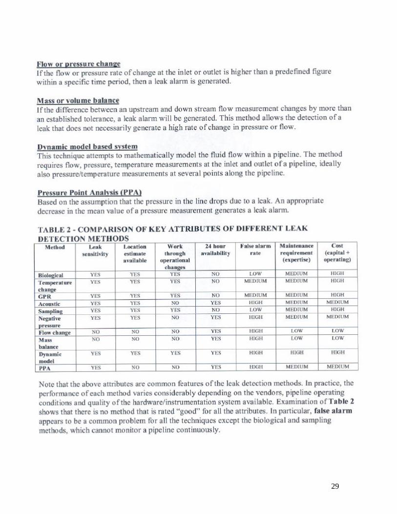
29

30

31

V References

Amir, N., and Shimony, U. “A Discrete Model for Tubular Acoustic Systems with Varying Cross Section, Part 1 Theory, Part 2 Experiments. Acustica Vol. 81 (1995) pp 450-474 Bassim, M.N., and Tangri, K.”Leak Detection in Gas Pipelines using Acoustic Emission”, Proceedings from International Conference on Pipeline Inspection, Edmonton Alberta, pp. 529-544, Canada, 1984. Blackstock, D. T., “ Fundamentals of Physical Acoustics”, Wiley 2000. Brodetsky, Igal and Savic, Michael, “Leak Monitoring Systems for Gas Pipelines” Proceedings: Institute of Electrical and Electronic Engineers, pp 111.17-111.20, New York, 1980. Brodetsky, Igal and Savic, Michael, “Digital Speech Processing, IEEE Int. Conf. On Acoustics, Speech and Signal processing, Apr 27-30 1993, Minneapolis MN. Campbell, M. and Greated, C., “ The Musicians Guide to Acoustics- Chapter 14”, Schirmer Books, pp. 525-547, New York, 1987. Cist, D.B., and Schutz, A.E. “State of the Art Pipe & Leak Detection, A Low Cost GPR Gas Pipe & Leak Detector, DE-FC26-01NT41317” U.S. Department of Energy Report, pp. 1-5, November 2001. Crouch, A. E., Burkhardt, G. L., “The Non-Linear Harmonic Method for Detection and Characterization of Mechanical Damage in Pipelines. Int. Chem. And Pet. Industry Inspec. Tech Topical Conf, Houston Texas June 1999. Crouch, A. E., “Optimizing the Nonlinear Harmonic Method for Detection of Mechanical Damage, Pipeline Pigging, Integrity Assessment and Repair, Houston Texas, Feb. 2000. DECI Newsletter, “Acoustic Emissions from Leaks”, http://www.deci.com/oct96.htm, Dunegan Engineering Consultants Inc., October 1996. Dunegan, H.L., “A New Acoustic Emissions Technique for Detecting and Locating Growing Cracks in Complex Structures”, Dunegan Engineering Consultants Inc. Report, pp. 1-9, May 2000. Ferdinand, M., “Building an Acoustic Emission Data Analysis Program”, Sensor Online Magazine http://www.sensormag.com, September 1999. Flournoy, N. E., and Schroeder, W.W., “Development of a Pipeline Leak Detector”, The Journal of Canadian Petroleum Technology, Vol. 17, No. 3, pp. 33-36, July 1978.

32

Gilmore R. E. “Lost Gas Speaking,” Gas Age-Record 1-4 ,July 6, 1935. Hall, D. E. “Musical Acoustics-Chapter 16 Sound Reproduction” , Wadsworth Publishing Company, pp. 374-388, Belmont CA, 1980. Hogan D.P., “ Field Results with Sonic Pinpointing”- Progress report 64-D-213, presented at the 1964 A.G.A. Operating Section distribution Conf. Huebler, J.E., “Leak Detection and Measurement Facts”, Gas Utility Manager Online Magazine, http://www.gasindustries.com, February 2000. Huebler, J.E., “Detection of Unauthorized Construction Equipment in Pipeline Right of Ways”, Presentation given at U. S. Department of Energy, National Energy Technology Center Natural Gas Infrastructure Reliability Industry Forums, Morgantown, WV, September 2002. Jette, N., Morris, M.S., Murphy J.C., and Parker, J.G.,”Active Acoustic Detection of Leaks in Underground Natural Gas Distribution Lines”, Materials Evaluation Journal, Vol. 35, Iss. 10, pp. 90-96, 99, October 1977. Jolly, W.D., Morrrow, T.B., O’Brien, F.F., Spence, H.F., and Svedeman, S.J., “New Methods for Rapid Leak Detection in Offshore Pipelines”, Final Report for U.S. Department of the Interior Minerals Management Service, pp. 1-84, April 1992. Kennedy, J.L., “Oil and Gas Pipeline Fundamentals” PennWell Books, Tulsa Oklahhoma, 1984. Kovecevich, J.J., Sanders, D.P., Nuspl, S.P., Robertson, M.O., “Recent Advances in Application of Acoustic Leak Detection to Process Recovery Boilers”, Babcock and Wilcox Report No. BR-1594, pp. 1-7, http://www.babcock.com, September 1995. Larson D.B. “Practical use of sound amplifiers in gas leak detection,” Proc. Pacific Coast Gas Association 30,81-82, 1939. Leis, B.N., Francini, R.B., Stulen, F.B., Hyatt, R.W., and Norman, R., “Real Time Monitoring to Detect Third Party Damage”, Proceedings of the Eigth International Offshore and Polar Engineering Conference, Montreal Canada, pp. 34-38, May 1998. Lee, M, and Lee J., “Acoustic Emissions Technique for Pipeline Leak Detection”, Key Engineering Vols. 183-187, pp. 887-892, Trans Tech Publications, Switzerland, 2000. McElwee L. A. and Scott T.W., “The Sonic Leak detector”, Am. Gas J. 184, 14-17, 1957. Moorthy, J. K., “Non destructive testing”, Proceedings of the 13th world conference on non destructive testing, Brazil, October 1992.

33

“Novel Devices Determines and Locates Gas Leaks by Sound”, Gas Age 124, 21-22, 1959. Parker, John, “Acoustic Detection and Location of Leaks in Underground Natural Gas Distribution Lines”, John Hopkins APL Technical Digest, V2, N2, Apr-Jun, pp. 90-101, 1981. Peterson, Arnold, Gross, Ervin., “Hand book of noise measurement” 1978. Proakis, J. G. and Manolakis, D.G., “ Digital Signal Processing, Prentice Hall, 1996 Qian, Shie,”Introduction to Time-Frequency and Wavelet Transforms, Prentice Hall, 2002 Raijtar, J.M., Muthieh, R., and Scott, L.R., “ Pipeline Leak Detection System for Oil Spills Prevention”, USDOE and New Mexico Waste-management Education and Research Consortium, Technical Completion Report, Project # WERC-01-4-23222, pp. 601-614, August 1994. Reid, J. M. , Hogan D.P. and Michel P. L., “ A New Approach to Pinpointing Gas Leaks with Sonics” DMC 61-22, presented at the 1961 A.G.A. Operating Section Distribution Conference. Richardson, R.B., Listening for leaks, Gas Age-Record, 47-48, July 30, 1935. Rocha, M. S., ”Acoustic Monitoring of Pipeline Leaks”Paper # 89-0333, ISA, 1989 Salava, T., “Acoustic Monitoring on Gas Pipelines by System AMOS” ETOS Advertisement, pp. 1-3, http://web.telecom.cz/etos/amosw.htm, 1999 Seaford, H.. “Acoustic Leak Detection through Advanced Signal Processing Technology”, ERA Technology Ltd. Surrey, England, May, 1994. Settles, G.S., “Imaging Gas Leaks using Schleiren Optics”, ASHRAE Journal, pp.19-26, July 1997. Shack, W.J., Ellingson, W. A., and Youngdahl, C.A., “Development of a Noninvasive Acoustic Leak Detection System for Large High Pressure Gas Valves”, ISA Transactions, Vol. 19, No. 4, pp. 65-71, 1980. Sharp, D.B. and Campbell, D.M., “Leak Detection in Pipes Using Acoustic Pulse Reflectometry”, EPSRC Report, pp. 1-14, http://www.acoustics.open.ac.uk, 1996.

34

Shimony, A.U. and Rosenhouse, G., “A Discrete Model for Tubular Acoustic Systems with Varying Cross Section- The Direct and Inverse Problems, Part 1 and Part 2: Theory and Experimants”, Acustica Journal, Vol. 81, pp. 450-474, 1995. Shinha, N.D., “Multi-Purpose Acoustic Sensor”, Los Alamos National Lab., Presented at the National Gas Infrastructure Reliability Industry Forum, Sept. 16-17, 02 at NETL, Morgantown WV. Varma, V.K., “Gas Pipeline Safety: ORNL’s Role” ORNL Review Vol. 35, No. 2, pp. 1-3, http://www.ornl.gov, 2002. Smith, O. L.”The soundograph system for gas leak detection,” Gas Age-record 381-383(Apr 15, 1933) Taghavie, R.R. @ all, “Noise from Shock Containing Jets of Non-Uniform Geometry”, Int. J. of Aeroacoustics, ISSN 1475 472x. Vol 1, No 1, March 2002 Thompson, W.C. and Skogman, K.D., “Application of Real Time Flow Modeling to Pipeline Leak Detection”, J. of Energy Resources Tech., transactions of ASME, v 105, n 4, p536-541, Dec,. 1983. Varma, V.K., “State of the Art Natural Gas Pipe Inspection” U. S. Department of Energy Report, National Energy Technology Center, pp. 1-5, 2002, Sept 16-17, Natural Gas Infrastructure Reliability Industry Forum, NETL, Morgantown WV. Watanabe, K., Matukawa, S., Yukawa, H., and Himmelblau, D. M., “Detection and Location of a Leak in a Gas Transport Pipeline By a New Acoustic Method”, Hosei University, Department of Instrumentation and Engineering Journal, N1, pp. 129-157, March 1985. Watanabe, K., and Himmelblau, D. M., “Detection and Location of a Leak in a Gas Transport Pipeline By a New Acoustic Method”, AIChE Journal, V 32, N10, pp. 1690-1701, 1986. Watanabe, K., Koyama, H., and Ohno, H., “Location of Leaks in a Gas Transport Pipeline By Acoustic Method”, Instrument Society of America Technical Paper, No. 87-1106, pp. 619-626, 1987. Wylie, E. B., and Streeter, V. L. with Suo, L., “Fluid Transients in Systems” Prentice Hall, 1993. Zhang, Jun,”Designing a Cost Effective and Reliable Pipeline Leak Detection System”, Pipeline Reliability Conference, Houston, USA, November 19-22, 1996.