Technology Adoption and Productivity Growth:Evidence from Industrialization in France *

Réka Juhász Mara P. Squicciarini Nico Voigtländer(Columbia, NBER, and CEPR) (Bocconi and CEPR) (UCLA, NBER, and CEPR)

This version: 14 October, 2020

Abstract

We construct a novel plant-level dataset to examine the process of technology adoption duringa period of rapid technological change: The diffusion of mechanized cotton spinning during theIndustrial Revolution in France. We document new stylized facts that can help explain why majortechnological breakthroughs tend to be adopted slowly and – even after being adopted – take timeto be reflected in aggregate productivity statistics. Before mechanization, cotton spinning wasperformed in households, while production in plants only emerged with the new technology around1800. This allows us to isolate the plant productivity distribution of new technology adopters inmechanized cotton spinning. We find that this distribution was initially highly dispersed. Overthe subsequent decades, mechanized spinning experienced dramatic productivity growth that wasalmost entirely driven by a disappearance of plants in the lower tail. In contrast, innovations inother sectors (with gradual technological progress) shifted the whole productivity distribution. Wedocument rich historical and empirical evidence suggesting that the pattern in cotton spinning wasdriven by the need to re-organize production under the new technology. This process of ‘trial anderror’ led to widely dispersed initial productivity draws, low initial average productivity, and – inthe subsequent decades – to high productivity growth as new entrants adopted improved methodsof operating the mechanized technology.

JEL: F63, O14

Keywords: Industrialization, Technology Adoption, Firm Productivity

*We thank Sandy Black, Bruno Caprettini, Diego Comin, Tarek Hassan, Michael Huberman, Felix Iglhaut, MarkusLampe, Nils Lehr, Bob Margo, Joel Mokyr, Tomasso Porzio, Diego Puga, Eric Verhoogen and numerous seminar audi-ences at Bocconi, Boston University, Cologne, Columbia, Leuven, Lund, Montreal University, Namur University, PennState, Yale, UCL, UCLA, and participants at the 2020 NBER Summer Institute Meetings, the 2019 SED meetings, the1st Workshop of Economic History in Bologna, “The Transnational History of French Industrialisation Before 1914”conference, and the IGC-Stanford conference on Firms, Development and Trade 2019 for helpful comments and sug-gestions. We thank Gaia Dossi, Johanna Gautier, Angelo Krüger, Lorine Labrue, Simon Margolin, Marie Michaille,Alberto Mola, and Sebastian Ottinger for excellent assistance throughout the construction of the dataset, GuillaumeDaudin for kindly sharing data, and Eugene White for sharing his expertise of hyperinflation during the French Revo-lution. Financial support from the National Science Foundation (Grant # 1628866) is gratefully acknowledged.

[T]here were strong pairwise complementary relations between factory organization and ma-chinery [...] employers needed to simultaneously determine the choice of technique, the levelof worker effort, and the way incentives were set up and communications and decisions flowedthrough the firm hierarchy. [...] Factories were the repositories of useful knowledge ... but theywere also the places in which experimentation took place. – Mokyr (2010, pp. 345-46)

1 Introduction

The diffusion of innovation is at the core of aggregate productivity growth in the long run. Despiteits importance for economic development, understanding the determinants and effects of tech-nology adoption has proven difficult. As a consequence, the literature faces a number of openquestions. For example, many technologies that ended up being widely adopted – such as hybridcorn seed in agriculture (Griliches, 1957) or by-product coke ovens in the iron and steel industry(Mansfield, 1961) – were slow to diffuse across firms.1 This slow adoption is particularly puz-zling given that new technology can provide a substantial boost to firm productivity (Syverson,2011; Bloom, Eifert, Mahajan, McKenzie, and Roberts, 2013; Giorcelli, 2019). There is also asecond, well-documented puzzle: When major innovations such as information technology (IT) orelectricity spread across firms, the widely expected boost in aggregate productivity proved hard todocument in the data. This prompted Robert Solow to remark in 1987 that “[...] what everyonefeels to have been a technological revolution, a drastic change in our productive lives, has beenaccompanied everywhere, including Japan, by a slowing-down of productivity growth, not by astep up. You can see the computer age everywhere but in the productivity statistics.”2

A natural lens to study aggregate effects of technology adoption is the firm (or plant) produc-tivity distribution – an approach that has gained prominence over the last two decades (c.f. Melitz,2003; Hsieh and Klenow, 2009; Combes, Duranton, Gobillon, Puga, and Roux, 2012; Perla andTonetti, 2014). However, applying this framework to technology adoption is difficult for numerousreasons: The specific technology used by firms is rarely directly observed, and even if it is known,new and old technologies typically coexist within narrowly defined sectors, or even within plants.In addition, the productivity distributions under the old and new technologies are not independent– a plant’s productivity with the old technology can affect its propensity to adopt innovations.These factors render it difficult to isolate aggregate productivity growth among adopters of thenew technology. One approach to tackle these challenges is the use of randomized control trials(RCTs), which provide clean identification of the effects of technology at the firm level (Bloomet al., 2013; Atkin, Chaudhry, Chaudry, Khandelwal, and Verhoogen, 2017; Hardy and McCasland,

1The more general observation that technology is often slow to diffuse is attributed to Rosenberg (1976). See Halland Khan (2003) and Hall (2004) for surveys of the literature on technology diffusion. Comin and Hobijn (2010)document substantial lags in the adoption of new technologies, estimating that the variation in adoption lags acrosscountries can account for at least one-quarter of per capita income disparities.

2New York Times, July 12, 1987, p. 36. Such productivity puzzles are not restricted to the introduction of com-puters: David (1990) documents similar trends following the diffusion of electricity earlier in the 20th century.

1

2016). However, the relatively small sample size and short time horizon do not allow for a system-atic analysis of the firm productivity distribution.

This paper bypasses the typical limitations by exploiting a unique historical setting – the adop-tion of mechanized cotton spinning in France during the First Industrial Revolution. Mechanizedcotton spinning had been invented in Britain and – if operated efficiently – promised huge pro-ductivity improvements. We hand-collect novel plant-level data from historical surveys coveringmechanized cotton spinning and two comparison sectors – metallurgy and paper milling – at twopoints in time, around 1800 and in 1840. Importantly, in 1800, mechanized cotton spinning hadonly recently been adopted in France. Four decades later, the technology had reached maturity(Pollard, 1965). Thus, the time period that we study encompasses both the initial phase of adop-tion and the period when the new technology had widely spread.

Our empirical strategy relies on a number of features of the historical setting. First, beforethe emergence of the new technology, cotton spinning was performed in home production withhand-operated spinning wheels (see the illustration in Appendix Figure A.1). Plants – or let alonefactories – did not exist in cotton spinning prior to its mechanization. The new technology – thefamous spinning jenny and the subsequent spinning mule – required the organization of produc-tion in cotton mills (see Appendix Figure A.2). Thus, all cotton spinning facilities in our datasetoperated mechanized spinning in a central location, that is, in a plant.3 This allows us to isolatethe productivity distribution specific to the new technology and to examine its evolution over time.Second, the mechanized spinning technology changed relatively little between 1800 and 1840. Wecan thus narrow down potential drivers of productivity differences across plants and over time:With the underlying technology being very similar, productivity differences likely resulted fromthe more or less efficient operation of the new technology.4 This goes beyond existing work,where productivity changes due to technology adoption reflect both the productivity differentialof the new technology itself and the efficiency with which this technology is operated. Third, wedocument that owners who set up mechanized cotton spinning plants typically had a backgroundin banking and finance as opposed to handspinning, suggesting that productivity under the newand old technologies were not systematically related.

3Throughout the paper, we refer to mechanized cotton spinning production organized in a central location as aplant. This is in order to delineate the organization of mechanized production from earlier organizational forms. Inparticular, under the pre-industrial putting-out system across much of France, local merchant-manufacturers organizedhome production across a multitude of households. They typically owned the capital equipment (the spinning wheels),which they gave to spinners together with the raw material, then collecting the spun yarn and marketing it (Huberman,1996). This system was akin to ‘firms’ employing many external workers who performed production in scatteredlocations, typically for a piece-rate as opposed to a wage. Our survey of cotton spinning in 1806 allows us to eliminatethe few cases of home production that were recorded by the enumerators. We thus focus on producers that organizedmechanized production in plants.

4We do not claim that there was no technological progress in mechanized cotton spinning whatsoever. The tech-nology did experience incremental changes. We show, using a number of robustness checks across plants and overtime, that these do not explain our results.

2

We document three main findings for mechanized cotton spinning plants: 1) we observe ahighly dispersed productivity distribution in the initial period (1806) relative to 1840; 2) we esti-mate that the mechanized cotton spinning industry underwent a substantial (82%) increase in plantproductivity between 1806 and 1840 after mechanization had already been adopted; 3) this aggre-gate productivity growth in mechanized cotton spinning had a strong lower-tail bias: It was largelydriven by the disappearance of lower-tail plants.

We compare the evolution of the plant productivity distribution in cotton spinning with twocomparison sectors – metallurgy and paper milling. Importantly, in these sectors, production wasalready organized in plants before the Industrial Revolution because of their reliance on waterpower and high-fixed-cost machinery (see the illustrations in Figures A.4 – A.7 in the appendix).Thus, operational and organizational knowledge had already diffused. Technological progress inthese sectors was more gradual and took the form of integrating new capital vintages into existingproduction setups – as opposed to the radical shift from home-based to factory-based productionin cotton spinning. We find that the whole productivity distribution shifted to the right in thecomparison sectors.

To rationalize these findings, we build on a mechanism that has been emphasized by historiansand back it with new empirical evidence: Adopting mechanized cotton spinning required plants tolearn best-practice methods along multiple dimensions. This is consistent with a setting in whichplants learn about the optimal use of multiple inputs or tasks that in turn exhibit complementaritiesin the production function. We show that these features initially (when plants have little experiencein the optimal performance of tasks) lead to a fat lower tail in the plant productivity distribution.Over time, as plants learn about the efficient use of multiple inputs (tasks), the lower tail disappears.We provide rich historical evidence consistent with this mechanism. Mechanization required themove to factory-based production, which represented an important organizational challenge: Howshould the layout of the mill be designed? How should machines be powered and how should thework flow be organized? How should workers – not used to the hierarchy and discipline of factoryproduction – be recruited and managed? These organizational innovations proceeded via a processof trial and error, and the diffusion of organizational knowledge took time. As Allen (2009, p.184)writes: “The cotton mill, in other words, had to be invented as well as the spinning machinery per

se.”We provide several pieces of evidence in line with the proposed mechanism. First, we show

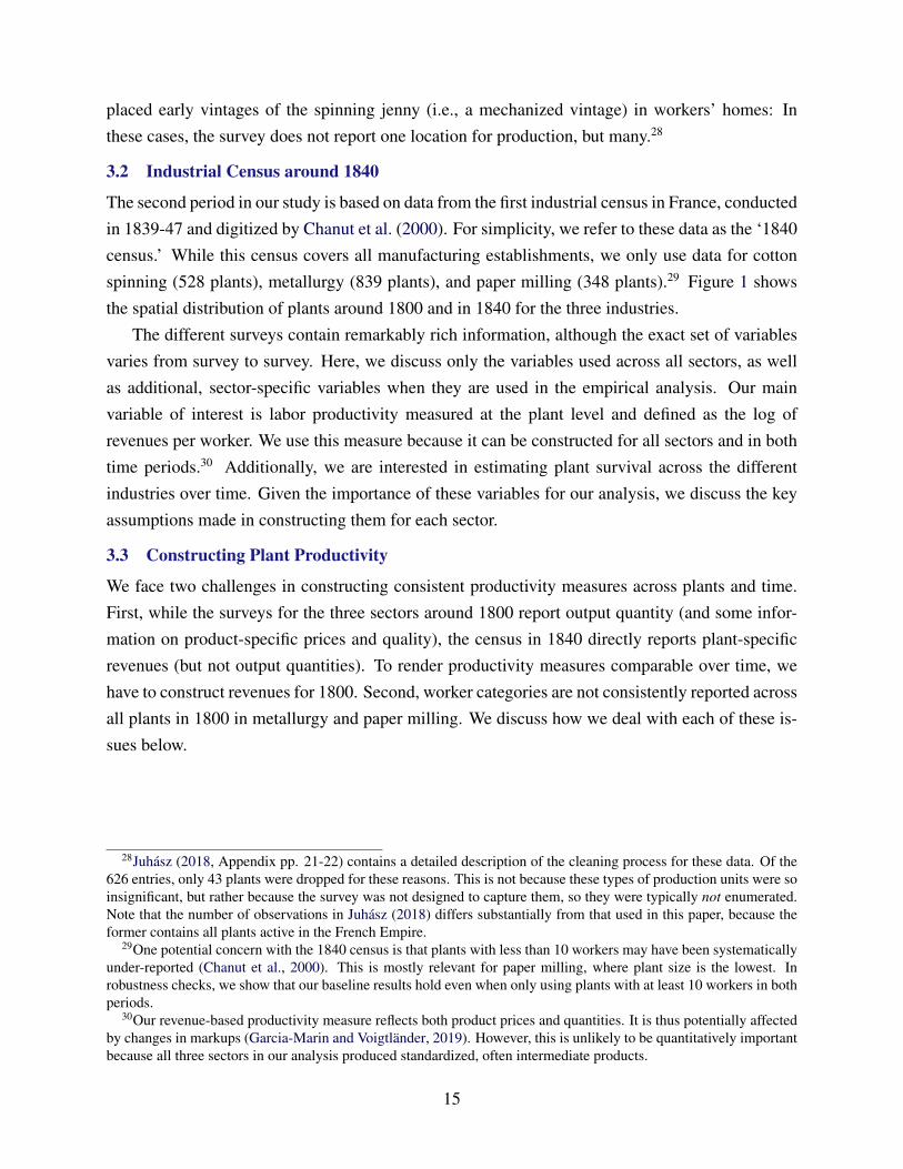
that the exit rate of plants in mechanized cotton spinning was substantially higher than in othersectors between 1800 and 1840. This is consistent with the idea that early adopters faced consid-erable uncertainty about best-practice methods in production. Coherently, we show that exitingplants were substantially less productive than those that survived. Second, using plant age, weshow that cotton spinning plants that entered the market later had higher productivity. This finding

3

supports our argument that knowledge about the optimal organization of mechanized cotton spin-ning diffused slowly over time. Moreover, the productivity advantage of younger plants is only arobust feature in cotton spinning around 1800. Younger spinning plants were not more productivein 1840; and in metallurgy, young plants were as productive as older ones in both periods.5 Thisis consistent with the idea that later entrants in mechanized cotton spinning could draw from abetter pool of organizational knowledge, which evolved over time and reached maturity around1840. This process was muted in metallurgy, where plant-based production methods had been es-tablished much earlier. Finally, we examine our data for patterns compatible with learning effects.We find evidence supporting the spatial diffusion of knowledge: Plants located closer to otherhigh-productivity plants were themselves more productive, and this relationship is strong only forcotton spinning plants and only during the initial period of technology adoption. We show, using arich set of controls and placebo tests, that these results are unlikely to be driven either by selectioninto productive locations or by omitted variables.

Overall, our findings allow us to shed light on the two puzzles of slow adoption of major in-novations and slow aggregate productivity growth. In combination with rich historical evidence,the highly dispersed initial productivity distribution points to information disparities across cottonplants: The organization of factory production evolved via a process of trial and error such thatonly the most productive adopters, those that ‘stumbled’ onto the efficient organization of factoryproduction, survived. By 1840, information about the efficient organization of cotton mills haddispersed, leading to a much narrower distribution of plant productivity. Uncertainty about theoptimal organization of production with a new technology can thus explain why aggregate pro-ductivity gains for technologies are initially small. Early adopters need to experiment with theefficient organization of production, and most of them will inadvertently operate the new technol-ogy inefficiently. Consequently, the potential benefits of the new technology materialize relativelyslowly for the average plant. Our findings thus lend support to the view in the literature that theeffects of major new technologies, such as electricity and IT, appear slowly in industry productivity“due to the need to re-organize the operation of the entire manufacturing facility to make effectiveuse of this innovation” (Hall and Khan, 2003, p.8).

At the same time, potential adopters of a new technology expect that the knowledge about itsoptimal operation will improve over time. This creates incentives to delay entry. Indeed, we ob-serve that later entrants in cotton spinning had significantly higher productivity than early adopters.These findings can help to explain the slow diffusion of major innovations, especially if they re-quire a re-organization of production.

Our paper is closely related to a large literature on technology adoption. The most developedstrand of this literature explains the low rates of technology adoption in agriculture in developing

5Due to data limitations, we cannot conduct this exercise for paper milling.

4

countries.6 Given its importance in driving long-run sustained growth, understanding technologyadoption in manufacturing is arguably equally important. However, this strand of the literature ismuch smaller, perhaps due to the difficulty of observing and categorizing the use of diverse tech-nologies in manufacturing. The majority of recent papers circumvent this issue by using RCTsto understand the determinants of technology adoption (c.f. Bloom et al., 2013; Hardy and Mc-Casland, 2016).7 In line with our results, some of the evidence from experimental settings pointsto the importance of organizational barriers (Atkin et al., 2017). We contribute to this literature bystudying the full plant productivity distribution for one of the most famous innovations in history,both at the initial phase of technology adoption and once the industry had reached maturity. In-terestingly, our results suggest that the complex nature of production processes in manufacturingrelative to agriculture may be important. In cases where technology adoption requires a substan-tial re-organization of production, adoption may be slow and productivity effects may take time tomaterialize.

Second, theoretical and empirical research has pointed to the importance of firm dynamicsfor understanding aggregate productivity (Jovanovic, 1982; Melitz, 2003; Syverson, 2011). Akey insight of this literature is that – as there are large differences in productivity even withinnarrowly defined sectors – examining the entire distribution is critical for understanding aggregateproductivity (Hsieh and Klenow, 2009). We apply this insight to the arguably most importantstructural break in economic history: The First Industrial Revolution, which saw unprecedentedgrowth in manufacturing productivity (Crafts, 1985; Crafts and Harley, 1992; Galor, 2011). Sofar, productivity growth during this period has been studied mostly at the country level, or – insome cases – at the aggregate sectoral level. To the best of our knowledge, our paper is the firstto study the contribution of plant dynamics to manufacturing productivity improvements duringthe Industrial Revolution.8 In addition, we examine the puzzle of the slow diffusion of majortechnological innovations through the lens of the firm-productivity literature: Our findings suggestthat focusing on the entire distribution of plant productivity can help deepen our understanding of

6See for example Foster and Rosenzweig (1995), Munshi (2004), Bandiera and Rasul (2006), Conley and Udry(2010), Duflo, Kremer, and Robinson (2011), Suri (2011), Hanna, Sendhil, and Schwartzstein (2014), BenYishay andMobarak (2018), Beaman, Magruder, and Robinson (2014), and Emerick, de Janvry, Sadoulet, and Dar. (2016).

7One notable exception is Giorcelli (2019), who exploits a historical natural experiment to identify the productivityeffects of adopting modern management practices and modern machinery by Italian firms after WWII.

8Similar to our setup, but in the modern context, Collard-Wexler and De Loecker (2015) examine how a specificsector was affected by a major innovation: the introduction of the minimill in the steel industry starting in the 1960s.This led to large aggregate productivity increases via both technology upgrading of surviving producers and exit ofold incumbents. In contrast, our setting isolates productivity gains within the new technology, by separating it frompre-industrial home spinning. In other words, upgrading of existing ‘old’ producers is not present in our data, so thatexit, entry, and improvements all occur among operators of the new, mechanized cotton spinning technology. A relatedpaper in the historical context is Braguinsky, Ohyama, Okazaki, and Syverson (2015), who study the Japanese cottonspinning industry in the late 19th century and early 20th century. Rather than technology adoption, this paper focuseson the effects of acquisitions on acquired plants. These see a rise in productivity due to lower inventories and highercapacity utilization – which is likely a result of improved demand management.

5

technology adoption. This is in line with Foster, Grim, Haltiwanger, and Wolf (2018), who provideempirical support for the argument by Gort and Klepper (1982) that periods of rapid innovationare associated with a surge in firm entry, followed by a period where experience with the newtechnology is accumulated, eventually leading to a shakeout where unsuccessful firms (or plants)exit.9

Third, our paper is related to a strand of the literature that studies the role of organizationalchanges during the Industrial Revolution. In a set of papers Sokoloff (1984, 1986) shows thatin the first half of the 19th century in the United States, both mechanizing and non-mechanizingindustries displayed i) marked increases in firm scale as measured by the number of employees,and ii) substantial increases in productivity. Sokoloff speculates that these results are consistentwith two important sources of productivity growth during the early stages of industrialization: di-vision of labor and modifications in routines. However, a crucial distinction between the US andFrench context is that the former did not have an important cotton handspinning sector prior tomechanization. Thus, mechanized cotton spinning firms not only had to introduce the new tech-nology to the US, but they also had to create the necessary infrastructure to supply raw materialsand to market their final products (Ware, 1931).10 In the European context, the seminal work byPollard (1965) documents important organizational innovations (in what we would call ‘manage-ment’ today) that took place in the first half of the 19th century in Britain.11 We contribute to thisliterature in the following ways. First, we show that, similar to the US, plant size and industryproductivity were growing in France across a variety of sectors. This suggests that these patternsare a general feature of the early process of industrialization. Second, our main interest lies inunderstanding productivity growth during the process of technology adoption. While our resultsare consistent with Sokoloff’s conjecture that changes in firm organization contributed to rapidproductivity growth during this period, our findings highlight that these productivity gains tooktime to materialize. Third, our unique setting allows us to isolate the effect of technology adop-tion from other factors such as the development of input or output markets. Finally, we analyze

9The literature has typically measured innovation via firm-level R&D expenditures or patents. Since these maymiss important dimensions of firm activity (such as learning), Foster et al. (2018) rely on broader indicators for thepresence of innovation: firm entry and productivity growth. Due to the indirect nature of these indicators, Foster et al.(2018) are reluctant to conclusively tie their results to technological innovation. Our unique setting has the advantagethat we can isolate all plants in the cotton industry that operated a major new technology and track their productivitydistribution over time.

10This type of confounder is not present in the French setting, which had a long history of handspinning beforethe Industrial Revolution. Raw cotton and cotton yarn markets were well-developed across France by 1800. Thus,one cannot replicate our results in the US context, despite the availability of US firm level data across a broader setof industries. In addition, the first US manufacturing census with wide coverage is from 1820. At this point, the USmechanized sector was arguably more mature than the French one from 1806. In other words, the early first cottonindustry survey in France allows a unique look at its infancy period.

11Subsequent research in this area is discussed in Mokyr (2010). Squicciarini and Voigtländer (2015) show thatupper-tail human capital played an important role in the industrialization of France.

6

the overall plant productivity distribution and are thus able to shed new light on how productivitygrowth evolved.

The paper is structured as follows. The next section discusses the historical context. Section3 describes the construction of our novel dataset from archival sources, while Section 4 presentsand discusses our empirical results. Section 5 draws conclusions from our results for technologyadoption during periods of major innovation.

2 Historical Background

Early nineteenth century France presents an ideal setting for our study of technology adoption.While England was the first country to industrialize, France was a close follower and structurallysimilar to England (Crafts, 1977; Voigtländer and Voth, 2006). The flagship inventions of theIndustrial Revolution – most notably the spinning jenny – were developed in Britain. Franceadopted these widely during the first half of the 19th century and witnessed a similar accelerationin industrial output as Britain (Rostow, 1975).12 By focusing on France, we thus study the effectsof technology adoption in the context of an industrializing economy that was (at least initially)mostly adopting technology developed elsewhere.

Our empirical analysis builds on three pillars that emerge from the historical context. First, thenew cotton spinning technology entailed a move from home-based to factory-based production.This allows us to isolate the productivity distribution of adopters of the new technology. Second,we compare the productivity distribution in cotton spinning to two other sectors: metallurgy andpaper milling. Production in these sectors was already organized in plants prior to the IndustrialRevolution and experienced mostly incremental technological change that did not entail a drasticreorganization of the production process. Using these comparison sectors helps us to distinguishthe effect of adopting a major new technology in cotton spinning from other trends that may haveaffected productivity distributions more broadly. Third, we discuss the historical evidence for themechanism that arguably explains our empirical findings: The move to large-scale factory-basedproduction in cotton spinning required the development of best-practice methods for organizingproduction through a process of trial and error.

2.1 Mechanized Cotton Spinning

Development of Mechanized Spinning in Britain. Cotton textiles was the flagship industry of theFirst Industrial Revolution, contributing one-quarter of TFP growth in Britain during the period1780-1860 (Crafts, 1985). Cotton spinning is the process by which raw cotton fiber is twistedinto yarn. Traditionally, this task was performed mostly by women in their homes, using a simplespinning wheel (see Figure A.1 in the appendix). With this old technology, each spinner was ableto spin only one thread of yarn. The industry was rurally organized and generally centered around a

12Appendix A.1 provides a more detailed discussion of the Industrial Revolution in France.

7

local merchant-manufacturer who would supply spinners with the raw cotton, collect their output,take care of the marketing, and often also owned the spinning wheels (Huberman, 1996).

The breakthrough “macro-invention” in spinning was forged in Britain in 1765, when JamesHargreaves invented the spinning jenny. This made it possible to spin multiple threads simulta-neously, as twist was imparted to the fibre not by using the worker’s hands, but rather by usingspindles. In 1779, Samuel Crompton further improved the design, inventing the water-poweredspinning mule (see the left panel in Figure A.2). The productivity effect of these innovations wasenormous. Allen (2009) estimates that the first vintage of the spinning jenny alone led to a three-fold improvement in labor productivity. Correspondingly, the price of yarn declined rapidly inthe late 18th century (Appendix Figure A.3), especially for the highest-quality yarn, where pricesdeclined from 1,091 pence per pound to 76 pence per pound in real terms between 1785 and 1800(Harley, 1998).13

The mechanization of cotton spinning required production to be organized within factories fortwo reasons. First, the dependence on high fixed-cost inanimate power sources (such as water andsteam) led to the concentration of production in one location.14 Second, mechanized productionincreased the need for monitoring workers, who were now paid factory wages rather than for theirhome-produced output (Williamson, 1980; Szostak, 1989).15 As production moved to factories(see the illustration in the right panel of Figure A.2), cotton spinners faced a set of new challengesin organizing production effectively. We return to this issue in the next section.

Adoption of Mechanized Spinning in France. Mechanized spinning was adopted with some lag inFrance. Efforts to adopt the technology had begun with state support during the Ancien Régime. Bythe beginning of our sample period in 1806, the large-scale expansion of the industry documentedin Juhász (2018) had just begun: The technology was known throughout the country (Horn, 2006),and a number of domestic spinning machine makers had been established (Chassagne, 1991). Thespinning machinery itself was produced mainly in France (using British blueprints) because of a

13Harley (1998) collected price data for three different qualities of yarn from British sources: 18, 40 and 100 countyarn (the count is an industry-wide standard that refers to the length per unit mass, implying that higher counts arefiner). While all counts saw striking price declines (see Figure A.3), this trend was most pronounced for the finest,highest-quality varieties. Machine spinning had the largest impact on the fine high-quality yarn, which British hand-spinners had not been able to effectively produce and to which the mule-jenny (a subsequent vintage of the machineintroduced in the late 18th century) was well-suited (Riello, 2013). Our data include information on the type of yarnproduced, allowing us to account for quality differences across plants.

14The initial spinning jenny was hand-powered, but newer vintages of machinery that used inanimate sources ofpower (the throstle and the mule) were rapidly developed.

15Huberman (1996, p. 11) describes the need for monitoring in mechanized cotton spinning: “If there were multiplebreakages of yarn on the larger machines, the mule had to come to a complete stop to piece the broken threads. Therewas also doffing, when the reels were full of spun cotton, the mule had to be stopped and the reels removed. Finally,there was cleaning. At all times, the spinners could expend effort as they were motivated to, and without propersupervision or incentives they could disguise how hard they could in fact work.” This created a strong need formonitoring, so that even early hand-powered machines (a particular vintage of spinning machinery) were housed inthe “garrets of cottages and later in sheds” (Huberman, 1996, p. 11).

8

ban on exporting machinery from Britain until 1843 (Saxonhouse and Wright, 2004).A number of features in the historical setting allow us to study how technology adoption af-

fected productivity growth. First, mechanized spinning technology operated in centralized loca-tions (plants), while the old technology relied on home production. This allows us to identify allproducers that used the new technology, i.e., all plants observed in our data.16 Consequently, weare able to isolate the productivity distribution for plants that used the new, mechanized technology.

Second, the sharp break in organizational requirements under the new technology rendered ex-perience with the old technology effectively useless: The type of skills necessary for successfullyrunning mechanized cotton spinning factories were very different from those required under the oldcottage-industry technology. Correspondingly, historical evidence suggests that most owners whooperated the new technology in France around 1800 did not have a background in the old technol-ogy. Table 1 presents information on the socio-economic background of the owners of mechanizedcotton spinning establishments for the early period of technology adoption (1785-1815). Basedon these figures, the vast majority of owners were “traders, bankers and commercial employees”(62.5%), while only a small faction (10.2%) came from the production side, i.e. “workers and me-chanics,” and three-quarters of this latter group were in fact highly skilled mechanics Chassagne(1991, p. 274).17

Third, during our sample period, the vintages of capital in cotton spinning and the technologyremained largely unchanged.18 This renders it unlikely that our analysis is confounded by theintroduction of novel technology after the onset of mechanized spinning.19 We can confirm thisin our data, because the plant survey in 1806 asked which vintage of capital plants used. We findthat both the throstle and the mule-jenny were widely used by existing cotton mills in France. Thenext vintage to appear (the self-acting mule – a fully automated machine) did not spread until the1840s, i.e., after our sample period ended (Huberman, 1996). Moreover, in contrast to Britain,mechanized cotton spinners in France did not switch from water to steam power to a large extent,

16We follow Mokyr (2010, p. 339) in defining factory-based production as “the precise circumscription of workin time and space, and its physical separation from homes.” This definition is solely based on the organization ofproduction; it does not rely on the use of inanimate sources of power. This is important because it allows us to refer to‘factory’ or ‘plant’ production even when our data do not include specific information on power sources. Section 3.1describes how we clean the data of a small number of observations that mix features of home and factory production.

17It is possible that some merchant-manufacturers previously involved with handspinning are reported under thecategory “traders, bankers and commercial employees.” However, Chassagne (1991, p. 274) clarifies that “Two-thirdsof entrepreneurs came from a general trade background, predominantly in fabric and cloth, which proves the predom-inance of commercial factors in the launching and success of industrial enterprises.” This highlights the importance ofmarketing skills (as opposed to previous experience with handspinning) in setting up cotton spinning factories.

18There were three main types of machinery in use: the spinning jenny, the throstle and the mule-jenny. These werenot good substitutes; in particular, the mule-jenny was well-suited to spinning higher-count, finer yarns (Riello, 2013).

19This is not to say that there were no improvements of the existing technology, or that plants did not increasetheir capital intensity. In robustness checks, we show that our main results are unlikely to be driven by these types ofincremental improvements to the technology.

9

owing to the fact that France was not particularly well-endowed with coal (Cameron, 1985).20

Fourth, the historical literature summarized in Juhász (2018) underlines that the French neededto figure out many aspects of operating the technology efficiently themselves. That was partlybecause of the ban on machine exports and emigration of engineers and skilled workers fromBritain throughout our sample period (Saxonhouse and Wright, 2004), and partly because a lot ofthe learning that needed to be done was tacit (Mokyr, 2001, 2010).21

2.2 Comparison Sectors: Metallurgy and Paper Milling

We compare the evolution of the plant productivity distribution in mechanized cotton spinning totwo other sectors: metallurgy and paper milling. The key feature of both comparison sectors isthat they had already organized production in plants since well before the Industrial Revolution.In metallurgy, plant production was mostly due to the reliance on high fixed-cost machinery suchas the furnaces used both in smelting and refining. In paper milling, production was organized inplants because of the beating engine’s reliance on water-power.22

Technological change in the two comparison sectors was introduced gradually and within theexisting organization of production. The switch from charcoal to coal in metallurgy could beintroduced by modifying a plant’s existing machines and ovens (see the illustration in FiguresA.4 and A.5 in the appendix). In paper milling, the mechanization of forming paper (one stepin the production process) did not substantially alter the layout of the factory or other parts ofthe production process (see Figures A.6 and A.7). Moreover, the adoption of new technologiesin both sectors was slow in France. Adoption began in the 1820s, and it was fairly modest until1840. In metallurgy, the switch to coal was delayed because – in contrast to Britain – the relativelylow price of charcoal kept the old (charcoal-based) technique profitable until the new (coal-based)technology’s efficiency had risen (Allen, 2009). The new production processes using coal – cokesmelting and the puddling process in refining – were both introduced around the 1820s in Franceand gradually adopted thereafter. By 1827, there were only four French departments where ironwas smelted with coke. The adoption of the puddling process was more widespread, with 149puddling furnaces in use across 15 out of 86 departments (Pounds and Parker, 1957).23

20This is confirmed in our data for 1840, showing that the majority of cotton spinning plants were still using waterpower (see Table D.3 in the appendix).

21Some British involvement in technology transfer took place despite the legal bans and the wars that occurredduring this time period (Horn, 2006; Chassagne, 1991). However, while foreign technology transfer likely playedsome role in French learning, machines had to be produced domestically, workers were local, and some fundamentalfactors were different (such as the relative scarcity of coal).

22The beating engine breaks down the raw input vegetable matter into cellulose fiber. The production process isdescribed in more detail in Appendix A.3.

23We can also verify indirectly that the new coal-based technology was introduced slowly in metallurgy: Adoptingcoal required a switch from water to steam as power source (Pounds and Parker, 1957), and the latter is reported byplants in 1840. Only 16% of plants in metallurgy report using steam-power, suggesting that the vast majority of themstill used the older charcoal-based technology (see Table D.3 in the appendix).

10

In paper milling, the adoption of mechanized paper formation was similarly slow. While evi-dence on the adoption of mechanized paper-making is relatively scarce, our plant-level data from1840 suggest that the technology had not been widely adopted. Only 10 (out of 348) plants explic-itly mention having mechanized their production process, and only 42 plants report using steampower, which was necessary for the mechanized machine.

Given these features, the plant productivity distributions in metallurgy and paper milling re-flect the same mix of old and new technology vintages that is typically observed in standard datasources. Observing two industries that were already organized in plants prior to the IndustrialRevolution allows us to disentangle the productivity dynamics that were specific to mechanizedcotton spinning from broader trends that affected the productivity distributions of all industriessimultaneously.

2.3 The Challenging Transition to Factory-Based Production in Cotton Spinning

The transition to large-scale factory-based production has been characterized as “one of the mostdramatic sea changes in economic history” (Mokyr, 2010, p. 339). While cotton spinning was notthe first sector to organize production in factories, the organizational changes during its industrial-ization went far beyond the experience made by other sectors. By the time cotton spinning millsreached maturity around 1830 in Britain (Pollard, 1965), they were larger, with a finer division oflabor and a greater concentration of capital than production units in other sectors that had beenorganized as plants earlier (Chapman, 1974). However, the biggest change was the developmentof flow production – the production of standardized goods in huge quantities at low unit costs by“arranging machines and equipment in line sequence to process goods continuously through a se-quence of specialized operations” (Chapman, 1974, p. 470). It is this synchronisation of highlyspecialized machines that distinguishes the cotton spinning factory as a “fully-evolved factory”from earlier developments (Chapman, 1974, p. 471).

Developing efficient cotton spinning mills meant solving organizational challenges along mul-tiple dimensions. As Allen (2009, p.184) writes:

“The spinning jenny, water frame and mule were key inventions in the mechanization of cottonspinning, but they were only part of the story. [...] the machines had to be spatially organized,the flows of materials coordinated, and the generation and distribution of power sorted out.A corresponding division of labour was needed. The cotton mill, in other words, had to beinvented as well as the spinning machinery per se.”

Successful mill designs were observed and copied. Chapman (1970, p. 239) shows that early millsin England had a remarkably similar structure because plants quite literally copied the originaldesign of the Arkwright mills over and over again. Moreover, since few millwrights were qualifiedto build the power units of their mills, these were typically built by the same handful of engineers,qualified from experience (Chapman, 1970, pp. 239-40). It took time for design defects to be

11

improved; for example, contemporaries were aware of ventilation problems in the Arkwright-stylemills, but continued to use the same layout regardless (Fitton and Wadsworth, 1958, p. 98).

Beyond organizing the production process efficiently, the factory setting and the use of inan-imate power itself produced a host of new, unanticipated challenges. For example, fire hazardswere a particularly pressing issue in the case of cotton spinning because of the highly flammablecotton dust (Langenbach, 2013). A process of trial and error eventually led to best-practice milldesign that reduced fire hazards: Cotton textile mills introduced the so-called “fire-proof building”in Britain in the late 18th century, which entailed leaving no timber surfaces exposed by using cast-iron columns instead of wood (Johnson and Skempton, 1955). However, it quickly became appar-ent that fireproof mills were not indeed fireproof, because “steel or wrought iron, when heated, willfail by buckling or bending very much sooner than the equivalent beam of post or wood” (BostonMutual Fire, 1908, p. 3). US textile mills developed what became known as “slow-burning mills”in the 1820s, recognizing that fires could not be prevented but their effects could be minimizedby better mill design. Partly, this entailed moving back to using wood: “Timber posts offer moreresistance to fire than either wrought-iron, steel, or cast iron pillars, and in mill construction arepreferable in many respects (Boston Mutual Fire, 1908, p. 3). Chassagne (1991, p. 340) positsthat early 19th century French mills consisted of multiple buildings and covered vast spaces (asopposed to building vertically) partly to minimize the fire hazard. Similarly, building structuresneeded to withstand the stress they faced from the vibrations of machines (Chassagne, 1991, p.435). Iron rods with plates held beams to the masonry walls to prevent the vibrations of machinesfrom shaking the walls apart (Langenbach, 2013).

Besides the need to develop the optimal mill layout and building structure, plants faced a hostof other challenges that stemmed from concentrating workers under one roof and implementing adivision of labor. On the one hand, workers had to adapt to the discipline and economic hierar-chy of factory work. Following instructions, showing up to work on time, or getting along withother employees was new to workers who largely had experience with a domestic system (Pollard,1963). Huberman (1996) describes that monitoring worker effort was a huge problem in cottonspinning mills.24 He estimates that it took two generations for efficient labor management prac-tices to be developed. Once again, progress was made via trial and error. Firms in Britain initiallyexperimented with dismissals, which led to disastrously high turnover rates, and later with replac-ing male with female spinners in the hope that the latter could be more easily disciplined. Finally,around 1830, the industry settled on efficiency wages to motivate unobservable effort.

24As machines were not yet standardized, managers (overseers) lacked the technical information necessary to mon-itor effort. “[T]he operative spinner was firmly of the opinion that no two mules could ever be made alike. As aconsequence, he proceeded to tune and adjust each of his own particular pair of mules with little respect for the inten-tions of the maker or the principles of engineering. Before very long, no two mules ever were alike” (Catling, 1970,quoted in Huberman, 1996, p. 59).

12

Managing teamwork efficiently became an issue when continuous flow processes were devel-oped, which happened first in cotton spinning (Mokyr, 2001, 2010). Manufacturers did not havethe experience, training, or access to knowledge to effectively manage labor or the mills in general.As Mokyr (2010, p. 350) emphasizes:

“[...] ‘management’ was not a concept that was known or understood before the IndustrialRevolution. Military and maritime organization, the royal court, and a few unusual set-upsaside, the need for organizations in charge of controlling and coordinating large numbers ofworkers and expensive equipment was rare anywhere before 1750. British managers fumbledand stumbled into solutions, some of which worked and some did not.”

In fact, Pollard (1965) argues that the lack of modern management techniques limited the size offirms. In his seminal book on the topic, he shows that large firm size (above 100-200 workers) wasseen as undesirable:

“up to the end of the eighteenth century at least...management was a function of direct involve-ment by ownership, and if it had to be delegated..., the business was courting trouble. This wasa powerful argument against the enlargement of firms beyond the point at which an interme-diate stratum of managers became necessary. [...] In the centuries preceding the IndustrialRevolution, firms engaged in production were unable to cope with size, essentially becausethey could not cope with the problems of management which it involves.” (Pollard, 1965, p.23)

The fact that owners were directly involved in management in the late 18th century is also con-firmed in our data. In the paper milling survey of 1794, we have information on the name of theowner and of the manager for 174 plants in the sample. In 135 of these plants (78%), the ownerand the manager were the same person.

In summary, the first generation of mechanized cotton spinners faced many organizationalchallenges all at once, along multiple dimensions. Developing efficient factory-based productionproceeded via a process of trial and error, and it took decades for best-practice methods to emerge.According to Pollard (1965), the process was more or less complete by about 1830 in Britain: “acotton mill was so closely circumscribed by its standard machinery, and there was so much lessscope for individual design, skill or new solutions to new problems, by 1830, at least, ... that littleoriginality in internal layout was required from any but a handful of leaders” (Pollard, 1965, p. 90).The initial lack of knowledge about best practice along multiple dimensions is a crucial element inthe discussion of our empirical findings.

3 Data Construction

Our analysis is based on a novel plant-level dataset constructed from handwritten historical indus-trial surveys. The data have a panel-like structure covering three industries: mechanized cottonspinning, metallurgy, and paper milling. We observe plants in these sectors at two points in time:around 1800 and again in 1840. Below, we discuss the main features of the data and the vari-

13

ables used in our analysis. Appendix B provides a more detailed description of the data, includingsources.

3.1 Industrial Surveys Around 1800

Our data from the turn of the 19th century are based on three industry-specific surveys that wereconducted by the French government. The survey for paper milling was implemented in 1794during the French Revolution; it contains data on 593 plants. The most important survey for ouranalysis – cotton textiles – was conducted by the Napoleonic regime in 1806, covering 389 plants.25

Finally, the survey in metallurgy in 1811 covers 477 plants.26 Each of the three surveys provideshundreds of pages of handwritten returns that are available in the French National Archives inPierrefitte-sur-Seine. Figures B.1, B.2, and B.3 in the appendix show sample pages from the threesurveys. Although these data have not been systematically used for quantitative analyses,27 thequality of French record-keeping in this period is well-known. The period is referred to as the“Golden Age of French Regional Statistics” (Perrot, 1975). Grantham (1997, p. 356) observes that“the quality equals that of any estimate of economic activity for a century to come.” Though thesurveys were conducted at different points in time, we refer to their date henceforth as 1800.

Distinguishing Mechanized Cotton Spinning Taking Place in Plants. The rich data collected in thecotton spinning survey of 1806 allow us to identify production units that used the new, mechanizedtechnology, organized in a central location, i.e., in a plant – as distinct from producers usinghandspinning technology. This distinction can be made with relatively high confidence becausethe 1806 survey specifically deals with mechanized cotton spinners. Thus, with the exceptionof a handful of cases, handspinning was not typically enumerated. We can identify these casesbecause establishments were asked about the vintage of mechanized capital that they used. Wedrop observations where handspinning wheels were reported. In addition, the 1806 survey alsoasked for the location of the plant. This helps us to filter out a few merchant-manufacturers who

25In France, cotton spinning and weaving were generally not vertically integrated during this time period. Weaving,particularly in the early 19th century, was rurally organized. This implies less of an incentive to locate the workers ina common location, i.e, in a plant. Nevertheless, our dataset contains a few examples of vertically integrated spinningand weaving plants. We deal with these integrated plants in the following way. In the 1806 survey, enumerators wereinstructed to separately collect data for spinning and weaving activities (which is indicative of the lack of integrationacross these sectors in general). In the few cases where both took place under the same roof, we observe labor andoutput reported by activity and can thus estimate productivity separately for the spinning activities. In the 1840 survey(for which we only observe total labor and revenues), only 7% of plants that spun cotton yarn reported activities inboth spinning and weaving. We follow the classification in Chanut, Heffer, Mairesse, and Postel-Vinay (2000) and useonly plants that reported exclusively cotton spinning.

26Bougin and Bourgin (1920) compiled an enormously rich overview of the metallurgy sector in 1788 using datafrom a wide variety of archival sources, including some recall data that was asked of plants in the 1811 survey.Unfortunately, since about 80% of plants do not report employment in Bougin and Bourgin (1920) for 1788, wecannot use these data in our baseline analysis. However, we do use the data as a validation check on plant survival.

27The only exception that we are aware of is Juhász (2018), who uses the data from 1806 on the mechanized cottonspinning industry.

14

placed early vintages of the spinning jenny (i.e., a mechanized vintage) in workers’ homes: Inthese cases, the survey does not report one location for production, but many.28

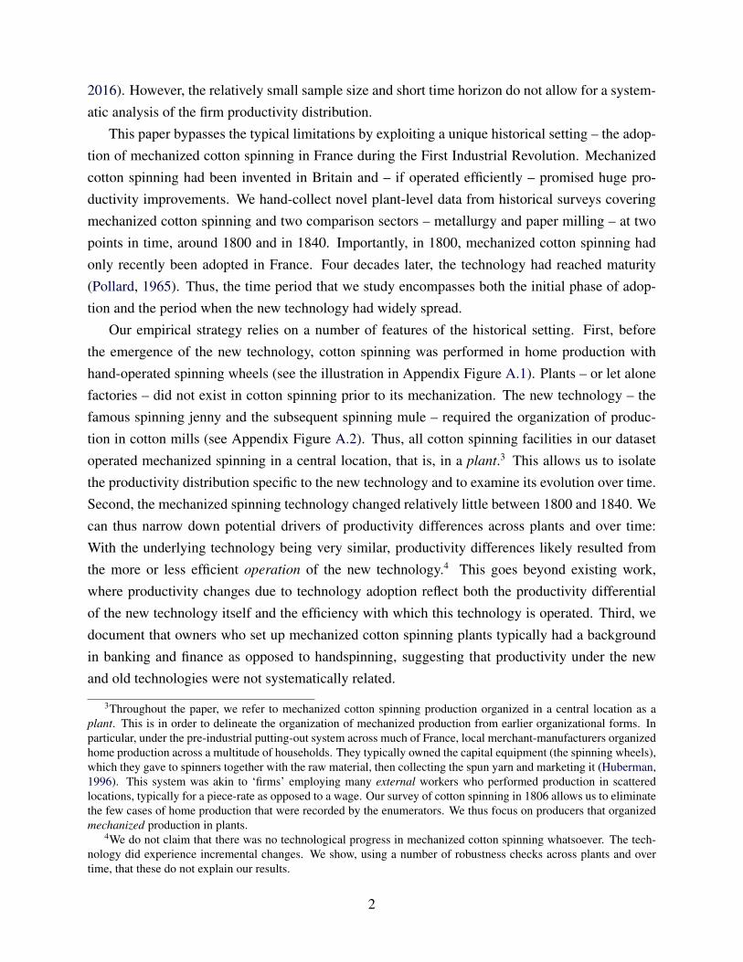
3.2 Industrial Census around 1840

The second period in our study is based on data from the first industrial census in France, conductedin 1839-47 and digitized by Chanut et al. (2000). For simplicity, we refer to these data as the ‘1840census.’ While this census covers all manufacturing establishments, we only use data for cottonspinning (528 plants), metallurgy (839 plants), and paper milling (348 plants).29 Figure 1 showsthe spatial distribution of plants around 1800 and in 1840 for the three industries.

The different surveys contain remarkably rich information, although the exact set of variablesvaries from survey to survey. Here, we discuss only the variables used across all sectors, as wellas additional, sector-specific variables when they are used in the empirical analysis. Our mainvariable of interest is labor productivity measured at the plant level and defined as the log ofrevenues per worker. We use this measure because it can be constructed for all sectors and in bothtime periods.30 Additionally, we are interested in estimating plant survival across the differentindustries over time. Given the importance of these variables for our analysis, we discuss the keyassumptions made in constructing them for each sector.

3.3 Constructing Plant Productivity

We face two challenges in constructing consistent productivity measures across plants and time.First, while the surveys for the three sectors around 1800 report output quantity (and some infor-mation on product-specific prices and quality), the census in 1840 directly reports plant-specificrevenues (but not output quantities). To render productivity measures comparable over time, wehave to construct revenues for 1800. Second, worker categories are not consistently reported acrossall plants in 1800 in metallurgy and paper milling. We discuss how we deal with each of these is-sues below.

28Juhász (2018, Appendix pp. 21-22) contains a detailed description of the cleaning process for these data. Of the626 entries, only 43 plants were dropped for these reasons. This is not because these types of production units were soinsignificant, but rather because the survey was not designed to capture them, so they were typically not enumerated.Note that the number of observations in Juhász (2018) differs substantially from that used in this paper, because theformer contains all plants active in the French Empire.

29One potential concern with the 1840 census is that plants with less than 10 workers may have been systematicallyunder-reported (Chanut et al., 2000). This is mostly relevant for paper milling, where plant size is the lowest. Inrobustness checks, we show that our baseline results hold even when only using plants with at least 10 workers in bothperiods.

30Our revenue-based productivity measure reflects both product prices and quantities. It is thus potentially affectedby changes in markups (Garcia-Marin and Voigtländer, 2019). However, this is unlikely to be quantitatively importantbecause all three sectors in our analysis produced standardized, often intermediate products.

15

Estimating Plant Revenues in 1800

In cotton spinning, the 1806 survey reports the quantity of yarn spun (in kilograms) as well as theminimum and maximum count of yarn spun, where the count of yarn is the standardized measureof quality in the sector.31 We construct plant-level revenue by multiplying the quantity of plant-level output by the price of the average quality of yarn produced by the plant. We use a scheduleof prices for different counts of yarn reported by the French government.32

In metallurgy, the 1811 survey asked for the quantity of output produced (by product) as well as theprice charged by the plant, by product type.33 While product-specific output quantity is reportedby all plants, the product-specific price is only reported by a subset of plants. We compute theaverage price for each product using the subset of plants where this information is available. Weobtain plant revenues by multiplying product-specific plant output by the average price for eachproduct and summing across products.

In paper milling, the 1794 survey reports the total quantity of paper products produced (in metricquintals), but it does not provide plant-specific output prices. To construct revenues, we multiplyplants’ output quantity with the average price of paper products produced in the correspondingdepartment, as reported in the Tableaux du Maximum – an extraordinary data source compiledin 1794 during the French Revolution that provides detailed data on goods prices and trade linksacross French regions. We use the department-specific price in order to accurately capture theproduct mix produced by plants in this area (see Appendix B.4 for detail). In robustness checks,we use the country-wide sectoral price.Price deflators Finally, to compare revenues in the earlier periods and in 1840, for all three sectors,we deflate revenue data using the producer price index (PPI) for the respective survey years fromMitchell (2003). Appendix B.5 provides detail on the underlying assumptions and approximationsin constructing these deflators. We note in passing that potential errors in the deflators wouldaffect our estimates for average growth rates in the three sectors between 1800 and 1840, but theywould not change the growth pattern across the plant distribution (e.g., the lower-tail bias in cottonspinning).

Constructing Consistent Labor Variables

In cotton spinning, the data provide consistent information on the number of workers employed bythe plant.

31We use the (unweighted) average of the minimum and maximum count of the yarn produced by the plant as aproxy for its average output quality. The maximum and minimum count is the only information that plants providedon the quality of yarn that they produced.

32Source: Document number AN F12/533 from the French National Archives. In robustness checks, we use a singlesector-level price, which we define based on the average quality of yarn produced across all cotton spinning plants.

33The survey includes the following products: iron of first quality, iron of second quality, iron of third quality, steelusing the cementation process, natural steel, and pig iron.

16

In metallurgy, about 40% of the plants reported both ‘internal’ and ‘external’ labor in the 1811survey, while the remainder of plants reported only total labor. Woronoff (1984, p. 138) describesexternal labor as only having very loose ties to the plant. These workers did not typically workat the location of the plant, their work was not supervised by the manager, and their identity wasoften not even formally known to the manager. They performed tasks such as driving, collectingcharcoal for the plant, or performing other jobs without belonging to the hierarchy or reporting tosuperiors in the chain of command. These types of workers were highly unlikely to be consideredformal salaried employees of the plant in the 1840 census. The challenge is thus to construct aconsistent measure of labor in 1811, given that approximately 60% of the observations report onlytotal labor, with no indication of whether this includes external labor. For these plants, we need anestimate of the size of their internal labor force. We use a nearest neighbor matching algorithm todetermine whether plants that only report total labor are more likely to be reporting internal laboronly or the sum of internal and external labor.34 When our algorithm suggests that the plant isreporting internal and external labor together, we estimate the number of internal workers by usingthe mean proportion of internal labor from all plants that report both types (the internal labor shareis 20%).

In paper milling, the vast majority of plants only reported male labor in 1794. We impute the totalnumber of employees in each plant by scaling male labor (reported by each plant) in 1794 by theaverage proportion of total employees to male employees in 1840 (where we observe both). Thevalidity of this method hinges on the assumption that the proportion of male employees remainedconstant over time. We are able to check this using the subset of plants that report all types ofworkers in 1794. We find that the proportions are remarkably consistent.35 Moreover, we showthat our results are robust to using only male employees in both periods.

3.4 Linking Plants over Time

It is possible to link plants over time given that all surveys report the name of the owner and thelocation up to the commune, which is the lowest administrative unit in France.36 We use two piecesof information to link plants over time: First, we match plants by their owner names in a givenlocation in the respective industry.37 Since the name of the owner may change even if the physicalstructure of the plant is the same, we also match by location in a second step: We match locations

34We match each plant that reports only total labor to its nearest neighbor that reports internal and external labor,where matching is based on capital, output, and the stage of production. We then classify a plant as “reporting onlyinternal lablor” (“reporting total labor”) if its reported total labor is closer to the matched plant’s internal labor force(internal plus external labor force).

35The proportion of total employees to male employees is 2.26 in 1794 for the subset of 20 plants that report alltypes of labor, while in 1840 it is 2.28 (among all plants).

36In bigger cities such as Paris, the arrondissement is also reported.37We use a fuzzy string match to allow for differences in spelling as well as for different first names of owners, in

cases where the plant was passed on within a family. Ambiguous matches were verified by hand.

17

where there is only one plant in the respective sector in 1800 and where there is at least one plantactive in the same sector in 1840. This turns out to be fairly common in the data. An obviousconcern is whether this ‘local matching’ indeed identifies the same plant. This is likely, given afortuitous feature across all three of our industries: their reliance on water power. Only a smallnumber of locations in a particular commune will be suitable for setting up a water-powered mill,as rapid stream flow is needed to yield sufficient power. Moreover, the backwater created by onemill means that another mill cannot be located in close proximity. Consistent with this, Crafts andWolf (2014) argue that agglomeration in the cotton textile industry was not observed until steambecame the common source of power in Britain. Consequently, our ‘local matching’ arguablyidentifies plants that have the same location within communes. Whether these were owned by thesame entrepreneur (or their descendants), or whether they had passed on to a different owner is notcrucial for our analysis.

One way to validate the assumptions underlying our ‘local matching’ is to examine how fre-quently communes with a single plant active in the sector in 1800 show up in 1840 with multipleplants active in the same sector. If this occurs frequently in the data, it would suggest that in factthere are multiple suitable locations for production in that sector for a particular commune. Thisis not the case in our data: For the vast majority of single-plant communes that we identify in theinitial period, there either continues to be one plant or no plants in the subsequent survey. It isexceedingly rare (6% of cases in both paper milling and cotton spinning, and 8% in metallurgy)across all three surveys for single plant communes to ‘add’ additional plants (despite the large in-crease in the overall number of plants in metallurgy and cotton spinning). As an additional checkon our methodology, it is also possible to compare plant survival in metallurgy to that reported inWoronoff (1984) for this sector over the period 1788-1811. If our strategy of ‘local matching’ ledto too many plant matches over time, we would expect an exaggerated survival rate. The contraryis true: Our estimates of plant survival rates for the period 1811-1840 are well below (one halfor less) those that we calculate for the period 1788-1811. This suggests that it is unlikely that wesystematically overestimate plant survival.

3.5 Plant Survival Rates

Our main measure of plant survival is based on the combination of matching by owner name and‘local matching’ that we described above. We define the survival rate as the percentage of plantsfrom the initial period that survive into the later period. The numerator counts all plants that fulfillat least one of the following two conditions: i) the plant has the same owner in both periods; ii)there is only one plant in the respective sector in the location in the initial period and at least oneplant in the same sector in 1840. The denominator is the sum of all plants in the given sector inthe initial period. Note that this rate does not adjust for the fact that the number of plants located

18

in communes that have only one plant varies across the three sectors in our sample.38 Thus, wemay mechanically find higher survival rates in a sector where single-plant communes are relativelymore frequent. To address this issue, we also construct the ‘restricted sample’ survival rate as arobustness check. This measure is based solely on single-plant locations. The numerator countsthe number of communes that had only one plant in the respective sector, in both the initial periodand in 1840 (indicating plant survival). The denominator counts the number of communes thathad a single plant in the respective sector in the initial period and either one or no plant in 1840(indicating plant survival and plant exit, respectively).39

4 Empirical Analysis

In this section, we use our data to study the evolution of the plant size and productivity distributionin mechanized cotton spinning after the new technology had been adopted. We contrast the patternsin cotton spinning to those observed in two comparison sectors – metallurgy and paper milling.After documenting our main result, we propose and investigate a mechanism that can rationalizethe observed patterns. Finally, we consider a set of alternative mechanisms that could account forthe results and test them empirically.

4.1 The Evolution of Plant Scale

What did plants look like in 1800 across the three sectors, and to what extent did they undergochange during our study period? Table 2 provides an overview, reporting the evolution of plantsize, measured by the number of workers. A few points stand out. First, as early as 1806, cottonspinning plants were strikingly large. The average spinning plant in this period had 63 employees(the median was 30).40 Despite the recent introduction of mechanized cotton spinning in France,plants were already much larger than in the two comparison sectors, which had a much longertradition of factory-based production: Plants in metallurgy (reported in 1811) had on average 20workers; paper milling plants had on average 13 employees.41 In sum, despite the late start of

38Among the 593 plants in paper milling in 1794, 218 (36.8%) were the only plants active in their commune in thissector. For cotton spinning in 1806, the proportion is 25.4% (99 out of the 389 plants), and in metallurgy in 1811, 69%(329 out of 477 plants).

39Based on this sample definition, we exclude plants that were the only ones in their commune in 1800, and wherethere was more than one plant in 1840. As discussed above, the number of these “uncertain” observations is very smallacross all sectors, which we consider a validation of our methodology.

40Recall that mechanization, which triggered the move to factory-based production, was invented only in the late18th century. Moreover, the machines were only adopted sporadically across France prior to the 1800s. Consistentwith these facts, the median plant in cotton spinning was three years old in 1806.

41One caveat with making this comparison is that the paper milling survey dates from 1794. Thus, plant size mayhave grown by 1806 – the year of the cotton spinning survey. In addition, we had to extrapolate the overall numberof workers in paper milling in 1794 (including women and children – see Section 3.3). However, it is unlikely thattrue plant scale would have been very different in 1806. This is because even in 1840, the average plant size in papermilling was only 43 (including women and children, which are reported in this year). We can thus be confident thatpaper milling plants in 1806 were substantially smaller than cotton plants. Finally, there is a concern that the 1840census did not enumerate all plants with less than 10 employees. Table D.13 shows that plant scale increased across

19

factory-based production in cotton spinning, the average plant was large compared to other sectorsalready at the turn of the 19th century.42

Table 2 also shows that all sectors underwent significant growth in plant size over the period1800-1840. Average plant size doubled in cotton spinning and grew threefold in the other two sec-tors. In 1840, the average cotton spinning plant had 112 employees (median 72), while metallurgyand paper milling had 57 and 43 workers on average, respectively. The level and increase in plantscale is consistent with Sokoloff’s (1984, Table 1, p. 5) findings for the United States using estab-lishment level data from the 1820 and 1850 manufacturing censuses. The data for the US cover 10industries. Similar to our data for France, the US data include both mechanizing sectors (such ascotton textiles) and non-mechanizing sectors such as tanning.43 While their coverage is richer, theUS data are less suitable for isolating productivity changes in mechanized cotton spinning over theearly phase of industrialization. The reasons are twofold: First, there was no handspinning tradi-tion before mechanization in the US, so that local input and output markets had to be established atthe same time as plants (Ware, 1931). This is prone to lead to differences in local production costsand markups, thus affecting (revenue-based) productivity estimates (Garcia-Marin and Voigtlän-der, 2019). Second, the US coverage begins at a later point in time, in 1820, when mechanizationwas already well underway (Ware, 1931).

4.2 The Pattern of Productivity Growth

Next, we examine the evolution of plant productivity in France during the first decades of the19th century. We begin by examining average annual labor productivity growth. Column 1 inTable 3 shows that all three sectors experienced a significant increase in labor productivity. Thelargest productivity gains were achieved in cotton spinning (2.4% per year), followed by metallurgy

all three sectors even when we limit the sample in both years to only include plants with more than 10 employees.42Granted, our data only cover two comparison sectors. However, these two sectors had a long tradition of factory-

based production and relied on high fixed-cost capital as well as inanimate power sources. This makes it likely thatmetallurgy and paper milling plants had relatively large plant size, as compared to plants in other sectors around 1800for which we do not have data. We can also use the 1840 Census, where we know the size of plants in all other sectorsto gauge support for this assertion: The average plant size in cotton spinning in 1840 is in the 85th percentile of allplants, while both metallurgy and paper plants are in the upper tercile of the plant size distribution across all sectors.In addition, all three sectors belonged to the top 90th percentile in terms of the share of plants using “any power,”where the 81 sectors in the census are ranked by the share of plants using inanimate power sources.

43For comparison, the average size of cotton textile establishments was 34.6 in the US in 1820 and 97.5 in 1850.Similar to France, but based on a larger set of comparison sectors, cotton textiles was the biggest in terms of plantscale already in 1820. The one exception to this is glass-making, but Sokoloff (1984) urges those numbers to betreated with caution as they are based on a sample of only 8 establishments. “Iron and iron products” in the US had19.5 and 24.2 employees in the two periods, respectively, while paper milling had an average of 14.3 and later, 22.4employees. Since employment and productivity grew in both mechanizing and non-mechanizing sectors, Sokoloff(1986) concluded that mechanization itself cannot be the only driving force behind these trends. Our findings for theFrench sectors support this conclusion and add the additional finding that even after the initial adoption of mechanizedspinning, productivity and plant size grew substantially.

20

(1.9%) and paper milling (0.7%).44 Remarkably, the estimated productivity increase is largest inspinning, despite the fact that all plants in this sector already used the new technology in 1800. Inother words, because we only compare plants that used mechanized cotton spinning, the observedproductivity increase must be due to efficiency gains within the new technology. This is in contrastto the two comparison sectors, where innovations replaced older technology vintages in existingplants – most prominently, coal as an energy source in metallurgy, and the Foudrinier machinein paper milling (which mechanized the formation of paper). Thus, labor productivity growth inthose sectors reflects not only improvements in operating existing vintages, but also gains from theadoption of new technology vintages.

In which part of the productivity distribution were these gains concentrated? Figure 2 plotsthe distribution of labor productivity in the three sectors at the beginning and at the end of oursample period, illustrating our main results. In cotton spinning, two features stand out. First,the initial dispersion in labor productivity was large in 1800 relative to that in 1840. Second, theproductivity gains are almost exclusively concentrated in the lower tail – the lower tail disappearedover our sample time period, while increases in productivity at the upper tail were modest. Thecontrast between cotton spinning and our two comparison sectors is striking. In metallurgy andpaper milling, the entire productivity distribution shifted to the right between 1800 and 1840.Quantile regressions confirm this pattern. Columns 2-6 in Table 3 report these results for the threesectors, estimating regressions for productivity growth at different quantiles of the productivitydistribution. Figure 3 displays the corresponding coefficients. In cotton spinning, the bias towardsproductivity growth in the lower tail is striking. Productivity growth at the 25th percentile wastwice as large as that at the 75th percentile (3.3% per year relative to 1.65%), and the difference ismore than fourfold between the 10th and the 90th percentile (3.9% and 1.0%, respectively). In thecomparison sectors, the differences are more modest across the distribution; if anything, growthwas concentrated in the upper tail: In both metallurgy and paper milling, the productivity growthat the 25th percentile was marginally lower than at the 75th percentile.

Could the different pattern in cotton spinning be driven by output quality? Recall that our dataenable us to use quality-adjusted prices in 1800 for cotton spinning, while quality adjustments arenot possible in the two comparison sectors. Panel B in Table D.1 in the appendix presents quantileregressions without quality-adjustments, i.e., using the same sector-level price across all plants incotton spinning. The magnitude of the lower-tail bias is slightly smaller, but it remains striking.

44Given that we discount revenues using price indices, all our productivity calculations reflect price-adjustedrevenue-based productivity. To obtain the average annual growth rates between the two time periods (around 1800and 1840), we first regress log output per worker ln(Y/L) on a dummy for 1840 in each sector. This coefficientmeasures the percentage growth in output per worker over the entire time period between the respective survey years.We then annualize these values (and corresponding standard errors) by dividing by the number of years between thesurveys in each sector. Note that this method delivers average annual growth figures, not accounting for compoundgrowth. In cotton spinning, the overall growth over the period 1806-40 amounts to 82% (2.42% per year x 34 years).

21

The difference in productivity growth between the 10th and the 90th percentile is 3.4% relativeto 1.6%. Thus, differential trends in output quality do not drive the observed differences in theproductivity distributions across the three sectors.

Our baseline productivity measure is log output per worker. For cotton spinning, we can alsocompute TFP, using detailed data on physical machinery (number of spindles) – see AppendixD for detail. Panel C in Table D.1 confirms the lower-tail bias of productivity growth in cottonspinning using TFP. Table D.2 presents additional robustness checks on data choices we havemade in the paper milling industry. We show that our quantile regression results in paper millingare robust to i) using only male labor and ii) to pricing output in 1794 using the country-wideaverage price as opposed to the departmental price used in the baseline analysis.

Summing up, the results in this section show that after the adoption of the new technologyin mechanized cotton spinning, the industry witnessed major increases in productivity that weredriven by a disappearance of the lower tail of the productivity distribution. Over time, the plantproductivity distribution became less dispersed. This is in contrast to the patterns observed in thecomparison sectors, where mean productivity growth was more modest and occurred relativelyevenly across the productivity distribution.

4.3 Proposed Mechanism: Learning About Best Practice in Factory-Based Production

What explains the lower-tail bias of productivity growth in mechanized cotton spinning? The his-torical narrative points to an important role of learning about the efficient organization of factory-based production and adequate handling of new machinery. As documented in Section 2, earlyadopters in cotton spinning needed to engage in trial and error along multiple dimensions. Thisinvolved the development of best-practice methods for operating the new technology efficientlyand integrating it into other, similarly new aspects of factory-based production.

A Stylized Framework. We formalize this process in a simple stylized framework that gives rise tolower-tail biased productivity growth. We summarize the key features here; Appendix C presentsthe model and shows simulation results. The essential ingredients are: i) a production function thatinvolves multiple complementary inputs (tasks); ii) independent, random draws in the efficiencyassociated with each input; and iii) the lower bound of each input’s efficiency draw increases overtime (i.e., very bad draws disappear).

In cotton spinning, initially, very low input efficiency draws are possible. The complemen-tarity across inputs implies that a low efficiency draw for only one input diminishes output sub-stantially.45 This gives rise to a fat lower tail of the productivity distribution. Over time, we letthe lower bound for the input efficiency draws in cotton spinning increase. This reflects improvedknowledge about organizing and handling each input – either due to learning within plants or due

45In the extreme complementarity case – a Leontief production function – output drops in proportion to the mini-mum efficiency draw, no matter how large the draws for the other inputs are.

22

to knowledge diffusion across plants.46 At the same time, we assume that the upper bound forinput efficiency draws does not change, i.e., the technological frontier in mechanized cotton spin-ning remains the same. Intuitively, learning (within plants or from other producers) eliminates theworst mistakes in organizing production; but the best possible draws remain unchanged becausethe underlying technology does not change. This setup leads to productivity growth concentratedin the lower tail. Figure C.1 in the appendix illustrates the simulated productivity distributions.47

The left panel of Figure C.1 shows the resulting evolution of the plant productivity distributionover time: The initially fat lower tail disappears in the second period – intuitively, very bad drawsthat pull down output towards zero (even if all other draws are high) have been eliminated. Thisproductivity pattern mirrors the one for cotton spinning in the data (see Figure 2).

We also adapt our simulation to the comparison sectors. Since plant-based production in thesesectors was already well-established around 1800, we choose a higher lower bound to reflects thatlearning had already occurred. To represent the incremental technological progress that improvedthese technologies over time, we shift both the upper and lower bound outward in the secondperiod. The corresponding simulation results are shown in the right panel of Figure C.1. Theyresemble the pattern observed for our control sectors, metallurgy and paper milling, where thewhole productivity distribution shifted to the right.

While this stylized theoretical framework is not the only one that gives rise to lower-tail bias inproductivity growth, it is a simple setup that represents the key features of the historical evidence.In what follows, we use this stylized framework to guide our discussion of possible mechanisms.

Plant Survival Across the Sectors. The historical evidence discussed in Section 2 suggests thatlearning best-practice methods was an important dimension during the shift to factory-based pro-duction in cotton spinning. We now provide evidence that this mechanism can explain the observedplant productivity patterns. First, we examine plant survival across sectors. If early adopters ofmechanized cotton spinning technology had to experiment with best-practice methods, we wouldexpect initially low plant survival rates relative to the other two sectors. Experimentation wasarguably costly. For example, the layout of the factory was to a large extent a sunk investment.Changes and extensions could of course be made, but at substantial cost. Thus, initial design flawswere hard to correct and likely led to exit. Indeed, we find evidence of substantially larger exitrates in cotton spinning relative to the other two sectors. Table 4 reports plant survival rates overour sample period, using the two measures defined in Section 3.5 in each of the three sectors.Based on our baseline measure, survival rates in spinning (7%) were slightly lower than in paper

46While our stylized theory is agnostic as to which of these mechanisms dominated, the empirical results belowsuggest that the diffusion of organizational practices across plants was an important dimension.

47We use a CES production function with three inputs and choose the elasticity of substitution across inputs tobe 0.5, indicating a strong degree of complementarity. Efficiency in each of the inputs is drawn from a uniformdistribution with support [0, 1]. Over time, the lower bound for each distribution increases to 0.1.

23

milling (9%) and much lower than in metallurgy (34%). Note that the paper milling survey wasconducted in 1794, more than 10 years earlier than the cotton spinning survey (1806). If we ad-justed for the longer horizon in paper milling, the implied survival rates for 1806-1840 would besignificantly higher. This implies that the differences in survival rates between cotton spinning andpaper milling are probably higher than reflected in Table 4.

Turning to the ‘restricted sample’ survival rates, the differences across the three sectors are evenstarker. By this measure, the survival rate in spinning is still about 7%, but it is much higher in thecomparison sectors: 20% in paper milling and 49% in metallurgy. Recall that this second survivalrate is based on single-plant locations. Thus, the low survival rate observed in cotton spinningmeans that many locations lost their (only) cotton mill. This is consistent with a mechanism inwhich owners that invested in a cotton spinning mill with poor layout had to exit the market, andthe structure of the mill was not subsequently used by other firms in cotton spinning.48

Plant Exit and Productivity. In Table 5 we examine the extent to which plants that eventuallyexited the market by 1840 had lower initial productivity around 1800, as compared to survivingplants. This pattern is strong in cotton spinning, where churn was the highest: Exiting plants were53% less productive than survivors, and this difference is highly statistically significant. Exitingplants were also less productive in the comparison sectors, but there, the pattern is less pronounced:exiting plants were about 15% less productive in both sectors, and this number is not statisticallydifferent from zero. Columns 2 and 3 in Table 5 also show that exiting plants were significantlysmaller, both in terms of employees and output, and that this pattern is particularly pronounced incotton spinning.

Overall, we find that exiting plants in cotton spinning were particularly unproductive comparedto survivors, and – likewise – the survival rate was significantly lower than in other sectors. Thesefindings – in combination with the widely dispersed productivity distribution in cotton spinning –are consistent with large organizational challenges and low initial guidance in switching to factory-based production in cotton spinning.

Age Profile of Plant Productivity. Next, we examine whether the age profile of plant productivityis consistent with a mechanism of learning best-practice methods. We expect younger plants tohave higher productivity, because they had a larger set of previously established plants from whomthey could learn. We exploit the richness of our data to test this in both 1800, when best practicemill design was still evolving, and in 1840, when according to Pollard (1965), the industry hadreached maturity – at least in Britain. The 1806 survey in cotton spinning contains the year of

48Lower survival rates in spinning could also be consistent with the fact that the industry moved towards steampower to a larger extent than other sectors and hence moved away from water power. However, note in Table D.3 thateven in spinning, steam power seemed to be used in addition to water power: 66% of cotton spinning plants still usedwater power as a source in 1840. Moreover, cotton mills using steam power were somewhat less productive (see TableD.4), suggesting that in France plants did not face a strong profit incentive to move away from water power.

24

foundation of plants. This allows us to compute a dummy for ‘young’ plants, defined as below-median age (with the median age in 1806 being three years). We first examine whether plant ageis systematically correlated with productivity in cotton spinning. Column 1 in Table 6 shows thatthe unconditional association is strongly positive: ‘Young’ plants were 58% more productive in1806. This could be driven by mechanisms other than the one we examine. For example, newentrants may have used the most recent vintage of capital, leading to higher physical productivity(Foster, Haltiwanger, and Syverson, 2008). To address this issue, we control for several importantplant characteristics in columns 2-7 of Table 6. These include the average quality (count) of theyarn spun, the capital intensity of the plant (measured as log spindles per worker), the number ofworkers in the plant, and the vintage of machinery (a binary variable for using different vintages ofmachinery – these are not mutually exclusive categories)49 The coefficient of interest remains largeand highly significant when we add these controls one-by-one.50 The only control that notablychanges the magnitude of the coefficient of interest is the quality of yarn (column 2). However, thequality of the yarn that a plant could spin partly reflected its level of learning, and is thus arguablyalso capturing our mechanism. This is because the quality of yarn that could be spun by a plantdepended on the quality of the machine and the precision of its operation (Huberman, 1996). This,in turn, may have reflected improvements of the machinery achieved by tinkering, and the acquiredskill of the spinners, both of which are a central part of our learning mechanism.

Next, we turn to the productivity-age pattern in 1840. While the data for this second period aregenerally more comprehensive, we do not observe plant age. However, we can perform a similar– albeit weaker – test based on the comparison of surviving and entrant plants: In Table 7 weregress log output per worker on an indicator for whether the plant was an ‘entrant’ in 1840 (asopposed to a surviving plant by our definition from Section 3.5). The coefficient on the ‘entrant’dummy thus reflects the average productivity differential for plants that entered between the initialsurvey year (1806) and 1840. Best-practice mill design evolved over this period, and it had largelyconverged by 1840 (Pollard, 1965). Correspondingly, we find that ‘young’ plants were not moreproductive; the coefficient is in fact negative, but not statistically different from zero. This holdsalso when we control for the use of water power, steam power, any other power source (wind oranimal power used by a small subset of plants), and for the number of workers. We perform anadditional exercise in the appendix, using data on metallurgy plants in both periods (Tables D.5and D.6). For this sector, in both periods, the best measure of plant age that we observe is a binaryindicator of plant survival from 1788 to 1811, and for survival from 1811 to 1840 (the latter beingthe same procedure as for cotton spinning in Table 7). Overall, the results do not point to youngerplants in metallurgy having a strong productivity advantage: In 1811, ‘young’ metallurgy plants

49The three different vintages of machinery are the spinning jenny, the throstle, and the mule-jenny.50We do not include all controls together because of multicollinearity concerns.

25

were only marginally more productive, and in 1840 ‘young’ metallurgy plants were somewhat less

productive.51

Spatial Diffusion of Knowledge. In what follows we shed light on how the learning process tookplace. The historical background discussed in Section 2 suggests that plants copied successfuldesigns and setups of the production process from each other. To examine this channel, we estimatewhether a plant’s own productivity was higher in the proximity of other high-productivity plants.We use the following specification:

ln(Y/L)ij = β0 + β1Distp90ij + FEj + εij ,

where ln(Y/L)ij is labor productivity (log output per worker) for plant i located in departmentj; Distp90ij is log distance to the nearest plant (in the same sector) with productivity in the 90thpercentile (in the distribution of all plants in the sector across France). Plants that are themselvesin the top productivity decile are excluded from the sample to avoid introducing a mechanical rela-tionship. Our preferred specification includes department fixed effects (FEj) to absorb unobservedlocation characteristics that may make all plants in a given region more productive, irrespective oflocal spillovers. Thus, the coefficient of interest β1 reflects the extent to which plants in the samedepartment benefit from being located closer to a high-productivity plant (which may be located inthe same or in another department). We do not interpret these correlations as causal effects, but asevidence that is compatible with spatial spillovers of production knowledge. We estimate the spec-ification separately for the three sectors, and in both time periods. Standard errors are clustered atthe department level to account for spatial correlation.

Before presenting the results, we first examine the spatial distribution of high-productivityplants across our sectors and time periods. Figure D.1 in the appendix plots the spatial distributionof cotton spinning, metallurgy, and paper milling plants, distinguishing those in the 90th percentileof the productivity distribution. Unsurprisingly, some regions have a larger concentration of high-productivity plants than others, but there are no marked differences in this pattern across the threesectors or over time. Since we exploit within-department variation in distance to high-productivityplants, the cross-regional differences in the concentration of high-productivity plants do not affectour results.

Figure 4 visualizes our baseline results on spatial diffusion, and Table D.7 in the appendixreports the corresponding regressions. To allow for direct comparability, we report the standardizedbeta coefficients of Distp90 for all three sectors in the two periods. The estimated coefficient for

51In metallurgy in 1811, ‘young’ plants were 22% more productive when no controls are added (as compared toalmost 60% for the same specification in cotton spinning). Once we control for plant size (log workers) in column 2in Table D.5, the productivity advantage disappears. Note that the metallurgy survey has sparser information on thisdimension; plant size is the only control that can be added in 1811.

26

cotton spinning in 1806 is negative, statistically significant and large in magnitude: A one standarddeviation increase in distance to a high productivity plant in the sector is associated with a 0.81standard deviation decline in labor productivity. The pattern is much weaker in the two controlsectors, metallurgy in 1811 and paper milling in 1794 – the coefficients are less than one-third inmagnitude as compared to cotton spinning. In addition, in 1840, there is essentially no relationshipbetween labor productivity and distance to top-plants in any of the three sectors. Thus, proximityto high-productivity plants mattered the most in cotton spinning in 1806, i.e., in the sector thatsaw the most dramatic change during industrialization, and in the period before knowledge aboutthe optimal organization of production had spread widely. While this pattern is consistent with alearning mechanism, it could also be driven by a number of other forces. We turn to examiningpossible alternative explanations below.

While department fixed effects capture unobserved differences that vary at the department level,they cannot capture unobserved differences at a finer spatial level. To test for these, we use fourapproaches. First, we control directly for some prominent location fundamentals at the communelevel such as the availability of fast-flowing streams (as a source of water power), proximity tocoal (which matters for steam power), and the share of forest cover (which matters for accessto charcoal – a major input in metallurgy).52 Table D.8 in the appendix shows the results forspecifications that control for all of these location fundamentals. The pattern of the coefficients ofinterest does not change, and the estimated magnitudes remain very similar. Moreover, the locationfundamentals themselves are mostly small and statistically insignificant. This is probably driven bythe fact that the department fixed effects already account for the most important spatial differencesin location fundamentals. Second, our results could be affected by more general agglomerationexternalities, as opposed to learning. In particular, our findings may be driven by high-productivityplants emerging (within departments) where the density of production is large due to agglomerationforces. We investigate this explanation directly by adding a control for the density of productionat the commune level (measured as the log of total output in the sector, excluding a plant’s ownoutput). Table D.9 in the appendix shows that controlling for the local density of production barelyaffects our results: The estimated coefficient on distance to high-productivity plants in cottonspinning in 1806 decreases by about 10% to -0.74 (se 0.19), while the distance coefficients in theother sectors and in 1840 remain relatively small. The coefficient on local production density itselfis generally small, positive, and never statistically different from zero.

Appendix Table D.10 presents our third approach to probe for unobserved location fundamen-

52The sources for these data are as follows. Data on the stream flow of rivers are from EURO-FRIEND (http://ne-friend.bafg.de/servlet/is/7397/). These data report water flow rates from thousands of geocoded collection pointsacross France. Data on charcoal sources are from the highly detailed ‘Cassini maps’ produced in the late 18th centurythat contain information on forest cover. These maps were geo-referenced by Vallauri, Grel, Granier, and Dupouey(2012). Finally, data on the location of coal deposits – both in France and near its borders – were geo-referenced frommaps in Tarr and McMurry (1993) and Guiollard (1993).

27

tals (within departments). We conduct a placebo exercise that examines whether plant productivityin 1800 was also related to the distance to high-productivity plants that only emerged later, i.e.,plants in the top-90th percentile of productivity in 1840. Reassuringly, the estimated coefficient incotton spinning is close to zero and statistically insignificant. In other words, productivity in cottonspinning in 1806 was not related to high-productivity locations three decades later. This suggeststhat the large estimated coefficient in our baseline specification is not driven by persistent locationfundamentals within departments.

Finally, we examine the extent to which the estimated distance coefficient in cotton spinning in1806 may be driven by plant selection. It is possible that we estimate a large (negative) coefficientin cotton spinning in 1806 not because plants were learning from their high-productivity neighborsbut rather because ex-ante high-productivity plants selected into ‘productive locations’ (i.e., choseto locate near existing high-productivity plants). Given that we observe plant age in cotton spinningin 1806, we can examine selection patterns, building on our findings from Table 6 that ‘young’plants in cotton spinning were particularly productive. In Table 8, we show that our coefficientof interest is robust to controlling for log plant age (column 1) and to adding the interaction ofplant age and distance to high productivity plants (column 2). This suggests that (conditionalon department fixed effects) plant entry did not vary systematically with the location of high-productivity plants. A different, arguably more conservative approach is to estimate the coefficientof interest using only the subsample of plants that entered before the nearest high-productivityplant. The timing of entry of these plants rules out systematic selection. In column 3 of Table8 we show that the coefficient on distance to high-productivity plants remains statistically highlysignificant, although it is somewhat smaller than in the baseline sample (-0.44, se 0.153). Columns4 and 5 show that the coefficient of interest remains stable and statistically significant as controlsfor plant age and the interaction between plant age and distance to high-productivity plants areadded in this subsample.

In summary, the consistently larger distance coefficient estimated in cotton spinning in 1806,in combination with a series of robustness checks, points to the spatial diffusion of knowledge asone mechanism through which learning across plants took place.

4.4 Robustness to Alternative Explanations

In the final part of this section we consider potential alternative mechanisms that could explainour results. Recall that we observe the lower-tail bias in productivity growth only in cotton spin-ning, and not in the other two sectors. This suggests that the mechanisms driving the effect areeither specific to cotton spinning or they affect this sector differentially. Below, we consider somecompeting mechanisms that would fit this pattern.

Market Integration. Could increased market integration explain our results in cotton spinning? Asthe French economy became more integrated over time, it is possible that lower-productivity plants

28

faced tougher competition and had to exit the market.53 However, we do not observe a lower-tailbias in productivity growth in the two comparison sectors. Thus, for market integration to explainour results, it must have affected the cotton sector differently.

We first note that the exit pattern in Table 5 speaks against such a mechanism: If marketintegration increased particularly strongly in cotton spinning, we would expect even relativelyproductive plants to exit the market, because of an increased productivity threshold that allowsfor profitable production (Melitz, 2003). However, the contrary is true: Exiting plants in cottonspinning had a particularly low productivity, as compared to the other two sectors.

Second, data on market integration also speak against a confounding role of this channel. Cot-ton yarn (and textiles more generally) are high value-to-weight products, which makes them moreeasily tradable over long distances than iron or paper. This suggests that cotton spinners may al-ready have faced tougher competition through more integrated markets in the early 1800s. Thus,we would not necessarily expect cotton spinning to be the most affected sector by increased mar-ket integration after 1800. Consistent with this reasoning, we present evidence for relatively highmarket integration in cotton yarn in the late 18th century. We use data in 1794 from Daudin (2010)on the number of districts across France that reported consuming cotton textiles, iron, or paperproducts from any district in a given department.54 Intuitively, higher market integration meanslower price differentials across departments, which in turn implies that highly productive areascould dominate the market throughout France. Consequently, we can infer high market integrationfrom the data if we observe that a few (presumably highly productive) departments sold to manyother departments, while the majority of departments produced no output, or did so only for localconsumption. Figure D.2 in the appendix shows that this pattern is particularly strong in cottontextiles. Many departments produced mostly for themselves if at all (these are the zeros and ones),while a few departments supplied cotton to a large number of districts. The top tercile of depart-ments exported cotton textiles to 30 or more districts. In the two comparison sectors, there is lessspecialization and less evidence for market integration: Fewer departments report not supplying toanyone (particularly in paper), and the top decile of departments supplied only to 6 (paper) and 7(iron) districts in total. This suggests that cotton textile plants were already competing in a biggermarket than the comparison sectors around 1800.

The appendix presents two further robustness checks that probe the extent to which marketintegration may explain our results. We introduce two controls in our quantile productivity regres-sions (see the baseline results in Table 3). Table D.11 controls for market potential, and Table

53Market integration arguably increased during our sample period both for policy reasons such as the abolition ofinternal barriers to trade during the French Revolution (Daudin, 2010), and because of infrastructure improvementsthat reduced transport costs such as the introduction of railways in the late 1820s.

54Districts are administrative units that stayed in place for approximately five years, from 1790 to 1795 – with eachdepartment including from a minimum of 3 to a maximum of 10 districts.

29

D.12 introduces region fixed effects.55 Controlling for market potential changes the coefficientsof interest only marginally, while adding region fixed effects dampens the lower-tail bias in cottonspinning: Productivity growth at the 10th percentile is now only twice as large as in the 90th per-centile (as compared to a factor of almost 4 in the baseline regressions in Table 3). This suggeststhat a part of the pattern is driven by reallocation across regions, but not in a way systematicallyrelated to market potential.

Plant Size and Early Spinning Workshops. Another potential concern is that our results may bedriven by the disappearance of small cotton spinning plants (or ‘workshops’). While our baselinesample filters out small establishments that used handspinning wheels (see Section 3.1), it mayinclude relatively small plants that operated early vintages of mechanized spinning jennies that didnot necessarily need inanimate sources of power. This small-scale setup may have been inherentlydifferent from the larger-scale factories powered by inanimate power sources. While the move tofactory-based production was swift, systematic differences of smaller mechanized cotton work-shops could account for the lower-tail bias of productivity growth in this sector. Our data does notdifferentiate between these two types of plants (we observe the capital vintage, but not the powersource in the 1800 data). However, we can examine the extent to which our results could be drivenby these forces in a number of ways.

One way to examine the influence of smaller plants on our results is to adopt a stricter definitionof ‘factory-production’ and use only those plants that have more than 10 employees. This shouldexclude the majority of the smaller workshops that may have been organized as factory-basedproduction along some but not all dimensions. Figure D.3 and Table D.14 in the appendix showthat the lower-tail bias in productivity growth is robust to using only larger plants. The magnitudesremain similar at most quantiles, while the lower-tail bias of productivity growth remains uniqueto mechanized cotton spinning. These findings also address the concern that smaller plants mayhave been under-sampled in 1840.

Next, we implement an even more conservative definition of factory-production. We drop anyplant from the 1806 survey that reports using the earliest vintage of machinery – the spinningjenny. These were the types of machines that could, in principle, have been operated also in smallworkshops without inanimate power sources. While the introduction of spinning jennies – evenin workshops – would have faced challenges in re-organizing production, dropping them fromthe survey allows us to assess the extent to which these may have driven the lower-tail bias ofproductivity growth. Table D.15 contains the quantile regression results. The lower-tail bias ofproductivity growth remains striking. Thus, it is unlikely that early spinning workshops that share

55Market potential is computed as the sum of inverse distance-weighted city population in 1800. Regions are largerthan departments: There are 22 regions in France and 86 departments. Our data in the three sectors do not haveenough observations to include department fixed effects, i.e., to estimate meaningful productivity distributions withindepartments.

30

some, but not all features of factory-based production drive the lower-tail bias of productivitygrowth.

Finally, our results could also be driven by increasing plant scale. Recall, however, that this isunlikely, as all sectors witnessed an increase in plant scale. Indeed, as the results in Table D.16show, controlling for the number of workers in each plant does not alter our findings.

Effects of the Napoleonic Blockade on the Cotton Spinning Sector. Juhász (2018) shows that tem-porarily higher trade protection from British competition shifted the location of the mechanizedcotton spinning industry within France. To what extent does varying trade protection explain thelower-tail bias of productivity growth in cotton spinning? This is unlikely, given that our resultshold within regions, where the pattern of protection was very similar (see Table D.12). FigureD.4 presents further evidence that varying trade protection does not drive our results, by splittingthe sample into plants in northern and southern regions in France (corresponding to the main di-mension along which protection varied). The productivity distributions in the north and south areremarkably similar, and in both regions, productivity growth until 1840 was due to a disappearinglower tail.

Could the blockade explain the lower plant survival rates observed in cotton spinning relative tothe other sectors? In Table D.17 we split mechanized cotton spinning plants into the same northernand southern regions and report survival rates separately. Indeed, consistent with Juhász (2018),survival rates are lower in the south than in the north (which experienced a relative increase intrade protection during the blockade). However, survival rates remain low relative to the other twosectors even when we narrow our sample to only northern plants.56 This suggests that an importantpart of low survival rates in mechanized cotton spinning are not driven by the uneven effects of theNapoleonic blockade across France.

Improvements in the Technology. Another possible alternative mechanism is that productivitygrowth in cotton spinning was driven by technological improvements of the mechanized machin-ery after 1800. This is unlikely for two reasons. First, as we discussed in Section 2.1, the vintagesof capital in cotton spinning remained largely unchanged during our sample period. Second, it isunclear why the successive adoption of better capital vintages would be concentrated in the lowertail of the plant-productivity distribution. In fact, in our two comparison sectors – where newvintages became available – the whole distribution shifted to the right.

In Table D.18 we examine whether capital deepening can account for our results by controllingdirectly for the capital-labor ratio of the plant (measured as the number of spindles per employee).

56Note that the raw baseline survival rate for northern plants is now slightly higher than in paper milling (11%and 9%, respectively). Recall, however, that the cotton spinning survey was conducted much later than paper milling(1806 as opposed to 1794). Moreover, the restricted sample survival rate in the north is half that measured in papermilling (10% and 20%, respectively). Taken together, this suggests that even comparing only cotton spinning plants inthe north of France to the comparison sectors (calculated for all of France), survival rates for northern cotton spinningplants were low.

31

The lower-tail bias for productivity growth remains robust and similar in magnitude, suggestingthat neither differential capital deepening nor changes in the vintages of capital drive our results.57

In sum, our results are unlikely to be driven exclusively by technological improvements over timethat were accessible to all plants.

Quality Upgrading. We assess the extent to which the lower-tail bias in mechanized cotton spin-ning could be driven by quality upgrading across plants over time. The concern is that if plantsshifted their product mix to higher-quality products over time (or more precisely, plants producinghigher-quality yarn entered the market), this could explain our result. We have no way of directlytesting for this because we do not observe any information about the quality of output produced inthe 1840 census. However, we can use our data in 1806 to examine the extent to which plants pro-ducing low quality account for the fat lower tail in that period. Unsurprisingly, quality is positivelycorrelated with our measure of labor productivity (see column 2 in Table 6). However, quality doesnot account for a significant part of the lower-tail bias in productivity growth (see Panel B of TableD.1): The lower-tail bias of productivity growth in cotton spinning continues to hold even whenusing prices in 1806 that do not account for quality differences across plants. The negative gradi-ent is not as steep when we do not adjust for quality, but productivity growth at the 10th percentileremains twice that of productivity growth at the 90th.

Finally, quality could still drive our results indirectly if it led to higher sales and thus largerplant size. To examine this possibility, we estimate the quantile regressions not adjusting forquality differences in prices across plants in 1806, and controlling for plant size by the numberof employees (Table D.19). The lower-tail bias of productivity growth continues to hold. Takingall pieces of evidence together, it seems unlikely that quality upgrading alone could explain ourresults.

5 Conclusion

The unique setting examined in this paper allows us to shed light on some of the open questionsin the technology adoption literature. First, our findings speak directly to why the aggregate pro-ductivity effect of major technological breakthroughs such as IT and electricity may be hard to pindown in the data. Based on our results, the full effects of a new technology may take significanttime to materialize, as firms need to learn how the new technology can be operated efficiently oncethe technology has been widely adopted. In our context, adopting mechanized cotton spinningrequired producers to reorganize production from households to factories. In other settings, thespecific challenges may be different, but they are plausibly subject to similar mechanisms. Formechanized cotton spinning, we estimate that productivity for the average plant using essentially

57Newer versions of the different machines on the market had more spindles. We use the number of spindles perworker as our measure of the capital-labor ratio of the plant (as opposed to the number of machines per worker). Thus,the results in Table D.18 capture the effect of newer machines having more spindles.

32

identical new production methods increased by about 82% until 1840, relative to when the tech-nology was in its infancy in 1806. Put differently, observers estimating the productivity effect ofswitching from handspinning to mechanized spinning would significantly underestimate the long-run aggregate productivity gain if they only looked at the initial data around 1800.

Second, our results also shed light on the slow adoption of major new technologies. Whenthere is uncertainty about how to operate a new technology efficiently, and the knowledge – onceacquired – is observable to competitors, firms face a strategic incentive to delay adoption. The highexit rates observed in cotton spinning relative to other sectors, alongside the higher productivityobserved for younger plants in 1806, suggest that plants that entered later were at an advantage.If firms understand the significant uncertainty they face when setting up a spinning mill at earlystages of adoption, they have an incentive to delay the switch to the new technology in order totake advantage of the learning externalities generated by other early adopters.

Finally, our unique setting allows us to isolate a dimension of productivity growth that is usuallyhidden: Productivity differences across firms (or plants) reflect both the underlying technology andthe efficiency with which the respective technology is used. Both features play important roles infirms’ decisions to adopt new technologies: What are the potential productivity gains of a newtechnology (i.e., its frontier), and is the operational knowledge needed to achieve these gains (i.e.,operate at the frontier) readily available? Separating these features empirically is difficult becauseof data limitations. In our context, the frontier in the mechanized cotton spinning technologychanged relatively little between 1800 and 1840. At the same time, all plants in mechanized cottonspinning operated the new technology using identical or very similar vintages. This allows us toobserve productivity differences that are driven by the (more or less efficient) operation of the newtechnology. Our results suggest that this dimension is important: Approaching the frontier of agiven new technology via operational improvements can take a long time, and it can explain someof the salient features in the adoption of major innovations.

ReferencesAllen, R. C. (2009). The British Industrial Revolution in Global Perspective. Cambridge University Press.

Atkin, D., A. Chaudhry, S. Chaudry, A. K. Khandelwal, and E. Verhoogen (2017). Organizational Barri-ers to Technology Adoption: Evidence from Soccer-Ball Producers in Pakistan. Quarterly Journal ofEconomics 132(3), 1101–1164.

Bandiera, O. and I. Rasul (2006). Social Networks and Technology Adoption in Northern Mozambique.Economic Journal 116, 869–902.

Beaman, L., J. Magruder, and J. Robinson (2014). Minding Small Change Among Small Firms in Kenya.Journal of Development Economics 108, 69–86.

33

BenYishay, A. and A. Mobarak (2018). Social Learning and Incentives for Experimentation and Communi-cation. Review of Economic Studies 86, 976–1009.

Bloom, N., B. Eifert, A. Mahajan, D. McKenzie, and J. Roberts (2013). Does Management Matter? Evi-dence from India. Quarterly Journal of Economics 128(1), 1–51.

Boston Mutual Fire (1908). Report No. 5: Slow-Burning or Mill Construction. Boston ManufacturersMutual Fire Insurance Co. 3rd ed., rev. and enl. Boston: The Company. .

Bougin, H. and G. Bourgin (1920). L’Industrie Sid’erurgique en France au D’ebut de la R’evolution. Paris:Imprimerie Nationale.

Braguinsky, S., A. Ohyama, T. Okazaki, and C. Syverson (2015). Acquisitions, Productivity, and Prof-itability: Evidence from the Japanese Cotton Spinning Industry. American Economic Review 105(7),2086–2119.

Cameron, R. (1985). A New View of European Industrialization. Economic History Review 38(1), 1–23.

Catling, H. (1970). The Spinning Mule. David & Charles, Newton Abbott.

Chanut, J., J. Heffer, J. Mairesse, and G. Postel-Vinay (2000). Editions de l’école des hautes études ensciences sociales, Paris.

Chapman, S. (1970). Fixed Capital Formation in the British Cotton Industry, 1770-1815. Economic HistoryReview 23(2), 235–253.

Chapman, S. (1974). The Textile Factory Before Arkwright: A Typology of Factory Development. BusinessHistory Review 48(4), 451–478.

Chassagne, S. (1991). Le coton et ses Patrons: France 1760-1840. Editions de l’Ecole des Hautes Etudesen Sciences Sociales.

Collard-Wexler, A. and J. De Loecker (2015). Reallocation and Technology: Evidence from the US SteelIndustry. American Economic Review 105(1), 131–171.

Combes, P., G. Duranton, L. Gobillon, D. Puga, and S. Roux (2012). The Productivity Advantages of LargeCities: Distinguishing Agglomeration from Firm Selection. Econometrica 80(6), 2543–94.

Comin, D. and B. Hobijn (2010). An Exploration of Technology Diffusion. American Economic Re-view 100(5), 2031–59.

Conley, T. G. and C. R. Udry (2010). Learning About a new Technology: Pineapple in Ghana. AmericanEconomic Review 100, 35–69.

Crafts, N. (1977). Industrial Revolution in England and France: Some Thoughts on the Question, ‘WhyWas England First’? Economic History Review 30(3), 429–441.

Crafts, N. (1985). British Economic Growth During the Industrial Revolution. Oxford: Oxford UniversityPress.

Crafts, N. and K. Harley (1992). Output Growth and the British Industrial Revolution: A Restatement ofthe Crafts-Harley View. Economic History Review 45(4), 703–730.

Crafts, N. and N. Wolf (2014). The Location of the UK Cotton Textiles Industry in 1838: A QuantitativeAnalysis. Journal of Economic History 74(4), 1103–1139.

Daudin, G. (2010). Domestic Trade and Market Size in Late-Eighteenth-Century France. Journal of Eco-nomic History 70(3), 716–743.

David, P. (1990). The Dynamo and the Computer: An Historical Perspective on the Modern ProductivityParadox. American Economic Review 80(2), 355–361.

34

Duflo, E., M. Kremer, and J. Robinson (2011). Nudging Farmers to Use Fertilizer: Theory and ExperimentalEvidence from Kenya. American Economic Review 101(6), 2350–90.

Emerick, K., A. de Janvry, E. Sadoulet, and M. Dar. (2016). Technological Innovations, Downside Risk,and the Modernization of Agriculture. American Economic Review 106(6), 1537–61.

Fitton, R. and A. Wadsworth (1958). The Strutts and the Arkwrights, 1758-1830: A Study of the EarlyFactory System. Manchester University Press.

Foster, A. and M. Rosenzweig (1995). Learning by Doing and Learning from Others: Human Capital andTechnical Change in Agriculture. Journal of Political Economy 103(6), 1176–1209.

Foster, L., C. Grim, J. Haltiwanger, and Z. Wolf (2018). Innovation, Productivity Dispersion, and Produc-tivity Growth. NBER Working Paper 24420.

Foster, L., J. Haltiwanger, and C. Syverson (2008). Reallocation, Firm Turnover, and Efficiency: Selectionon Productivity or Profitability? American Economic Review 98(1), 394–425.

Galor, O. (2011). Unified Growth Theory. Princeton University Press.

Garcia-Marin, A. and N. Voigtländer (2019). Exporting and Plant-Level Efficiency Gains: It’s in the Mea-sure. Journal of Political Economy 127(4), 1777–1825.

Giorcelli, M. (2019). The Long-Term Effects of Management and Technology Transfers. American Eco-nomic Review 109(1), 1–33.

Gort, M. and S. Klepper (1982). Time Paths in the Diffusion of Product Innovations. Economic Jour-nal (367), 630–653.

Grantham, G. (1997). The French Cliometric Revolution: A Survey of Cliometric Contributions to FrenchEconomic History. European Review of Economic History 1(3), 353–405.

Griliches, Z. (1957). Hybrid Corn: An Exploration in the Economics of Technological Change. Economet-rica 25(4), pp. 501–522.

Guiollard, P. (1993). Les chevalements des houillères françaises. Pierre-Christian Guiollard.

Hall, B. (2004). Innovation and Diffusion. NBER Working Paper 10212.

Hall, B. and B. Khan (2003). Adoption of New Technology. NBER Working Paper 9730.

Hanna, R., M. Sendhil, and J. Schwartzstein (2014). Learning Through Noticing: Theory and ExperimentalEvidence in Farming. Quarterly Journal of Economics 129(3), 1311–1353.

Hardy, M. and J. McCasland (2016). It Takes Two: Experimental Evidence on the Determinants of Tech-nology Diffusion. Working Paper.

Harley, C. (1998). Cotton Textile Prices and the Industrial Revolution. Economic History Review 51(1),49–83.

Horn, J. (2006). The Path Not Taken: French Industrialization in the Age of Revolution, 1750-1830. Cam-bridge MA: MIT Press.

Hsieh, C. and P. Klenow (2009). Misallocation and Manufacturing TFP in China and India. QuarterlyJournal of Economics 124(4), 1403–1448.

Huberman, M. (1996). Escape from the Market. Cambridge University Press.

Johnson, H. and A. Skempton (1955). William Strutt’s Cotton Mills, 1793-1812. Transactions of theNewcomen Society 30(1).

Jovanovic, B. (1982). Selection and the Evolution of Industry. Econometrica 50(3), 649–670.

35

Juhász, R. (2018). Temporary Protection and Technology Adoption: Evidence from the Napoleonic Block-ade. American Economic Review 108(11), 3339–76.

Langenbach, R. (2013). Better than Steel? Part 2: Tall Wooden Factories and the Invention of “Slow-burning” Heavy Timber Construction. Article URL accessed June 20, 2020.

Mansfield, E. (1961). Technical Change and the Rate of Imitation. Econometrica 29(4), 741–766.

Melitz, M. (2003). The Impact of Trade on Intra-Industry Reallocations and Aggregate Industry Productiv-ity. Econometrica 71(6), 1695–1725.

Mitchell, B. (2003). International Historical Statistics. Europe, 1750-2000. Palgrave Macmillan.

Mokyr, J. (2001). The Rise and Fall of the Factory System: Technology, Firms, and Households since theIndustrial Revolution. Carnegie-Rochester Conference Series on Public Policy 55, 1–45.

Mokyr, J. (2010). The Enlightened Economy: An Economic History of Britain 1700-1850. Yale UniversityPress.

Munshi, K. (2004). Social Learning in a Heterogeneous Population: Technology Diffusion in the IndianGreen Revolution. Journal of development Economics 73, 185–213.

Perla, J. and C. Tonetti (2014). Equilibrium Imitation and Growth. Journal of Political Economy 122(1),52–76.

Perrot, J. (1975). L’age d’Or de la Statistique Régionale Française (An IV-1804). Paris: Société des EtudesRobespierristes.

Pollard, S. (1963). Factory Discipline in the Industrial Revolution. Economic History Review 16(2), 254–271.

Pollard, S. (1965). The Genesis of Modern Management: A Study of the Industrial Revolution in GreatBritain. Harvard University Press.

Pounds, N. and W. Parker (1957). Coal and Steel in Western Europe: The Influence of Resources andTechniques on Production. Bloomington: Indiana University Press.

Riello, G. (2013). Cotton: The Fabric that Made the Modern World. Cambridge University Press.

Rosenberg, N. (1976). Factors Affecting the Diffusion of Technology. Explorations in Economic His-tory 10(1), 3–33.

Rostow, W. (1975). How it All Began: Origins of the Modern Economy. Methuen and Co., London.

Saxonhouse, G. and G. Wright (2004). Technological Evolution in Cotton Spinning. In D. Farnie andD. Jeremy (Eds.), The Fibre that Changed the World: The Cotton Industry in International Perspective,1600-1990s, pp. 129–152. Oxford University Press.

Sokoloff, K. (1984). Was the Transition from the Artisanal Shop to the Nonmechanized Factory Associatedwith Gains in Efficiency? Evidence from the US Manufacturing Censuses of 1820 and 1850. Explorationsin Economic History 21(4), 351–382.

Sokoloff, K. (1986). Productivity Growth in Manufacturing During Early Industrialization: Evidence fromthe American Northeast, 1820-1860. In Long-Term Factors in American Economic Growth, pp. 679–736.University of Chicago Press.

Squicciarini, M. and N. Voigtländer (2015). Human Capital and Industrialization: Evidence from the Ageof Enlightenment. Quarterly Journal of Economics 30(4), 1825–1883.

Suri, T. (2011). Selection and Comparative Advantage in Technology Adoption. Econometrica 79, 159–209.

Syverson, C. (2011). What Determines Productivity? Journal of Economic Literature 49(2), 326–365.

36

Szostak, R. (1989). The Organization of Work: The Emergence of the Factory Revisited. Journal ofEconomic Behavior and Organization 11(3), 343–358.

Tarr, R. and F. McMurry (1993). New Geographies: Second Book. Macmillan Company.

Vallauri, D., A. Grel, E. Granier, and J. Dupouey (2012). Les Forets de Cassini. Analyse Quantitative etComparaison Avec les Forets Actuelles. Marseille: WWF/INRA.

Voigtländer, N. and H. Voth (2006). Why England? Demographic Factors, Structural Change and PhysicalCapital Accumulation During the Industrial Revolution. Journal of Economic Growth 11(4), 319–361.

Ware, C. (1931). Early New England Cotton Manufacture; A Study in Industrial Beginnings. HoughtonMifflin Company.

Williamson, O. (1980). The Organization of Work: A Comparative Institutional Assessment. Journal ofEconomic Behavior and Organization 1(1), 5–38.

Woronoff, D. (1984). L’industrie sidérurgique en France pendant la Révolution et l’Empire. Paris: Écoledes hautes études en sciences sociales.

37

FIGURES

Cotton Spinning1806

Number of plants1

34

Regions

1840

Number of plants1

32

Regions

Metallurgy1811

Number of plants1

8

Regions

1840

Number of plants1

13

Regions

Paper Milling1794

Number of plants1

22

Regions

1840

Number of plants1

8

Regions

Figure 1: Spatial Distribution of Plants Across France in the Three SectorsNote: The figure shows the spatial distribution of plants in cotton spinning (top), metallurgy (middle), and papermilling (bottom). Dot sizes reflect the number of plants per commune.

38

Spinning0

.2.4

.6.8

Kern

el d

ensit

y

2 4 6 8 10ln(Output per worker)

18061840

Metallurgy

0.1

.2.3

.4.5

Kern

el d

ensit

y

2 4 6 8 10ln(Output per worker)

18111840

Paper Milling

0.2

.4.6

.8Ke

rnel

den

sity

2 4 6 8 10ln(Output per worker)

17941840

Figure 2: Changes in the Productivity Distributions in the Three Sectors

Notes: The figure shows the distribution of log(output per worker) for the three sectors at the beginning of our sampleperiod (around 1800) and in 1840. Productivity growth in spinning was mainly due to a disappearing lower tail. Incontrast, in metallurgy and paper milling, the whole distribution shifted to the right.

Spinning

01

23

4Av

g an

nual

gro

wth

rate

(%)

0.1 0.2 0.3 0.4 0.5 0.6 0.7 0.8 0.9Decile

Metallurgy

01

23

4Av

g an

nual

gro

wth

rate

(%)

0.1 0.2 0.3 0.4 0.5 0.6 0.7 0.8 0.9Decile

Paper Milling

01

23

4Av

g an

nual

gro

wth

rate

(%)

0.1 0.2 0.3 0.4 0.5 0.6 0.7 0.8 0.9Decile

Figure 3: Productivity Growth at Different Quantiles of the Distribution

Notes: The figure visualizes the results of quantile regressions for growth in ln(output per worker) for the three sectors,estimated at each decile. Productivity growth in spinning was concentrated in the lower tail of plant productivity. Incontrast, in metallurgy and paper milling, productivity growth occurred relatively evenly across the distribution.

Spinning

0-.5

-1

1800 1840

Metallurgy

0-.5

-1

1800 1840

Paper Milling

0-.5

-1

1800 1840

Figure 4: Proximity to High-Productivity Plants

Notes: The figure shows that proximity to high-productivity plants mattered the most in mechanized cotton spinningat the beginning of our sample period (around 1800), when the technology had just been introduced in France. Thefigures plots the standardized beta coefficients of Distp90, which measures the log distance to the closest plant (in thesame sector) with productivity in the 90th percentile. The dependent variable is log(output per worker). All regressionsinclude department fixed effects (see Table D.7). Whiskers indicate 90% confidence intervals.

39

TABLES

Table 1: Background of Owners of Mechanized Cotton Spinning Establishments

Owners active between 1785-1815

Traders, bankers, and commercial employees 62.5%Nobility or administrator pre-1789 10.2%Workers and mechanics 10.2%Industrialists 9.5%Liberal profession 6%Other 3.5%

Notes: Data are from Chassagne (1991, p. 274). The author collected data on the owners from a variety of archivalsource. The sample covers 185 establishments in mechanized cotton spinning.

Table 2: Summary Statistics: Plant Scale in the Three Sectors

(1) (2) (3) (4) (5) (6)

Sector year mean sd median 10perc 90perc N

Cotton spinning 1806 63 (101) 30 4 150 372

1840 112 (148) 72 28 210 528

Metallurgy 1811 20 (23) 11 4 46 457

1840 57 (114) 22 7 135 839

Paper milling 1794 13 (19) 11 5 23 550

1840 43 (58) 19 5 112 348

Notes: The table reports summary statistics on the number of workers per plant in the three sectors covered by ouranalysis. The year of the first survey varies across the sectors, while information in 1840 is available for all sectors.Data sources: See Section 3.

40

Table 3: Annual Productivity Growth (in %) at Different Quantiles of the Distribution

(1) (2) (3) (4) (5) (6) (7)

Average At the following quantiles: N0.1 0.25 0.5 0.75 0.9

Spinning (1806-1840) 2.420∗∗∗ 3.917∗∗∗ 3.293∗∗∗ 2.234∗∗∗ 1.651∗∗∗ 1.014∗∗∗ 868(0.154) (0.204) (0.229) (0.151) (0.167) (0.297)

Metallurgy (1811-1840) 1.949∗∗∗ 1.700∗∗∗ 1.776∗∗∗ 1.787∗∗∗ 2.025∗∗∗ 2.465∗∗∗ 1296(0.185) (0.415) (0.271) (0.236) (0.187) (0.226)

Paper milling (1794-1840) 0.734∗∗∗ 0.713∗∗∗ 0.681∗∗∗ 0.779∗∗∗ 0.759∗∗∗ 0.726∗∗∗ 868(0.111) (0.157) (0.137) (0.098) (0.137) (0.256)

Notes: The table reports the average annual productivity growth (in %) between the initial sample period (around 1800)and 1840 for the three sectors (column 1), and annual productivity growth estimated at different quantiles (columns2-6). Column 7 reports the number of observations. Robust standard errors in parentheses. Notation for statisticalsignificance: *** p<0.01, ** p<0.05, * p<0.1.

Table 4: Survival Rates Across Sectors

Spinning Metallurgy Paper milling

Period 1806-1840 1811-1840 1794-1840

Survival rate 7.5% 34% 9%Number of plants 389 477 593

Restricted sample survival rate 6.5% 49% 20%Number of plants 93 303 218

Notes: The “survival rate” is defined as the percentage of plants from the initial period that survived to the later periodbased on matching either by name or location (see Section 3.5 for details). The “restricted sample survival rate”adjusts for the fact that different sectors have single-plant communes to a varying degree. It is based on the subset ofplants located in communes that had only one plant in the initial period and that had either exactly one plant in 1840(‘survival’) or no plant at all in the 1840 data (‘exit’).

41

Table 5: Productivity of Exiting Relative to Surviving Plants

(1) (2) (3)

Dependent variable log(Y/L) log(L) log(Y)

Spinning (exit = 1) -0.533∗∗∗ -0.869∗∗∗ -1.402∗∗∗

(0.165) (0.218) (0.251)

Metallurgy (exit = 1) -0.139 -0.439∗∗∗ -0.578∗∗∗

(0.087) (0.089) (0.097)

Paper milling (exit = 1) -0.179 -0.151 -0.331∗

(0.150) (0.131) (0.172)

Notes: The dependent variables are log(output per worker) in column 1, log(total labor) in column 2, and log(output)in column 3. Exit is a dummy variable equal to one for plants that existed in the initial period and that had exited themarket by 1840 (based on the baseline survival rate – see Section 3.5). In cotton spinning, there were 340 plants in1806 with information on output and labor, and 314 of these had exited by 1840. In metallurgy, there were 457 plantswith data to compute productivity in 1811, and 292 had exited by 1840. In paper milling, there were 520 plants withinformation on output and labor in 1794, 473 of which had exited by 1840. Robust standard errors in parentheses.Notation for statistical significance: *** p<0.01, ** p<0.05, * p<0.1.

42

Table 6: Cotton Spinning in 1806: Productivity and Plants’ Age Profile

Dependent variable: log(Output per worker)

(1) (2) (3) (4) (5) (6) (7)

Young plant 0.575∗∗∗ 0.374∗∗∗ 0.543∗∗∗ 0.575∗∗∗ 0.493∗∗∗ 0.608∗∗∗ 0.534∗∗∗

(0.088) (0.079) (0.083) (0.089) (0.085) (0.086) (0.085)

log(Yarn quality) 0.673∗∗∗

(0.074)

Spinning jenny -0.626∗∗∗

(0.087)

Throstle -0.003(0.092)

Mule jenny 0.481∗∗∗

(0.086)

log(Workers) 0.107∗∗∗

(0.025)

log(Spindles per worker) 0.336∗∗∗

(0.070)

R2 0.11 0.32 0.20 0.11 0.18 0.14 0.17N 340 323 340 340 340 340 340

Notes: The table shows that mechanized cotton spinning plants that had just entered the market by 1806 had a signif-icantly higher productivity. ‘Young’ is a dummy variable equal to one for cotton spinning plants with below-medianage (with the median age in 1806 being three years). log(Yarn quality) is the log (unweighted) average of the minimumand maximum count of the yarn produced by the plant. Spinning-jenny, throstle and mule-jenny are binary indicatorsequal to one for plants using the earliest (spinning-jenny), intermediate (throstle), and latest (mule-jenny) vintage ofspinning machinery, respectively. The number of spindles is a standard measure of a spinning machine’s productioncapacity, irrespective of vintage. Robust standard errors in parentheses. Notation for statistical significance: ***p<0.01, ** p<0.05, * p<0.1.

43

Table 7: Cotton Spinning in 1840: Productivity and Plants’ Age Profile

Dependent variable: log(Output per worker)

(1) (2) (3) (4) (5)

Entrant 1840 -0.084 -0.029 -0.080 -0.078 -0.144∗∗

(0.077) (0.077) (0.078) (0.077) (0.065)

Water power 0.327∗∗∗

(0.062)

Steam power -0.045(0.076)

Other power -0.193∗∗

(0.090)

log(Workers) -0.373∗∗∗

(0.027)

R2 0.00 0.03 0.00 0.01 0.24N 839 839 839 839 839

Notes: The table shows that in 1840, when the mechanized cotton spinning technology had reached maturity, newentrant plants did not have a productivity advantage over existing plants anymore. Entrant 1840 is a binary indicatorequal to one for plants that entered the market after 1806. Water power, steam power, and other (wind or animal)power are binary indicators equal to one for plants using the respective source of power. Robust standard errors inparentheses. Notation for statistical significance: *** p<0.01, ** p<0.05, * p<0.1.

Table 8: Testing for Spatial Selection of New Plants in Cotton Spinning in 1806

Dependent variable: log(Output per worker)

(1) (2) (3) (4) (5)

Only plants entering beforehigh-productivity plants

Distp90 (1806) -0.791∗∗∗ -0.845∗∗∗ -0.439∗∗∗ -0.393∗∗ -0.481∗∗

(0.136) (0.129) (0.153) (0.153) (0.196)

Plant age (in 1806) -0.046 -0.203 -0.153 -0.388∗

(0.085) (0.135) (0.133) (0.205)

Plant age × Distp90 (1806) 0.237 0.365(0.203) (0.258)

Department FE X X X X X

R2 0.56 0.57 0.66 0.66 0.67N 284 284 176 176 176

Notes: The table shows that our results for proximity to high-productivity plants (see Figure 4) are not confoundedby new, more productive plants entering near existing high-productivity plants. Distp90 (1806) is the log distance tothe nearest plant in cotton spinning with productivity in the 90th percentile in 1806. Plant age is the log number ofyears since the plant had been established, reported in 1806. Standard errors (clustered at the departmental level) inparentheses. Notation for statistical significance: *** p<0.01, ** p<0.05, * p<0.1.

44