Embed Size (px)
Citation preview
Support vector machinesTechniques d’intelligence artificielle
Andreas Classen
Professeur Pierre-Yves Schobbens
FUNDP NamurInstitut d’InformatiqueRue Grandgagnage, 21
B-5000 Namur
13 March 2007
13 March 2007 Andreas Classen, 3rd Master TIA-MA: Support vector machines 1/84
Outline
Part I - Background
Part II - Support Vector Machines
Part III - Conclusion
13 March 2007 Andreas Classen, 3rd Master TIA-MA: Support vector machines 2/84
IntroductionMachine Learning
VC-Dimension
Part I
Background
13 March 2007 Andreas Classen, 3rd Master TIA-MA: Support vector machines 3/84
IntroductionMachine Learning
VC-Dimension
Outline
1 Introduction
2 Machine LearningSupervised vs. Unsupervised learningClassificationSVM Overview
3 VC-DimensionRisc MinimisationVC-Dimension
13 March 2007 Andreas Classen, 3rd Master TIA-MA: Support vector machines 4/84
IntroductionMachine Learning
VC-Dimension
Introduction
Support Vector Machines aresupervisedlearning methodsused for classification and regression.
Note that this introduction only covers the classification case.
Introduced in eraly 1990s by VapnikPopular due to success in handwritten digit recognition
13 March 2007 Andreas Classen, 3rd Master TIA-MA: Support vector machines 5/84
IntroductionMachine Learning
VC-Dimension
Supervised vs. Unsupervised learningClassificationSVM Overview
Outline
1 Introduction
2 Machine LearningSupervised vs. Unsupervised learningClassificationSVM Overview
3 VC-DimensionRisc MinimisationVC-Dimension
13 March 2007 Andreas Classen, 3rd Master TIA-MA: Support vector machines 6/84

IntroductionMachine Learning
VC-Dimension
Supervised vs. Unsupervised learningClassificationSVM Overview
What is Machine Learning?
Part of the artificial intelligence research fieldGoal is the development of algorithms allowing computersto learnIdea is to generate knowledge from experience (induction)Strong links to statisticsClassification is a subfield of machine learning
13 March 2007 Andreas Classen, 3rd Master TIA-MA: Support vector machines 7/84
IntroductionMachine Learning
VC-Dimension
Supervised vs. Unsupervised learningClassificationSVM Overview
Outline
1 Introduction
2 Machine LearningSupervised vs. Unsupervised learningClassificationSVM Overview
3 VC-DimensionRisc MinimisationVC-Dimension
13 March 2007 Andreas Classen, 3rd Master TIA-MA: Support vector machines 8/84
IntroductionMachine Learning
VC-Dimension
Supervised vs. Unsupervised learningClassificationSVM Overview
Supervised learning
Learning a function based on given training dataPairs of inputs and desired outputs are givenThe algorithm learns the function that generates thesepairsObjective is to predict output value of unseen inputsExamples: support vector learning, neural networks,nearest neighbor, decision trees
13 March 2007 Andreas Classen, 3rd Master TIA-MA: Support vector machines 9/84
IntroductionMachine Learning
VC-Dimension
Supervised vs. Unsupervised learningClassificationSVM Overview
Unsupervised learning
Learning a function based on given training dataTraining data only contains the inputsOutputs learned through clustering of inputsThe algorithm learns the probability distribution (or density)of the input setObjective is to predict output value of unseen inputsExamples: data compression, clustering, principalcomponents analysis
13 March 2007 Andreas Classen, 3rd Master TIA-MA: Support vector machines 10/84
IntroductionMachine Learning
VC-Dimension
Supervised vs. Unsupervised learningClassificationSVM Overview
Outline
1 Introduction
2 Machine LearningSupervised vs. Unsupervised learningClassificationSVM Overview
3 VC-DimensionRisc MinimisationVC-Dimension
13 March 2007 Andreas Classen, 3rd Master TIA-MA: Support vector machines 11/84
IntroductionMachine Learning
VC-Dimension
Supervised vs. Unsupervised learningClassificationSVM Overview
Classification
Part of almost all areas of nature and technologyThe idea is to put observations into categoriesWithout classification abstraction is not possibleHence, it is a prerequisite for formation of concepts (andfinally intelligence)
⇒ Classification is thus an integral part of any form ofintelligence
13 March 2007 Andreas Classen, 3rd Master TIA-MA: Support vector machines 12/84
IntroductionMachine Learning
VC-Dimension
Supervised vs. Unsupervised learningClassificationSVM Overview
Classification (cont’d)
A classifier is basically a labelling function
f : A → B
Where A is the feature space and B a discrete set of labels(or classes)f is generally implemented as an algorithmA support vector machine is a classifier
13 March 2007 Andreas Classen, 3rd Master TIA-MA: Support vector machines 13/84
IntroductionMachine Learning
VC-Dimension
Supervised vs. Unsupervised learningClassificationSVM Overview
Outline
1 Introduction
2 Machine LearningSupervised vs. Unsupervised learningClassificationSVM Overview
3 VC-DimensionRisc MinimisationVC-Dimension
13 March 2007 Andreas Classen, 3rd Master TIA-MA: Support vector machines 14/84
IntroductionMachine Learning
VC-Dimension
Supervised vs. Unsupervised learningClassificationSVM Overview
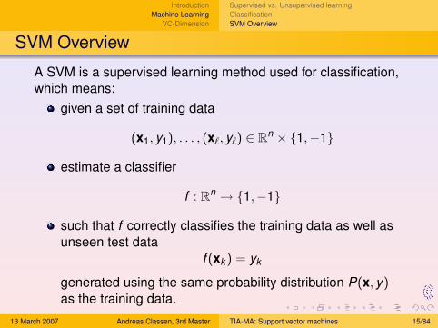
SVM Overview
A SVM is a supervised learning method used for classification,which means:
given a set of training data
(x1, y1), . . . , (x`, y`) ∈ Rn × {1,−1}
estimate a classifier
f : Rn → {1,−1}
such that f correctly classifies the training data as well asunseen test data
f (xk ) = yk
generated using the same probability distribution P(x, y)as the training data.
13 March 2007 Andreas Classen, 3rd Master TIA-MA: Support vector machines 15/84
IntroductionMachine Learning
VC-Dimension
Supervised vs. Unsupervised learningClassificationSVM Overview
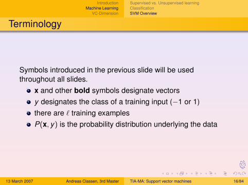
Terminology
Symbols introduced in the previous slide will be usedthroughout all slides.
x and other bold symbols designate vectorsy designates the class of a training input (−1 or 1)there are ` training examplesP(x, y) is the probability distribution underlying the data
13 March 2007 Andreas Classen, 3rd Master TIA-MA: Support vector machines 16/84
IntroductionMachine Learning
VC-Dimension
Risc MinimisationVC-Dimension
Outline
1 Introduction
2 Machine LearningSupervised vs. Unsupervised learningClassificationSVM Overview
3 VC-DimensionRisc MinimisationVC-Dimension
13 March 2007 Andreas Classen, 3rd Master TIA-MA: Support vector machines 17/84
IntroductionMachine Learning
VC-Dimension
Risc MinimisationVC-Dimension
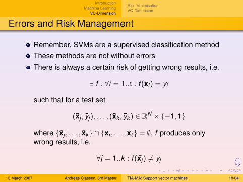
Errors and Risk Management
Remember, SVMs are a supervised classification methodThese methods are not without errorsThere is always a certain risk of getting wrong results, i.e.
∃ f : ∀i = 1..` : f (xi) = yi
such that for a test set
(xj , yj), . . . , (xk , yk ) ∈ RN × {−1, 1}
where {xj , . . . , xk} ∩ {xi , . . . , x`} = ∅, f produces onlywrong results, i.e.
∀j = 1..k : f (xj) 6= yj
13 March 2007 Andreas Classen, 3rd Master TIA-MA: Support vector machines 18/84
IntroductionMachine Learning
VC-Dimension
Risc MinimisationVC-Dimension
Outline
1 Introduction
2 Machine LearningSupervised vs. Unsupervised learningClassificationSVM Overview
3 VC-DimensionRisc MinimisationVC-Dimension
13 March 2007 Andreas Classen, 3rd Master TIA-MA: Support vector machines 19/84
IntroductionMachine Learning
VC-Dimension
Risc MinimisationVC-Dimension
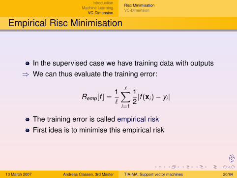
Empirical Risc Minimisation
In the supervised case we have training data with outputs⇒ We can thus evaluate the training error:
Remp[f ] =1`
∑i=1
12|f (xi)− yi |
The training error is called empirical riskFirst idea is to minimise this empirical risk
13 March 2007 Andreas Classen, 3rd Master TIA-MA: Support vector machines 20/84
IntroductionMachine Learning
VC-Dimension
Risc MinimisationVC-Dimension
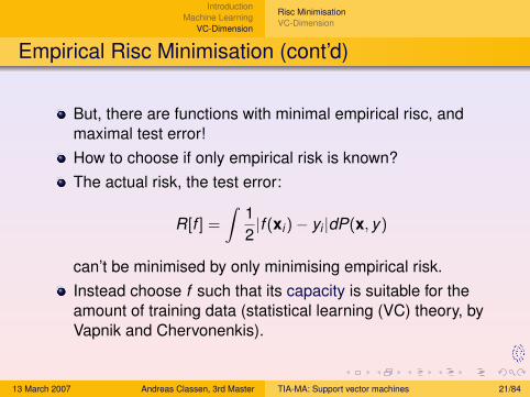
Empirical Risc Minimisation (cont’d)
But, there are functions with minimal empirical risc, andmaximal test error!How to choose if only empirical risk is known?The actual risk, the test error:
R[f ] =
∫12|f (xi)− yi |dP(x, y)
can’t be minimised by only minimising empirical risk.Instead choose f such that its capacity is suitable for theamount of training data (statistical learning (VC) theory, byVapnik and Chervonenkis).
13 March 2007 Andreas Classen, 3rd Master TIA-MA: Support vector machines 21/84
IntroductionMachine Learning
VC-Dimension
Risc MinimisationVC-Dimension
Structural Risc Minimisation
Using capacity concepts, VC theory places bounds on thetest error.
⇒ Minimise these bounds wrt. to capacity and training error⇒ Called structural risc minimisation.
A well known capacity measure is the VC dimension h.
13 March 2007 Andreas Classen, 3rd Master TIA-MA: Support vector machines 22/84
IntroductionMachine Learning
VC-Dimension
Risc MinimisationVC-Dimension
Outline
1 Introduction
2 Machine LearningSupervised vs. Unsupervised learningClassificationSVM Overview
3 VC-DimensionRisc MinimisationVC-Dimension
13 March 2007 Andreas Classen, 3rd Master TIA-MA: Support vector machines 23/84
IntroductionMachine Learning
VC-Dimension
Risc MinimisationVC-Dimension
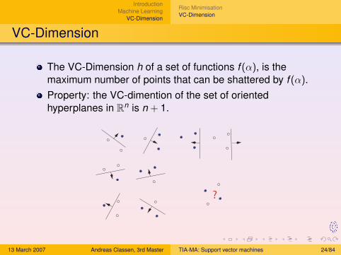
VC-Dimension
The VC-Dimension h of a set of functions f (α), is themaximum number of points that can be shattered by f (α).Property: the VC-dimention of the set of orientedhyperplanes in Rn is n + 1.
?
13 March 2007 Andreas Classen, 3rd Master TIA-MA: Support vector machines 24/84
IntroductionMachine Learning
VC-Dimension
Risc MinimisationVC-Dimension
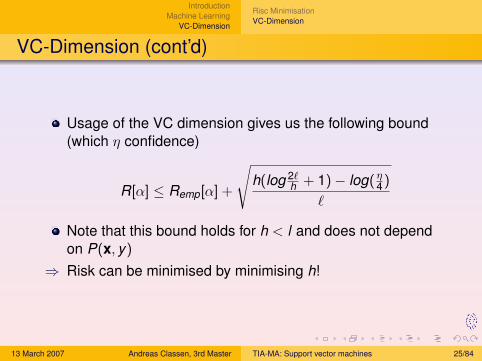
VC-Dimension (cont’d)
Usage of the VC dimension gives us the following bound(which η confidence)
R[α] ≤ Remp[α] +
√h(log 2`
h + 1)− log(η4)
`
Note that this bound holds for h < l and does not dependon P(x, y)
⇒ Risk can be minimised by minimising h!
13 March 2007 Andreas Classen, 3rd Master TIA-MA: Support vector machines 25/84
Linear machines on separable dataLinear machines on nonseparable data
Nonlinear machines on nonseparable data
Part II
Support Vector Machines
13 March 2007 Andreas Classen, 3rd Master TIA-MA: Support vector machines 26/84
Linear machines on separable dataLinear machines on nonseparable data
Nonlinear machines on nonseparable data
Reminder
A SVM is a supervised learning method used for classification:given a set of training data
(x1, y1), . . . , (x`, y`) ∈ RN × {1,−1}
estimate a classifier
f : RN → {1,−1}
such that f correctly classifies the training data as well asunseen data
f (xp) = yp
generated using the same probability distribution P(x, y)as the training data.
13 March 2007 Andreas Classen, 3rd Master TIA-MA: Support vector machines 27/84
Linear machines on separable dataLinear machines on nonseparable data
Nonlinear machines on nonseparable data
Different Situations
There are differnet types of SV machines, based on theproperties of the training set.
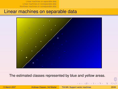
1 Linear machines on separable dataBoth classes form disjoint convex setsNo training errorEasiest case
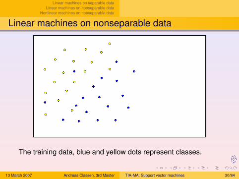
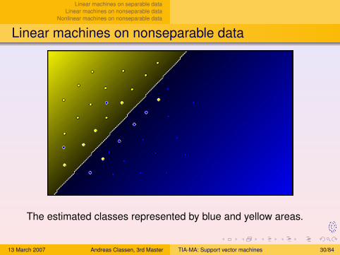
2 Linear machines on nonseparable dataGeneralisation of the previous caseBoth classes overlay at some pointThere will thus be training error
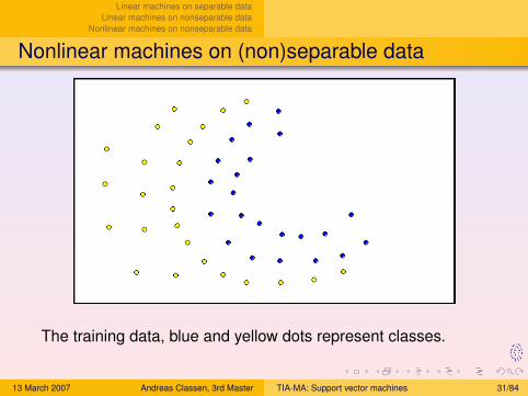
3 Nonlinear machines on nonseparable dataGeneralisation of both previous casesBoth classes are only separable with a non-linear function
13 March 2007 Andreas Classen, 3rd Master TIA-MA: Support vector machines 28/84
Linear machines on separable dataLinear machines on nonseparable data
Nonlinear machines on nonseparable data
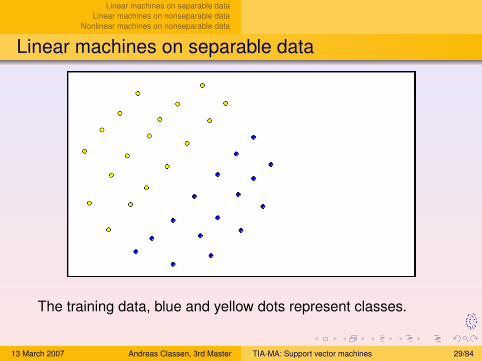
Linear machines on separable data
The training data, blue and yellow dots represent classes.
13 March 2007 Andreas Classen, 3rd Master TIA-MA: Support vector machines 29/84
Linear machines on separable dataLinear machines on nonseparable data
Nonlinear machines on nonseparable data
Linear machines on separable data
The estimated classes represented by blue and yellow areas.
13 March 2007 Andreas Classen, 3rd Master TIA-MA: Support vector machines 29/84
Linear machines on separable dataLinear machines on nonseparable data
Nonlinear machines on nonseparable data
Linear machines on nonseparable data
The training data, blue and yellow dots represent classes.
13 March 2007 Andreas Classen, 3rd Master TIA-MA: Support vector machines 30/84
Linear machines on separable dataLinear machines on nonseparable data
Nonlinear machines on nonseparable data
Linear machines on nonseparable data
The estimated classes represented by blue and yellow areas.
13 March 2007 Andreas Classen, 3rd Master TIA-MA: Support vector machines 30/84
Linear machines on separable dataLinear machines on nonseparable data
Nonlinear machines on nonseparable data
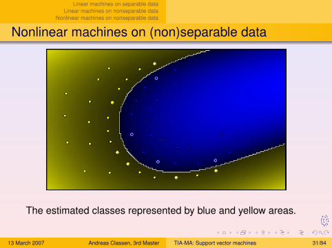
Nonlinear machines on (non)separable data
The training data, blue and yellow dots represent classes.
13 March 2007 Andreas Classen, 3rd Master TIA-MA: Support vector machines 31/84
Linear machines on separable dataLinear machines on nonseparable data
Nonlinear machines on nonseparable data
Nonlinear machines on (non)separable data
The estimated classes represented by blue and yellow areas.
13 March 2007 Andreas Classen, 3rd Master TIA-MA: Support vector machines 31/84
Linear machines on separable dataLinear machines on nonseparable data
Nonlinear machines on nonseparable data
SituationOptimisation problem
Outline
4 Linear machines on separable dataSituationOptimisation problem
5 Linear machines on nonseparable dataSituationOptimisation problem
6 Nonlinear machines on nonseparable dataThe Kernel TrickExample
13 March 2007 Andreas Classen, 3rd Master TIA-MA: Support vector machines 32/84
Linear machines on separable dataLinear machines on nonseparable data
Nonlinear machines on nonseparable data
SituationOptimisation problem
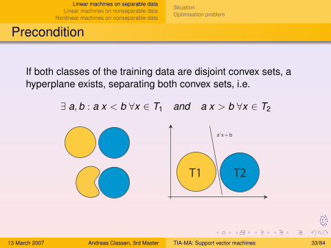
Precondition
If both classes of the training data are disjoint convex sets, ahyperplane exists, separating both convex sets, i.e.
∃ a, b : a x < b ∀x ∈ T1 and a x > b ∀x ∈ T2
a’ x = b
T1 T2
13 March 2007 Andreas Classen, 3rd Master TIA-MA: Support vector machines 33/84
Linear machines on separable dataLinear machines on nonseparable data
Nonlinear machines on nonseparable data
SituationOptimisation problem
Outline
4 Linear machines on separable dataSituationOptimisation problem
5 Linear machines on nonseparable dataSituationOptimisation problem
6 Nonlinear machines on nonseparable dataThe Kernel TrickExample
13 March 2007 Andreas Classen, 3rd Master TIA-MA: Support vector machines 34/84
Linear machines on separable dataLinear machines on nonseparable data
Nonlinear machines on nonseparable data
SituationOptimisation problem
Situation
w
{x | (w x) + b = 0}.
x2
x1
yi = −1
yi = +1❍
❍
❍❍
◆
◆
◆
◆
❍
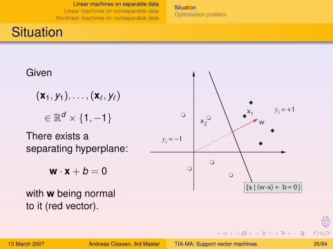
Given
(x1, y1), . . . , (x`, y`)
∈ Rd × {1,−1}
There exists aseparating hyperplane:
w · x + b = 0
with w being normalto it (red vector).
13 March 2007 Andreas Classen, 3rd Master TIA-MA: Support vector machines 35/84
Linear machines on separable dataLinear machines on nonseparable data
Nonlinear machines on nonseparable data
SituationOptimisation problem
Situation (cont’d)
w
{x | (w x) + b = 0}.
}{x | (w x) + b = −1}. {x | (w x) + b = +1}.
x2
x1
yi = −1
yi = +1❍
❍
❍❍
◆
◆
◆
◆
❍
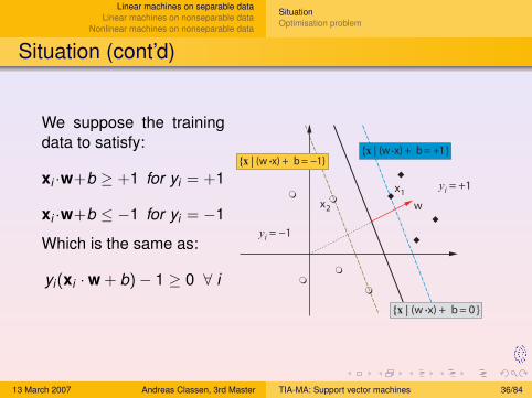
We suppose the trainingdata to satisfy:
xi ·w+b ≥ +1 for yi = +1
xi ·w+b ≤ −1 for yi = −1
Which is the same as:
yi(xi ·w + b)− 1 ≥ 0 ∀ i
13 March 2007 Andreas Classen, 3rd Master TIA-MA: Support vector machines 36/84
Linear machines on separable dataLinear machines on nonseparable data
Nonlinear machines on nonseparable data
SituationOptimisation problem
Situation (cont’d)
w
{x | (w x) + b = 0}.
}{x | (w x) + b = −1}. {x | (w x) + b = +1}.
x2
x1
yi = −1
yi = +1❍
❍
❍❍
◆
◆
◆
◆
❍
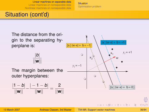
The distance from the ori-gin to the separating hy-perplane is:
|b|||w||
The margin between theouter hyperplanes:
|1− b|||w||
−| − 1− b|||w||
=2||w||
13 March 2007 Andreas Classen, 3rd Master TIA-MA: Support vector machines 36/84
Linear machines on separable dataLinear machines on nonseparable data
Nonlinear machines on nonseparable data
SituationOptimisation problem
Situation (cont’d)
w
{x | (w x) + b = 0}.
}{x | (w x) + b = −1}. {x | (w x) + b = +1}.
x2
x1
yi = −1
yi = +1❍
❍
❍❍
◆
◆
◆
◆
❍
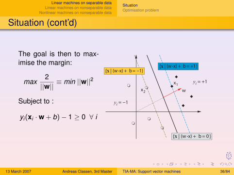
The goal is then to max-imise the margin:
max2||w||
≡ min ||w||2
Subject to :
yi(xi ·w + b)− 1 ≥ 0 ∀ i
13 March 2007 Andreas Classen, 3rd Master TIA-MA: Support vector machines 36/84
Linear machines on separable dataLinear machines on nonseparable data
Nonlinear machines on nonseparable data
SituationOptimisation problem
Outline
4 Linear machines on separable dataSituationOptimisation problem
5 Linear machines on nonseparable dataSituationOptimisation problem
6 Nonlinear machines on nonseparable dataThe Kernel TrickExample
13 March 2007 Andreas Classen, 3rd Master TIA-MA: Support vector machines 37/84
Linear machines on separable dataLinear machines on nonseparable data
Nonlinear machines on nonseparable data
SituationOptimisation problem
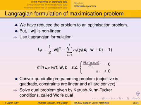
Langragian formulation of maximisation problem
We have reduced the problem to an optimisation problem.But, ||w|| is non-linear
⇒ Use Lagrangian formulation
LP ≡12||w||2 −
∑i=1
αi(yi(xi ·w + b)− 1)
min LP wrt . w, b s.c.
{∂LP(w,b,α)
∂αi= 0
αi ≥ 0
Convex quadratic programming problem (objective isquadratic, constraints are linear and all are convex)
⇒ Solve dual problem given by Karush-Kuhn-Tuckerconditions, called Wolfe dual
13 March 2007 Andreas Classen, 3rd Master TIA-MA: Support vector machines 38/84
Linear machines on separable dataLinear machines on nonseparable data
Nonlinear machines on nonseparable data
SituationOptimisation problem
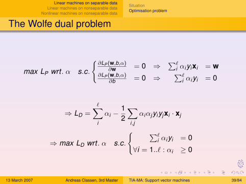
The Wolfe dual problem
max LP wrt . α s.c.
{∂LP(w,b,α)
∂w = 0 ⇒∑`
i αiyixi = w∂LP(w,b,α)
∂b = 0 ⇒∑`
i αiyi = 0
⇒ LD =∑
i
αi −12
∑i,j
αiαjyiyjxi · xj
⇒ max LD wrt . α s.c.
{ ∑`i αiyi = 0
∀i = 1..` : αi ≥ 0
13 March 2007 Andreas Classen, 3rd Master TIA-MA: Support vector machines 39/84
Linear machines on separable dataLinear machines on nonseparable data
Nonlinear machines on nonseparable data
SituationOptimisation problem
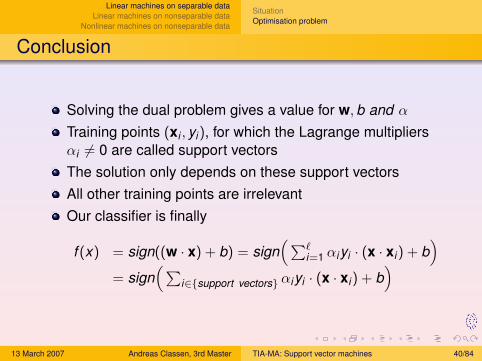
Conclusion
Solving the dual problem gives a value for w, b and α
Training points (xi , yi), for which the Lagrange multipliersαi 6= 0 are called support vectorsThe solution only depends on these support vectorsAll other training points are irrelevantOur classifier is finally
f (x) = sign((w · x) + b) = sign(∑`
i=1 αiyi · (x · xi) + b)
= sign(∑
i∈{support vectors} αiyi · (x · xi) + b)
13 March 2007 Andreas Classen, 3rd Master TIA-MA: Support vector machines 40/84
Linear machines on separable dataLinear machines on nonseparable data
Nonlinear machines on nonseparable data
SituationOptimisation problem
Outline
4 Linear machines on separable dataSituationOptimisation problem
5 Linear machines on nonseparable dataSituationOptimisation problem
6 Nonlinear machines on nonseparable dataThe Kernel TrickExample
13 March 2007 Andreas Classen, 3rd Master TIA-MA: Support vector machines 41/84
Linear machines on separable dataLinear machines on nonseparable data
Nonlinear machines on nonseparable data
SituationOptimisation problem
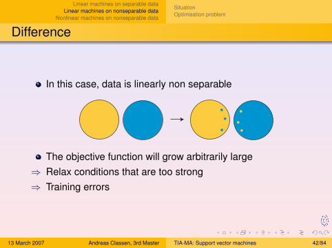
Difference
In this case, data is linearly non separable
The objective function will grow arbitrarily large⇒ Relax conditions that are too strong⇒ Training errors
13 March 2007 Andreas Classen, 3rd Master TIA-MA: Support vector machines 42/84
Linear machines on separable dataLinear machines on nonseparable data
Nonlinear machines on nonseparable data
SituationOptimisation problem
Outline
4 Linear machines on separable dataSituationOptimisation problem
5 Linear machines on nonseparable dataSituationOptimisation problem
6 Nonlinear machines on nonseparable dataThe Kernel TrickExample
13 March 2007 Andreas Classen, 3rd Master TIA-MA: Support vector machines 43/84
Linear machines on separable dataLinear machines on nonseparable data
Nonlinear machines on nonseparable data
SituationOptimisation problem
Situation
w
{x | (w x) + b = 0}.
}{x | (w x) + b = −1}.{x | (w x) + b = +1}.
x2
x1
yi = −1
yi = +1❍
❍❍
◆
◆
◆
◆
❍
◆ −ξ||w||
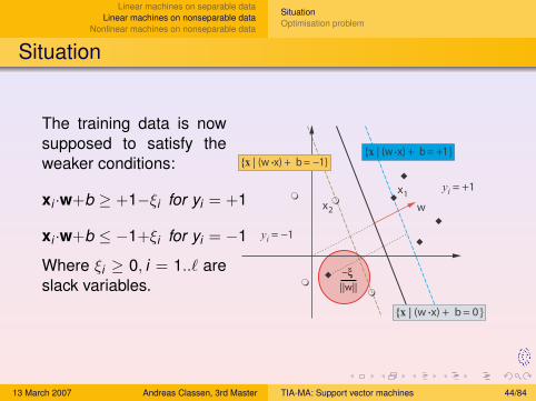
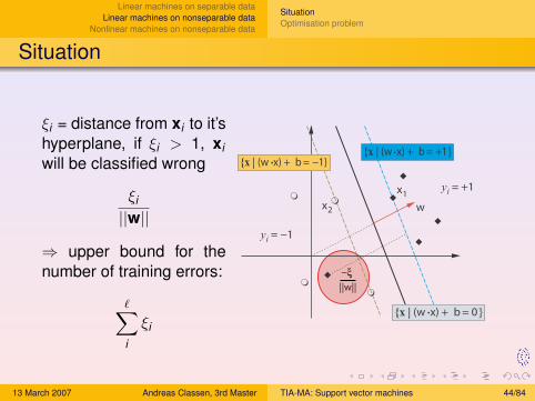
The training data is nowsupposed to satisfy theweaker conditions:
xi ·w+b ≥ +1−ξi for yi = +1
xi ·w+b ≤ −1+ξi for yi = −1
Where ξi ≥ 0, i = 1..` areslack variables.
13 March 2007 Andreas Classen, 3rd Master TIA-MA: Support vector machines 44/84
Linear machines on separable dataLinear machines on nonseparable data
Nonlinear machines on nonseparable data
SituationOptimisation problem
Situation
w
{x | (w x) + b = 0}.
}{x | (w x) + b = −1}.{x | (w x) + b = +1}.
x2
x1
yi = −1
yi = +1❍
❍❍
◆
◆
◆
◆
❍
◆ −ξ||w||
ξi = distance from xi to it’shyperplane, if ξi > 1, xiwill be classified wrong
ξi
||w||
⇒ upper bound for thenumber of training errors:
∑i
ξi
13 March 2007 Andreas Classen, 3rd Master TIA-MA: Support vector machines 44/84
Linear machines on separable dataLinear machines on nonseparable data
Nonlinear machines on nonseparable data
SituationOptimisation problem
Situation
w
{x | (w x) + b = 0}.
}{x | (w x) + b = −1}.{x | (w x) + b = +1}.
x2
x1
yi = −1
yi = +1❍
❍❍
◆
◆
◆
◆
❍
◆ −ξ||w||
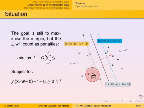
The goal is still to max-imise the margin, but theξi will count as penalties:
min ||w||2 + C∑i=1
ξi
Subject to :
yi(xi ·w+b)−1+ξi ≥ 0 ∀ i
13 March 2007 Andreas Classen, 3rd Master TIA-MA: Support vector machines 44/84
Linear machines on separable dataLinear machines on nonseparable data
Nonlinear machines on nonseparable data
SituationOptimisation problem
Outline
4 Linear machines on separable dataSituationOptimisation problem
5 Linear machines on nonseparable dataSituationOptimisation problem
6 Nonlinear machines on nonseparable dataThe Kernel TrickExample
13 March 2007 Andreas Classen, 3rd Master TIA-MA: Support vector machines 45/84
Linear machines on separable dataLinear machines on nonseparable data
Nonlinear machines on nonseparable data
SituationOptimisation problem
Langragian formulation of maximisation problem
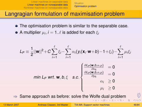
The optimisation problem is similar to the separable case.A multiplier µi , i = 1..` is added for each ξi
LP ≡12||w||2+C
∑i=1
ξi−∑i=1
αi(yi(xi ·w+b)−1+ξi)−∑i=1
µiξi
min LP wrt . w, b, ξ s.c.
∂LP(w,b,α,µ)∂αi
= 0∂LP(w,b,α,µ)
∂µi= 0
αi ≥ 0
µi ≥ 0
⇒ Same approach as before: solve the Wolfe dual problem
13 March 2007 Andreas Classen, 3rd Master TIA-MA: Support vector machines 46/84
Linear machines on separable dataLinear machines on nonseparable data
Nonlinear machines on nonseparable data
SituationOptimisation problem
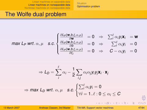
The Wolfe dual problem
max LP wrt . α, µ s.c.
∂LP(w,b,ξ,α,µ)
∂w = 0 ⇒∑`
i αiyixi = w∂LP(w,b,ξ,α,µ)
∂b = 0 ⇒∑`
i αiyi = 0∂LP(w,b,ξ,α,µ)
∂ξi= 0 ⇒ C − αiyi = 0
⇒ LD =∑
i
αi −12
∑i,j
αiαjyiyjxi · xj
⇒ max LD wrt . α, µ s.c.
{∑`i αiyi = 0
∀i = 1..` : 0 ≤ αi ≤ C
13 March 2007 Andreas Classen, 3rd Master TIA-MA: Support vector machines 47/84
Linear machines on separable dataLinear machines on nonseparable data
Nonlinear machines on nonseparable data
SituationOptimisation problem
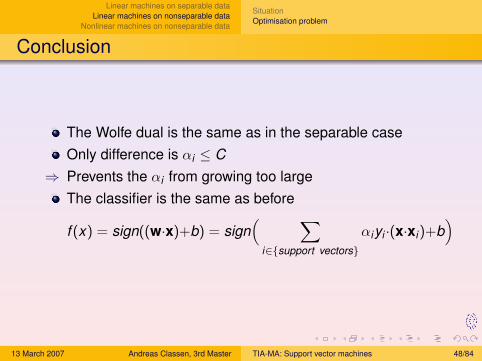
Conclusion
The Wolfe dual is the same as in the separable caseOnly difference is αi ≤ C
⇒ Prevents the αi from growing too largeThe classifier is the same as before
f (x) = sign((w·x)+b) = sign( ∑
i∈{support vectors}
αiyi ·(x·xi)+b)
13 March 2007 Andreas Classen, 3rd Master TIA-MA: Support vector machines 48/84
Linear machines on separable dataLinear machines on nonseparable data
Nonlinear machines on nonseparable data
The Kernel TrickExample
Outline
4 Linear machines on separable dataSituationOptimisation problem
5 Linear machines on nonseparable dataSituationOptimisation problem
6 Nonlinear machines on nonseparable dataThe Kernel TrickExample
13 March 2007 Andreas Classen, 3rd Master TIA-MA: Support vector machines 49/84
Linear machines on separable dataLinear machines on nonseparable data
Nonlinear machines on nonseparable data
The Kernel TrickExample
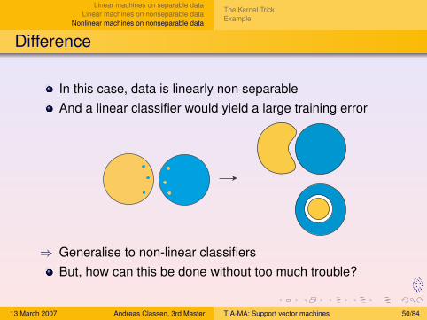
Difference
In this case, data is linearly non separableAnd a linear classifier would yield a large training error
⇒ Generalise to non-linear classifiersBut, how can this be done without too much trouble?
13 March 2007 Andreas Classen, 3rd Master TIA-MA: Support vector machines 50/84
Linear machines on separable dataLinear machines on nonseparable data
Nonlinear machines on nonseparable data
The Kernel TrickExample
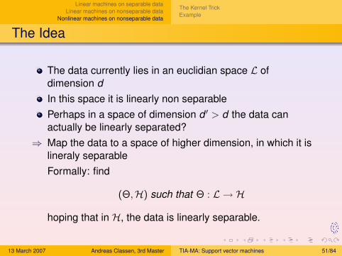
The Idea
The data currently lies in an euclidian space L ofdimension dIn this space it is linearly non separablePerhaps in a space of dimension d ′ > d the data canactually be linearly separated?
⇒ Map the data to a space of higher dimension, in which it islineraly separableFormally: find
(Θ,H) such that Θ : L → H
hoping that in H, the data is linearly separable.
13 March 2007 Andreas Classen, 3rd Master TIA-MA: Support vector machines 51/84
Linear machines on separable dataLinear machines on nonseparable data
Nonlinear machines on nonseparable data
The Kernel TrickExample
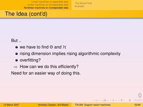
The Idea (cont’d)
But ..we have to find Θ and Hrising dimension implies rising algorithmic complexityoverfitting?
⇒ How can we do this efficiently?Need for an easier way of doing this.
13 March 2007 Andreas Classen, 3rd Master TIA-MA: Support vector machines 52/84
Linear machines on separable dataLinear machines on nonseparable data
Nonlinear machines on nonseparable data
The Kernel TrickExample
Outline
4 Linear machines on separable dataSituationOptimisation problem
5 Linear machines on nonseparable dataSituationOptimisation problem
6 Nonlinear machines on nonseparable dataThe Kernel TrickExample
13 March 2007 Andreas Classen, 3rd Master TIA-MA: Support vector machines 53/84
Linear machines on separable dataLinear machines on nonseparable data
Nonlinear machines on nonseparable data
The Kernel TrickExample
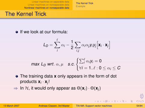
The Kernel Trick
If we look at our formula:
LD =∑
i
αi −12
∑i,j
αiαjyiyj
[xi · xj
]
max LD wrt . α, µ s.c.
{∑`i αiyi = 0
∀i = 1..` : 0 ≤ αi ≤ C
The training data x only appears in the form of dotproducts xi · xj !
⇒ In H, it would only appear as Θ(xi) ·Θ(xj)
13 March 2007 Andreas Classen, 3rd Master TIA-MA: Support vector machines 54/84
Linear machines on separable dataLinear machines on nonseparable data
Nonlinear machines on nonseparable data
The Kernel TrickExample
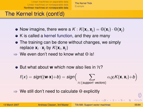
The Kernel trick (cont’d)
Now imagine, there were a K : K (xi , xj) = Θ(xi) ·Θ(xj)
K is called a kernel function, and they are manyThe training can be done without changes, we simplyreplace xi · xj by K (xi , xj)
⇒ We even don’t need to know what Θ is!
But what about w which now also lies in H?
f (x) = sign((w·x)+b) = sign( ∑
i∈{support vectors}
αiyiK (x, xi)+b)
⇒ We still don’t need to calculate Θ explicitly
13 March 2007 Andreas Classen, 3rd Master TIA-MA: Support vector machines 55/84
Linear machines on separable dataLinear machines on nonseparable data
Nonlinear machines on nonseparable data
The Kernel TrickExample
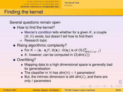
Finding the kernel
Several questions remain openHow to find the kernel?
Mercer’s condition tells whether for a given K , a couple(Θ,H) exists, but doesn’t tell how to find them
⇒ Research topicRising algorithmic complexity?
For K = (xi · xj)p, Θ(xi) ·Θ(xj) is of O(Cp
dim(L)+p−1)
K , however, can be computed in O(dim(L))
Overfitting?Mapping data to a high dimensional space is generally badfor generalisationThe classifier in H has dim(H) + 1 parameters!But, the intrinsic dimension is still dim(L), and there areonly ` parameters
13 March 2007 Andreas Classen, 3rd Master TIA-MA: Support vector machines 56/84
Linear machines on separable dataLinear machines on nonseparable data
Nonlinear machines on nonseparable data
The Kernel TrickExample
Outline
4 Linear machines on separable dataSituationOptimisation problem
5 Linear machines on nonseparable dataSituationOptimisation problem
6 Nonlinear machines on nonseparable dataThe Kernel TrickExample
13 March 2007 Andreas Classen, 3rd Master TIA-MA: Support vector machines 57/84
Linear machines on separable dataLinear machines on nonseparable data
Nonlinear machines on nonseparable data
The Kernel TrickExample
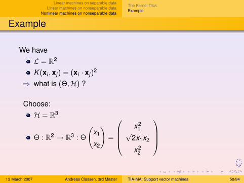
Example
We haveL = R2
K (xi , xj) = (xi · xj)2
⇒ what is (Θ,H) ?
Choose:H = R3
Θ : R2 → R3 : Θ
(x1
x2
)=
x2
1√2x1x2
x22
13 March 2007 Andreas Classen, 3rd Master TIA-MA: Support vector machines 58/84
Linear machines on separable dataLinear machines on nonseparable data
Nonlinear machines on nonseparable data
The Kernel TrickExample
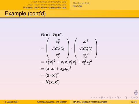
Example (cont’d)
Θ(x) ·Θ(x′)
=
x2
1√2x1x2
x22
·
x ′1
2√
2x ′1x ′2x ′2
2
= x2
1 x ′12 + x1x2x ′1x ′2 + x2
2 x ′22
= (x1x ′1 + x2x ′2)2
= (x · x′)2
= K (x, x′)
13 March 2007 Andreas Classen, 3rd Master TIA-MA: Support vector machines 59/84
Linear machines on separable dataLinear machines on nonseparable data
Nonlinear machines on nonseparable data
The Kernel TrickExample
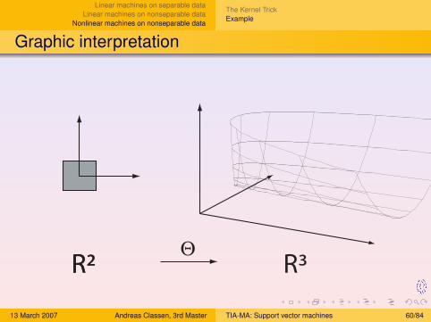
Graphic interpretation
R²R² R³Θ
13 March 2007 Andreas Classen, 3rd Master TIA-MA: Support vector machines 60/84
Linear machines on separable dataLinear machines on nonseparable data
Nonlinear machines on nonseparable data
The Kernel TrickExample
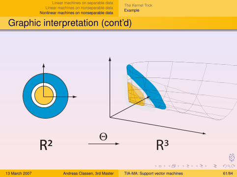
Graphic interpretation (cont’d)
R²R² R³Θ
13 March 2007 Andreas Classen, 3rd Master TIA-MA: Support vector machines 61/84
Linear machines on separable dataLinear machines on nonseparable data
Nonlinear machines on nonseparable data
The Kernel TrickExample
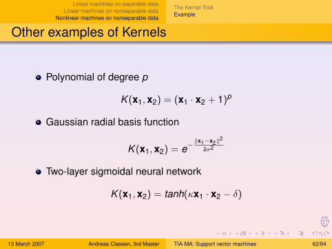
Other examples of Kernels
Polynomial of degree p
K (x1, x2) = (x1 · x2 + 1)p
Gaussian radial basis function
K (x1, x2) = e−‖x1−x2‖
2
2σ2
Two-layer sigmoidal neural network
K (x1, x2) = tanh(κx1 · x2 − δ)
13 March 2007 Andreas Classen, 3rd Master TIA-MA: Support vector machines 62/84
Complexity resultsFace Recognition Illustration
References
Part III
Conclusion
13 March 2007 Andreas Classen, 3rd Master TIA-MA: Support vector machines 63/84
Complexity resultsFace Recognition Illustration
References
Outline
7 Complexity results
8 Face Recognition IllustrationSystemConclusion
9 References
13 March 2007 Andreas Classen, 3rd Master TIA-MA: Support vector machines 64/84
Complexity resultsFace Recognition Illustration
References
Solving SVMs
Training a SVM means solving the optimisation problemSolving analytically is rarely possible
⇒ In real world, the problem has to be solved numericallyExisting tools for solving lineraly constrained convexquadratic problems can be reusedLarge problems, however, require their own solutionstrategy
⇒ Training complexity depends on the choosen solutionmethod
13 March 2007 Andreas Classen, 3rd Master TIA-MA: Support vector machines 65/84
Complexity resultsFace Recognition Illustration
References
Advantage of kernels
As seen before, even in high-dimensional spaces, kernelfunctions reduce complexity dramaticallyConstructing hyperplanes in high-dimensional spaces isdone with a reasonable amount of computing
In the following:
d = dim(L)
Ns =number of support vectors` =number of training samples
13 March 2007 Andreas Classen, 3rd Master TIA-MA: Support vector machines 66/84
Complexity resultsFace Recognition Illustration
References
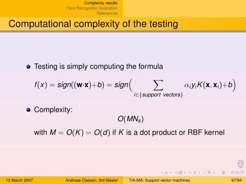
Computational complexity of the testing
Testing is simply computing the formula
f (x) = sign((w·x)+b) = sign( ∑
i∈{support vectors}
αiyiK (x, xi)+b)
Complexity:O(MNs)
with M = O(K ) = O(d) if K is a dot product or RBF kernel
13 March 2007 Andreas Classen, 3rd Master TIA-MA: Support vector machines 67/84
Complexity resultsFace Recognition Illustration
References
SystemConclusion
Outline
7 Complexity results
8 Face Recognition IllustrationSystemConclusion
9 References
13 March 2007 Andreas Classen, 3rd Master TIA-MA: Support vector machines 68/84
Complexity resultsFace Recognition Illustration
References
SystemConclusion
The problem
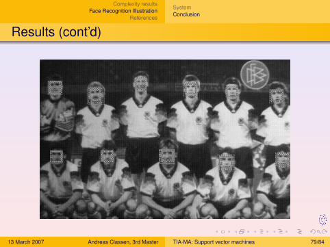
Taken from [Osuna1997]Input: an imageOutput: the coordinates of faces found in this image
Difficult problem, important pattern variationsfacial appearence differspresence of other objects like glasses, moustacheslight source and resulting shadows
13 March 2007 Andreas Classen, 3rd Master TIA-MA: Support vector machines 69/84
Complexity resultsFace Recognition Illustration
References
SystemConclusion
Approach
Problem devided into two tasks1 Find all possible face-like details of the image
Scan the image exhaustively⇒ Identify every sub-image for every considered scale
2 Classify these details into face and non-faceTrain a SV machine for face detectionClassify each sub-image with this machine
13 March 2007 Andreas Classen, 3rd Master TIA-MA: Support vector machines 70/84
Complexity resultsFace Recognition Illustration
References
SystemConclusion
Outline
7 Complexity results
8 Face Recognition IllustrationSystemConclusion
9 References
13 March 2007 Andreas Classen, 3rd Master TIA-MA: Support vector machines 71/84
Complexity resultsFace Recognition Illustration
References
SystemConclusion
Training
Training based on a database of face and non-face 19× 19pixel imagesThe kernel is 2nd degree polynomialPreprocessing of the image is performed
Masking: reduce the pixels from 19× 19 = 361 to 283, inorder to reduce noiseIllumination correction: reduce light and heavy shadowsHistogram equalisation: compensate for differences incameras
Extend training by bootstrapping, i.e. testing errors of atrained machine are stored and used as negativeexamples in the next training
13 March 2007 Andreas Classen, 3rd Master TIA-MA: Support vector machines 72/84
Complexity resultsFace Recognition Illustration
References
SystemConclusion
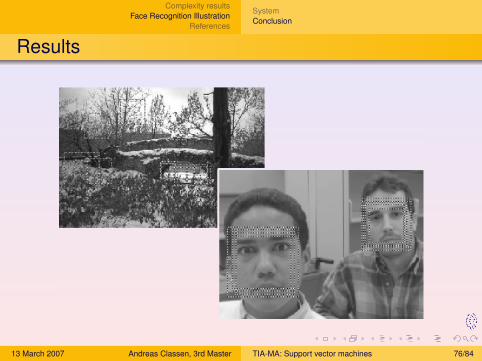
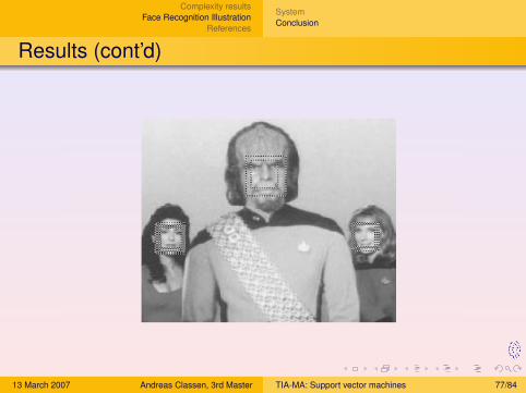
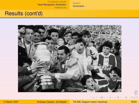
Testing
Re-scale the image, to get different scales of facesCut the 19× 19 windowsFor each one
Apply the preprocessing as in the trainingClassify the sub-imagesIf positive, indicate the position of the face on the originalimage
13 March 2007 Andreas Classen, 3rd Master TIA-MA: Support vector machines 73/84
Complexity resultsFace Recognition Illustration
References
SystemConclusion
Outline
7 Complexity results
8 Face Recognition IllustrationSystemConclusion
9 References
13 March 2007 Andreas Classen, 3rd Master TIA-MA: Support vector machines 74/84
Complexity resultsFace Recognition Illustration
References
SystemConclusion
Conclusion
Developing an intelligent system using SVMs is wellbeyond applying the mathematical formulaeTraining examples have to be collected carefullyRaw data generally doesn’t work, some preprocessing hasto be done
13 March 2007 Andreas Classen, 3rd Master TIA-MA: Support vector machines 75/84
Complexity resultsFace Recognition Illustration
References
SystemConclusion
Results
13 March 2007 Andreas Classen, 3rd Master TIA-MA: Support vector machines 76/84
Complexity resultsFace Recognition Illustration
References
SystemConclusion
Results (cont’d)
13 March 2007 Andreas Classen, 3rd Master TIA-MA: Support vector machines 77/84
Complexity resultsFace Recognition Illustration
References
SystemConclusion
Results (cont’d)
13 March 2007 Andreas Classen, 3rd Master TIA-MA: Support vector machines 78/84
Complexity resultsFace Recognition Illustration
References
SystemConclusion
Results (cont’d)
13 March 2007 Andreas Classen, 3rd Master TIA-MA: Support vector machines 79/84
Complexity resultsFace Recognition Illustration
References
Outline
7 Complexity results
8 Face Recognition IllustrationSystemConclusion
9 References
13 March 2007 Andreas Classen, 3rd Master TIA-MA: Support vector machines 80/84
Complexity resultsFace Recognition Illustration
References
References I
C. J. C. Burges.A tutorial on support vector machines for pattern recognition.Data Min. Knowl. Discov., 2(2):121–167, 1998.L. Kaufman.Solving the quadratic programming problem arising in supportvector classification.pages 147–167, 1999.R. S. Ledley and C. Suen, editors.Pattern Recognition Journal.Elsevier, 2007.E. Osuna, R. Freund, and F. Girosi.Support vector machines: Training and applications.Technical Report AIM-1602, Massachusetts Institute ofTechnology, 1997.
13 March 2007 Andreas Classen, 3rd Master TIA-MA: Support vector machines 81/84
Complexity resultsFace Recognition Illustration
References
References II
F. Provost, editor.Machine Learning Journal.Springer, 2007.C. C. Rodriguez.The kernel trick.Technical report, University at Albany, 2004.B. Schölkopf, C. Burges, and A. J. Smola.Advances in Kernel Methods - Support Vector Learning.MIT Press, Cambridge, MA, 1999.
13 March 2007 Andreas Classen, 3rd Master TIA-MA: Support vector machines 82/84
Summary
Support vector machines are trained classifiersThey are based in VC-theory and implement structural riskminimisationAlthough they only classify into classes 1 and −1 they caneasily be extended to classify an arbitrary number ofclassesThey have a good generalisation performanceChoice of the Kernel is trickyEven with high-dimensional kernels, computationalcomplexity is reasonableLarge area of applications
13 March 2007 Andreas Classen, 3rd Master TIA-MA: Support vector machines 83/84
The End - Thank you for your attention.
13 March 2007 Andreas Classen, 3rd Master TIA-MA: Support vector machines 84/84