TECHNIQUES BASED ON CONCEPTS OF IMPEDANCE

Ch. 10

TECHNIQUES BASED

ON CONCEPTS OF

IMPEDANCE

10.1 INTRODUCTION

In previous chapters we have discussed ways of studying electrode reactions through

large perturbations on the system.

By imposing potential sweeps, potential steps, or current steps, we typically drive the

electrode to a condition far from equilibrium.

we observe the response, which is usually a transient signal.

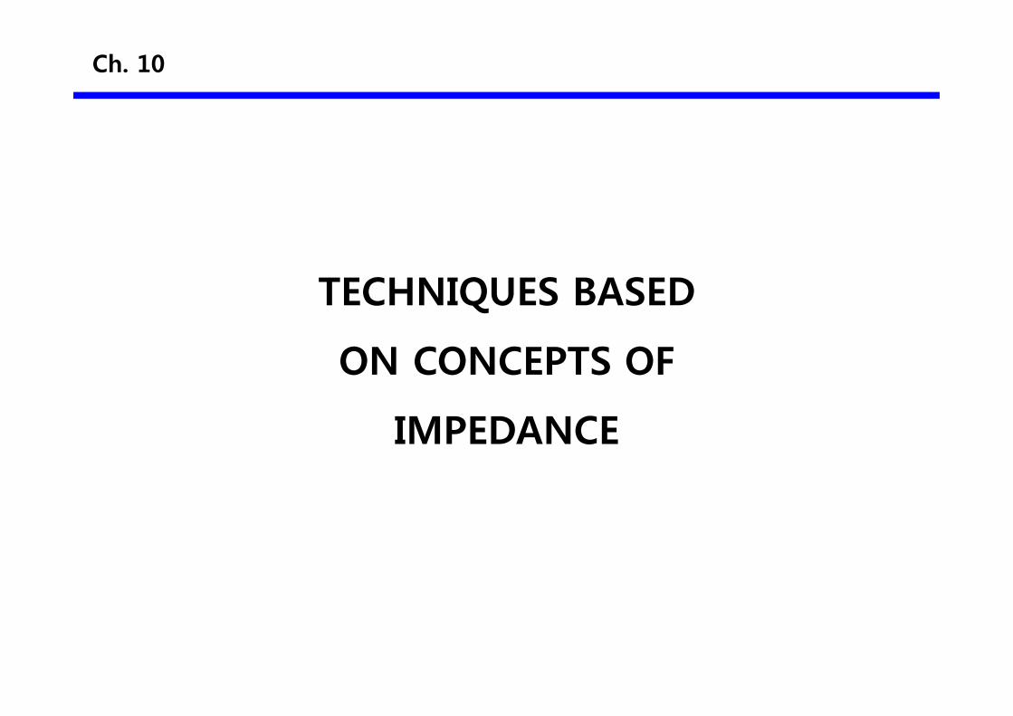
Another approach is to perturb the cell with an alternating signal of small magnitude

and to observe the way in which the system follows the perturbation at steady state.

10.1 INTRODUCTION

Many advantages

(a) an experimental ability to make high-precision measurements because the response

may be indefinitely steady and can therefore be averaged over a long term,

(b) an ability to treat the response theoretically by linearized (or otherwise simplified)

current-potential characteristics,

(c) measurement over a wide time (or frequency) range (104 to 10-6 s or 10-4 to 106 Hz).

Since one usually works close to equilibrium,

one often does not require detailed knowledge about the behavior of the i-E

response curve over great ranges of overpotential.

This advantage leads to important simplifications in treating kinetics and diffusion.

10.1 INTRODUCTION

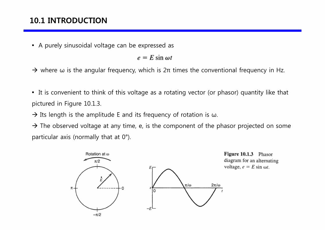
A purely sinusoidal voltage can be expressed as

where ω is the angular frequency, which is 2π times the conventional frequency in Hz.

It is convenient to think of this voltage as a rotating vector (or phasor) quantity like that

pictured in Figure 10.1.3.

Its length is the amplitude E and its frequency of rotation is ω.

The observed voltage at any time, e, is the component of the phasor projected on some

particular axis (normally that at 0°).

10.1 INTRODUCTION

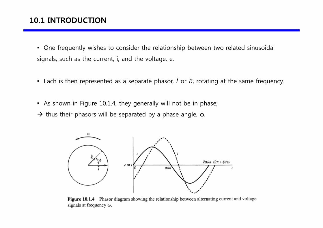
One frequently wishes to consider the relationship between two related sinusoidal

signals, such as the current, i, and the voltage, e.

Each is then represented as a separate phasor, or , rotating at the same frequency.

As shown in Figure 10.1.4, they generally will not be in phase;

thus their phasors will be separated by a phase angle, ф.

10.1 INTRODUCTION

One of the phasors, usually , is taken as a reference signal, and ф is measured with

respect to it.

In the figure, the current lags the voltage. It can be expressed generally as

The relationship between two phasors at the same frequency remains constant as

they rotate

hence the phase angle is constant.

10.1 INTRODUCTION

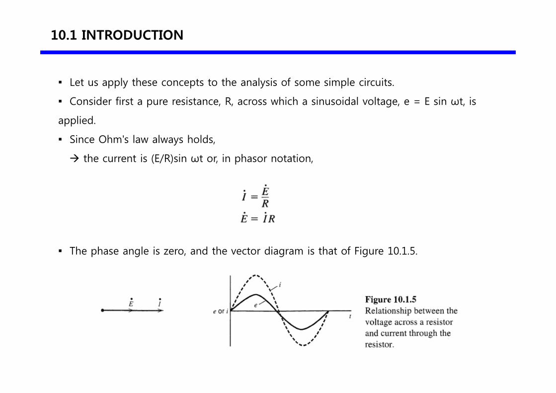
Let us apply these concepts to the analysis of some simple circuits.

Consider first a pure resistance, R, across which a sinusoidal voltage, e = E sin ωt, is

applied.

Since Ohm's law always holds,

the current is (E/R)sin ωt or, in phasor notation,

The phase angle is zero, and the vector diagram is that of Figure 10.1.5.

10.1 INTRODUCTION

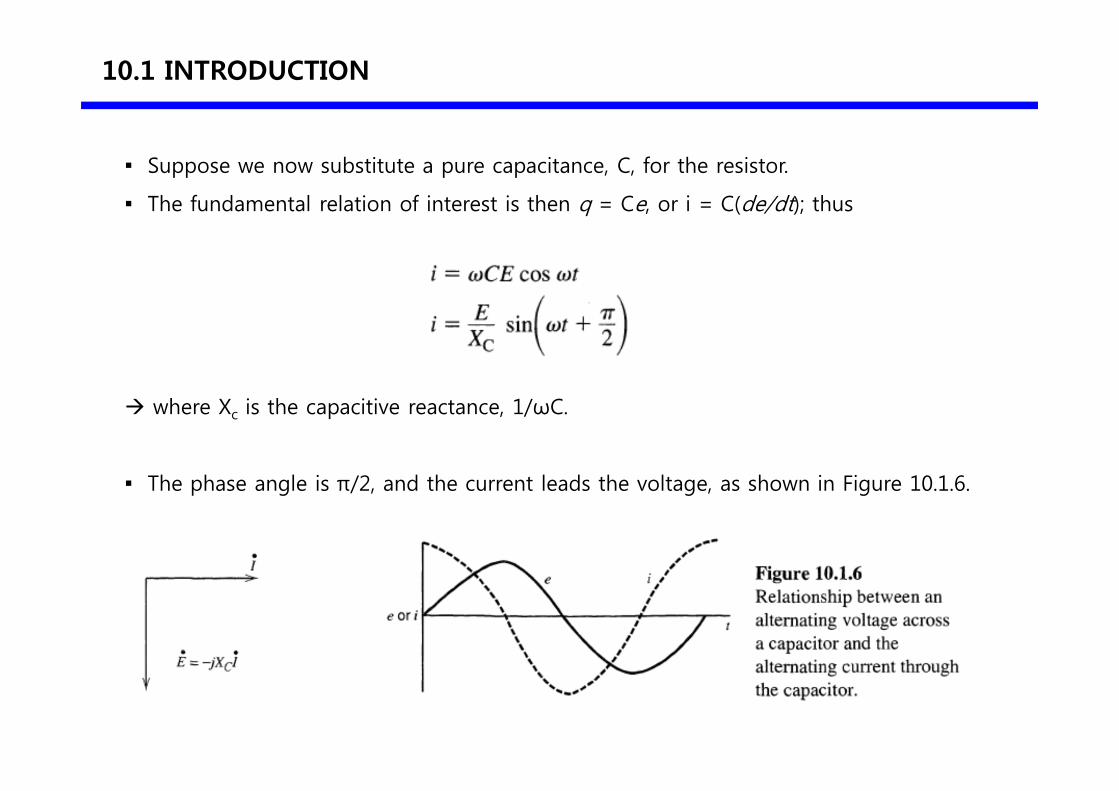
Suppose we now substitute a pure capacitance, C, for the resistor.

The fundamental relation of interest is then q = Ce, or i = C(de/dt); thus

where Xc is the capacitive reactance, 1/ωC.

The phase angle is π/2, and the current leads the voltage, as shown in Figure 10.1.6.

10.1 INTRODUCTION

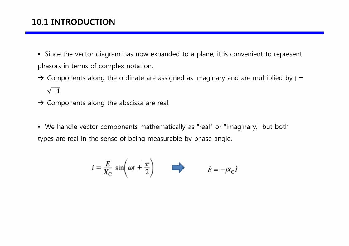
Since the vector diagram has now expanded to a plane, it is convenient to represent

phasors in terms of complex notation.

Components along the ordinate are assigned as imaginary and are multiplied by j

1 .

Components along the abscissa are real.

We handle vector components mathematically as "real" or "imaginary," but both

types are real in the sense of being measurable by phase angle.

10.1 INTRODUCTION

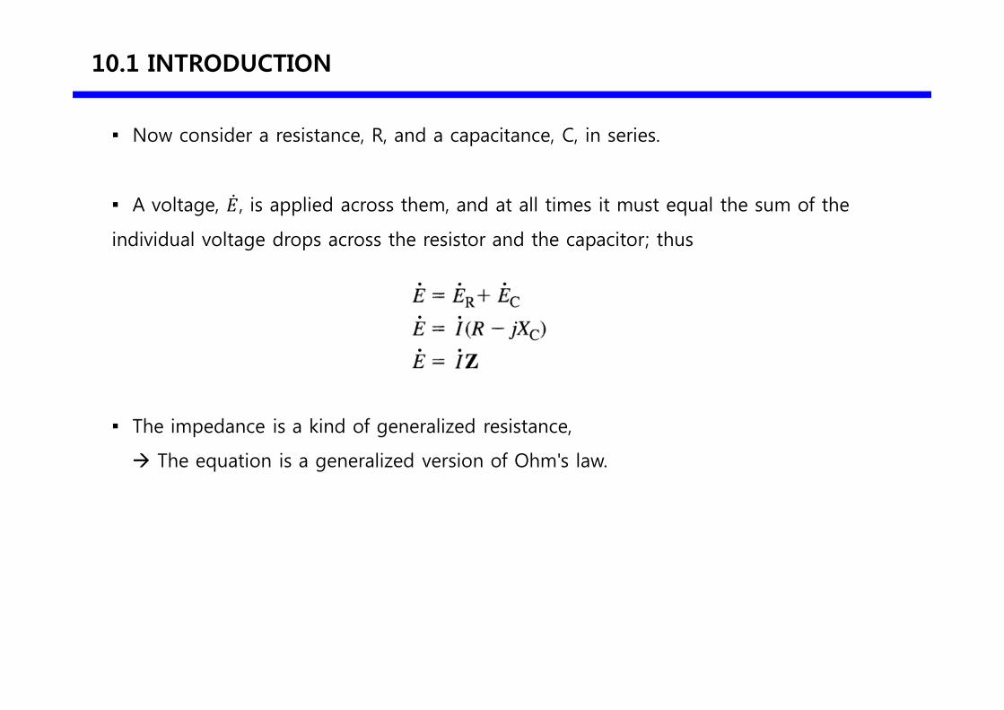
Now consider a resistance, R, and a capacitance, C, in series.

A voltage, , is applied across them, and at all times it must equal the sum of the

individual voltage drops across the resistor and the capacitor; thus

The impedance is a kind of generalized resistance,

The equation is a generalized version of Ohm's law.

10.1 INTRODUCTION

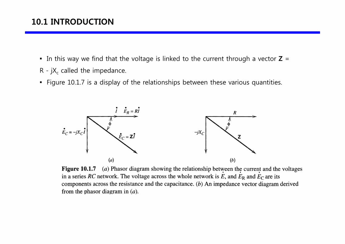
In this way we find that the voltage is linked to the current through a vector Z =

R - jXc called the impedance.

Figure 10.1.7 is a display of the relationships between these various quantities.

10.1 INTRODUCTION

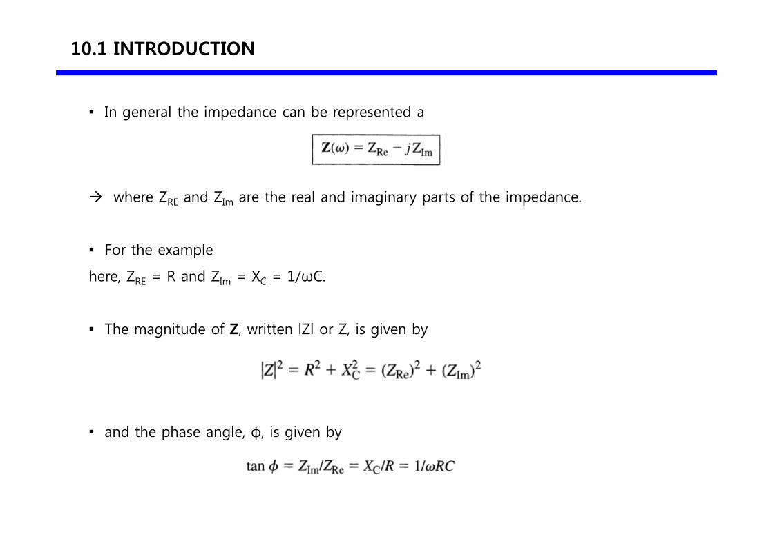
In general the impedance can be represented a

where ZRE and ZIm are the real and imaginary parts of the impedance.

For the example

here, ZRE = R and ZIm = XC = 1/ωC.

The magnitude of Z, written lZl or Z, is given by

and the phase angle, ф, is given by

10.1 INTRODUCTION

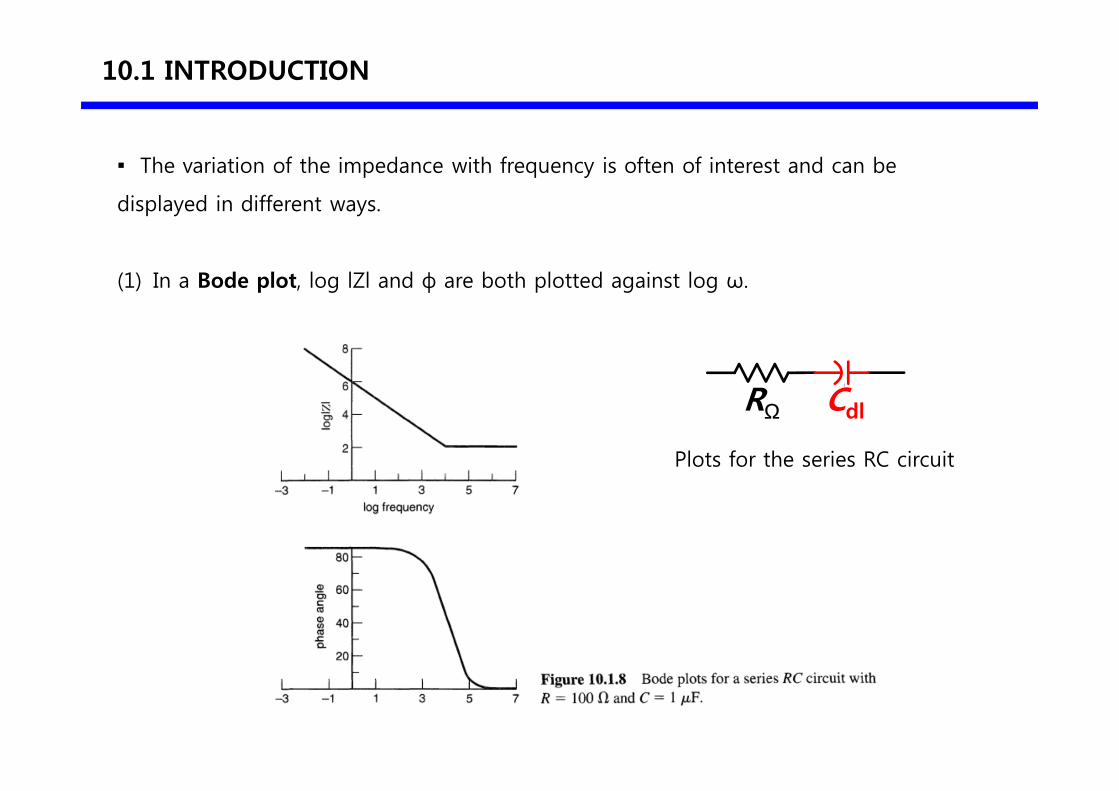
The variation of the impedance with frequency is often of interest and can be

displayed in different ways.

(1) In a Bode plot, log lZl and ф are both plotted against log ω.

Plots for the series RC circuit

RΩ Cdl

10.1 INTRODUCTION

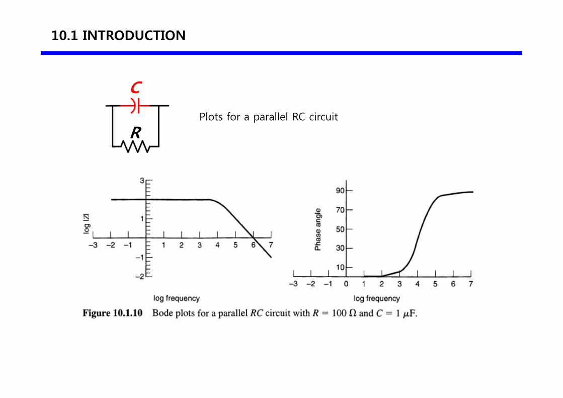
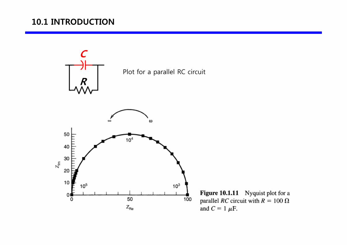
Plots for a parallel RC circuit

R

C

10.1 INTRODUCTION

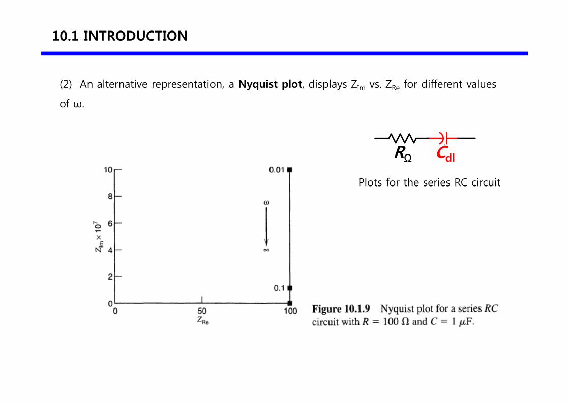
(2) An alternative representation, a Nyquist plot, displays ZIm vs. ZRe for different values

of ω.

Plots for the series RC circuit

RΩ Cdl

10.1 INTRODUCTION

Plot for a parallel RC circuit

R

C

10.1 INTRODUCTION

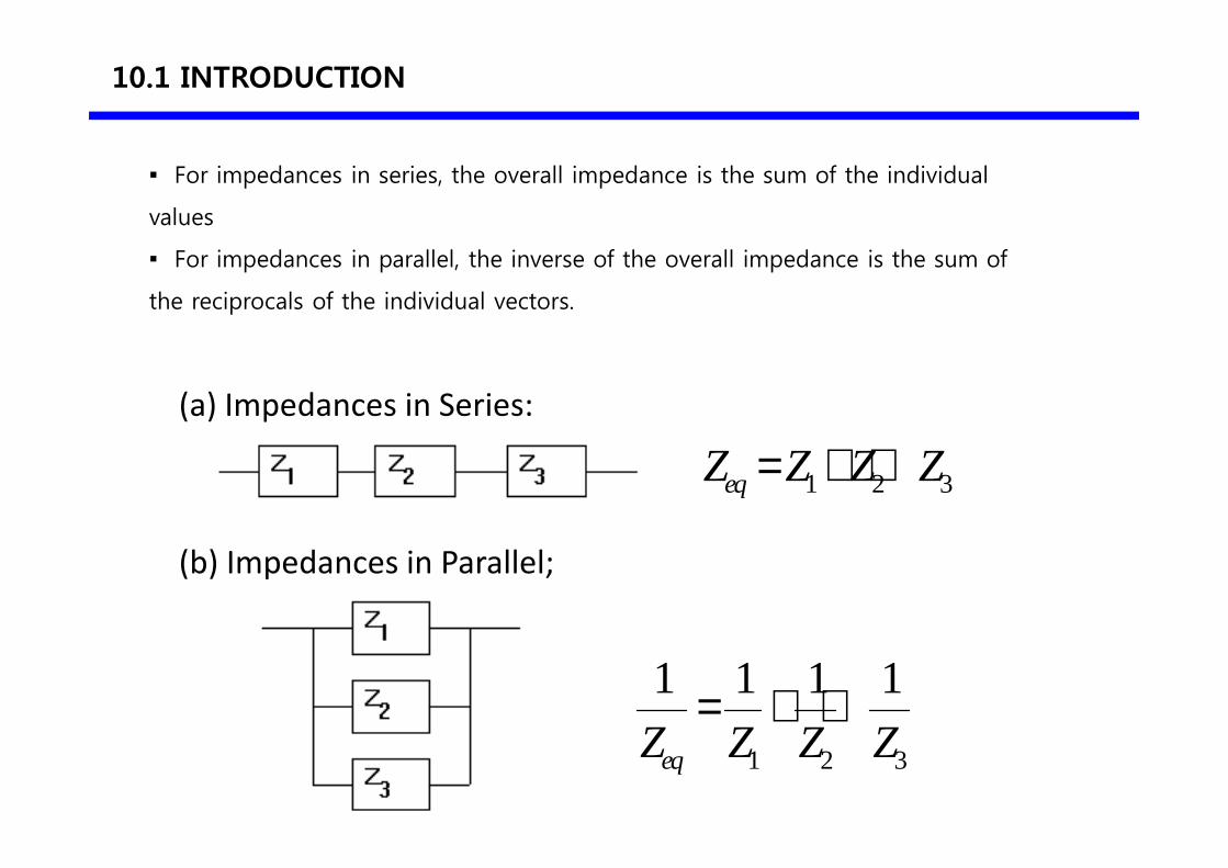
For impedances in series, the overall impedance is the sum of the individual

values

For impedances in parallel, the inverse of the overall impedance is the sum of

the reciprocals of the individual vectors.

(a) Impedances in Series:

1 2 3eqZ Z Z Z= + +

(b) Impedances in Parallel;

1 2 3

1 1 1 1

eqZ Z Z Z= + +

10.1 INTRODUCTION

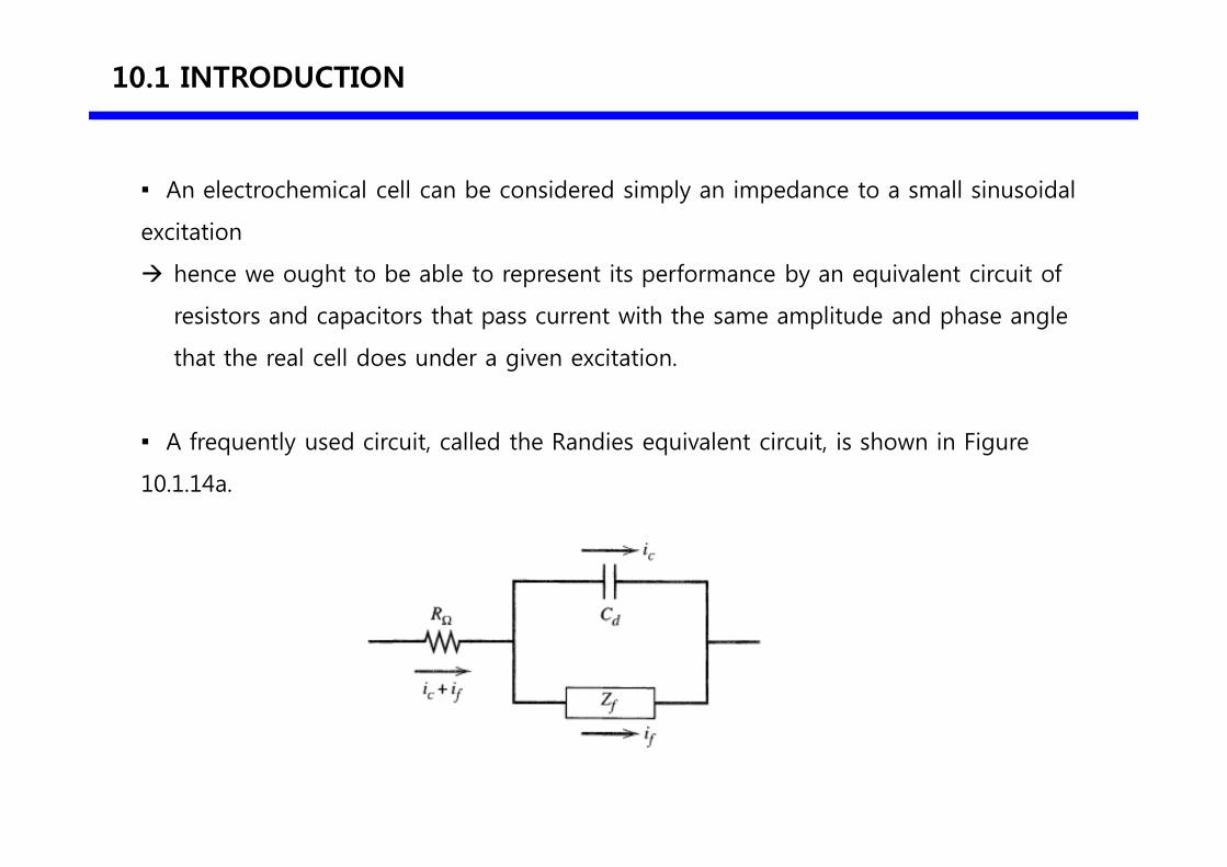
An electrochemical cell can be considered simply an impedance to a small sinusoidal

excitation

hence we ought to be able to represent its performance by an equivalent circuit of

resistors and capacitors that pass current with the same amplitude and phase angle

that the real cell does under a given excitation.

A frequently used circuit, called the Randies equivalent circuit, is shown in Figure

10.1.14a.

10.1 INTRODUCTION

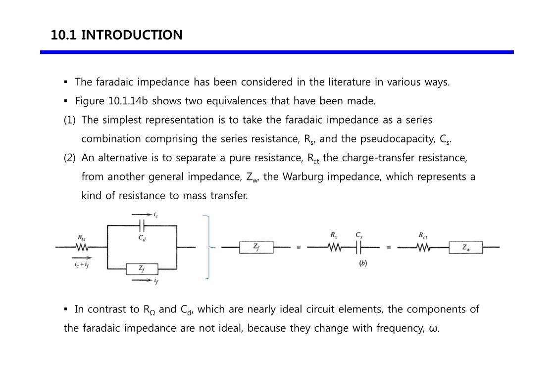
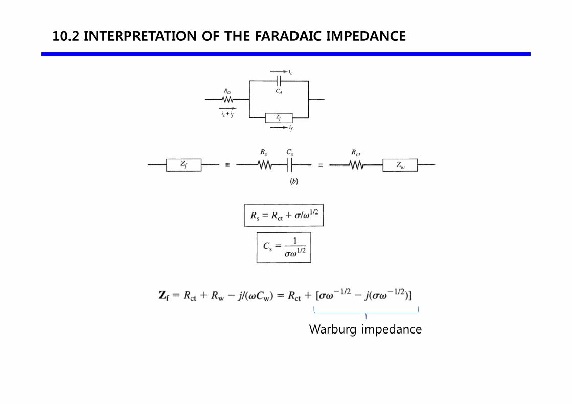
The faradaic impedance has been considered in the literature in various ways.

Figure 10.1.14b shows two equivalences that have been made.

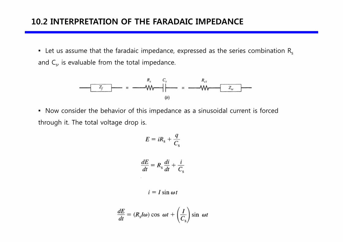
(1) The simplest representation is to take the faradaic impedance as a series

combination comprising the series resistance, Rs, and the pseudocapacity, Cs.

(2) An alternative is to separate a pure resistance, Rct the charge-transfer resistance,

from another general impedance, Zw, the Warburg impedance, which represents a

kind of resistance to mass transfer.

In contrast to RΩ and Cd, which are nearly ideal circuit elements, the components of

the faradaic impedance are not ideal, because they change with frequency, ω.

10.2 INTERPRETATION OF THE FARADAIC IMPEDANCE

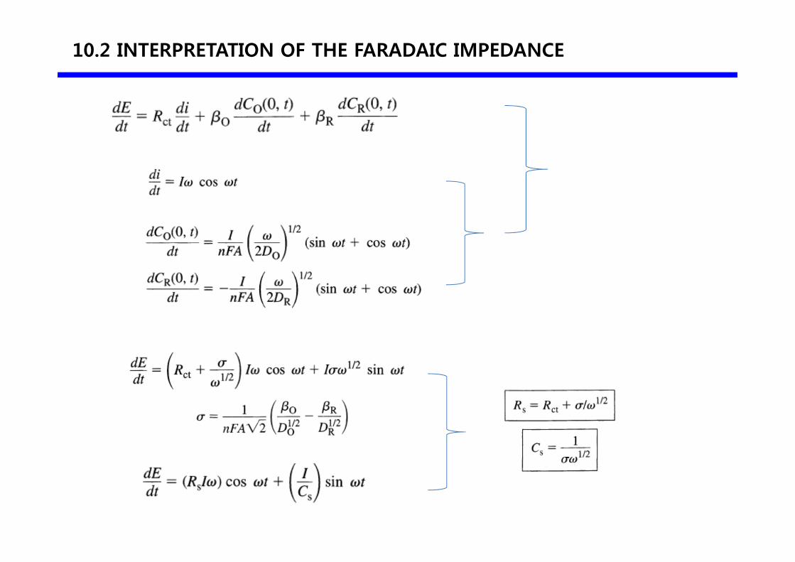
Let us assume that the faradaic impedance, expressed as the series combination Rs

and Cs, is evaluable from the total impedance.

Now consider the behavior of this impedance as a sinusoidal current is forced

through it. The total voltage drop is.


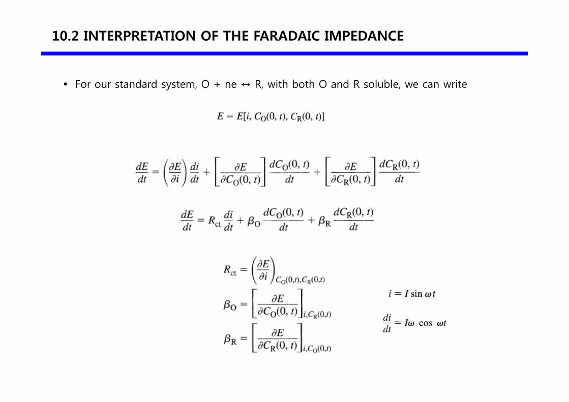
For our standard system, О + ne ↔ R, with both О and R soluble, we can write


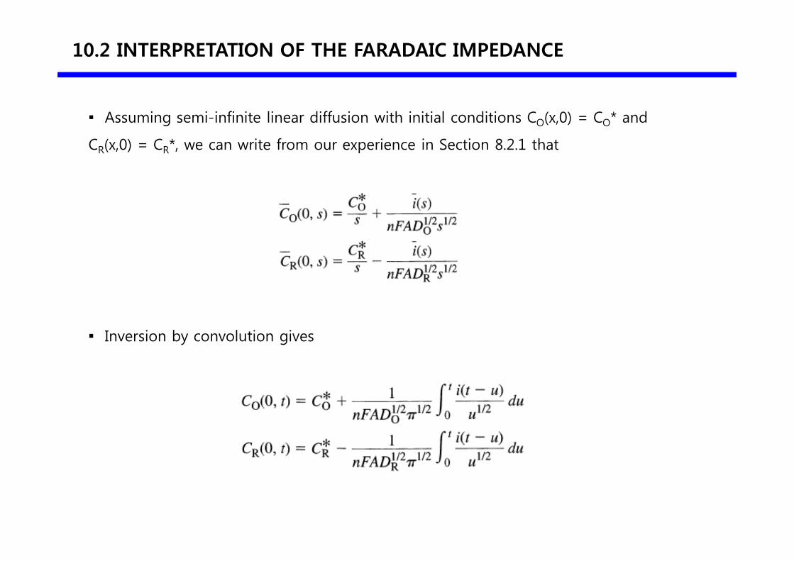
Assuming semi-infinite linear diffusion with initial conditions CO(x,0) = CO* and

CR(x,0) = CR*, we can write from our experience in Section 8.2.1 that

Inversion by convolution gives


=

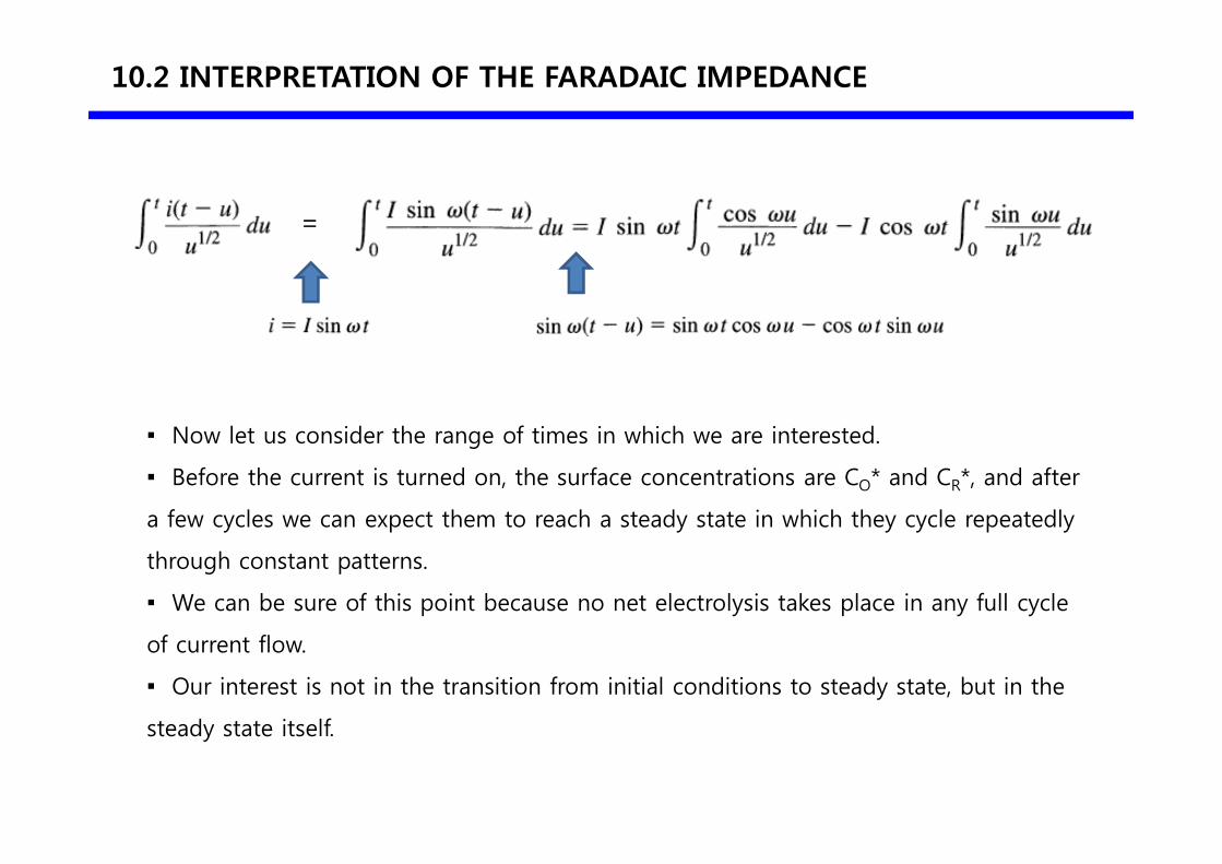
Now let us consider the range of times in which we are interested.

Before the current is turned on, the surface concentrations are CO* and CR*, and after

a few cycles we can expect them to reach a steady state in which they cycle repeatedly

through constant patterns.

We can be sure of this point because no net electrolysis takes place in any full cycle

of current flow.

Our interest is not in the transition from initial conditions to steady state, but in the

steady state itself.


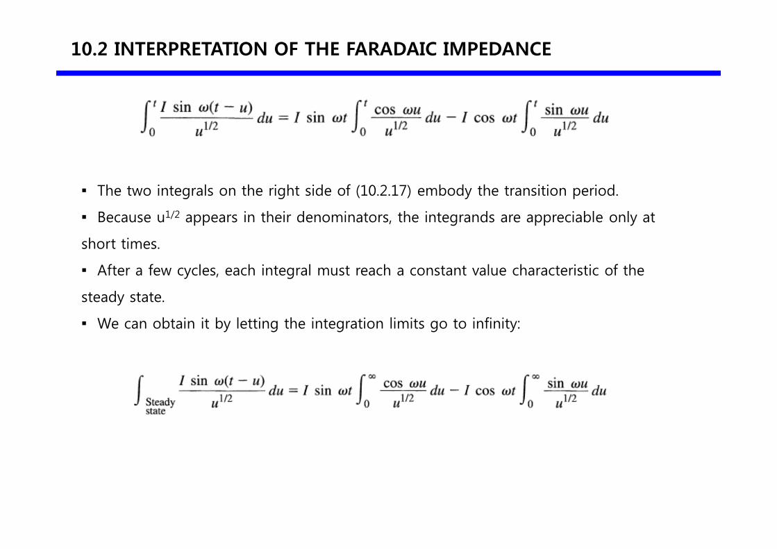
The two integrals on the right side of (10.2.17) embody the transition period.

Because u1/2 appears in their denominators, the integrands are appreciable only at

short times.

After a few cycles, each integral must reach a constant value characteristic of the

steady state.

We can obtain it by letting the integration limits go to infinity:


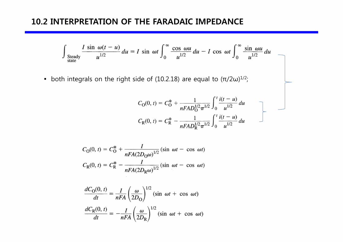
both integrals on the right side of (10.2.18) are equal to (π/2ω)1/2;



Warburg impedance

10.4 ELECTROCHEMICAL IMPEDANCE SPECTROSCOPY

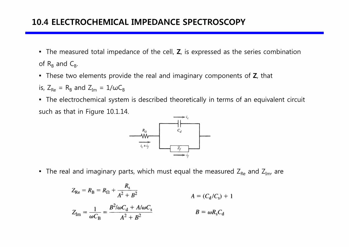
The measured total impedance of the cell, Z, is expressed as the series combination

of RB and CB.

These two elements provide the real and imaginary components of Z, that

is, ZRe = RB and ZIm = 1/ωCB

The electrochemical system is described theoretically in terms of an equivalent circuit

such as that in Figure 10.1.14.

The real and imaginary parts, which must equal the measured ZRe and ZIm, are



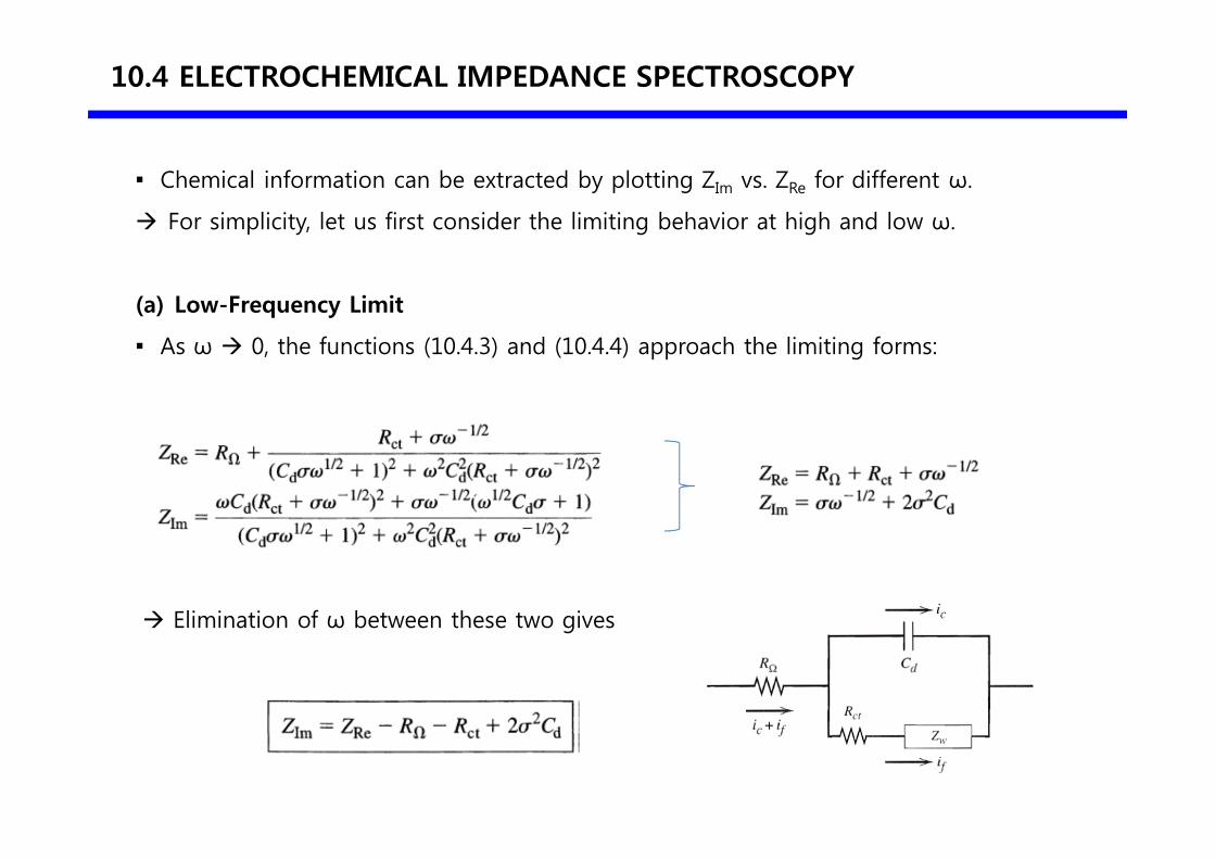
Chemical information can be extracted by plotting ZIm vs. ZRe for different ω.

For simplicity, let us first consider the limiting behavior at high and low ω.

(a) Low-Frequency Limit

As ω 0, the functions (10.4.3) and (10.4.4) approach the limiting forms:

Elimination of ω between these two gives


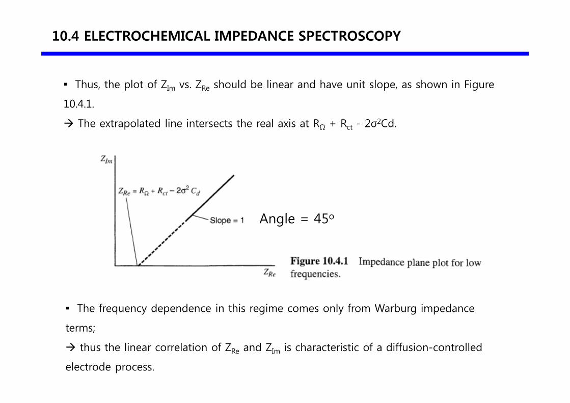
Thus, the plot of ZIm vs. ZRe should be linear and have unit slope, as shown in Figure

10.4.1.

The extrapolated line intersects the real axis at RΩ + Rct - 2σ2Cd.

The frequency dependence in this regime comes only from Warburg impedance

terms;

thus the linear correlation of ZRe and ZIm is characteristic of a diffusion-controlled

electrode process.

Angle = 45o


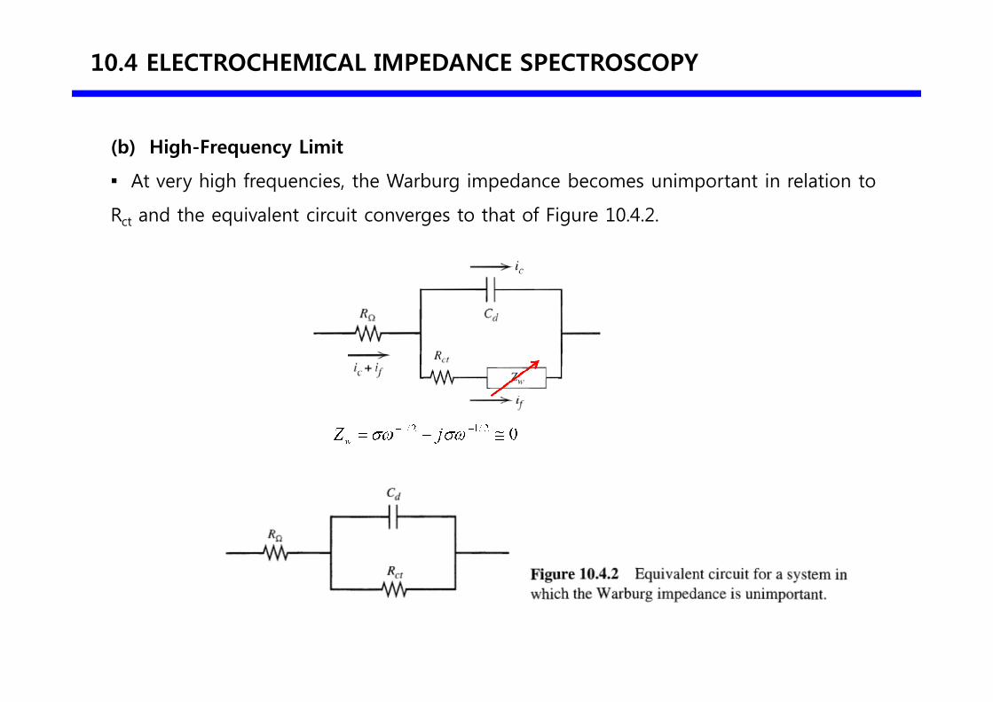
(b) High-Frequency Limit

At very high frequencies, the Warburg impedance becomes unimportant in relation to

Rct and the equivalent circuit converges to that of Figure 10.4.2.


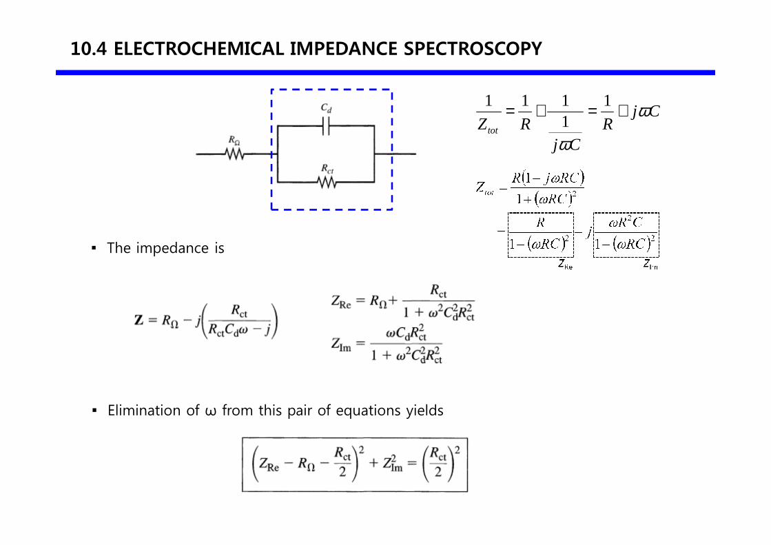
The impedance is

Elimination of ω from this pair of equations yields

CjR

CjRZtot

ω

ω

+=+= 11111


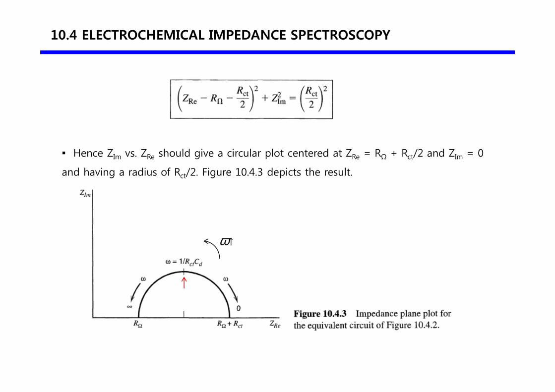
Hence ZIm vs. ZRe should give a circular plot centered at ZRe = RΩ + Rct/2 and ZIm = 0

and having a radius of Rct/2. Figure 10.4.3 depicts the result.

ω↑


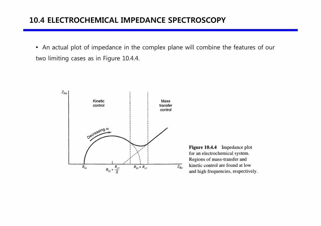
An actual plot of impedance in the complex plane will combine the features of our

two limiting cases as in Figure 10.4.4.

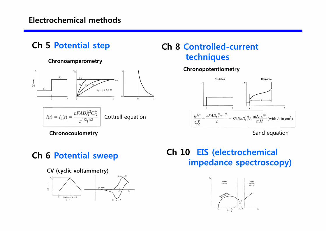
Electrochemical methods

CV (cyclic voltammetry)

Chronopotentiometry

Sand equation

Cottrell equation

Chronoamperometry

Ch 5 Potential step

Chronocoulometry

Ch 8 Controlled-current techniques

Ch 6 Potential sweep Ch 10 EIS (electrochemical impedance spectroscopy)

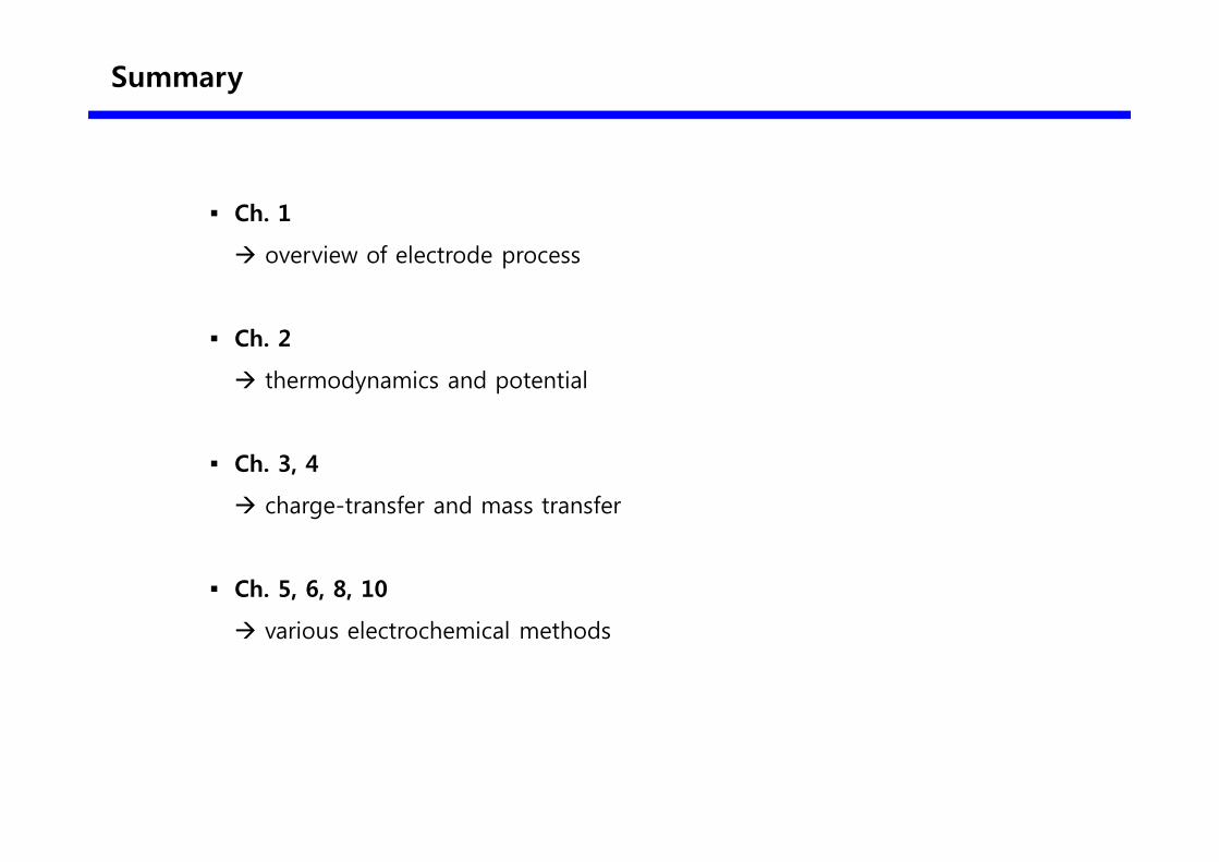
Summary

Ch. 1

overview of electrode process

Ch. 2

thermodynamics and potential

Ch. 3, 4

charge-transfer and mass transfer

Ch. 5, 6, 8, 10

various electrochemical methods

Documents

TECHNIQUES BASED ON CONCEPTS OF IMPEDANCE