TECHNICAL WHITE PAPER: STRUCTURAL & …

OCTOBER 2013 v.2 brain-map.org page 1 of 15 brainspan.org

TECHNICAL WHITE PAPER: STRUCTURAL & CONNECTIONAL IMAGING DATA FOR THE DEVELOPING HUMAN BRAIN OVERVIEW The BrainSpan Atlas of the Developing Human Brain is designed as a foundational resource for studying transcriptional mechanisms involved in human brain development. The resource is the outcome of three ARRA-funded grants through the National Institutes of Health to a consortium consisting of the Allen Institute for Brain Science; Yale University; the University of Southern California; Massachusetts General Hospital, Harvard-MIT Health Sciences and Technology, Athinoula A. Martinos Center for Biomedical Imaging; the University of California, Los Angeles; and the University of Texas Southwestern Medical Center with strong collaborative support from the Genes, Cognition and Psychosis Program, which is part of the Intramural Research Program of NIMH, NIH. All data are publicly accessible via the Allen Brain Atlas data portal at www.brain-map.org or directly at www.brainspan.org. One component of the BrainSpan Atlas is to understand and visualize the three dimensional structure of the developing human brain in order to characterize the structural and connectional properties of the developing brain. This white paper describes the methods and processes used to generate the magnetic resonance imaging data, the diffusion weighted imaging data, and the 3-D fiber tract and developmental transcriptome sampling annotation. The methods for generating other data types included in the BrainSpan atlas are described in separate technical white papers in the Documentation tab. METHODS

Introduction to Ex Vivo Imaging Imaging ex vivo introduces challenges not encountered in the more typical in vivo acquisition. For example, tissue fixation changes most intrinsic magnetic properties of tissue, making sequences that are optimal in vivo inappropriate for ex vivo imaging. To optimize signal-to-noise and contrast-to-noise ratios (SNR and CNR, respectively) special coils were constructed to avoid large spacing between coil elements and sample. Packing procedures immobilized the brain without introducing significant distortion while also making it feasible to place coil elements close to the tissue. Finally, because of the enormous amounts of data produced by the scanning, procedures were implemented for streaming the data off of the scanner to avoid overflowing the scanner database and to allow the k-space data to be reconstructed on a supercomputer with enough memory to implement optimal reconstruction procedures. Below, each of these steps has been detailed pertaining to imaging of the ex vivo 19-24 post-conception weeks (pcw) and adult brains. Sample Packing SNR increases throughout the brain the closer it is to the coil elements. In the case of ex vivo brains, vacuum-sealing samples in polyethylene storage bags, as opposed to using buckets or other containers, is the best way to position the brain as close to the coil elements as possible, while immobilizing the brain to avoid introducing motion-based artifacts into the imaging data. Once packed in a bag, the brain was laid directly against the coil elements as well as easily aligned to avoid an oblique through-plane and/or to place the region of interest in an optimal location relative to the coil. The bagged brain was surrounded and secured by padding to prevent the slight movement the vibrations of the gradients switching cause during the scan. Packing a brain required two people to carefully guide the brain into the bag to avoid losing parts of the brain to the bag's sharp corners. Using a heat sealer, the bag was then sealed on 3 of its 4 sides as tight around the brain as possible. This was to prevent the brain from moving around in the bag as well as to cut down on

http://www.brain-map.org/

http://www.brainspan.org/

http://help.brain-map.org/display/devhumanbrain/Documentation

BRAINSPAN

Technical White Paper: Structural and Connectional Imaging Data for the Developing Human Brain


scan time and data size (the less there was surrounding the brain, the less the scan's field of view must include) as well as to reduce the loading of the coils. Periodate-lysine-paraformaldehyde (PLP) was then added to the bag just above the highest point of the brain. It was challenging to determine the right amount of PLP to use during each packing procedure. If there was too much liquid, it allowed the brain to move around in the bag. If there was too little, it allowed the bag to pucker against the brain causing artifacts in the scan due to magnetic susceptibility differences between air and tissue. The bag was placed in a jar to steady it. This was then placed in a larger bell jar connected to a vacuum in order to evacuate any air bubbles that were trapped in the sulci, vessels, and ventricles of the brain. During vacuuming, the bell jar was agitated manually to help dislodge bubbles. When bubbles were no longer seen making their way to the surface, the vacuum was turned off and the pressure in the bell jar was slowly released. Three people were then needed for the final steps of the brain packing procedure, which involved sealing the top of the bag while keeping the level of liquid in the bag above the brain to prevent exposure to air. A small hole was punctured in the bag in order to vacuum out any remaining air beneath this top seal. A small tube extending from the vacuum (with the addition of a liquid trap to capture any escaping PLP) was placed against the hole. As air was sucked out of the bag, the brain was gently massaged, tapped, and flicked to dislodge more air bubbles from the brain. The challenge was then to seal the bag beneath the hole without allowing air back in while sealing over as little liquid as possible in order to get the front and back of the bag to fuse together. Once secure seals were achieved on all sides, the bag was trimmed as close to the seals as possible. Packing the significantly smaller prenatal brains required only one or two people. An alternative method to packing the prenatal specimen was to surround it with several layers of gauze so it fit snugly in a 500ml tube. PLP was then poured carefully down the edges of the tube until it reached the top. The tube lid was snapped shut and sealed with parafilm to prevent leaks. For one prenatal brain that was provided ex-cranio, it was surrounded with 0.8% agarose gel in a 500ml tube. Agarose was poured into the bottom of the tube and allowed to solidify. The brain was then placed, lateral side down, on top of the solid agarose “base”. Agarose was carefully poured along the edges of the tube, filling in all spaces between the tube and brain. Care was taken to remove air bubbles that formed in the agarose while pouring. This was accomplished by popping the bubbles or pulling them out of the solution with a tissue. The tube lid was snapped shut and sealed with parafilm to prevent any leaks. Coil Design and Construction To achieve the highest spatial resolution (<100 μm isotropic), ex vivo brain imaging typically requires many hours of averaging to recover the SNR that was lost by using such small voxels. Typically, however, a standard clinical in vivo RF coil such as a head array or knee coil is pressed into service. Large arrays of small surface coils are ideal for ex vivo imaging and, depending on the tissue sample size, highly efficient solenoid coils can also produce high quality data as the coil diameter and length can be chosen to place the tissue samples very close to achieve the highest sensitivity over the entire sample, while not violating wavelength limits at a given field strength. With these goals in mind, various coils, namely a 30 channel array coil to image the entire adult brain hemisphere at 7T, solenoid coils that conform to the shape of the prenatal brains both at 3T and 7T were designed and constructed. The 30 channel coil array was tested on a 7T scanner (Siemens Medical Solutions, Erlangen, Germany) with 30 receive channels utilizing a 36 cm diameter head gradient coil. The air/water tight brain container was half of an oblate spheroid (28 cm × 32.5 cm) with a flat top. The brain hemisphere was placed with its flat inter-hemispheric fissure against the flat top. The brain container fits into a fiberglass form of slightly larger dimensions. The bottom half used 16 overlapped circular loop elements and the flat top half uses 14 with a

BRAINSPAN



gap between the two halves. The elements used 5 mm trace widths and diameters of approximately 78 mm (20 elements) and 62 mm (10 elements) and four or five distributed capacitors. A simple lattice balun with a PIN diode detuned each element during transmit. Preamp decoupling was achieved using lumped element phase shifters. Cable traps were placed between the element and preamp. Tuning, matching, and decoupling of neighboring elements was optimized on the bench with the sample in paraformaldehyde solution. Imaging samples in different preservatives required variable matching circuits. Thus, variable capacitors were used to tune and match the coil to different loading properties of the samples. A detunable volume coil (band-pass birdcage, diameter 28 cm, length 20 cm) was used for excitation. The sensitivity of the array was compared with other available coils with high resolution imaging. A 4-turn Solenoid coil (7.5 cm diameter, 9.5 cm length) was used for prenatal specimens for diffusion studies. A 2-turn solenoid coil (6.5 cm inner diameter, 10.5 cm length) with the same electrical characteristics was used to image adult brains at 7T.

Data Streaming and Reconstruction There are several critical engineering issues that arise in high-resolution whole-brain scanning using the Siemens scanners. First, the data quantity acquired was too large to be processed into images by the scanner software itself. Instead, custom software was necessary to transform the measured data into a series of image volumes. Challenges in this stage included performing the inverse Fourier transform in a resource-efficient manner given the large dataset, and also determining the optimal combination of signals for each element of the receive coil. However, even before data reconstruction was considered, another set of problems was encountered. In particular, the measured dataset for a single volume was so large that the buffer hard disks on the scanner could not hold them. To get around this, custom pulse sequence software was written that measures k-space in "chunks" that are small enough to be held on the buffer. Additionally, a system was developed that streams each "chunk" of data from the buffer to a multi-terabyte RAID array in parallel with it being measured by the scanner. This parallelism was essential so that the buffer can be immediately wiped at the end of each scan and the next scan can begin filling it again, without time being wasted transferring data while no scanning was occurring. Due to the large bandwidth requirements of this streaming system, and the demands for reliability implied by multi-day scan sessions, a substantial amount of systems integration work was required to establish fast, reliable network and RAID connections, and custom software was developed to ensure that there was minimal overhead in the data stream as it passed through the system. Once the images from each coil channel had been reconstructed, they were combined into a single image. The standard approach for this combination was the root-sum-of-squares method, which generates a single magnitude image from the set of complex-valued individual coil channel images. This combination, however, does not take into account the varying levels of additive thermal noise measured across the coil elements. To maximize the image signal-to-noise ratio in the combined image requires extra information about the noise seen by each coil. The optimal SNR combination (Roemer et al., 1990) incorporates extra information about the coil array in the form of estimates of both the spatial sensitivity profiles of the coil elements (i.e., the signal) and the coupling of thermal noise across the channels (i.e., the noise). This weighted combination directly maximizes the SNR in the combined image. In practice, estimating the coil sensitivity profiles accurately can be difficult and time-consuming, however estimating the coil noise covariance matrix was fast, straightforward, and provides most of the SNR boost given by the optimal SNR combination. For our image reconstruction pipeline, we perform a noise-weighted combination as an approximation to the optimal SNR combination. The noise covariance matrix for a coil array was estimated from a noise-only measurement collected in the absence of any RF excitation. This acquisition lasts about 20 seconds and provides enough thermal noise samples to accurately estimate the noise covariance matrix for the 32-channel coil and describes the thermal noise coupling between the individual coil channel images for un-accelerated acquisitions. The final combined image was then computed as a noise-weighted sum of the complex-valued individual coil channel images and was given by

BRAINSPAN



ssI 1H Ψ where I represents the combined image intensity at a given pixel, Ψ represents the N×N noise covariance matrix, and s represents the N×1 vector of complex-valued image intensities at a given pixel across the N coils of the array (Roemer et al., 1990; Wright & Wald, 1997). Note that the root-sum-of-squares combination was a special case of the noise-weighted combination when the noise covariance matrix was the identity matrix. For coil arrays with a small number of elements (e.g., four), the noise covariance matrix can be similar enough to the identity matrix such that the root-sum-of-squares combination yields a close approximation to the optimal SNR combination (Roemer et al., 1990). As the number of coil elements increases, however, this noise covariance matrix deviates substantially from the identity matrix, which can lead to a significant boost in SNR in some cases (Wiggins et al., 2008). Furthermore, at high fields such as 7T, the noise coupling between elements can increase due to cross-talk induced by cable currents, which will also contribute to the deviation of the noise covariance matrix from the identity matrix (Wald et al., 2005). Thus, performing a noise-weighted combination of high-field magnetic resonance imaging (MRI) data acquired with multi-channel receive coil arrays can provide increased SNR with only a negligible additional acquisition time and a straightforward modification to the image reconstruction pipeline. Structural Sequence Design MRI is an enormously flexible technology that allows contrast to be generated using various endogenous magnetic properties of tissue as well as the density of water protons occurring at each point in space. Designing acquisitions typically means finding parameters that optimize the CNR per unit time between relevant tissue types. In the present example, the CNR/unit time for gray and white matter was optimized in order to distinguish these tissues as well as to discern laminar intracortical architecture. In order to determine optimal parameters for gray/white CNR per-unit-time, data was acquired spanning the range of likely optimal parameters and also allowed us to perform Bloch equation-based parameter-estimation. This enabled the use of a forward model of image formation to synthesize signals with arbitrary (gradient-echo) images and exhaustively search for optimal imaging parameters. Figure 1 shows an example of this acquisition type, which compares an adult sample with a 19 pcw sample, both acquired at 7T with 200µm isotropic voxels and a 20° flip angle.

Figure 1. Acquisition of 7T with 200 µm isotropic voxels and a 20° flip angle. Comparison of an adult (left) and

prenatal (19 pcw) (right) 20° FLASH scan.

By acquiring data with varying flip angles, parameter estimation procedures (Fischl et al., 2004) were used to solve for the intrinsic magnetic tissue properties, T1, T2* and proton density (PD) that optimally explained the

BRAINSPAN



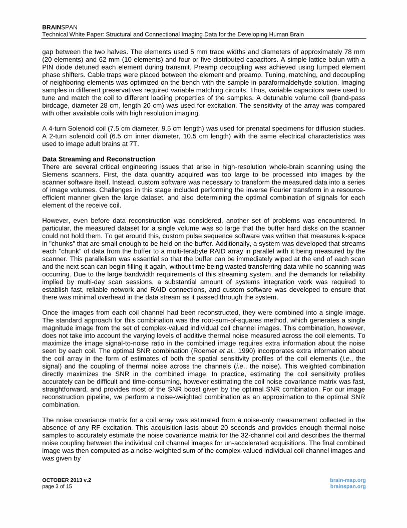
observed imaging data. An example of the parameter maps generated by this technique is shown in Figure 2 for the same samples. This example highlights differences between the adult and developing brain, where contrast that was optimal in the adult was completely incorrect in the prenatal sample due presumably to myelination differences.

Figure 2. T1 parameter maps for the adult (left) and a prenatal (19 pcw, right) brains.

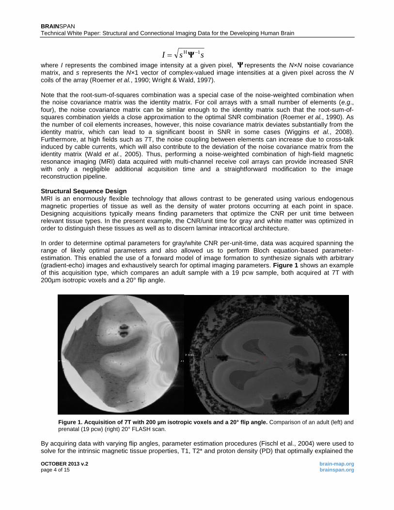
Labels were manually drawn in the gray matter and white matter of the two samples to compute MR parameters that would result in optimal CNR/unit time. This was accomplished by using the labeled values as inputs to the Bloch equations (Bloch 1946) to predict image intensities, then dividing by the square root of the sequence length (governed by the repetition time TR). The differences in T1 in the white matter in the adult and prenatal samples, shown in Figure 3, left panel, implied that different imaging parameters were required to optimally image the prenatal samples. This was predicted by the results of the simulation, shown in Figure 3, right panel, in which for a given TR large flip angle, which emphasizes T1 contrast as opposed to proton density, higher CNR is produced.

Figure 3. Differences in T1 in the adult and prenatal samples predict that different imaging parameters are required to optimally image the prenatal samples. Left panel shows the mean T1 values for different tissue

types (white matter and gray matter) in the prenatal 19 pcw (red) and adult (blue) samples. Right panel shows the optimal CNR for different length acquisitions.

BRAINSPAN



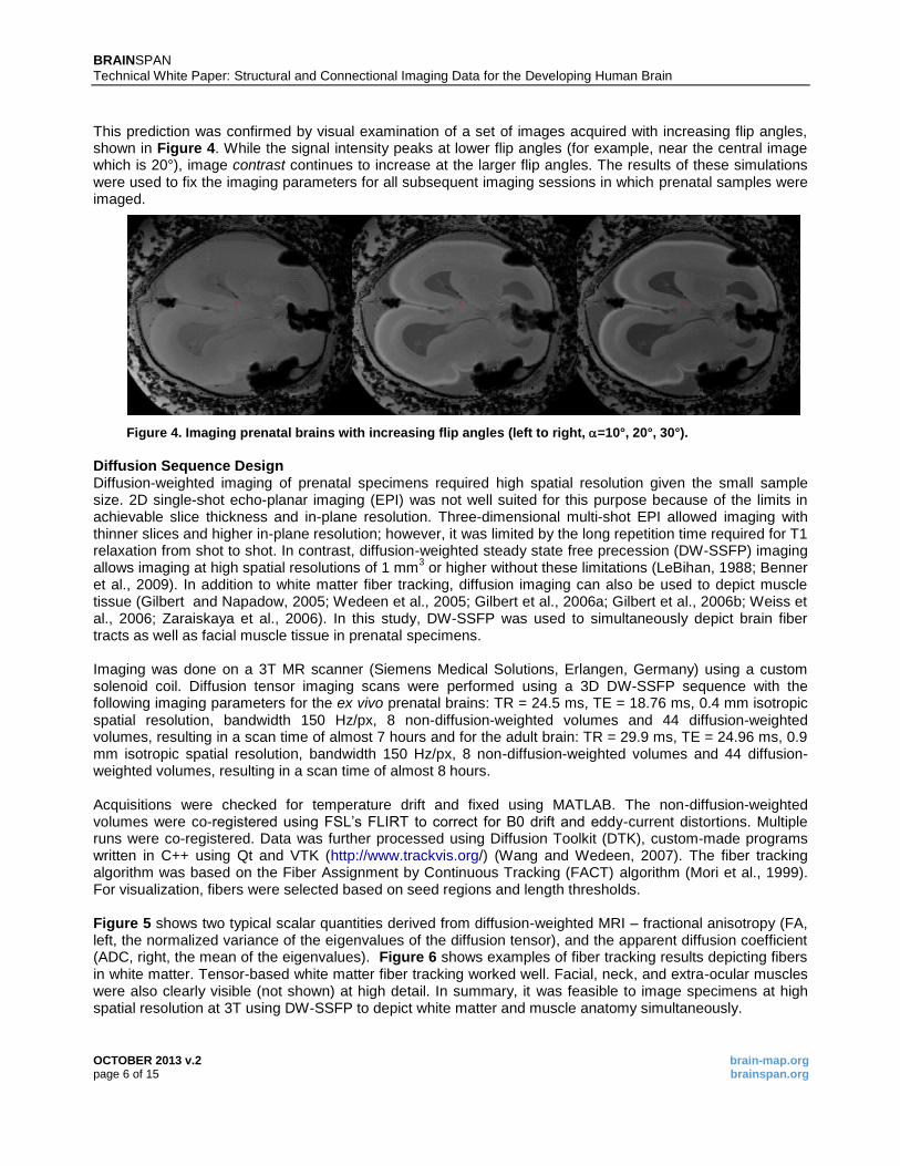
This prediction was confirmed by visual examination of a set of images acquired with increasing flip angles, shown in Figure 4. While the signal intensity peaks at lower flip angles (for example, near the central image which is 20°), image contrast continues to increase at the larger flip angles. The results of these simulations were used to fix the imaging parameters for all subsequent imaging sessions in which prenatal samples were imaged.

Figure 4. Imaging prenatal brains with increasing flip angles (left to right, =10°, 20°, 30°).

Diffusion Sequence Design Diffusion-weighted imaging of prenatal specimens required high spatial resolution given the small sample size. 2D single-shot echo-planar imaging (EPI) was not well suited for this purpose because of the limits in achievable slice thickness and in-plane resolution. Three-dimensional multi-shot EPI allowed imaging with thinner slices and higher in-plane resolution; however, it was limited by the long repetition time required for T1 relaxation from shot to shot. In contrast, diffusion-weighted steady state free precession (DW-SSFP) imaging allows imaging at high spatial resolutions of 1 mm

3 or higher without these limitations (LeBihan, 1988; Benner

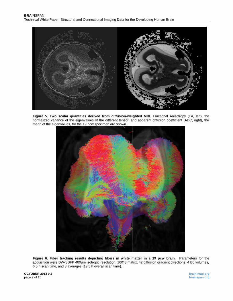
et al., 2009). In addition to white matter fiber tracking, diffusion imaging can also be used to depict muscle tissue (Gilbert and Napadow, 2005; Wedeen et al., 2005; Gilbert et al., 2006a; Gilbert et al., 2006b; Weiss et al., 2006; Zaraiskaya et al., 2006). In this study, DW-SSFP was used to simultaneously depict brain fiber tracts as well as facial muscle tissue in prenatal specimens. Imaging was done on a 3T MR scanner (Siemens Medical Solutions, Erlangen, Germany) using a custom solenoid coil. Diffusion tensor imaging scans were performed using a 3D DW-SSFP sequence with the following imaging parameters for the ex vivo prenatal brains: TR = 24.5 ms, TE = 18.76 ms, 0.4 mm isotropic spatial resolution, bandwidth 150 Hz/px, 8 non-diffusion-weighted volumes and 44 diffusion-weighted volumes, resulting in a scan time of almost 7 hours and for the adult brain: TR = 29.9 ms, TE = 24.96 ms, 0.9 mm isotropic spatial resolution, bandwidth 150 Hz/px, 8 non-diffusion-weighted volumes and 44 diffusion-weighted volumes, resulting in a scan time of almost 8 hours. Acquisitions were checked for temperature drift and fixed using MATLAB. The non-diffusion-weighted volumes were co-registered using FSLʼs FLIRT to correct for B0 drift and eddy-current distortions. Multiple runs were co-registered. Data was further processed using Diffusion Toolkit (DTK), custom-made programs written in C++ using Qt and VTK (http://www.trackvis.org/) (Wang and Wedeen, 2007). The fiber tracking algorithm was based on the Fiber Assignment by Continuous Tracking (FACT) algorithm (Mori et al., 1999). For visualization, fibers were selected based on seed regions and length thresholds. Figure 5 shows two typical scalar quantities derived from diffusion-weighted MRI – fractional anisotropy (FA, left, the normalized variance of the eigenvalues of the diffusion tensor), and the apparent diffusion coefficient (ADC, right, the mean of the eigenvalues). Figure 6 shows examples of fiber tracking results depicting fibers in white matter. Tensor-based white matter fiber tracking worked well. Facial, neck, and extra-ocular muscles were also clearly visible (not shown) at high detail. In summary, it was feasible to image specimens at high spatial resolution at 3T using DW-SSFP to depict white matter and muscle anatomy simultaneously.

BRAINSPAN



Figure 5. Two scalar quantities derived from diffusion-weighted MRI. Fractional Anisotropy (FA, left), the

normalized variance of the eigenvalues of the different tensor, and apparent diffusion coefficient (ADC, right), the mean of the eigenvalues, for the 19 pcw specimen are shown.

Figure 6. Fiber tracking results depicting fibers in white matter in a 19 pcw brain. Parameters for the

acquisition were DW-SSFP 400µm isotropic resolution, 160^3 matrix, 42 diffusion gradient directions, 4 B0 volumes, 6.5 h scan time, and 3 averages (19.5 h overall scan time).

BRAINSPAN



19 pcw

7T

Session name: 19wg_bay5_scan3

MEF, twelve echoes, 3 runs/flip 200um, flips angles 20°, 40°, 60°, 80°

TE (Echo Time in ms) = 4.23, 7.53, 10.83, 14.13, 17.43, 20.73, 24.03, 27.33, 30.63, 33.93, 37.23, 40.53

TR (Repetition Time in ms) = 49

3T


MEF 5 runs/flip 500um flips 10°, 20°, 30°, 40°, 50°, 60°

TE (Echo Time ms) = 2.93, 5.83, 8.93, 12.23, 15.73, 19.43

TR (Repetition Time, ms) = 25

T2_SPACE 5 runs 500um

MEF, 1mm, 8 echoes, 1 run/flip angles 5°, 10°, 15°, 20°, 25°, 30°

TE (Echo Time ms) = 1.85, 3.85, 5.85, 7.85, 9.85, 11.85, 13.85, 15.85

TR (Repetition Time ms) = 20

Diffusion 400um 5 runs, 44 directions

21 pcw

7T

Session name: 21wg_bay5

MEF 12e 3 runs/flip 200um flips 20°, 40°, 60°, 80°

TE (Echo Time, ms) = 4.23, 7.53, 10.83, 14.13, 17.43, 20.73, 24.03, 27.33, 30.63, 33.93, 37.23, 40.53


3T

Session name: 21wg bay6 (3T)

MEF 6 echoes, 6 runs/flip, 500um flips 10°, 20°, 30°, 40°, 50°, 60°

TE (Echo Time ms) = 2.93, 5.83, 8.93, 12.23, 15.73, 19.43


T2_SPACE 5 runs 500um

Diffusion 400um 2 runs, 44 directions; 250um 1 run

22 pcw

7T

Session name: 22wg_bay5_scan3:

MEF 3 runs/flip 200um flips 20°, 40°, 60°, 80°

TE (Echo Time, ms) = 4.23, 7.53, 10.83, 14.13, 17.43, 20.73, 24.03, 27.33, 30.63, 33.93, 37.23, 40.53


3T


MEF 5 runs/flip 500um flips 10°, 20°, 30°, 40°, 50°, 60°

TE (Echo Time ms) = 3.55, 6.45, 9.55, 12.85, 16.35, 20.05


T2SPACE 5 runs 500um

Diffusion 400um 2 runs, 44 directions

Adult (34 years)

7T

Session name: AllenAdult02_bay5

MEF 1 run/flip 200um flips 20°, 40°, 60°, 80°

TE (Echo Time ms) = 5.49, 12.84, 20.19, 27.60, 35.20, 42.80


3T

Session name: AllenAdult02_bay6_scan3

MEF 6 echoes, 1mm 1 run/flip, flips 10°, 20°, 30°, 40°, 50°, 60°

TE (Echo Time ms) = 2.93, 5.83, 8.93, 12.23, 15.73, 19.43


1 run T2SPACE

Diffusion: 2 runs 900um, 60 directions

2 runs at 1200um Table 1. T7 and T3 acquired data

BRAINSPAN



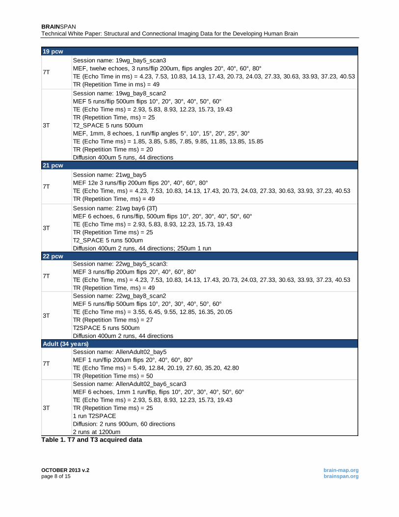
Description of Individual Datasets The data acquired for each sample on the 7T and 3T scanners is listed in Table 1. MEF indicates multi-echo FLASH acquisitions. In each case, the need to increase resolution while maintaining good SNR in the available scan time was balanced. Prenatal brains were all imaged in solenoid receive coils custom built for this project, while the adult brains were imaged in a custom-build 32 channel array at 7T, and a standard Siemens 32 channel array at 3T. 3-D FIBER TRACT AND DEVELOPMENTAL TRANSCRIPTOME SAMPLING ANNOTATION Prenatal brain specimens and postnatal healthy subjects The age, gender and race information of the prenatal brain specimens and postnatal healthy subjects that were utilized for annotation are shown in Table 2. None of these specimens overlap with the specimens described in the previous method sections.

Table 2. Prenatal brain samples and postnatal healthy subjects

Age 14 pcw 17 pcw 19 pcw 37 pcw 3 yrs 8 yrs 15 yrs 32 yrs

Gender F M n/a F M M F M

Race Caucasian Caucasian Caucasian Hispanic Asian Caucasian Asian Asian

Shaded time points indicate samples are from postmortem specimens. Abbreviations: pcw, post-conception weeks; Y, postnatal years; F, female; M, male; n/a, not available.

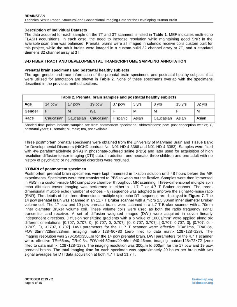
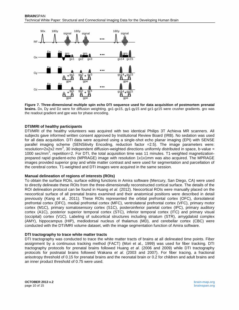
Three postmortem prenatal specimens were obtained from the University of Maryland Brain and Tissue Bank for Developmental Disorders (NICHD contract No. N01-HD-4-3368 and N01-HD-4-3383). Samples were fixed with 4% paraformaldehyde (PFA) in phosphate-buffered saline (PBS) and later used for acquisition of high resolution diffusion tensor imaging (DTI) data. In addition, one neonate, three children and one adult with no history of psychiatric or neurological disorders were recruited. DTI/MRI of postmortem specimen Postmortem prenatal brain specimens were kept immersed in fixation solution until 48 hours before the MR experiments. Specimens were then transferred to PBS to wash out the fixative. Samples were then immersed in PBS in a custom-made MR compatible chamber throughout MR scanning. Three-dimensional multiple spin echo diffusion tensor imaging was performed in either a 11.7 T or 4.7 T Bruker scanner. The three-dimensional multiple echo (number of echoes = 8) sequence was adopted to improve the signal-to-noise ratio (SNR). The details of this three-dimensional multiple spin echo DTI sequence are displayed in Figure 7. The 14 pcw prenatal brain was scanned in an 11.7 T Bruker scanner with a micro 2.5 30mm inner diameter Bruker volume coil. The 17 pcw and 19 pcw prenatal brains were scanned in a 4.7 T Bruker scanner with a 70mm inner diameter Bruker volume coil. These volume coils were used as both the radio frequency signal transmitter and receiver. A set of diffusion weighted images (DWI) were acquired in seven linearly independent directions. Diffusion sensitizing gradients with a b value of 1000s/mm

2 were applied along six

different orientations: [0.707, 0.707, 0], [0.707, 0, 0.707], [0, 0.707, 0.707], [-0.707, 0.707, 0], [0.707, 0, -0.707], [0, -0.707, 0.707]. DWI parameters for the 11.7 T scanner were: effective TE=67ms, TR=0.8s, FOV=35mm/28mm/28mm, imaging matrix=128×80×80 (zero filled to data matrix=128×128×128). The

imaging resolution was 273x350x350m for the 14 pcw prenatal brain. DWI parameters for the 4.7 T scanner were: effective TE=66ms, TR=0.8s, FOV=44-52mm/40-46mm/40-46mm, imaging matrix=128×72×72 (zero

filled to data matrix=128×128×128). The imaging resolution was 300m to 600m for the 17 pcw and 19 pcw prenatal brains. The total imaging time for each specimen was approximately 20 hours per brain with two signal averages for DTI data acquisition at both 4.7 T and 11.7 T.

BRAINSPAN



•••

+ + +

+ + +

90x 180y 180y 180ysignal signal signal

RF

Gx

Gy

Gz

Dx Dx

Dy Dy

Dz Dz

gro gro gro

gx1

gpe gpe gpe

gpe gpe gpe

gx2 gx3 gx14 gx15

gy1 gy2 gy3 gy14 gy15

gz1 gz2 gz3 gz14 gz15

•••

•••

•••

Figure 7. Three-dimensional multiple spin echo DTI sequence used for data acquisition of postmortem prenatal brains. Dx, Dy and Dz were for diffusion weighting. gx1-gx15, gy1-gy15 and gz1-gz15 were crusher gradients. gro was

the readout gradient and gpe was for phase encoding.

DTI/MRI of healthy participants DTI/MRI of the healthy volunteers was acquired with two identical Philips 3T Achieva MR scanners. All subjects gave informed written consent approved by Institutional Review Board (IRB). No sedation was used for all data acquisition. DTI data were acquired using a single-shot echo planar imaging (EPI) with SENSE parallel imaging scheme (SENSitivity Encoding, reduction factor =2.5). The image parameters were: resolution=2x2x2 mm

3, 30 independent diffusion-weighted directions uniformly distributed in space, b-value =

1000 sec/mm2, repetition=2. For DTI, the total acquisition time was 11 minutes. T1-weighted magnetization-

prepared rapid gradient-echo (MPRAGE) image with resolution 1x1x1mm was also acquired. The MPRAGE images provided superior gray and white matter contrast and were used for segmentation and parcellation of the cerebral cortex. T1-weighted and DTI images were acquired in the same session. Manual delineation of regions of interests (ROIs) To obtain the surface ROIs, surface editing functions in Amira software (Mercury, San Diego, CA) were used to directly delineate these ROIs from the three-dimensionally reconstructed cortical surface. The details of the ROI delineation protocol can be found in Huang et al. (2012). Neocortical ROIs were manually placed on the neocortical surface of all prenatal brains examined and their anatomical positions were described in detail previously (Kang et al., 2011). These ROIs represented the orbital prefrontal cortex (OFC), dorsolateral prefrontal cortex (DFC), medial prefrontal cortex (MFC), ventrolateral prefrontal cortex (VFC), primary motor cortex (M1C), primary somatosensory cortex (S1C), posteroinferior parietal cortex (IPC), primary auditory cortex (A1C), posterior superior temporal cortex (STC), inferior temporal cortex (ITC) and primary visual (occipital) cortex (V1C). Labeling of subcortical structures including striatum (STR), amygdaloid complex (AMY), hippocampus (HIP), mediodorsal nucleus of thalamus (MD), and cerebellar cortex (CBC) were conducted with the DTI/MRI volume dataset, with the image segmentation function of Amira software. DTI tractography to trace white matter tracts DTI tractography was conducted to trace the white matter tracts of brains at all delineated time points. Fiber assignment by a continuous tracking method (FACT) (Mori et al., 1999) was used for fiber tracking. DTI tractography protocols for prenatal brains followed Huang et al. (2006 and 2009) while DTI tractography protocols for postnatal brains followed Wakana et al. (2003 and 2007). For fiber tracing, a fractional anisotropy threshold of 0.15 for prenatal brains and the neonatal brain or 0.2 for children and adult brains and an inner product threshold of 0.75 were used.

BRAINSPAN



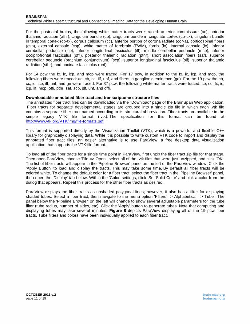
For the postnatal brains, the following white matter tracts were traced: anterior commissure (ac), anterior thalamic radiation (athf), cingulum bundle (cb), cingulum bundle in cingulate cortex (cb-cx), cingulum bundle in temporal cortex (cb-tx), corpus callosum (cc), anterior portion of corona radiate (cor-a), corticospinal fibers (csp), external capsule (csp), white matter of forebrain (FWM), fornix (fx), internal capsule (ic), inferior cerebellar peduncle (icp), inferior longitudinal fasciculus (ilf), middle cerebellar peduncle (mcp), inferior occipitofrontal fasciculus (offi), posterior thalamic radiation (pthr), short association fibers (saf), superior cerebellar peduncle (brachium conjunctivum) (scp), superior longitudinal fasciculus (slf), superior thalamic radiation (sthr), and uncinate fasciculus (unf). For 14 pcw the fx, ic, icp, and mcp were traced. For 17 pcw, in addition to the fx, ic, icp, and mcp, the following fibers were traced: ac, cb, cc, ilf, unf, and fibers in ganglionic eminence (ge). For the 19 pcw the cb, cc, ic, icp, ilf, unf, and ge were traced. For 37 pcw, the following white matter tracts were traced: cb, cc, fx, ic, icp, ilf, mcp, offi, pthr, saf, scp, slf, unf, and offi. Downloadable annotated fiber tract and transcriptome structure files The annotated fiber tract files can be downloaded via the "Download" page of the BrainSpan Web application. Fiber tracts for separate developmental stages are grouped into a single zip file in which each .vtk file contains a separate fiber tract named according to its structural abbreviation. Fiber tracts are available in the simple legacy VTK file format (.vtk). The specification for this format can be found at http://www.vtk.org/VTK/img/file-formats.pdf. This format is supported directly by the Visualization Toolkit (VTK), which is a powerful and flexible C++ library for graphically displaying data. While it is possible to write custom VTK code to import and display the annotated fiber tract files, an easier alternative is to use ParaView, a free desktop data visualization application that supports the VTK file format. To load all of the fiber tracts for a single time point in ParaView, first unzip the fiber tract zip file for that stage. Then open ParaView, choose 'File => Open', select all of the .vtk files that were just unzipped, and click 'OK'. The list of fiber tracts will appear in the 'Pipeline Browser' panel on the left of the ParaView window. Click the 'Apply Button' to load and display the tracts. This may take some time. By default all fiber tracts will be colored white. To change the default color for a fiber tract, select the fiber tract in the 'Pipeline Browser' panel, then open the 'Display' tab below. Within the 'Color' settings, click 'Set Solid Color' and pick a color from the dialog that appears. Repeat this process for the other fiber tracts as desired. ParaView displays the fiber tracts as unshaded polygonal lines; however, it also has a filter for displaying shaded tubes. Select a fiber tract, then navigate to the menu option 'Filters => Alphabetical => Tube'. The panel below the 'Pipeline Browser' on the left will change to show several adjustable parameters for the tube filter (tube radius, number of sides, etc). Click the 'Apply' button to generate tubes. Note that computing and displaying tubes may take several minutes. Figure 8 depicts ParaView displaying all of the 19 pcw fiber tracts. Tube filters and colors have been individually applied to each fiber tract.

http://www.vtk.org/VTK/img/file-formats.pdf

BRAINSPAN



Figure 8. A depiction of ParaView displaying all of the 19 pcw fiber tracts. Tube filters and colors have been individually

applied to each fiber tract.

Structures sampled in the developmental transcriptome (OFC, DFC, MFC, VFC, M1C, S1C, IPC, A1C, STC, ITC, V1C, STR, AMY, HIP, MD, and CBC) were annotated for prenatal time points (14, 17, 19, and 37 pcw). They are available for download via the "Download" page of the BrainSpan Web application. Structure annotations are available in the simple legacy VTK file format. Each specimen's .zip file contains:

Contents.txt: description of the contents of the .zip file.

Structures.csv: a table describing structures in the project. Each row is a different structure. See Contents.txt for details.

{age}_L.vtk: the complete left hemisphere cortical surface, with structure labels.

{age}_R.vtk: the complete right hemisphere cortical surface, with structure labels.

{age}_{structure-acronym}_{hemisphere}.vtk: separate files consisting only of vertices and triangles for a single structure.

BRAINSPAN



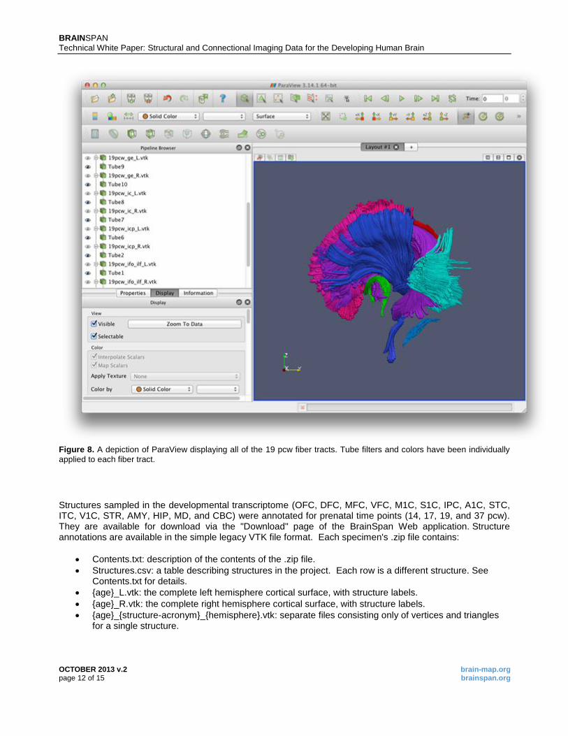
For complete cortical hemisphere surface files, structure vertex labels are listed at the end of the file in the "labels" field. This array is a list of integers in the same order as the vertex locations at the top of the file, each of which corresponds to a different structure. The labels correspond to the "label_id" column of "Structures.csv". All of these files can be opened directly in ParaView. To recolor the full cortical hemisphere surfaces by label:

1. Open the file 2. Click the "Apply" button in the "Properties" tab on the left 3. Open the "Display" tab. 4. Change the "Color by" field to "labels".

Figure 9 shows both hemispheres of a 14 pcw brain showing structure labels using the default color map.

Figure 9. Both hemispheres of a 14 pcw brain showing structure labels using the default color map.

BRAINSPAN



References

Benner et al. (2009) International Society for Magnetic Resonance Imaging in Medicine 17th Annual Meeting

Proceedings, Honolulu, Hawaii, 3535. Bloch F. (1946) Nuclear Induction. Physical Review 70:460-473. Fischl B, Salat DH, van der Kouwe AJW, Makris N, Ségonne F, and Dale AM. (2004) Sequence-Independent Segmentation of Magnetic Resonance Images. NeuroImage 23:S69-S84. Gilbert RJ and Napadow VJ. (2005) Three-dimensional muscular architecture of the human tongue determined in vivo with diffusion tensor magnetic resonance imaging. Dysphagia 20(1):1–7.

Gilbert RJ, Magnusson LH, Napadow VJ, Benner T, Wang R, Wedeen VJ. (2006) Mapping complex myoarchitecture in the bovine tongue with diffusion-spectrum magnetic resonance imaging. Biophysical J 91(3):1014–1022.

Gilbert RJ, Wedeen VJ, Magnusson LH, Benner T, Wang R, Dai G, Napadow VJ, Roche KK. (2006) Three-dimensional myoarchitecture of the bovine tongue demonstrated by diffusion spectrum magnetic resonance imaging with tractography. Anatomical Record 288(11):1173–1182.

Huang H, Zhang J, Wakana S, Zhang W, Ren T, Richards LJ, Yarowsky P, Donohue P, Graham E, van Zijl PC, Mori S. (2006) White and gray matter development in human fetal, newborn and pediatric brains. Neuroimage 33:27-38. Huang H, Xue R, Zhang J, Ren T, Richards LJ, Yarowsky P, Miller M-I, Mori S. (2009) Anatomical characterization of human fetal brain development with diffusion tensor MRI. J Neurosci. 29: 4263-4273. Huang H, Jeon T, Sedmak G, Pletikos M, Vasung L, Xu X, Yarowsky P, Richards L, Kostovic I, Sestan N, Mori S. (2012) Coupling diffusion imaging with histological and gene expression analysis to examine the dynamics of cortical areas across the fetal period of human brain development. Cerebral Cortex Aug 28 [Epub ahead of print].

Jenkinson M and Smith SM. (2001) A global optimisation method for robust affine registration of brain images. Medical Image Analysis 5(2):143–156.

Kang HJ, Kawasawa YI, Cheng F, Zhu Y, Xu X, Li M, Sousa AMM, Pletikos M, Meyer KA, Sedmak G, Guennel T, Shin Y, Johnson MB, Krsnik Z, Mayer S, Fertuzinhos S, Umlauf S, Lisgo SN, Vortmeyer A, Weinberger DR, Mane S, Hyde TM, Huttner A, Reimers M, Kleinman JE, Šestan N. (2011) Spatio-temporal transcriptome of the human brain. Nature 478: 483-489.

Le Bihan D. (1988) Intravoxel incoherent motion imaging using steady-state free precession. Magn Reson Med 7(3):346–351.

Mori S, Crain BJ, Chacko VP, van Zijl PC. (1999) Three-dimensional tracking of axonal projections in the brain by magnetic resonance imaging. Ann Neurol 45(2):265–269.

Roemer PB, Edelstein WA, Hayes CE, Souza SP, Mueller OM. (1990) The NMR phased array. Magn Reson Med 16(2):192–225. Wakana S, Jiang H, Nagae-Poetscher LM, Van Zijl PC, Mori S. (2004) Fiber Tract-based Atlas of Human White Matter Anatomy. Radiology 230:77-87.

BRAINSPAN



Wakana S, Caprihan A, Panzenboeck MM, Fallon JH, Perry M, Gollub RL, Hua K, Zhang J, Jiang H, Dubey P, Blitz A, van Zijl PCM, Mori S. (2007) Reproducibility of quantitative tractography methods applied to cerebral white matter. NeuroImage 36:630-644. Wald LL, Wiggins GC, Potthast A, Wiggins CJ, Triantafyllou C. (2005) Design considerations and coil comparisons for 7 T brain imaging. Appl Magn Reson 29(1):19–37. Wang R and Wedeen VJ. (2007) International Society for Magnetic Resonance Imaging in Medicine 15

th

Annual Meeting Proceedings, Berlin, 3720. Wedeen VJ, Hagmann P, Tseng WY, Reese TG, Weisskoff RM. (2005) Mapping complex tissue architecture with diffusion spectrum magnetic resonance imaging. Magn Reson Med 54(6):1377–1386.

Weiss S, Jaermann T, Schmid P, Staempfli P, Boesiger P, Niederer P, Caduff R, Bajka M. (2006) Three-dimensional fiber architecture of the nonpregnant human uterus determined ex vivo using magnetic resonance diffusion tensor imaging. Anat Rec A Discov Mol Cell Evol Biol 288(1):84–90. Wiggins GC, Polimeni JR, Potthast A, Schmitt M, Alagappan V, Wald LL. (2009) 96-Channel receive-only head coil for 3 Tesla: design optimization and evaluation. Magn Reson Med 62(3):754–62. Wright SM and Wald LL. (1997) Theory and application of array coils in MR spectroscopy. NMR Biomed 10(8):394–410. Zaraiskaya T, Kumbhare D, Noseworthy MD. (2006) Diffusion tensor imaging in evaluation of human skeletal muscle injury. J Magn Reson Imaging 24(2):402–408.

Documents

TECHNICAL WHITE PAPER: STRUCTURAL & …