Technical University of Munich Parametric Model Order

Chair of Automatic ControlDepartment of Mechanical EngineeringTechnical University of Munich

Maria Cruz Varona

Chair of Automatic Control

Department of Mechanical Engineering

Technical University of Munich

Model Order Reduction Summer School

September 24th 2019

Parametric Model Order Reduction: An Introduction

?

Reduced model for

query point pint

2

Linear Model Order Reduction

3

Projective Non-Parametric MOR

Linear time-invariant (LTI) system

Reduced order model (ROM)

MOR

Projection

4

1. Modal Reduction (modalMOR)

• Preservation of dominant eigenmodes

• Frequently used in structural dynamics / second order systems

2. Truncated Balanced Realization (TBR) / Balanced Truncation (BT)

• Retention of state-space directions with highest energy transfer

• Requires solution of Lyapunov equations, i.e. linear matrix equations (LMEs)

• Applicable for medium-scale models:

3. Rational Krylov subspaces (RK)

• “Moment Matching”: matching some Taylor-series coefficients of the transfer function

• Requires solution of linear systems of equations (LSEs) – applicable for

• Also employed for: approximate solution of eigenvalue problems, LSEs, LMEs,…

4. Iterative Rational Krylov algorithm (IRKA)

• H2-optimal reduction

• Adaptive choice of Krylov reduction parameters (e.g. shifts)

Linear MOR methods – Overview

5

Goal: Preserve state-space directions with highest enery transfer

Truncated Balanced Realization (TBR)

Controllability and Observability Gramians:

Procedure:

Energy interpretation:

1 Balancing step: Compute balanced realization, where

2 Truncation step:

Lyapunov equations:

6

Moments of a transfer function

Rational Interpolation by Krylov subspaces

: interpolation point (shift)

: i-th moment around

Bases for input and output Krylov-subspaces:

Moments from full and reduced order model around certain shifts match!

100

101

102

103

-100

-90

-80

-70

-60

-50

-40

Magnit

ude

/dB

Frequency / rad/ sec

original

(Multi)-Moment Matching by Rational Krylov (RK) subspaces

7

Balanced Truncation (BT)

Comparison: BT vs. Krylov subspaces

Rational Krylov (RK) subspaces

+ stability preservation

+ automatable

+ error bound (a priori)

+ numerically efficient

+ n ≈ 106

+ H2 -optimal (IRKA)

+ many degrees of freedom

computing-intensive

storage-intensive

n < 5000

many degrees of freedom

stability gen. not preserved

no error bounds

Numerically efficient solution of large-

scale Lyapunov equations

Krylov-based Low-Rank Approximation

• ADI (Alternating Directions Implicit)

• RKSM (Rational Krylov Subspace

Method)

Adaptive choice of reduction parameters

• Reduced order

• Interpolation data (shifts, etc.)

Stability preservation

Numerically efficient computation of

rigorous error bounds

Subject of research Subject of research

8

Parametric Model Order Reduction

9

Large-scale parametric model

Parametric Model Order Reduction (pMOR)

Flow sensing anemometer Timoshenko beam Microthruster unit

pMOR

Reduced order parametric model

• Linear dynamic systems with design parameters (e.g. material / geometry parameters,…)

• Goal: numerically efficient reduction with preservation of the parameter dependency

variation of the parameters in the ROM without having to repeat the reduction every time!

10

Projective Parametric MOR

High computational effort and

storage requirement needed for

simulation, optimization and control

Linear parametric system

Reduced parametric system

pMOR

11

Overview pMOR approaches

Common subspaces

for all

Individual subspaces

for local systems at

Global approaches Local approaches

Interpolation of transfer functions

[Baur ’09]

Interpolation of subspaces

[Amsallem ’08]

Interpolation of reduced matrices

[Eid ’09, Panzer ’10, Amsallem ’11]

Multi-Parameter Moment Matching

[Weile ’99, Daniel ’04]

Curse of dimensionality

Explicit parameter dependency requi.

Concatenation of local bases

[Leung ’05, Li ’05, Baur et al. ’11]

Affine parameter dependency required

Concatenation of the local bases

Computation of

using BT, RK, IRKA or POD

Reduced order:

Error bounds and stability

Local reduction using BT

Reduced order:

Interpolation of the reduction bases

Reduced order:

No explicit or affine parameter

dependency required

Reduced order:

Moment Matching w.r.t. and

12

(Weighted) concatenation of bases

• (Weighted) concatenation of local bases:

• Singular Value Decomposition:

• Reduction basis for new query point:

Concatenation of bases

(Weighted) concatenation of snapshots

Concatenation of snapshots is suitable, when the local bases

are calculated via an SVD-based technique like POD:

• (Weighted) concatenation of snapshots:

• Singular Value Decomposition:

• Reduction basis for new query point:

13

Interpolation of local bases is suitable for linear and nonlinear MOR!

Starting point: Local bases at parameter sample points

Procedure:

1. Choose a local basis for the reference subspace

2. Mapping of all subspaces onto the tangent space

using the logarithmic map:

3. Interpolation in the tangent space:

4. Backmapping of the interpolated subspace onto the manifold

using the exponential map:

Interpolation of subspaces[Amsallem et al. ’08]

Interpolation of reduced matrices:pMOR by Matrix Interpolation

14

15

pMOR by Matrix Interpolation – Main Idea

Model at Model at

Reduced model at Reduced model at

Model at

Reduced model at

Interpolation of

reduced matrices

Reduced model at from reduced

models at sample points &

?

16

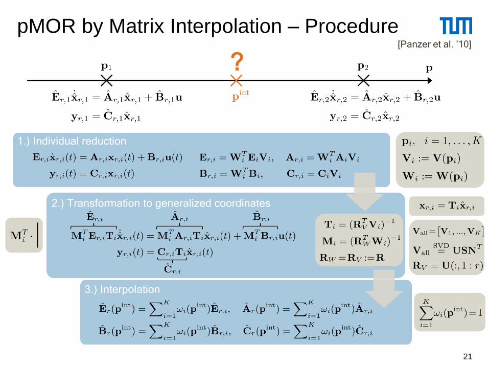
pMOR by Matrix Interpolation – Procedure

1.) Individual reduction

?

direct interpolation

not meaningful

[Panzer et al. ’10]

17


Choice of

?


2.) Transformation to generalized coordinates

?

How do we choose ?

Goal: Adjustment of the local bases to

, in order to make the gen.

coordinates compatible w.r.t. a

reference subspace .

Choice of

?

High

correlation

:


18


Choice of

?



?

Choice of

?

How do we choose ?

Goal: Adjustment of the local bases to

, in order to describe

the local reduced models w.r.t. the

same reference basis .

High

correlation

:

Analogous

to or


19





?

20





?

21




3.) Interpolation


?

22

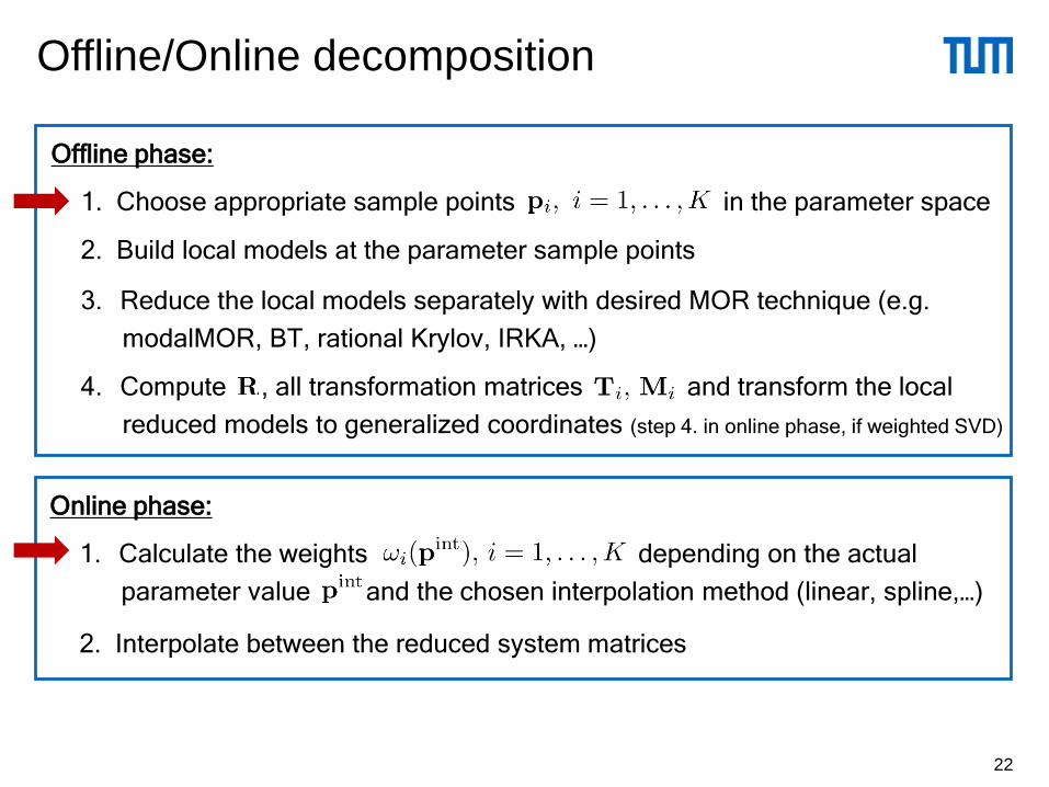
Offline/Online decomposition

Offline phase:

1. Choose appropriate sample points in the parameter space

2. Build local models at the parameter sample points

3. Reduce the local models separately with desired MOR technique (e.g.

modalMOR, BT, rational Krylov, IRKA, …)

4. Compute , all transformation matrices and transform the local

reduced models to generalized coordinates (step 4. in online phase, if weighted SVD)

Online phase:

1. Calculate the weights depending on the actual

parameter value and the chosen interpolation method (linear, spline,…)

2. Interpolate between the reduced system matrices

Sampling of the parameter space

Interpolation method (weighting functions)

23

24

Choice of parameter sample points is a critical question, specially in high-dimensional spaces!

Small number of parameters (d < 3)

• Full grid-based sampling or Latin hypercube sampling: Structured/uniform sampling,

random sampling, logarithmic sampling

• Moderate/high number of samples generated that covers the parameter space

Moderate number of parameters (3 ≤ d ≤ 10)

• In this case, full grid sampling quickly becomes expensive (curse of dimensionality)

• Latin hypercube sampling remains tractable

• Non-uniform sampling, sparse grid sampling

Large number of parameters (d > 10)

• Difficult to balance: number of sample points vs. coverage of the parameter space

• Problem-aware, adaptive sampling schemes required!

• Adaptive greedy search, sensitivity analysis using Taylor series, subspace angles, etc…

Sampling methods – Overview[Benner et al. ’15]

25

Adaptive Sampling

Requirements:

• Parametric space should be adequately

sampled

• Avoid undersampling and oversampling

• More parameter samples should be placed

in highly sensitive zones

Uniform Sampling:

Adaptive Sampling:Quantification of parametric sensitivity:

• System-theoretic measure that quantifies

the parametric sensitivity is needed in order

to guide the adaptive refinement

• Adaptive sampling using angle between

subspaces

• and are orthonormal bases for the

subspaces and

• The largest angle between the subspaces

can be determined by

: smallest singular value of

26

Concept of subspace angles:

Adaptive Sampling via subspace angles

Usage for adaptive grid refinement:

• The larger the subspace angle, the more

different are the projection matrices, and thus:

the higher the parametric sensitivity

and the more sample points can be

introduced in the respective sub-span

27

Automatic Adaptive Sampling: Pseudo-Code

1) Input

2) Divide the entire parameter range into a uniform grid,

calling it

3) While all do

a) Calculate the projection matrices

corresponding to each of these values

b) Compute subspace angles

between these ´s, each taken pairwise

c) Calculate

d) Divide the interval between and into further

intervals. Likewise, do the same for all the other

intervals.

e) Obtain new grid points , whereas

End While

Next iteration: local reduction,

etc. only at points that got

added in the last while-loop

iteration (efficient!)

theta(i) =

subspace(Vp{i},Vp{i+1})

Quantitative indicator of how

many pieces each parameter

interval is to be further broken

Local reduction at sample

points possible using any

preferred MOR technique

Stopping criterion:

1. All ratios are equal to 1

2. Specified maximum number

2. of samples points reached

[Cruz et al. ’17]

28

For the weighting or the interpolation, appropriate weighting functions should be selected!

Basically, any multivariate interpolation method could be used for this purpose:

• Polynomial interpolation (Lagrange polynomials)

• Piecewise linear interpolation

• Piecewise polynomial interpolation

(e.g. bi-/trilinear, cubic (splines), …)

• Radial basis functions (RBF)

• Kriging interpolation (Gaussian regression)

• Inverse distance weighting (IDW) based

on nearest-neighbor interpolation

• Sparse grid interpolation

Interpolation method – Weighting functions

1 1.5 2 2.5 3 3.5 4 4.5 5 5.5 6-0.4

-0.2

0

0.2

0.4

0.6

0.8

1

1 1.5 2 2.5 3 3.5 4 4.5 5 5.5 6-0.4

-0.2

0

0.2

0.4

0.6

0.8

1

[Benner et al. ’15]

pMOR Software

29

Chair of Automatic ControlDepartment of Mechanical EngineeringTechnical University of Munich

Toolbox – Analysis and Reduction of

Parametric Models in

Different parametric reduction methods

available (offline- & online-phase)

localReduction & adaptiveSampling

as core functions

Definition of parametric sparse state-

space models

Manipulation of psss-class objects

Compatible with the sss & sssMOR

toolboxes

psys = psss(func,userData,names)

psys = loadFemBeam3D(Opts)

psys = loadAnemometer3parameter

psys = fixParameter(psys,2,1.7)

psys = unfixParameter(psys,3)

param = [p1, p2, p3, p4]

sys = psys(param)

bode(psys,param); step(sys);

psysr = matrInterpOffline

(psys,param,r,Opts);

psysr = globalPmorOffline

(psys,param,r,Opts)

sysr = psysr(pQuery)

www.rt.mw.tum.de/?morlab www.rt.mw.tum.de/?psssmor

[sysrp,Vp,Wp] =

localReduction(psys,param,r,Opts)

paramRef =

adaptiveSampling(psys,param,r)

http://www.rt.mw.tum.de/?morlab

http://www.rt.mw.tum.de/?psssmor

Numerical Examples

pMOR in Applications

31

32

Numerical example: Beam model

Parameter: Length L

Thickness and width: 10 mm

Young Modulus: 2.105 Pa.

Damping: Proportional/Rayleigh

Order of the original system: 720

Order of the reduced system: 5

4 local models; Weights: Lagrange interp.

s0: ICOP (Eid2009);

Force

33

Numerical example: Solar panel model

Order of the original system: 5892

Order of the reduced system: 60

2 local models; Weights: Linear interpolation

Parameter: Thickness t of the panel

(varies between 0.25 and 0.5 mm)

www.orbital.com

34

• Finite element 3D model of a Timoshenko beam

• Parameter is the length of the beam:

• One-sided Krylov reduction with shifts at

• chosen

Numerical example: Timoshenko Beam[Cruz et al. ’17]

35

Initial uniform grid with

Numerical example: Timoshenko Beam

Final refined grid with

Adaptive S

am

plin

g S

chem

e

Interpolation point

between ROM 3 & ROM 4

[Cruz et al. ’17]

36

Numerical results – Direct vs. Interpolated ROM

FOM size n = 240, ROMs size r = 17 FOM size n = 2400, ROMs size r = 25

Two errors: model reduction error + interpolation error

[Cruz et al. ’17]

With MatrInterp: no need to reduce the model for every new parameter value

37

Numerical results – Initial vs. Final Grid

ROMs calculated with the final grid yield better approximations

FOM size n = 2400, ROMs size r = 25FOM size n = 240, ROMs size r = 17

[Cruz et al. ’17]

38

Numerical results – Initial vs. Final Grid

Relative H2 error between FOMs and

interpolated ROMs for different parameter

values and grids: FOM size n = 240, ROM

size r = 17

• Quantitative evaluation of the

approximation

• Relative H2 error for nP=100 different

query points

• Errors particularly small in the

proximity of the sample points

• Final grid yields smaller errors for

smaller beam lengths due to the

adaptive refinement in this region

[Cruz et al. ’17]

39

pMOR in Applications

Off-line applications:

• Efficient numerical simulation – “solves in seconds vs. hours”

• Design optimization – analysis for different parameters and “what if” scenarios

• Computer-aided failure mode and effects analysis (FMEA) – validation

On-line applications:

• Parameter estimation, Uncertainty Quantification

• Inverse problems, Real-time optimization

• Digital Twin, Predictive Maintenance

Physical domains:

mechanical, electrical, thermal, fluid, acoustics, electromagnetism, …

Application areas:

CSD, CFD, FSI, EMBS, MEMS, crash simulation, vibroacoustics, civil & geo, biomedical, …

40

[Baur et al. ’16] U. Baur, P. Benner, B. Haasdonk, C. Himpe, I. Martini and M. Ohlberger. Comparison of methods for

parametric model order reduction of time-dependent problems.

pMOR in Applications – Some success stories

[Pfaller et al. ’19] M. R. Pfaller, M. Cruz Varona, J. Lang, C. Bertoglio and W. A. Wall. Parametric model order reduction

and its application to inverse analysis of large nonlinear coupled cardiac problems. (on arxiv)

41

Summary & Outlook

References

42

Takehome Messages:

• Large, parametric FEM/FVM models (linear/nonlinear) arise in many technical applications!

• Parametric MOR (pMOR) is indispensable to reduce the computational effort!

• Global and local pMOR approaches exist: e.g. concatenation of bases, interpolation of

bases and matrix interpolation

• Offline/online decomposition of the methods

• Efficient sampling of the parameter space is crucial, especially for many parameters (d>10)

• Different interpolation methods and weighting functions available (linear, splines, RBF, …)

• pROMs can be applied for an efficient design optimization, inverse analysis, uncertainty

quantification, etc.

Challenges / Outlook:

• High-dimensional parameter spaces:

Adaptive sampling schemes

Avoiding the curse of dimensionality (tensor techniques!?)

• pMOR for systems with time-dependent parameters: p(t)MOR

Summary & Outlook

43

References (I)

[Amsallem ’08] D. Amsallem and C. Farhat. An interpolation method for adapting reduced-order models and application

to aeroelasticity. AIAA Journal, 46(7):1803-1813, 2008.

[Amsallem ’11] D. Amsallem and C. Farhat. An online method for interpolating linear parametric reduced-order models.

SIAM Journal on Scientific Computing, 33(5):2169-2198, 2011.

[Baur ’09] U. Baur and P. Benner. Model reduction for parametric systems using balanced truncation and

interpolation. at-Automatisierungstechnik, 57(8):411-419, 2009.

[Baur et al. ’11] U. Baur, C. Beattie, P. Benner and S. Gugercin. Interpolatory projection methods for parameterized

model reduction. SIAM Journal on Scientific Computing, 33(5):2489-2518, 2011.

[Baur et al. ’16] U. Baur, P. Benner, B. Haasdonk, C. Himpe, I. Martini and M. Ohlberger. Comparison of methods for

parametric model order reduction of time-dependent problems. Model reduction and approximation:

Theory and Algorithms, SIAM, Chapter 9, 377-407, 2016.

[Benner et al. ’15] P. Benner, S. Gugercin and K. Willcox. A survey of projection-based model reduction methods for

parametric dynamical systems. SIAM Review, 55(4):483-531, 2015.

[Cruz et al. ’17] M. Cruz Varona, M. Nabi and B. Lohmann. Automatic Adaptive Sampling in Parametric Model Order

Reduction by Matrix Interpolation. In: IEEE Advanced Intelligent Mechatronics (AIM), 472-477, 2017.

[Geuss et al. ’13] M. Geuss, H. Panzer and B. Lohmann. On parametric model order reduction by matrix interpolation.

In: IEEE European Control Conference (ECC), 3433-3438, 2013.

[Geuss et al. ’14a] M. Geuss, H. Panzer, T. Wolf and B. Lohmann. Stability preservation for parametric model order reduc-

tion by matrix interpolation. In: IEEE European Control Conference (ECC), 1098-1103, 2014.

44

References (II)

[Geuss et al. ’14b] M. Geuss, H. K. F. Panzer, I. D. Clifford and B. Lohmann. Parametric Model Order Reduction Using

Pseudoinverses for the Matrix Interpolation of Differently Sized Reduced Models. IFAC Proceedings

Volumes, 47(3):9468-9473, Elsevier, 2014.

[Geuss et al. ’15] M. Geuss, B. Lohmann, B. Peherstorfer and K. Willcox. A black-box method for parametric model order

reduction. In F. Breitenecker, A. Kugi and I. Troch (eds.), 8th MATHMOD, 127-128, 2015.

[Lohmann/Eid ’09] B. Lohmann and R. Eid. Efficient order reduction of parametric and nonlinear models by superposition of

locally reduced models. In Methoden und Anwendungen der Regelungstechnik – Erlangen-Münchener

Workshops 2007 und 2008, 2009.

[Panzer et al. ’09] H. Panzer, J. Hubele, R. Eid and B. Lohmann. Generating a parametric finite element model of a 3D

cantilever Timoshenko beam using MATLAB. Technical reports on automatic control (Vol. TRAC-4),

Lehrstuhl für Regelungstechnik, Technische Universität München, 2009.

[Panzer et al. ’10] H. Panzer, J. Mohring, R. Eid and B. Lohmann. Parametric model order reduction by matrix interpolation.

at-Automatisierungstechnik, 58(8):475-484, 2010.

[Pfaller et al. ’19] M. R. Pfaller, M. Cruz Varona, J. Lang, C. Bertoglio and W. A. Wall. Parametric model order reduction

and its application to inverse analysis of large nonlinear coupled cardiac problems. Submitted to

International Journal for Numerical Methods in Biomedical Engineering (https://arxiv.org/abs/1810.12033).

45

Backup

46

pMOR by Matrix Interpolation – Features

• No analytically expressed parameter-

dependency required

• Any desired MOR technique applicable

for the local reduction

• Offline/Online decomposition

• Reduced order independent of the

number of local models

Advantages Drawbacks

Properties:

• Local pMOR approach

• Analytical expression of the parameter-dependency in general not available

• Model only available at certain parameter sample points

Main idea:

• Choice of degrees of freedom

– Parameter sample points

– Interpolation method

• Stability preservation

• Error bounds

1 Individual reduction of each local model

2 Transformation of the local reduced models

3 Interpolation of the reduced matrices

47

Types of weighting functions / Interpolations

Explicit weights Implicit interpolation

Linear

interpolation

Nonlinear

interpolation

Matrices of the local reduced-order models

Spline

interpolation

Hermite

interpolation RBF

interpolation

48

Evaluation of the method according to different criteria

pMOR by Matrix Interpolation

Criterion Evaluation

Structure preservation

Reduced order

Storage effort

Computational cost

Offline/Online

decomposition

Stability preservation

Error bounds

49

Extensions for the Matrix Interpolation

Black-Box Methode

[Geuss et al. ’15]

• Ziel: Automatisierte pMOR-Methode

• Idee: Kreuzvalidierungsfehler für die

iterative Ermittlung von Stützstellen und

die optimale Wahl der Interpolations-

mannigfaltigkeit und Interpolations-

methode verwenden

Stabilitätserhaltung

[Geuss et al. ’14a]

• Interpolation (selbst stabiler) reduzierter

Modelle garantiert i.A. keine Stabilität

• Idee: Stabile reduzierte Modelle auf

dissipative Form bringen, damit ein

stabiles interpoliertes System resultiert

Lösung von Lyapunov-Gleichungen

Interpolation zwischen Modellen verschiedener reduzierter Ordnung

[Geuss et al. ’14b]

• Interpolation zwischen Modellen mit

unterschiedlicher reduzierter Ordnung

nicht möglich

• Idee: Basen auf dieselbe Größe

bringen durch die Berechnung von

mittels Pseudoinversen

Vereinheitlichendes Framework

[Geuss et al. ’13]

Framework mit folgenden Schritten:

1.) Wahl der Parameterstützstellen

2.) Reduktion der lokalen Modelle

3.) Anpassung der lokalen Basen

4.) Wahl der Interpolationsmannigfaltigkeit

5.) Wahl der Interpolationsmethode

Documents

Technical University of Munich Parametric Model Order