1

Technical Trading, Predictability and

Learning in Currency Markets

Valerio Potìa Richard M. Levich

b Pierpaolo Pattitoni

c

This version: 16 January 2012

This paper studies predictability of currency returns over time and the extent to which

it is captured by trading rules commonly used in currency markets. We consider the

strategies that an investor endowed with rational expectations could have pursued to

exploit out-of-sample currency predictability and generate abnormal returns. We find

a close relation between these strategies and indices that track popular technical

trading rules, namely moving average cross-over rules and the carry trade, implying

that the technical rules represent heuristics by which professional market participants

exploit currency mispricing. We find evidence that such mispricing reflects initially

wrong investors’ beliefs (wrong priors), but information is efficiently processed as it becomes available. Predictability is highest in the mid ’90, subsequently decreases

sharply, but increases again in the final part of the sample period, especially for the

Euro and other emerging currencies.

Key words: Foreign Exchange, Predictability, Market Efficiency

JEL Classification: F31

Contact details:

a

Valerio Potì, Room Q233, Dublin City University Business School and Cattolica

University S.C. at Piacenza, DCU Business School, Glasnevin, Dublin 9, Ireland;

Tel: 353-1-7005823, Fax: 353-1-7005446; Email: valerio.poti@dcu.ie. b

Richard M. Levich, New York University Stern School of Business, 44 West 4th

Street, New York, NY 10012-1126, USA. Tel: 212-998-0422, Fax: 212-995-4256; E-

mail: rlevich@stern.nyu.edu. c

Pierpaolo Pattitoni, Department of Management, University of Bologna, Bologna,

and the Rimini Centre for Economic Analysis (RCEA), Rimini, Italy; e-mail: pierpaolo.pattitoni@unibo.it; Tel: 39-051- 2098091; Fax: 39-051 -246411.

This paper is a heavily revised and expanded spin-off of a paper previously circulated

as “Predictability and Good Deals in Currency Markets”. The authors wish to thank

Chris Neely (Federal Reserve Bank of St. Louis), Ming-Yuan Leon Li (National

Cheng Kung University, Taiwan), Stephen Taylor (Lancaster University), Devraj

Basu (EDHEC), and discussants and participants to the INFINITI 2007 conference,

the EFM 2008 Symposium on Risk and Asset Management, the EFA 2008 meeting

and seminars at Lancaster University and Reading University ICMA Centre for

helpful comments and suggestions. Any remaining errors are the authors’ sole

responsibility.

2

Technical Trading, Predictability and

Learning in Currency Markets

This paper studies predictability of currency returns over time and the extent to which

it is captured by trading rules commonly used in currency markets. We consider the

strategies that an investor endowed with rational expectations could have pursued to

exploit out-of-sample currency predictability and generate abnormal returns. We find a close relation between these strategies and indices that track popular technical

trading rules, namely moving average cross-over rules and the carry trade, implying

that the technical rules represent heuristics by which professional market participants

exploit currency mispricing. We find evidence that such mispricing reflects initially

wrong investors’ beliefs (wrong priors), but information is efficiently processed as it

becomes available. Predictability is highest in the mid ’90, subsequently decreases

sharply, but increases again in the final part of the sample period, especially for the

Euro and other emerging currencies.

1. Introduction

In a literature that spans more than thirty years, various studies have reported that

filter and moving average crossover rules, as well as other technical trading rules,

including the carry trade, often result in statistically significant trading profits in

currency markets. Beginning with Dooley and Shafer (1976, 1984) and continuing

with Sweeney (1986), Levich and Thomas (1993), Neely, Weller and Dittmar (1997),

Chang and Osler (1999), LeBaron (1999), and Schulmeister (2006), among others,

this evidence suggests that currencies are predictable to an extent that casts doubts on

the efficient market hypothesis (henceforth, EMH). More recently, however, and

contrary to the bulk of these earlier findings, a number of authors, including Olson

(2004) and Pukthuanthong, Levich and Thomas (2007), find evidence of diminishing

profitability of currency trading over time. In a comprehensive re-evaluation of past

studies of filter and moving average (MA) rules, Neely, Weller and Ulrich (2009),

also find evidence of declining profitability. Based on these recent studies, it is

3

tempting to conclude that currency markets have become more efficient. Such

conclusion is, however, challenged by evidence that other strategies, such as trading

rules that exploit the so called “forward premium puzzle”, including until recently the

carry trade, continue to generate returns that appear to be large and relatively

uncorrelated with known risk factors. See, among others, Burnside et al. (2007),

Brunnermeir et al. (2008) and Jylha et al. (2010) as well as Neely, Weller and Ulrich

(2009), who also note that less popular and relatively more sophisticated strategies

continued to generate excess-profitability even as the profitability of the simpler and

more popular ones declined. Ultimately, these studies provide alternative and to some

extent conflicting views on the presence of mispricing in foreign exchange markets

and on whether currency trading is an economically useful endeavour.

In this paper, our aim is therefore twofold. On the one hand, we aim to shed light on

whether currencies and currency markets have indeed become less predictable and

more efficient, respectively. On the other hand, we seek to establish whether popular

currency strategies can be seen as trading heuristics employed by imperfectly rational

investors to exploit currency predictability in order to achieve rational or near-

rational trading outcomes, thereby eliminating over time currency mispricing. We

base our inferences on out-sample predictability. To this end, we compare and

contrast, on the one hand, stylized trading strategies that mimic popular currency

trading rules and, on the other hand, strategies that aim to generate the maximal

Sharpe ratio attainable by exploiting currency predictability. We refer to the former

as “technical trading rules” and to the latter as “rational trading rules”. The technical

rules are represented by the momentum strategy, tracked by the AFX Currency

4

Management index constructed by Lequeux and Acar (1998) by combining filter

moving average rules1 on the major currencies, and the carry trade, captured by the

HML Index of Lustig et al. (2011). The rational rules, instead, are based on a

predictive model that is meant to mimic the model that would have been used, at the

time of making the trading decision, by an investor endowed with rational

expectations (RE), as defined by Muth (1961) and later further formalized by Sargent

(1993). The study of in-sample predictability, which would also offer useful

indications, is left for parallel research work.

Our empirical results offer evidence of violations of the EMH at the beginning of the

sample period, i.e. in the early 90s, and in its final part, in coincidence with the

outbreak of the financial turbulence that characterized the period 2007-2010. This is

not only the case of emerging currencies, such as the Russian Rouble, the Brazilian

Real and the Polish Zloty, but also of the Euro. This suggests that the conclusion in

favour of vanishing profitability of technical trading rules, which has gained support

in recent years in the empirical literature, may be premature. More importantly, we

find that our rational trading rules are to a large extent tracked, over different

portions of the sample period, by the technical rules. This implies that technical

trading, far from being an irrational and wasteful endeavour, is a way for currency

portfolio managers to exploit, and hence eventually correct, mispricing relative to a

RE benchmark. It should be noticed that, because we use monthly data, our results

are robust to issues that crop up at higher-frequencies. For example, because of the

1 Menkhoff et al. (2011) point out that moving average rules do not capture in full the profitability that

can be generated by exploiting currency momentum but, as implicitly acknowledged by the same

authors, they are indeed representative of the strategies that have been traditionally employed by

currency managers and academics alike to do so.

5

low frequency of the strategies we consider, it is unlikely that non-proportional

transaction costs arising as a result of ‘price pressure’, e.g. Evans and Lyons (2002),

may play an important role. Overall, our evidence helps rationalize market

participants’ enduring tendency to engage in technical analysis and other active

currency management practices. As pointed out by Menkhoff and Taylor (2007),

currency traders exhibit an obstinate obsession for technical analysis, more so than

traders of other asset classes.

The remainder of our paper is structured as follows. In the next section, we outline

the relation between predictability and time-varying expected returns and illustrate

the rational trading rules which play a key role in our analysis. In Section 3, we

describe our dataset. In Section 4, 5 and 6, we present our empirical results on out-

sample predictability and market learning. In the final Section, we summarize our

main findings and offer conclusions.

2. Currency Predictability and Rational Trading Rules

We interpret an exchange rate as the price of a particular security, i.e. a default-free

interest-bearing deposit denominated in a foreign currency, with price and payoffs

expressed in terms of units of the domestic currency, i.e. the US Dollar, which in our

study acts as the numeraire. For ease of exposition, we will refer to such deposits as

the currencies in which they are denominated, e.g. the Canadian Dollar will be a unit

deposit denominated in such currency and funded in USD. We represent the data-

generating process (DGP) of currency excess-returns as follows:

6

1 1t t tr µ ε+ += + (1)

Here 1( | )t t tE r Iµ +≡ , tI is the information set at time t and 1+tε is a conditionally

zero-mean innovation, i.e. a (non-degenerate) random variable unpredictable with

respect to the information set t

I , i.e. �������� = 0, with finite but possibly time-

varying variance 2

,tεσ . Conditioning down, this implies���������� = ��������� =

0 ∀ �� ∈ ��. In this setup, the EMH boils down to the requirement that the expected

excess-return tµ equals the discount rate demanded by the marginal investor to hold

the asset, i.e. the currency. In the context of our tests of the weak-form EMH, t

I

includes the sigma-field generated by the past of 1tε +

, which belongs to the

information set �� available to the econometrician and we thus have �� = �, but it

may also include, in tests of the semi-strong and strong form EMH, other available

public and private information, in which case we might have �� ⊆ �, but this does not

need to concern us here as these forms of the EMH are outside the scope of the

present paper.

Our approach to testing the EMH in currency markets is based on the back-testing of

trading rules that seek to mimic the strategies that would have been followed by an

optimizing risk-averse currency trader endowed with RE. At any one time, the

simulated rational trading rule invests in the ith currency an amount of wealth

proportional to the expected excess-return and inversely to its conditional variance.

7

That is, the net amount of numeraire currency, i.e. the USD, invested in the ith

currency at any one time t under the rule is2

,

, 2

,

i t

i t

i t

wµ

λσ

= (2)

Here,

λ is an arbitrary but constant coefficient of proportionality. This strategy

combines a directional signal, i.e. the conditional mean ,i tµ , with a volatility filter,

i.e. 2

,i tσ . As shown by Cochrane (1999), it generates the maximal unconditional

Sharpe ratio (SR) attainable by exploiting the predictability of , 1i tr + , i.e. in our

context the excess-return on the ith currency. The strategy is very similar to the

“dynamic strategies” of Ferson and Siegel (2001). The only difference is that, in

Ferson and Siegel (2001, 2009), the ‘weights’ are also a function of the unconditional

SR and unconditional mean. For the one risky-asset case, the position taken in the i-

th currency at time t according to the Ferson and Siegel (2001, 2009) dynamic

strategy is

,

, 2 2

, ,

i t

i t

i t i t

wµ

λµ σ

=+

(3)

Here,

2 In-sample versions of these rules have been already used by Levich and Potì (2008).

8

( )* *

, ,*2

*2*2

*2

( ) ( )1

1

i t i tE r E rSR

SRSR

SR

λ = = +

+

and * *

,( )

i tSR SR r= is the maximal SR attainable by exploiting the predictability of the

ith currency and therefore the unconditional SR of the corresponding rational trading

rule. Whether we use the weights in (2) or in (3), the time t + 1 excess-return on the

resulting strategy is

*

, 1 , , 1i t i t i tr w r+ +=

(4)

To gain power against the market efficiency null, we also consider ‘average’

strategies consisting of investing in the rational trading rule for each currency i a

fraction iω of one’s portfolio. Denoting by n the number of currencies in which such

strategy invests at time t, it will have return

*

, 1 , , 1

1

n

avg t i i t i t

i

r w rω+ +=

=∑ (5)

To test the restriction ��������� = 0 ∀ �� ∈ ��, we (a) use maximum likelihood (ML)

to estimate a reduced-form representation of the DGP in (1), (b) use these estimate to

form forecasts of (excess-)retuns and their volatility, (c) use these forecasts in a

simulated rational trading rule defined by either (2) or (3) and, lastly, (d) test whether

the strategy offers abnormal return by testing for ‘alphas’ relative to a kernel 1+tm that

9

prices the traded assets. We adopt the usual linear functional specification for the

kernel, i.e.

1 1 'tm f b+ = + (6)

Here, f is a vector of factors and b is a conformable vector of parameters, with

elements that represent the negative of the associated factor risk prices. In (6), the

mean of the kernel is 1 ( ) 'E f b+ . This is legitimate because, when pricing excess

returns, the mean of the kernel is essentially not identified and therefore can be set

arbitrarily.

Our reliance on trading rules based on ML estimates of the DGP overcomes, at least

to some extent, a number of crucial shortcomings of prior tests of the weak-form

EMH. Our approach, in fact, does not require that the econometrician be able to

identify all trading strategies that rational investors could have possibly devised to

exploit episodes of currency mispricing (ML will do this for the econometrician, as

long as the model parameterization encompasses the DGP). This is instead an

implicit assumption of studies that attempt to make inferences on market efficiency

by testing for abnormal profitability of select technical trading rules. Because the

econometrician necessarily works with only a subset of available information and is

arguably not endowed with as much rationality as experienced traders (as suggested

by the say “if you are so smart why aren’t you rich”), and hence can identify at best

only a subset of possible trading strategies, findings in support of efficiency based on

this methodology may be suspect. On this, see also Griffin et al. (2010).

10

The usual remedy to this ill may be worse than the cure, as to gain power researchers

typically engage in a search over a wide range of strategies. There are two problems

with this approach, as noted in the seminal work of White (2000). First, by searching

long enough for a profitable rule, the analyst will sooner or later find one that, in a

simulated out-of-sample exercise, turns out to be profitable (“luck”). Second, with

the benefit of hindsight, the strategies in the search set may be known to have been

successful over the study period. Hence, inferences about genuine excess-

profitability might be misguided. Bajgrowicz and Scaillet (2012), applying the False

Discovery Rate (FDR) technique to the analysis of the out-of-sample performance of

equity technical trading rules, show that this is indeed the case. Our approach is

immune to such problems because, in using ML estimates of the DGP to generate our

out-of-sample forecasts, we simply impose the RE null with respect to the sigma

field generated by the past of the currency return process. That is, we are simply

replicating what a rational analyst, who has attended an undergraduate time series

econometric course, would do to identify and exploit predictability, if asked by the

currency manager (his boss) to do so. This analyst may be straight out of college and

not only have no access to private information but also (very realistically!) he may

not know too well sophisticated models of exchange rates. Our approach, in fact,

does not even require that the econometrician be able to identify and accurately

measure economic fundamentals. Given the profession’s imperfect understanding of

the exchange rate determination mechanism, this is another important advantage of

our approach. Since our out-of-sample tests are based on forecasts that exploit only

information contained in past prices (i.e. currency returns), however, they can only be

11

used to make inferences on the EMH in its weak form. Also, echoing remarks made

by Griffin et al (2010), they can detect mispricing only to the extent that exchange

rates do eventually revert to their RE fundamental valuation, and that they do so not

too slowly before the end of the sample period.

3. Data

Our dataset includes prices in US Dollars (USD) of the most liquid front-month

currency futures contracts over the period 1988-2010 traded at the Chicago

Mercantile Exchange (CME). These include the futures on the Australian and

Canadian Dollar, the Japanese Yen, the British Pound, the Swiss Franc, the Deutsche

Mark/Euro (we combine data on the Deutsche Mark futures before the introduction

of the Euro in 1999 and on the latter after its launch), the Norwegian Krone, the

Brazilian Real, the Polish Zloty, the South African Rand, the Russian Ruble and the

Turkish Lira. The futures prices are ‘chained’ to ensure comparability over time.

Also, to gain power against the EMH and extend the sample period, we broaden the

set of test asset payoffs by including currency portfolios considered by Lustig et al

(2008, 2011), constructed by sorting stocks according to the level of their interest

rates, and rebalanced yearly. These are the same portfolios used by Lustig et al

(2008, 2011) to construct HMLFX. The advantage of using portfolios of currencies

rather than the individual currencies is reduced sampling error, much in the same way

as when equity pricing models are tested on portfolios of stocks sorted along various

dimensions, rather than on individual stocks. In (6), remaining consistent with the

perspective of the American marginal investor, we use the time series of excess-

12

returns on the market, size and book-to market portfolios3 of US stocks that mimic

the Fama and French (1993) factors.

4. Performance of Predictability-Based Strategies

We first construct ‘baseline’ rational trading rules (excess-)returns using (2) in (4)

and (5). The inputs are monthly out-of-sample forecasts of excess-returns and

volatility generated using 5-year rolling windows of currency data. As a reduced

form representation of the excess-return DGP, we employ the following ARMA(p,q)

augmented by a GARCH(1,1) variance equation:

rt = const. + b1rt-1 + ..... + bprt-p + c1ut-1 + ..... + cqut-q + ut (7)

This choice is motivated by the fact that any stationary process can be represented as

an ARMA(p,q) for a suitable choice of p and q. Relatively parsimonious ARIMA

models of exchange rates, and thus ARMA models of currency returns, have been

shown to capture substantial predictability, e.g. Taylor (1994). Of course, we could

have used more flexible and complex specifications to gain power against the null of

no (excess-)predictability, but we would have left the door open to the danger of data

snooping. For comparison, however, we also use exponential smoothers that can be

seen as versions of the Kalman filter and therefore generalized versions of (7). To

keep our computational task manageable, however, we use in this case a constant

variance specification, treating the volatility input in (2) as an (arbitrary) constant. It

3 This data was downloaded from the website of Kenneth French, whose kindness we gratefully

acknowledge.

13

is very likely that our estimates of expected excess-returns contain a bias. Therefore,

when working with currency futures for which price data is available, we focus on

the information captured by the change in their forecast price and use

�

�

, 1

,

1 ,

( )ˆ 1

( )

t i t

i t

t i t

E S

E Sµ +

−

= − as our estimator of the expected currency futures excess return,

where �

, 1( )

t i tE S + denotes the one-step ahead forecast of the currency futures price

according to the estimated DGP reduced form representation. In this case, to generate

one-step forecasts of currency futures prices , 1i tS + , we use an ARIMA(p,q) model

with conditionally heteroskedastic errors, corresponding to the GARCH(1,1)-

augmented ARMA(p,q) of excess-returns in (7). When working with the interest rate-

sorted currency portfolios of Lustig et al. (2011), this approach is unpractical and, to

generate one-step ahead monthly forecasts of excess-returns and their volatility, we

use instead directly the ARMA(p,q) of excess-returns (i.e., rate of returns adjusted for

the net cost of carry) in (7) augmented by the GARCH(1,1) specification for the

variance process. To distinguish the rational rules based on currency futures data

from those based on the six interest rate-sorted portfolios constructed by Lustig et al

(2008, 2011), we denote the (excess-)return on former as ��,�∗ and the excess-return on

the latter as ��,�,�����∗ . In all cases, the predictive model that provides the reduced-

form representation of the DGP is estimated over 5-year rolling windows of monthly

currency data.

To estimate the predictive models we use Quasi Maximum Likelihood (QML). This

method is asymptotically equivalent to Maximum Likelihood (ML) in the presence of

possibly non-normally distributed errors, assuming stationarity and ergodicity of the

14

DGP. In large samples, it is thus consistent with the implications of the RE null under

relatively mild distributional assumptions. We use the ‘small sample’ version of the

AIC as the model selection criterion4, i.e. AICsmall = AIC + 2k (k + 1)/(l – k – 1),

where k = p + q. This version of the AIC was formulated by Sugiura (1978) and later

used by Hurvich and Tsai (1989). Just like the AIC, it adjusts the sample estimator of

twice the expected log-likelihood for its bias but, in doing so, it uses an expansion of

the bias of higher order than the one used by the AIC. It should be noticed that, in our

context, the search for the model with the optimal AIC does not imply a composite

hypothesis and hence does not require an analysis a la White (2000) or along the

lines of Bajgrowicz and Scailet (2012). In fact, our AIC-based search is simply a

consequence of imposing the EMH/RE null, which prescribes the maximization of

the expected (log-)likelihood. In carrying out our tests, we simply focus our attention

on the model that is picked by the AIC as the one with the largest (unbiased estimate

of the) expected log-likelihood and thus the most likely reduced form representation

of the DGP. In using the AIC as the model selection criterion, we allow for AR and

MA terms p and q of up to the fifth order.

The unrestricted baseline rational trading rule may exhibit substantial variation in the

allocation to each currency over time, entailing possibly substantial risk-taking. This

is not in principle a concern in tests of the EMH. In fact, in such tests, it is the

4 Unlike the Bayesian Information Criterion (AIC), the Akaike Information Criterion (AIC) is not consistent

(just like other popular criterions, such as the R2), in the sense of selecting the ‘true’ forecasting model with

the ‘correct’ list of regressors as the sample size increases without bounds. As also noted by Pesaran and

Timmermann (1995), however, the consistency property is not as important as it may appear at first when the ‘correct’ list of regressors is unknown and may be changing over time, as it is typically the case when

seeking to forecast asset returns. In such a context, as suggested by these authors, the ability to ex-post

select an explanatory equation “that could be viewed at the time as being a reasonable approximation to the

DGP” is of greater importance. The AIC, although statistically inconsistent, displays such ability, in that it has the property of yielding an approximate model and, as shown by Shibata (1976), strikes a good balance

between giving biased estimates when the order of the model is too low and the risk of increasing the

variance when too many regressors are included.

15

marginal positions that matter since optimizing investors are supposed to invest only

a marginal fraction of their wealth in each asset, in order to maximize diversification

benefits. Hence, since a marginal position is by definition infinitesimal, it does not

matter whether in the course of trading it needs to be incremented by any finite

though possibly very large factor. Nonetheless, to appreciate the effect of leverage on

the performance of the rational trading rules, we consider also the performance of

‘restricted’ rational trading rules, constructed under given restrictions on leverage.

We construct the strategies placing the restriction at different levels of leverage.

These include no leverage, denoted by lev = 0, and leverage equal to k times the

allocated risk capital, denoted by lev = k, where k is chosen so as to limit risk

exposure in line with typical risk-taking limits and stop-losses faced by traders.

Under these restriction, we have that ,i tw k≤ ∀ i and t.

Baseline rational trading rules

Table 1 reports descriptive statistics for the currency futures ‘baseline’ rational

trading rules, i.e. those obtained for each currency futures based on (2) and (4), for

their ‘equally weighted’ average strategy, with return as in (5) with 112iω = ∀ i,

where i refers to the i-th currency, for the technical trading rules, and for the Fama

and French factors. One noticeable fact is that, with some exceptions, the SRs of the

individual currencies rational trading rules are not particularly high. For example, the

SR of the average rational trading rule is 8 percent per month or 27 percent on an

annualized basis. Nonetheless, due to the low loadings (not reported to save space)

on the market and the other Fama and French factors, some of the strategies exhibit

16

statistically positive ‘alphas’. This is shown in Table 2 for the period 1997-2010,

which is the longest one for which we have enough data to estimate the out-of-

sample forecasting models for all currencies (which require 5 years of data each).

More importantly, the Table shows that predictability is more pronounced for

emerging currencies. Interestingly, it also suggests that the Euro should be perhaps

included among such emerging currencies, due to its high alpha. It is worth noticing

that the performance of the strategies based on the ARMA(p,q)+GARCH(1,1) model

is substantially better than those based on the exponential smoother, whereas the

latter is comparable to the performance of the strategies based on ARMA(p,q)

models with constant volatility (not reported to save space). This suggests that

modelling heteroskedasticity is important in capturing predictability and therefore,

from now on, we do not report results for the exponential smoother because we find

it computationally unduly demanding to augment it with a model of time-varying

conditional variance (we experienced substantial convergence and global

identification problems).

In Table 3, we report alphas and their associated t-tests, using both OLS and HAC

Newy-West (1987) standard errors, for a broader set of technical trading rules, and

both restricted and unrestricted average rational trading rules, which now also include

average rules based on the interest rate-sorted currency portfolios of Lustig et al.

(2011). In some cases, the leverage restriction considerably lowers the attainable

alpha. That is, the strongest evidence of EMH violations comes from strategies that

are difficult to implement in practice for the typical currency trader. Nonetheless,

they imply excess-volatility of exchange rates relative to a RE benchmark and

17

therefore, while difficult to risk-arbitrage, they imply allocative inefficiency and a

possible welfare loss that matters from a public policy perspective. Not surprisingly,

due to a diversification effect, the performance of the average rational rules based on

the interest-rate sorted currency portfolios is better than the one of the average

rational rule that exploits the predictability of the individual currencies, but

nevertheless they do not beat the technical trading rules.

Table 4 and 5, using for performance attribution the CAPM and the Fama and French

3-Factor model, respectively, offer a more detailed comparison of the strategies over

time. The Tables focus on the excess-performance of average unrestricted rational

rules that use different subsets of the currency futures, and compare them to the

excess-performance of the technical rules. Interestingly, Table 4 shows that, with the

exception of the final portion of the sample period, i.e. 2006-2010, excess-

predictability, as picked up by the rational rules, appears to be confined to emerging

currencies and the Euro. The AFX momentum strategy and the carry trade alternate

as sources of favourable abnormal performance over the periods 1996-2000 and

2001-2005, with the latter taking over from the former in the later period. The

rational rule picks up some marginally significant excess-predictability also in the

initial part of the sample period, i.e. 1992-1995. This pattern can be seen in Figure 1,

which plots the CAPM alphas for the average rational rules for the emerged and

emerging currencies. There is a marked ‘slump’ of alphas in the central period, about

2001-2007, essentially yet another manifestation of the phenomenon known as the

“great moderation”, preceded by relatively high excess-predictability in the first half

of the 90s (it should be kept in mind that the alphas are estimated over rolling

18

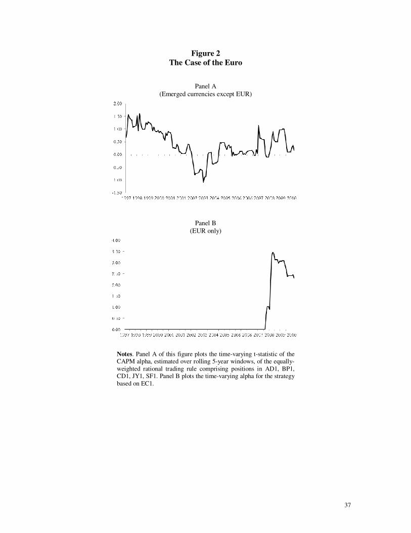
windows looking backwards 5 years) and followed by a spike after 2007. As shown

in Figure 2, however, the sudden rise of alpha of the emerged currencies rational rule

is largely explained by the surge of the alpha of the Euro strategy, suggesting again

that perhaps this currency should be treated as an emerging one, due to its relatively

recent introduction or the market learning that (has) had to take place about the

somewhat unusual institutional arrangements behind it. Table 5 offers similar

indications though, in this case, abnormal performance is confined to the Carry

Trade, in 2001-2005, and the average rational rule for the emerging currencies as

well as the EUR, in the final 2006-2010 period.

Optimal rational trading rules

To gain power against the EMH, we now turn to considering the ‘optimal’ trading

rules based on the Ferson and Siegel (2001, 2009) ‘weights’ in (3). The estimates of

the conditional moments in (3) are given, as before in (2), by their out-of-sample

forecasts. As for the unconditional moments, *

,( )

i tE r is simply the target excess-

return expected from the strategy and can be chosen arbitrarily whereas *2SR

requires careful modelling. In the out-of-sample context of our study, while we can

assume knowledge of unconditional moments thanks to RE, we need to be careful in

using their sample counterparts as their estimates. This, while consistent with the RE

null under the assumption that the DGP is stationary and ergotic, would entail a

testing strategy with an in-sample dimension.5 Nonetheless, we can usefully adapt the

Ferson and Siegel (2001, 2009) approach. To do so, we take RE to its extreme 5 There seem to be a strong prejudice in the profession against in-sample tests of predictability and

therefore we are threading carefully so as to avoid any suspect that our out-of-sample tests might have

suffered some in-sample ‘contamination’.

19

implications and assume that the investor knows the maximal SR attainable from

exploiting predictability and the sample SR, ex post, turns out what the investor

expected ex-ante. That is, we set *SR equal to the sample SR of the trading rule. The

problem, in this approach, is that we can only compute the sample SR after we have

constructed the weights and computed the strategy excess-returns, using (4). To solve

the circularity, we therefore compute the SR and weights iteratively, starting from an

initial guess for *2SR equal to 4.42 percent (i.e., the variance of the kernel assuming

a relative risk aversion of the marginal investor equal to 2.5 and a market volatility

equal to about 20 percent per annum and approximating the volatility of the kernel as

the product between relative risk aversion and market volatility). The ‘estimation’

converged to the desired weights and a monthly �*2

SR equal to 2.38 percent after just

three iterations.

The upshot of using (3) instead of (2) is that extreme weights are ‘automatically’

curbed, as explained by Ferson and Siegel (2001), so we do not have to impose

leverage limits in constructing the rules. For example, the weights of the rule with

expected (excess-return) equal to 10 bps per month never exceed one in absolute

value whereas those of the rule with expected (excess-return) equal to 50 bps per

month never exceed four in absolute value. In practice, this means that, by rationally

exploiting currency predictability, it is possible to maintain a position that yields 50

bps per month over the risk-free rate. The risk-free return would come from risk-free

bonds posted as collateral (assuming that one has collateral to post, something that in

the current ‘collateral crunch’ is not to be taken for granted!). Since the weight never

exceeds four in absolute value, the collateral posted would remain within a 25

20

percent margin of the exposure, something that is deemed acceptable by many

brokers, while the trading rule would provide the additional 50 bps per month.

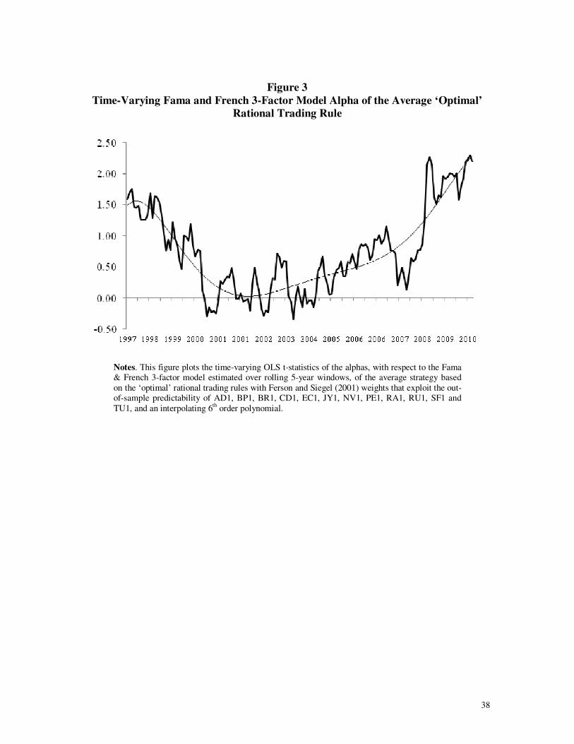
Furthermore, as shown in Figure 3, the rules have very rarely since 1997 experienced

significant losses. The figure plots the t-statistics of the rolling 5-year alphas (with

respect to the Fama and French 3-factor model) of the rules with expected (excess-

)return equal to 10 bps per month. The corresponding plot for the average rule with

expected (excess-)return equal to 50 bps per month is almost indistinguishable and is

not reported to save space. Similarly to the ‘baseline’ average rational rules, the

series undergoes two clearly distinct ‘trends’, i.e. a descending one in 1997-2003 and

an ascending one subsequently thereafter. The spike in the final part of the sample

period, however, is more pronounced and the performance after 2003 is also

generally better. On balance, this means that the optimal average rational rules are a

rather attractive proposition for the fully rational trader who, thanks to his RE

knowledge of unconditional moments, may be in a position to implement them.

In Table 6, we report the estimated alphas and factor loadings (with respect to the

Fama and French 3-factor model) of the optimal average rational rule based on the

predictability of the currency futures in our dataset and expected (excess-)return

equal to 10 bps per month. The noteworthy aspect is that, while the strategy does

significantly outperform the AFX and carry trade, as implied by its positive and

significant alpha, this is only down to the periods 1992-1995 and 2006-2010. In the

period 1996-2000, instead, the alpha of the rational trading rule is even negative and

in 2001-2005 it is positive but insignificant. Therefore, in the central part of the

sample period, the AFX and carry trade, i.e. the predictability-based strategies

21

resembling those followed by market practitioners, indeed span the rational trading

rules based on ML and optimal mean-variance optimizing portfolio formation. The

‘anomaly’ is the alpha, i.e. un-spanned performance, of the rational trading rule at the

beginning and at the end of the sample period, which points to inefficient currency

pricing during these periods.

5. Currency market learning tests

Both the technical and the rational rules exhibit positive and statistically significant

alphas over extended portions of the sample period. This is especially the case of the

levered and the ‘optimal’ rules. This implies that, at those times, the EMH was

violated resulting in currency pricing not in line with RE, at least from the point of

view of a representative investor who can take marginal positions in the strategies,

and therefore does not need to be concerned about possibly high leverage, and/or is

endowed with enough rationality to ‘know’ the unconditional SR of the strategies

rules, so that she can implement the ‘optimal’ rational rules. In constructing the rules,

we already controlled for transaction costs and, at the relatively low frequency of our

study (monthly), the impact of microstructure effect that are typically felt at higher

frequencies is likely limited, e.g. we can rule out price pressure effects on execution

prices since the trader has plenty of time to execute them (a month!) without moving

the market.

A possible explanation that is left to explore is learning. More specifically, the

positive performance of predictability-based strategies might reflect either

22

predictability induced by market learning, starting from possibly biased priors, or

outright inefficient processing of news. The first possibility is consistent, in the

language of Bossaerts (2004) and along the lines of Hansen (2007) and Hansen and

Sargent (2007), with efficient market learning (EML) whereas the second is not. To

test for violations of EML, we follow Bossaerts (2004) and construct ‘modified’ risk

adjusted-rates of returns, i.e.

1~

+tr ≡

1

1

~

~~

+

+ −

t

tt

p

pp (8)

where 1 0...t t t tp p m m m−≡ɶ is the ‘price’ of the strategy at time t deflated back to time t

= 0, with t = 1, 2, …, T – 1, where sm is the pricing kernel in t = s. The un-deflated

‘price’ s

p is computed by capitalizing an initial one USD investment (made at time

0) at the strategy rate of return, e.g. at the rate *

,i tr

for the rational trading rules for the

i-th currency, until time t. For the purpose of testing for inefficient learning against

the alternative represented by Bossaerts’ (2004) ELM, we interpret the strategy as a

strip of “winning” securities, i.e. securities that offer payoffs Tωɶ in T (capital

accumulation at the end of the sample period) that exceed a given threshold TV ,

which is possibly different across ‘securities’ but large enough to entail an ‘alpha’ of

the overall strategy as large as the one observed.

Under ELM, the market prior beliefs about such payoffs may be biased, i.e. the

market may initially underestimate the payoff unconditional probability, but market

beliefs are updated efficiently as new information becomes available, i.e. the

23

posterior converges to the unconditional probability at the rate predicted by efficient

Bayesian learning. The key result is that the modified returns in (8), as implied by

Bossaerts’ (2004) Theorem 3 for the case of the general “winning” limited-liability

security and under relatively mild technical assumptions6, are on average negative

when a representative investor, who employs Bayesian updating, uses the correct

likelihood in forming her beliefs about the predictive distribution of returns,

1( | ) 0t t T TE r Vω+ > ≤ɶ (9)

This inequality only requires that the Bayesian marginal investor uses the correct

likelihood function of the data given final payoffs at time T, not necessarily the

correct prior about the (deflated) payoff being above the given threshold TV . In

specifying the kernel, which is needed to deflate the payoffs, we face the difficulty

that we do not know it on a priori grounds. It is unclear how we could estimate the

kernel if we were to adopt a parametric specification because (9) does not represent a

traditional orthogonality condition, and therefore the standard empirical asset pricing

estimation and testing machinery is ill-equipped to handle it. As a way around this

difficulty, the deflation is conducted by specifying the pricing kernel as in the power-

CAPM, i.e. by setting

6 The two assumptions are that (a) the conditional expectation of the payoff outside of the “default

state” (i.e., the state that did not occur with the expected frequency in which the payoff comes in lower

than VT) is correct and (b) the market until time T never knows for sure that the default state occurs.

The first assumption is labelled by Bossaerts (2004) “Correct Conditional Expectation” (CCE), and

essentially amounts to imposing efficient learning, and the second one is labelled No Early Exclusion

Hypothesis (NEEH), which is highly reasonable in our context.

24

1

, , 1

1

1

RRA

t

f t m t

mr r

+

+

= + +

(10)

Here, ,f tr is the conditionally risk-free rate of interest, , 1m tr + is the market excess-

return and RRA is the coefficient of relative risk aversion of the marginal investor,

which we set equal, following Potì and Wang (2010), to either 2.5 or 5.0, i.e. RRAV =

2.5 and RRAV = 5. As argued by these authors, the first choice is consistent with the

classic two-moment CAPM whereas the second choice is consistent with 3 and

higher moment extensions of this model, along the lines of Kraus and Litzenberger’s

(1976) 3M-CAPM and Dittmar’s (2002) 4M-CAPM, as well as with the Fama and

French 3-Factor model and other specifications, such as habit formation models and

conditional models, that generate relatively large economy-wide maximal SRs. The

average modified risk-adjusted returns for a number of technical and rational trading

rules based on such deflation are reported in Table 7, together with t-statistics

constructed using OLS standard errors, for both the full sample periods for which

each strategy can be constructed and for the shorter sample period, from 1997 to

2010, for which data is available for all strategies. Under the EML null and the

inefficient market learning alternative, the reported t-statistics should be non-

positive. Equivalently, under the inefficient market learning null, the t-statistics are

positive. As shown in the Table, we can reject the latter null in one-sided tests at

conventional levels for most rules. The exceptions are the leveraged rational trading

rules and the optimal rational rules under RRAV = 2.5 in the shorter sample period,

i.e. in 1997-2010. For such rules, we cannot reject inefficient learning though the

statistics are not positive enough for us to reject ELM. On balance, these results

25

overwhelmingly support the view that currency markets are indeed efficient in

processing information as it becomes available, in spite of (unspecified) biases in

prior beliefs implied by the EMH violations, i.e. by the ‘alphas’ of the rational and

technical trading rules.

6. Currency trading and market learning

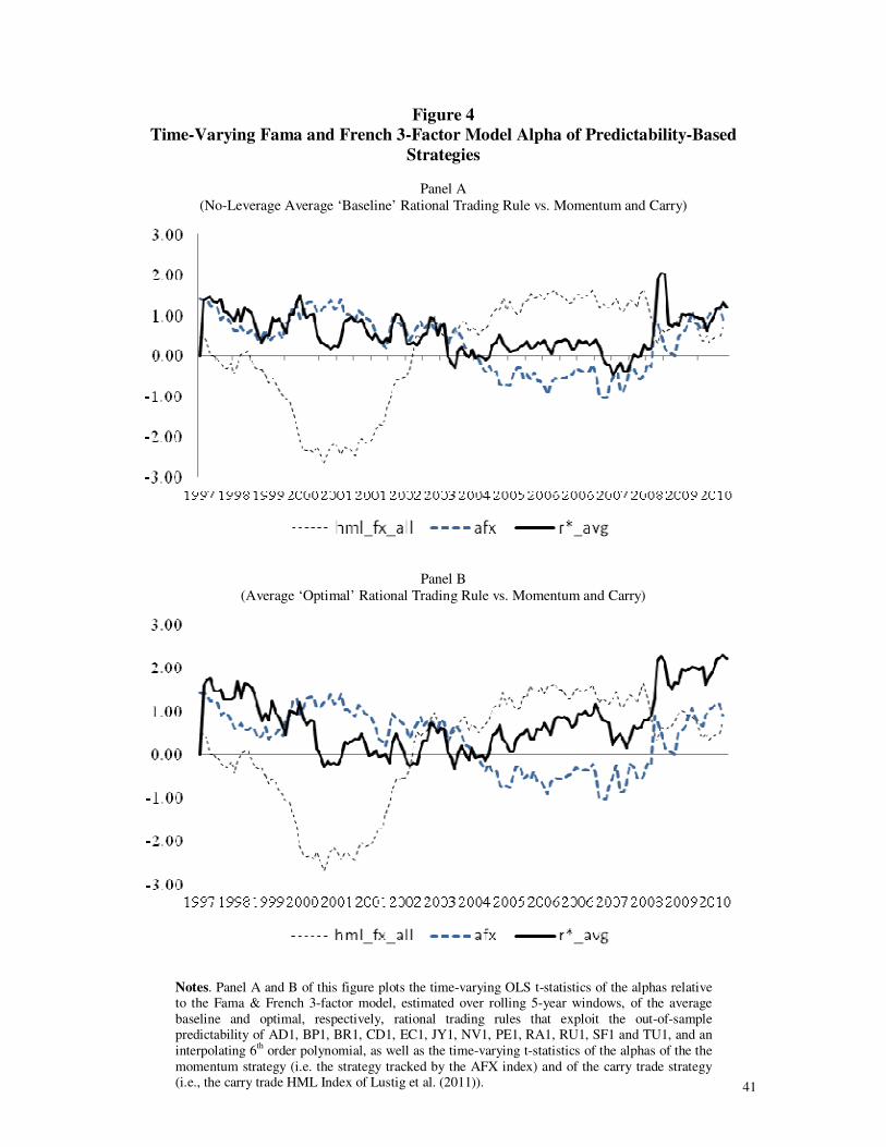
To appreciate how currency market efficiency evolves over time, in Panel A and B of

Figure 4, we plot the OLS t-statistics of the rolling alphas of the currency futures

average ‘baseline’ and ‘optimal’ rational rules with expected (excess-)return of 50

bps per month, as well as those of the momentum and carry trade technical rules. The

baseline rule is constructed under no-leverage restriction. They are similar in terms of

both their order of magnitude and pattern of variation over time, but the ‘optimal’

one tracks the carry trade more closely when the latter performs best. There is also in

both cases a striking overlap between the rational trading rule and the AFX index,

except during 2003-2007. The overlap is all the more remarkable when one considers

that the two strategies are based on a completely different construction methodology,

though they seek to capture the same source of predictability.

The AFX is a value-weighted index of simple moving average strategies, consisting

of buying or selling one unit of a given set of currencies based on signals generated

by the cross-over of the exchange rate with its moving averages of pre-specified

length, with weights that reflect the importance of each currency pair in world

currency trading. Therefore, it can be interpreted as the momentum rule followed by

26

the ‘representative’ currency manager. The rational trading rules, instead, are based

on the weights described in (2), which in principle can take any real value and reflect

a directional signal and volatility filter generated by a predictive model, i.e. the

ARMA(p,q) augmented by the GARCH(1,1), selected and estimated using ML, in an

effort to mimic RE. Moreover, the AFX index only takes positions in the main

currencies, i.e. DM/EUR, GBP, JPY and CHF, against the USD and each other,

whereas the average rational trading rule is based on a broader set of currencies that

include emerging ones. Nonetheless, the ‘baseline’ rational trading rule ‘beats’ the

AFX Currency Management index only during 2003-2007. During this time,

however, the rational rule is, in turn, beaten by the carry trade strategy, i.e. the

HMLFX in the figure. True, as shown in Table 6 and also in Panel B of the Figure,

the ‘optimal’ rational rule beats the AFX over much of the post-2003 period but, as

already noted, implementing this strategy requires ex-ante knowledge of its

unconditional SR. This might be too stringent a requirement in practice. Imperfectly

rational currency portfolio managers may well hold initially wrong priors and learn

the true unconditional SR of the rule only slowly. Therefore, if we postulate even

mild limits to investors’ rationality, and hence leave out rules that are ‘too’ rational,

we see that during our sample period there is always a strategy, out of those followed

by market practitioners and replicated in stylized manner by our technical trading

rules, that either closely matches or beats the rational ones. This suggests that the

technical trading rules have been used, at different points in time, as heuristics by

which a possibly imperfectly rational market practitioner have achieved an

essentially rational outcome, while likely economizing on scarce resources such as

managerial attention.

27

A crucial question is then whether market practitioners are able to decide when it is

the right time to switch technical trading strategy. There is no data on the ‘relative

usage’ of different technical rules over time but we can gauge their popularity by

measuring how frequently words associated to such strategies appear in the press. In

Panel A and B of Figure 5 we plot the usage over time of the phrases “carry trade” as

well as “filter rule” and filter rules”, respectively, in the book database searched by

Google Ngram Viewer7. The database includes more than 500 billion words (361

billion for the English language) from 5,195,769 digitized books, or about 4 percent

of all books ever published. Rather remarkably, the usage of the words “carry trade”

picks up in 2003, right when the usage of the words “filter rule” and/or “filter rules”,

by which professional currency managers commonly refer to momentum technical

rules of the type considered in this paper, declines. The books containing such words

are most likely professional publications or at least they are geared towards a public

of practitioners, since the privileged outlets for academic articles by financial

economists operating in English-speaking countries tend to be peer-reviewed

scientific journals. These trends, therefore, suggest that the world of currency

managers, or at least the publishers catering for their reading needs, turned its

attention away from filter rules and towards the carry trade precisely at the time when

the former were starting to under-perform both the latter and the rational trading

rules. Unfortunately, at the time of writing, the Google Ngram database only includes

words appeared in books published until the end of 2008 and therefore it is not

7 The link to the tool, with the search set on the words “filter rule” and “filter rules”, is:

http://books.google.com/ngrams/graph?content=filter+rule%2C+filter+rules&year_start=1997&year_

end=2008&corpus=0&smoothing=3

28

possible to establish whether the relative trend in the word usage reversed when the

carry trade turned unprofitable relative to the filter/momentum rules after 2008.

7. Conclusions and Final Remarks

In this paper, we assess the statistical and economic significance of predictability in

currency returns over the period 1971-2010. We find that predictability at times

violates RE restrictions, implying that currencies are mispriced relative to the RE

benchmark and violation of the EMH. Currency mispricing and currency market

inefficiency are not constant over time but their evolution does not fully conform to

the popular view that currency markets are becoming increasingly efficient over time.

While it is true that currency excess-predictability, and thus mispricing decreases in

the 90s, it does pick up again in recent times. This is especially the case of currencies

of emerging market economies, but not exclusively. In fact, the Euro, which is

relatively new as a currency but is in use in a highly developed economic area,

experienced the most dramatic surge in excess-predictability. We find, however, that

popular currency trading strategies represent simple and effective ways to capture the

bulk of such excess-predictability and that, in spite of the latter and the degree of

currency mispricing that it implies, currency market learning unfolds efficiently, that

is markets process new information efficiently as it becomes available though they

may misprice currencies due to initially wrong priors.

On the one hand, our results pose a stronger empirical challenge to established

models of rational exchange rate determination than previous ones in that they imply

29

that it might be premature to brush off excess-predictability as a temporary

phenomenon, largely disappearing or due to disappear shortly as soon as currency

markets will have completed their journey towards full efficiency. On the other hand,

and more importantly, our results suggest that technical trading rules are largely a

rational attempt by market participants to exploit predictability. That is, both the filter

strategies tracked by the AFX index and, subsequently, the carry trade have acted, at

different points in time, as ways in which speculators have attempted to exploit

currency market inefficiencies. This, in turn, helps answer the important question of

whether such strategies create or prick “bubbles” inherent in the episodes of

inefficient pricing. The evidence appears to suggest the latter, although more

investigation is required before a firmer conclusion can be reached.

It also remains to be established why they do not do so in a more direct way. In fact,

technical trading can be seen as a means to exploit excess-predictability without

having to first detect it. Therefore, if market participants were able to directly detect

mispricing through the currency market counterpart of ‘fundamental analysis’,

presumably they would not need to resort to technical trading. The question then is

what prevents currency market participants from identifying and exploiting currency

mispricing in a more direct way. Possible explanations might lie in both the rational

asset pricing domain, e.g. costs required to undertake the analysis and other frictions,

or in the behavioural domain, e.g. limits to rationality, or possibly somewhere in

between, for example the need to economize on scarce managerial attention as in the

model formulated by Bacchetta and van Wincoop (2010). Either way, a fruitful

30

direction for future research is to explore the role of technical trading rules as

heuristics deployed by market participants to supplement their pricing abilities.

31

Table 1

Descriptive statistics of predictability-based strategies returns

Obs Mean St. dev. SR SR ann. Skew. Kurtosi

s

Panel A (Rational trading rules)

AD1 212 0.54 8.34 0.06 0.22 -0.15

(0.648)

4.60

(0.000)

BP1 212 -0.14 3.52 -0.04 -0.14 1.00

(0.003)

4.75

(0.000)

CD1 212 0.02 6.80 0.00 0.01 1.22

(0.000)

8.44

(0.000)

JY1 212 0.07 5.31 0.01 0.04 -1.28

(0.000)

5.91

(0.000)

SF1 212 0.17 5.01 0.03 0.12 -1.44

(0.000)

9.25

(0.000)

EC1 85 1.60 17.37 0.09 0.32 2.02

(0.000)

11.13

(0.000)

NV1 97 0.43 8.07 0.05 0.18 -1.84

(0.000)

9.19

(0.000)

BR1 115 0.89 8.66 0.10 0.36 1.59

(0.000)

8.47

(0.000)

PE1 122 6.49 37.00 0.18 0.61 2.88

(0.000)

11.74

(0.000)

RA1 97 1.70 23.99 0.07 0.25 2.52

(0.000)

10.60

(0.000)

RU1 86 0.36 1.67 0.22 0.75 4.55

(0.000)

23.25

(0.000) TU1 180 -0.02 6.83 0.00 -0.01 -0.17

(0.000)

3.74

(0.000)

All (average) 212 1.01 13.14 0.08 0.27 2.70

(0.000)

14.50

(0.000)

Panel B (Other predictability-based strategies and risk factors)

AFX 212 0.18 1.76 0.10 0.36 2.035

(0.000)

6.83

(0.000)

HMLFX All 212 0.43 2.53 0.17 0.59 -0.91

(0.001)

0.54

(0.446)

HMLFX

Developed

212 0.19 3.08 0.06 0.22 -0.66

(0.0522)

1.09

(0.123)

Rm - Rf 212 0.45 4.54 0.10 0.34 -0.84

(0.013)

1.599

(0.024)

SMB 212 0.26 3.60 0.07 0.25 0.42

(0.218)

-0.27

(0.700)

HML 212 0.37 3.49 0.10 0.36 -0.50

(0.142)

1.78

(0.012)

Notes. This table reports descriptive statistics for returns on maximal SR-rational trading rules for each

currency and their average, in Panel A, and for other predictability-based strategies, i.e. the momentum strategy tracked by the AFX Currency Management index and the carry trade strategy tracked by the HML

Index of Lustig et al. (2011), as well as the Fama and French factors. The descriptive statistics are the

number of monthly observations, the percentage mean, standard deviation, SR (monthly and annualized),

skewness and kurtosis (together with their p-values under the null of no departure from normality).

32

Table 2

Out-Of-Sample Performance vs. Fama & French 3-Factor model of Rational Trading Rules

1997-2010

AD1 CD1 JY1 BP1 SF1 EUR NV1 BR1 PE1 RA1 RU1 TU1

ARIMA+GARCH

SR 22.42 0.82 4.34 -13.54 11.77 32.00 18.49 35.70 60.73 24.60 74.54 -1.22

α 0.96 -0.09 -0.01 0.16 -0.05 4.21 1.31 1.76 6.01 5.26 0.57 0.02

t-statistics 1.35* -0.15 -0.03 0.51 -0.11 1.80** 1.28* 1.74** 1.44* 1.74** 2.54** 0.04

p-value (0.089) (0.439) (0.490) (0.305) (0.458) (0.037) (0.100) (0.041) (0.076) (0.041) (0.006) (0.485)

ETS

SR 14.91 -11.37 3.51 19.36 -8.50 -11.94 3.31 23.73 42.34 -3.03 27.63 11.30

α 0.00 -0.00 -0.00 0.00 -0.00 0.00 0.00 0.00 0.01 0.01 0.03 0.00

t-statistics 1.51* -0.16 -0.10 2.17** -0.47 0.70 0.86 1.23* 2.04** 0.72 1.43* 0.12

p-value (0.066) (0.437) (0.461) (0.015) (0.320) (0.241) (0.195) (0.111) (0.021) (0.236) (0.078) (0.452)

Notes. This table reports, in the top panel, percentage alphas and annualized Sharpe Ratios of predictability-based maximal-SR strategies, as well as the t-statistics of the alphas and the corresponding p-values (in brackets). The hypothesized level of transaction costs is two basis points (i.e. 0.02 percent) per each way transaction and the predictive models are

ARMA(p,q) with p and q selected by the AIC estimated over rolling 5-year windows over the sample period 1992-2010. The data frequency of the underlying currency futures return

series is monthly. One and two asterisks draw attention to positive alpha significant at the 10 and 5 percent level, respectively.

33

Table 3

Out of Sample Performance of predictability-based strategies vs. Fama and French

3-Factor Model

alpha (perc.)

OLS s.e. (perc.)

OLS t-stat. HAC s.e. (perc.)

HAC t-stat.

1992-2010

Technical trading rules

HMLFX (developd) -0.02 0.20 -0.09 0.22 -0.08

HMLFX (all) 0.33 0.17 *1.94 0.17 *1.89

AFX 0.20 0.12 *1.65 0.09 *2.29

Rational trading rules

r*avg (all, lev. = unrestricted) 8.61 6.86 1.26 7.34 1.17

r*avg (all, lev. = 0) 0.10 0.06 *1.65 0.06 *1.71

r*avg (emer., lev. = unrestricted) 5.65 2.25 *2.51 3.37 *1.68

r*avg (emer., lev. = 0) 0.08 0.06 1.34 0.06 1.42

Rational trading rules –

Lustig et al. (2011) portfolios

r*avg, carry (all, lev. = 10) 6.76 3.29 *2.05 3.18 *2.12

r*avg, carry (all, lev. = 4) 2.76 1.43 *1.93 1.40 *1.97

r*avg, carry (all, lev. = 0) 0.81 0.45 *1.78 0.42 *1.93

1997-2010

Technical trading rules

HMLFX (developd) 0.02 0.22 0.10 0.22 0.10

HMLFX (all) 0.44 0.19 *2.32 0.18 *2.46

AFX 0.21 0.14 1.48 0.09 *2.32

Rational trading rules

r*avg (all, lev. = unrestricted) 9.93 8.90 1.12 8.46 1.17

r*avg (all, lev. = 0) 0.11 0.08 1.45 0.06 *1.70

r*avg (emer., lev. = unrestricted) 5.85 2.48 *2.36 3.44 *1.70 r*avg (emer., lev. = 0) 0.09 0.07 1.32 0.06 1.48

Rational trading rules – Lustig et al. (2011) portfolios

r*avg, carry (all, lev. = 10) 7.91 4.04 *1.96 3.73 *2.12 r*avg, carry (all, lev. = 4) 3.17 1.74 *1.82 1.61 *1.97

r*avg, carry (all, lev. = 0) 0.76 0.53 1.44 0.41 *1.87

Notes. This table reports alphas and t-tests, using either OLS or HAC Newy-West (1987) standard errors, for

returns on average rational trading rules for groups of currencies (‘all’ indicates that all currencies are included in the strategy whereas ‘developed’ or ‘emerging’ indicate otherwise in the obvious way) and levels

of leverage (denoted as ‘lev’), based on ARMA(p,q) models of excess-returns selected by the small sample AIC and augmented by a GARCH(1,1,) specification for the conditional variance, as well as other

predictability-based strategies, i.e. the momentum strategy tracked by the AFX Currency Management index and the carry trade strategy tracked by the HML Index of Lustig et al. (2011), with respect to the Fama and

French 3-factor model. The descriptive statistics are the number of monthly observations, the percentage alpha, OLS and HAC percentage standard errors and their associated t-statistics. All variables are denoted as

in the text.

34

Table 4

Out-Of-Sample Performance of Predictability-Based Strategies vs. CAPM

AFX Carry All Carry

Devel.

r* All r* Emerged r*

Emerged except EUR

r*

Emerging

r*

Emerging except NV1

1992-1995

α 0.22 -0.12 -0.22 0.03

t-stat. 0.99 -0.27 -0.42 *1.74

p-value (0.320) (0.785) (0.673) (0.081)

1996-2000

α 0.35 0.44 0.13 -0.00 0.00 0.00 -0.00 -0.00 t-stat. **2.30 1.16 0.40 -0.23 0.06 0.06 -0.73 -0.73

p-value (0.021) (0.245) (0.688) (0.815) (0.948) (0.948) (0.462) (0.462)

2001-2005

α 0.00 0.90 0.69 -0.00 -0.00 0.00 0.11 0.10

t-stat. 0.18 **4.60 **3.49 -0.13 -0.21 0.34 **2.04 **2.05

p-value (0.853) (0.000) (0.000) (0.892) (0.829) (0.728) (0.041) (0.039)

2006-2010

α 0.19 0.10 0.00 0.33 0.27 0.00 0.61 0.62

t-stat. 1.16 0.39 0.26 **2.19 **2.08 0.30 **2.31 **2.38

p-value (0.245) (0.695) (0.789) (0.028) (0.037) (0.75) (0.020) (0.016)

Notes. This table reports the percentage alphas of the AFX strategy, the carry trade strategies (i.e., the carry trade HML Index

of Lustig et al. (2011) for developed countries and for the full sample of countries) and the rational trading rules (ARMA + GARCH) for all currencies in our sample, together with their t-statistics based on OLS standard errors. One and two asterisks

draw attention to positive alpha significant at the 10 and 5 percent level, respectively. The performance attribution model is the

CAPM.

35

Table 5

Out-Of-Sample Performance of Predictability-Based Strategies vs. Fama & French

3-Factor Model

AFX Carry All Carry

Emerged

r* All r* Emerged r*

Emerged

except EUR

r*

Emerging

r*

Emerging

except NV1

1992-1995

α 0.28 -0.06 -0.05 0.033

t-stat. 1.10 -0.14 -0.15 *1.81

p-value (0.267) (0.884) (0.873) (0.069)

1996-2000

α 0.28 0.45 0.04 -0.00 0.00 0.00 -0.00 -0.00

t-stat. 1.94 (1.27) 0.15 -0.10 0.06 0.06 -0.50 -0.50

p-value (0.051) (0.201) (0.877) 0.92 (0.945) (0.948) (0.610) (0.610)

2001-2005

α -0.14 0.78 0.54 -0.00 -0.00 -0.02 0.08 0.07

t-stat. -0.78 **4.31 **2.46 -0.38 -0.43 -1.06 1.55 1.51

p-value (0.432) (0.000) (0.013) (0.702) (0.660) (0.286) (0.119) (0.130)

2006-2010

α 0.22 0.15 0.18 0.30 0.24 0.00 0.58 0.59 t-stat. 1.36 0.62 0.54 **2.52 **2.39 0.28 **2.39 **2.47

p-value (0.220) (0.533) (0.587) (0.011) (0.016) (0.778) (0.016) (0.013)

Notes. This table reports the percentage alphas of the AFX strategy, the carry trade strategies (i.e., the carry trade HML Index

of Lustig et al. (2011) for developed countries and for the full sample of countries) and the rational trading rules (ARMA + GARCH) for all currencies in our sample, together with their t-statistics based on OLS standard errors. One and two asterisks

draw attention to positive alpha significant at the 10 and 5 percent level, respectively. The performance attribution model is the

Fama & French 3-Factor Model.

36

Figure 1 Time-Varying CAPM Alpha t-Statistic of the Equally-Weighted Average Rational

Trading Rule

Panel A

(All)

Panel B

(Emerged currencies)

Panel C

(Emerging currencies)

Notes. The panels of this figure plot the time-varying t-statistic of the

CAPM alpha, estimated over rolling 5-year windows, of average equally-weighted rational trading rules. The currency futures that

enter the rules are subsets of the following: AD1, BP1, BR1, CD1, EC1, JY1, NV1, PE1, RA1, RU1, SF1 and TU1.

37

Figure 2

The Case of the Euro

Panel A

(Emerged currencies except EUR)

Panel B

(EUR only)

Notes. Panel A of this figure plots the time-varying t-statistic of the CAPM alpha, estimated over rolling 5-year windows, of the equally-

weighted rational trading rule comprising positions in AD1, BP1, CD1, JY1, SF1. Panel B plots the time-varying alpha for the strategy

based on EC1.

38

Figure 3

Time-Varying Fama and French 3-Factor Model Alpha of the Average ‘Optimal’

Rational Trading Rule

Notes. This figure plots the time-varying OLS t-statistics of the alphas, with respect to the Fama & French 3-factor model estimated over rolling 5-year windows, of the average strategy based

on the ‘optimal’ rational trading rules with Ferson and Siegel (2001) weights that exploit the out-of-sample predictability of AD1, BP1, BR1, CD1, EC1, JY1, NV1, PE1, RA1, RU1, SF1 and

TU1, and an interpolating 6th order polynomial.

39

Table 6

Factor-Pricing and Spanning of Average Optimal Rational Trading Rule

Sample period α Rm-Rf SMB HML AFX HMLFX

1992-2010 0.07 -1.76 0.71 0.43

**(2.06) (-1.21) (0.94) (-0.60)

1992-1995 0.03 -0.61 0.34 -0.55

**(2.52) (-1.16) (0.98) (-1.59)

1996-2000 0.00 -0.43 -0.37 -0.46

(0.03) (-1.21) (-1.29) (-0.86)

2001-2005 0.04 2.10 1.35 1.52

(1.50) **(2.34) (1.00) (1.40)

2006-2010 0.17 -7.39 1.98 6.08

*(1.84) **(-3.94) (0.37) *(1.90)

1992-2010 0.06 -0.74 0.81 -0.32 9.99 3.35

**(2.32) (-0.89) (1.02) (0.54) **(2.98) **(2.20)

1992-1995 0.02 -0.11 0.41 -0.32 2.08 0.41

**(3.02) (-0.24) (1.20) (-1.22) **(3.41) (1.54)

1996-2000 -0.01 -0.66 -0.49 -0.84 3.07 -0.74

(-0.40) (-1.53) *(-1.69) (-1.35) **(7.31) *(-1.66)

2001-2005 0.04 1.69 -0.10 -0.15 9.47 0.14

(1.59) **(3.01) (-0.12) (-0.13) **(3.93) (0.09) 2006-2010 0.14 -2.24 6.05 2.88 21.10 -7.45

**(3.42) *(-1.86) (1.63) (1.59) **(6.29) **(-2.55)

Notes. This table, in the first column after the column indicating the sample period, reports

the percentage alphas of the average rational trading rule based on the predictability of the

interest rate-sorted currency portfolios provided by Lustig et al (2008). The following four

columns report the percentage factor loadings and, in brackets, the associated t-statistic

based on Newy and West (1987) autocorrelation and heteroskedasticity adjusted standard

errors. One and two asterisks draw attention to positive alpha significant at the 5 and 2.5 percent level (in a one-sided test), respectively.

40

Table 7

Bossaerts’ (2004) ELM Tests

Perc. mean (RRA = 2.5)

t-stat. (RRA = 2.5)

Perc. mean (RRA = 5.0)

t-stat. (RRA = 5.0)

1997-2010

Technical trading rules

RX (developed) -1.73 *-1.86 -4.98 **-2.66

HMLFX (developd) -1.56 *-1.70 -4.77 **-2.57

RX (all) -1.71 *-1.85 -4.96 **-2.66

HMLFX (all) -1.26 -1.39 -4.47 **-2.42

AFX -1.66 *-1.69 -4.99 **-2.60

Rational trading rules

r*avg (all, lev. = unrestricted) 12.86 0.27 6.22 0.12

r*avg (all, lev. = 0) -1.69 *-1.75 -5.02 **-2.63

r*avg (all., optimal) -1.47 -1.50 -4.81 **-2.51

r*avg (emer., lev. = unrestricted) -0.44 -0.31 -3.74 *-1.77

r*avg (emer., lev. = 0) -1.69 *-1.77 -5.01 **-2.64

r*avg, carry (all, lev. = 10) -3.62 -0.40 -7.34 -0.83

r*avg, carry (all, lev. = 4) -4.63 -1.46 -7.95 **-2.08

r*avg, carry (all, lev. = 0) -1.33 -1.25 -4.58 **-2.36

1992-2010

Technical trading rules

RX (developed) -2.15 **-2.87 -5.59 **-3.73

HMLFX (developd) -2.00 **-2.70 -5.41 **-3.63

RX (all) -2.13 **-2.87 -5.58 **-3.73

HMLFX (all) -1.74 **-2.39 -5.14 **-3.49

AFX -2.07 **-2.64 -5.58 **-3.64

Rational trading rules

r*avg (all, lev. = unrestricted) 9.16 0.25 3.16 0.08

r*avg (all, lev. = 0) -2.08 **-2.69 -5.54 **-3.63

r*avg (all., optimal) -1.95 **-2.48 -5.45 **-3.57

r*avg (emer., lev. = unrestricted) -0.74 -0.57 -4.21 **-2.17

r*avg (emer., lev. = 0) -1.96 **-2.22 -5.45 **-3.11

r*avg, carry (all, lev. = 10) -1.24 -0.17 -5.07 -0.69

r*avg, carry (all, lev. = 4) -4.53 *-1.78 -8.06 **-2.64

r*avg, carry (all, lev. = 0) -1.65 *-1.91 -5.08 **-3.27

Notes. This table reports means and t-tests for the one-sided null that the means non-negative. All variables are denoted as in the text. One and two asterisks draw attention to when the null is rejected at

the 5 and 2.5 percent level of significance (in a one-sided test), respectively.

41

Figure 4

Time-Varying Fama and French 3-Factor Model Alpha of Predictability-Based

Strategies

Panel A

(No-Leverage Average ‘Baseline’ Rational Trading Rule vs. Momentum and Carry)

Panel B

(Average ‘Optimal’ Rational Trading Rule vs. Momentum and Carry)

Notes. Panel A and B of this figure plots the time-varying OLS t-statistics of the alphas relative to the Fama & French 3-factor model, estimated over rolling 5-year windows, of the average

baseline and optimal, respectively, rational trading rules that exploit the out-of-sample predictability of AD1, BP1, BR1, CD1, EC1, JY1, NV1, PE1, RA1, RU1, SF1 and TU1, and an

interpolating 6th order polynomial, as well as the time-varying t-statistics of the alphas of the the

momentum strategy (i.e. the strategy tracked by the AFX index) and of the carry trade strategy (i.e., the carry trade HML Index of Lustig et al. (2011)).

42

Figure 5

Usage of Technical Trading Rules-Related Words

(Google Books Ngram Viewer)

Panel A

(Usage of words “carry trade”)

Panel B

(Usage of words “filter rule, filter rules”)

Panel C

(Usage of words “carry trade” vs “filter rule”)

Notes. Panel A and B of this figure plot the usage of the phrases

“carry trade” as well as “filter rule” and filter rules”, respectively, in the book database searched by Google Ngram Viewer. The database

includes more than 500 billion words (361 billion for the English language) from 5,195,769 digitized books, or about 4 percent of all

books ever published. Panel C offers a more direct comparison. The vertical axis reports the usage of the indicated words as a percentage

of the total number of English words in the database.

43

Bibliography

Akaike, H., 1973, Information Theory and an Extension of the Maximum Likelihood

Principle. In: B. N. Petrov and F. Csaki, eds. Second International Symposium on

Information Theory. Budapest: Akademiai Kiado, 267–281.

Bacchetta, P. and E. van Wincoop, 2010, Infrequent Portfolio Decisions: A Solution to

the Forward Discount Puzzle, American Economic Review 100, 870-904

Bajgrowicz, P. and , O. Scaillet, 2012, Technical Trading Revisited: False Discoveries,

Persistence Tests, and Transaction Costs, EFA 2008 Athens Meetings Paper, Swiss

Finance Institute Research Paper No. 08-05, forthcoming in the Journal of Financial

Economics.

Brunnermeir, M.K, Nagel, S. and Pedersen, L.H., 2008, Carry Trades and Currency

Crashes, NBER Working Paper No. 14473.

Burnside, C., M. Eichenbaum, I. Kleschelski, and S. Rebelo, 2007, The Returns to

Currency Speculation in Emerging Markets, American Economic Review Papers and

Proceedings 97, 333-338.

Cochrane, J., 1999, Portfolio Advice for a Multi-Factor World, Economic Perspectives,

Federal Reserve Bank of Chicago, 23(3), 59-78.

Cochrane, J.H., 2005, Asset Pricing, 2nd

Ed., Princeton University Press, Princeton.

Evans, M.D.D., and R.K. Lyons, 2002, Order Flow and Exchange Rate Dynamics,

Journal of Political Economy 110, 170–180.

Fama, E., 1970, Efficient Capital Markets: a Review of Theory and Empirical Work,

Journal of Finance 25, 383-417.

Fama E. and K. French, 1993, Common Risk Factors in the Returns on Stocks and

Bonds, Journal Financial Economics 33, 3-56.

Fama E. and K. French, 1996, Multifactor Explanations of Asset Pricing Anomalies,

Journal of Finance 51, 55-84.

Ferson, W., and A. Siegel (2001): “The Efficient Use of Conditioning Information in

Portfolios,” Journal of Finance, 56(3), 967–982.

Ferson, W., and A. Siegel (2009): “Testing Portfolio Efficiency with Conditioning

Information”, Review of Financial Studies 22(7), 2735-2758.

44

Griffin, J.M., Kelly, P.J. and F. Nardari (2010), Do Market Efficiency Measures Yield

Correct Inferences? A Comparison of Developed and Emerging Markets, Review of

Financial Studies 23, 3225-3277.

Hansen, L. P., 2007, Beliefs, Doubts and Learning: Valuing Macroeconomic Risk,

American Economic Review 97, 1–30.

Hansen, L. P. and T. J. Sargent, 2007, Recursive Robust Estimation and Control Without

Commitment, Journal of Economic Theory 136, 1–27.

Hurvich, C. M., 6 Tsai, C. L., 1989, Regression and Time Series Model Selection in

Small Samples. Biometrika, 76, 297_307.

Jylha, P. and M.J. Suominen, 2010, Speculative Capital and Currency Carry Trades,

Journal of Financial Economics (forthcoming).

Kraus, A. and R. H. Litzenberger, 1976, Skewness Preference and the Valuation of Risky

Assets, Journal of Finance 31, 1085-1100.

Lequeux, P. and E. Acar, 1998, A Dynamic Index for Managed Currencies Funds Using

CME Currency Contracts, European Journal of Finance 4, 311-330.

Levich, R. M. and L.R. Thomas III, 1993, The Significance of Technical Trading-Rule

Profits in the Foreign Exchange Market: A Bootstrap Approach, Journal of International

Money and Finance 12, 451-74.

Levich, R. M. and V. Potì, 2008, Predictability and ‘Good Deals’ in Currency Markets,

NBER Working Paper No w14597.

Lustig, H.N., Roussanov, N.L. and A. Verdelhan, 2008, Common Risk Factors in

Currency Markets, NBER Working Paper Series w14082. Available at SSRN:

http://ssrn.com/abstract=1159046

Lustig, H.N., Roussanov, N.L. and A. Verdelhan, 2011, Common Risk Factors in

Currency Markets, Review of Financial Studies 24, 3731-3777.

Menkhoff, L. Sarno, L., Schmeling M. and A. Schrimpf, 2011, Currency Momentum

Strategies, BIS WP no 366, forthcoming in the Journal of Financial Economics.

Muth, J.F., 1961, Rational Expectations and the Theory of Price Movements,

Econometrica 29, 315-335.

Neely, C., Weller, P., and R. Dittmar, 1997, Is Technical Analysis in the Foreign

Exchange Market Profitable? A Genetic Programming Approach, Journal of Financial

and Quantitative Analysis 32, 405-426.

45

Neely, C., Weller, P., and R. Dittmar, 2009, The Adaptive Markets Hypothesis: Evidence

from the Foreign Exchange Market, Journal of Financial and Quantitative Analysis 44,

467-488.

Olson, D., 2004, Have Trading Rule Profits in the Foreign Exchange Markets declined

through time? Journal of Banking and Finance 28, 85-105.

Pesaran, M.H. and A. Timmermann, 1995, Predictability of Stock Returns: Robustness

and Economic Significance, Journal of Finance 50, 1201-1228.

Potì, V. and D. Wang, 2010, The Coskewness Puzzle, Journal of Banking and Finance

34, 1827-1838.

Ross, S. A., 2005, Neoclassical Finance, Princeton University Press, Princeton, New

Jersey.

Sargent, T., 1993, Bounded Rationality in Macroeconomics, Oxford University Press,

Oxford.

Shibata, R., 1976, Selection of the Order of an Autoregressive Model by Akaike's

Information Criterion, Biometrika 63, 117-126.

Sugiura, N., 1978, Further analysis of the Data by Akaike's Information Criterion and the

Finite Corrections. Communications in Statistics, Theory and Methods, A7, 13_26.

Taylor, S.J., 1994, Trading Futures Using a Channel Rule: A Study of the Predictive

Power of Technical Analysis with Currency Examples, Journal of Futures Markets 14,

215-235.

White, H., 2000, A Reality Check For Data Snooping, Econometrica 68, 1097-1127.