TECHNICAL REPORT

No. T00-

USE OF AN ADAPTIVE NEURAL NETWORK TO SIMULATE PHYSIOLOGICAL CONTROL SYSTEMS: FEASIBILITY STUDY

USING ARTIFICIAL SYSTEMS

By

T.J. Doherty

February 2000

U.S. Army Research Institute of Environmental Medicine Natick, MA 01760-5007

20000217 090 jjUG QUAINT ETQiSGTlD 1

r REPORT DOCUMENTATION PAGE Form Approved

OMB No. 0704-0188

Public reporting burden for this collection of information is estimated to average 1 hour per response, including the time for reviewing instructions, searchinq existinq data sources gathering and maintaining the data needed, and completing and reviewing the collection of information. Send comments regarding this burden estimate or any other aspect of this' collection of information, including suggestions for reducing this burden, to Washington Headquarters Services, Directorate for Information Operations and Reports 1215 Jefferson Davis Highway, Suite 1204, Arlington, VA 22202-4302, and to the Office of Management and Budget, Paperwork Reduction Project (0704-0188) Washington DC 20503

1. AGENCY USE ONLY (Leave blank) REPORT DATE FEBOO

3. REPORT TYPE AND DATES COVERED TECH REPORT 1FEB96-10CT96 AND1SEP99-1DEC99

4. TITLE AND SUBTITLE USE OF AN ADAPTIVE NEURAL NETWORK TO SIMULATE PHYSIOLOGICAL CONTROL SYSTEMS: FEASIBILITY STUDY USING ARTIFICIAL SYSTEMS

6. AUTHOR(S)

T.J. DOHERTY

5. FUNDING NUMBERS

7. PERFORMING ORGANIZATION NAME(S) AND ADDRESS(ES)

U.S. ARMY RESEARCH INSTITUTE OF ENVIRONMENTAL MEDICINE NATICK, MA 01760-5007

9. SPONSORING / MONITORING AGENCY NAME(S) AND ADDRESS(ES)

U.S. ARMY MEDICAL RESEARCH AND MATERIAL COMMAND FORT DETRICK, MD 21702-5012

8. PERFORMING ORGANIZATION REPORT NUMBER

10.SPONSORING / MONITORING AGENCY REPORT NUMBER

11. SUPPLEMENTARY NOTES

12a. DISTRIBUTION / AVAILABILITY STATEMENT

APPROVED FOR PUBLIC RELEASE; DISTRIBUTION IS UNLIMITED

12b. DISTRIBUTION CODE

13. ABSTRACT (Maximum 200 words) Attempts to identify physiological control systems using traditional engineering or statistical approaches generally fails to produce generalized models. This report presents an alternative approach using a hybrid model. An artificial neural network is used to model the control system and a lumped parameter model is used to model the passive system. Two artificial (model) water bath systems and two robot arm models were developed to test the feasibility of this approach. "Observed" data were generated using these model systems by recording responses to simulated perturbations. The hybrid model was then fit to the observed data by adjusting neural network connection weights to minimize the error between observed and predicted values for one or more system variables. The fitting procedure was repeated three times under each set of conditions. Only 2-3 hidden layer nodes were required to simulate the artificial model systems. It was not necessary to include the control system output in the error term. The methodology was robust; successful control system identification was performed when errors (+10% variance) were introduced into the observed data set and also when errors (±10% variance) were introduced into the passive system parameter values.

14. SUBJECT TERMS NEURAL NETWORK; MATHEMATICAL MODEL; CONTROL SYSTEM IDENTIFICATION; SIMULTION; ADAPTIVE CONTROL; PHYSIOLOGY

17. SECURITY CLASSIFICATION OF REPORT

U

18. SECURITY CLASSIFICATION OF THIS PAGE

U

19. SECURITY CLASSIFICATION OF ABSTRACT

U NSN 7540-01-280-5500

15. NUMBER OF PAGES 21

16. PRICE CODE

20. LIMITATION OF ABSTRACT

Standard Form 298 (Rev. 2-89) Prescribed by ANSI Std. Z39-18 298-102

HÖ- USAPPC VI .00

DISCLAIMER

The views, opinions, and/or findings contained in this report are those of the author and should not be construed as an official Department of the Army position, policy or decision unless so designated by other official documentation.

Citations of commercial organizations and trade names in this report do not constitute an official Department of the Army endorsement or approval of the products or services of these organizations.

Qualified requestors may obtain copies of this report from Commander, Defense Technical Information Center (DTIC) (formerly DDC), Cameron Station, Alexandria, Virginia 22314.

DTIC AVAILABILITY NOTICE

CONTENTS

FIGURES iv

ACKNOWLEDGEMENTS v

EXECUTIVE SUMMARY 1

INTRODUCTION.....*..... 2

MATERIALS AND METHODS

ARTIFICIAL MODEL SYSTEM DEVELOPMENT 4

NEURAL NETWORK CONTROL SYSTEM ARCHITECTURE 6

NEURAL NETWORK TRAINING 8

IMPLEMENTATION 9

SOFTWARE VALIDATION 9

HYBRID MODEL TESTING 9

RESULTS

LESSONS LEARNED 10

NUMBER OF HIDDEN LAYER NODES 10

CONTROL SYSTEM INPUT-OUTPUT RELATIONSHIPS 11

EFFECT OF RANDOM ERRORS IN OBSERVED DATA 12

EFFECT OF RANDOM ERRORS IN PASSIVE SYSTEM PARAMETER VALUES 13

DISCUSSION 14

REFERENCES 16

FIGURES

Figure 1. Classical feedback control system diagram 2

Figure 2. Model fitting or "training" scheme for the hybrid model 3

Figure 3. Single-input, single-output water bath system with linear (proportional) controller 4

Figure 4. Single-input, single-output water bath system with nonlinear controller 5

Figure 5. Single-link, nonlinear robot arm model 6

Figure 6. 2-link, nonlinear robot arm model 6

Figure 7. Simple neural network with 3 input PE's, 3 hidden PE's, and one output PE 7

Figure 8. Typical processing element (PE) 7

Figure 9. Typical neural network training scheme 8

Figure 10. Schematic of the hybrid model architecture and training scheme for the 2-link robot arm model 9

Figure 11. Results from simulations of the 2-link robot arm model when the variables A1 and A2, over 8 experiments, were included in the set of observed data. The error term at each training iteration is plotted against the number of middle layer nodes 11

Figure 12. Input-output relationships from the 2-link robot arm model 12

Figure 13. Input-output relationships from the 2-link robot arm model when random ±10% errors are introduced into the set of "observed" data 13

Figure 14. Input-output relationships from the 2-link robot arm model when random ±10% errors are introduced into the passive system parameter values 14

IV

ACKNOWLEDGEMENTS

The work presented in this report was conducted primarily at the U.S. Army Institute of Surgical Research, San Antonio, Texas.

EXECUTIVE SUMMARY

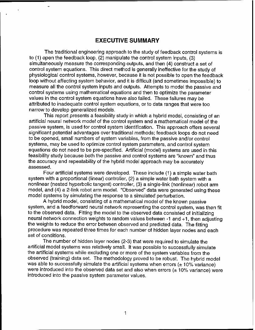
The traditional engineering approach to the study of feedback control systems is to (1) open the feedback loop, (2) manipulate the control system inputs, (3) simultaneously measure the corresponding outputs, and then (4) construct a set of control system equations. This direct method is generally ineffective for the study of physiological control systems, however, because it is not possible to open the feedback loop without affecting system behavior, and it is difficult (and sometimes impossible) to measure all the control system inputs and outputs. Attempts to model the passive and control systems using mathematical equations and then to optimize the parameter values in the control system equations have also failed. These failures may be attributed to inadequate control system equations, or to data ranges that were too narrow to develop generalized models.

This report presents a feasibility study in which a hybrid model, consisting of an artificial neural network model of the control system and a mathematical model of the passive system, is used for control system identification. This approach offers several significant potential advantages over traditional methods; feedback loops do not need to be opened, small numbers of system variables, from the passive and/or control systems, may be used to optimize control system parameters, and control system equations do not need to be pre-specified. Artificial (model) systems are used in this feasibility study because both the passive and control systems are "known" and thus the accuracy and repeatability of the hybrid model approach may be accurately assessed.

Four artificial systems were developed. These include (1) a simple water bath system with a proportional (linear) controller, (2) a simple water bath system with a nonlinear (nested hyperbolic tangent) controller, (3) a single-link (nonlinear) robot arm model, and (4) a 2-link robot arm model. "Observed" data were generated using these model systems by simulating the response to a simulated perturbation.

A hybrid model, consisting of a mathematical model of the known passive system, and a feedforward neural network representing the control system, was then fit to the observed data. Fitting the model to the observed data consisted of initializing neural network connection weights to random values between -1 and +1, then adjusting the weights to reduce the error between observed and predicted data. The fitting procedure was repeated three times for each number of hidden layer nodes and each set of conditions.

The number of hidden layer nodes (2-3) that were required to simulate the artificial model systems was relatively small. It was possible to successfully simulate the artificial systems while excluding one or more of the system variables from the observed (training) data set. The methodology proved to be robust. The hybrid model was able to successfully simulate the artificial systems when errors (± 10% variance) were introduced into the observed data set and also when errors (± 10% variance) were introduced into the passive system parameter values.

INTRODUCTION

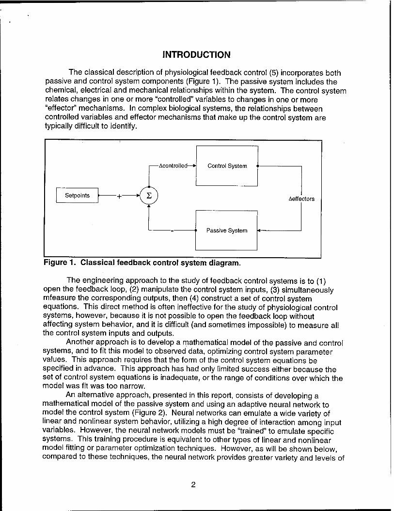
The classical description of physiological feedback control (5) incorporates both passive and control system components (Figure 1). The passive system includes the chemical, electrical and mechanical relationships within the system. The control system relates changes in one or more "controlled" variables to changes in one or more "effector" mechanisms. In complex biological systems, the relationships between controlled variables and effector mechanisms that make up the control system are typically difficult to identify.

Setpoints

-Acontrolled—►

-K Z

Control System <

Aeffectors

Passive System

Figure 1. Classical feedback control system diagram.

The engineering approach to the study of feedback control systems is to (1) open the feedback loop, (2) manipulate the control system inputs, (3) simultaneously mfeasure the corresponding outputs, then (4) construct a set of control system equations. This direct method is often ineffective for the study of physiological control systems, however, because it is not possible to open the feedback loop without affecting system behavior, and it is difficult (and sometimes impossible) to measure all the control system inputs and outputs.

Another approach is to develop a mathematical model of the passive and control systems, and to fit this model to observed data, optimizing control system parameter values. This approach requires that the form of the control system equations be specified in advance. This approach has had only limited success either because the set of control system equations is inadequate, or the range of conditions over which the model was fit was too narrow.

An alternative approach, presented in this report, consists of developing a mathematical model of the passive system and using an adaptive neural network to model the control system (Figure 2). Neural networks can emulate a wide variety of linear and nonlinear system behavior, utilizing a high degree of interaction among input variables. However, the neural network models must be "trained" to emulate specific systems. This training procedure is equivalent to other types of linear and nonlinear model fitting or parameter optimization techniques. However, as will be shown below, compared to these techniques, the neural network provides greater variety and levels of

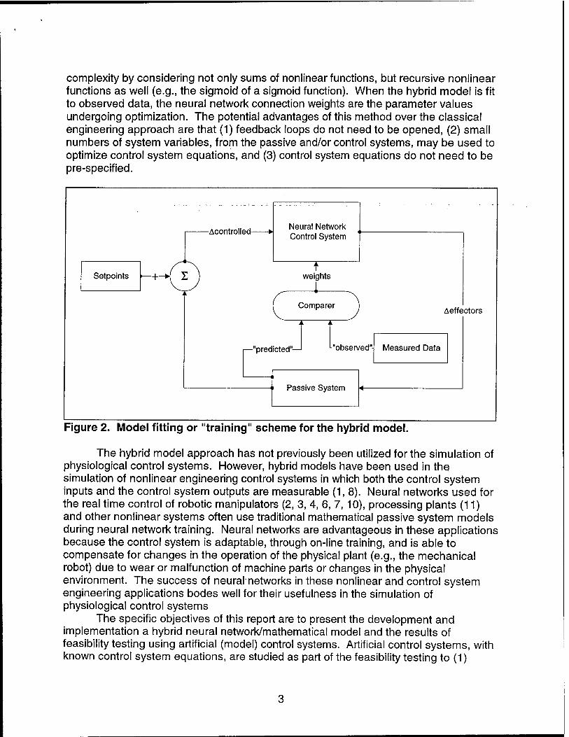
complexity by considering not only sums of nonlinear functions, but recursive nonlinear functions as well (e.g., the sigmoid of a sigmoid function). When the hybrid model is fit to observed data, the neural network connection weights are the parameter values undergoing optimization. The potential advantages of this method over the classical engineering approach are that (1) feedback loops do not need to be opened, (2) small numbers of system variables, from the passive and/or control systems, may be used to optimize control system equations, and (3) control system equations do not need to be pre-specified.

~0 A

Neural Network Control System

Aeffe ctors

Setpoints t

weights 1

Comparer

i , i L

r—"predicted- -"observed" Measured Data

Passive System

Figure 2. Model fitting or "training" scheme for the hybrid model.

The hybrid model approach has not previously been utilized for the simulation of physiological control systems. However, hybrid models have been used in the simulation of nonlinear engineering control systems in which both the control system inputs and the control system outputs are measurable (1, 8). Neural networks used for the real time control of robotic manipulators (2, 3, 4, 6, 7, 10), processing plants (11) and other nonlinear systems often use traditional mathematical passive system models during neural network training. Neural networks are advantageous in these applications because the control system is adaptable, through on-line training, and is able to compensate for changes in the operation of the physical plant (e.g., the mechanical robot) due to wear or malfunction of machine parts or changes in the physical environment. The success of neural networks in these nonlinear and control system engineering applications bodes well for their usefulness in the simulation of physiological control systems

The specific objectives of this report are to present the development and implementation a hybrid neural network/mathematical model and the results of feasibility testing using artificial (model) control systems. Artificial control systems, with known control system equations, are studied as part of the feasibility testing to (1)

determine the accuracy and repeatability of the hybrid model approach, (2) estimate the neural network architecture required to solve different control system identification problems, and (3) determine the effects of errors in the observed data and in passive system parameter values.

MATERIALS AND METHODS

ARTIFICIAL MODEL SYSTEM DEVELOPMENT Four different artificial systems (represented by mathematical models) of

increasing levels of complexity were developed and implemented in the C/C++ programming language. The first two represent water bath systems. The first of these uses a proportional (linear) controller, and the second uses a nested hyperbolic tangent function. The two other model systems represent nonlinear 1- and 2-link robot arms. Simple schematics, passive- and control-system equations for these systems are presented in Figures 3-6. Observed data were generated using these model systems by recording the response to a simulated perturbation.

For the water bath systems, (Figures 3-4), the passive system describes the response in the temperature of the system to changes in heat generation (H) and ambient temperature (Ta). The control system is responsible for adjusting H so that T is maintained at a certain "set-point" temperature, Tset. The input to the control system is the temperature T; the output is the rate of heat generation, H. Control and passive system parameter values were selected arbitrarily. The baseline rate of heat generation, Ho, was computed so that T remained at Tset unless perturbed. In two simulated experiments, the value of Ta was abruptly changed from a "neutral" value of 21 to values of 0 and 42, respectively. The responses of the system variables T and H were recorded over time.

h(T-Ta)

variables:

T=System Temperature

Ta=Environmenta! Temperature

h = Heat Transfer Coefficient (0.3)

k = Control System Gain (0.17)

H = Heat Generation (H0=4.2)

Tset=Required Temperature (35.0)

Ho = Heat Generation at (T=Tset)

t = Time

Control System

H = H,, - k(T-Tset) 'effector* variable (H)

Passive System

dT/dt = H-h(T-Ta)

'observed' data (T,H)

'controlled' variable (T)

Figure 3. Single-input, single-output water bath system with linear (proportional) controller.

h(T-Ta)

variables:

T=System Temperature

Ta=Environmental Temperature

h = Heat Transfer Coefficient (0.3)

H = Heat Generation (H (f=4.2)

Tset=Required Temperature (35.0)

Ho = Heat Generation at (T= Tset)

t = Time

Control System

H0*tanh(0.25*tanh (0.05*(T-Tset)))

'effector variable

Passive System dT/dt = H^h(T-Ta)

'observe data

'controlled' variable

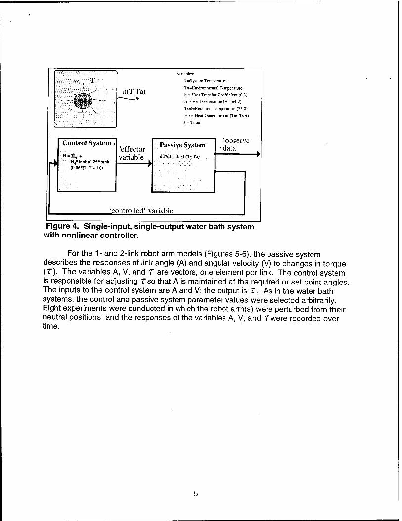
Figure 4. Single-input, single-output water bath system with nonlinear controller.

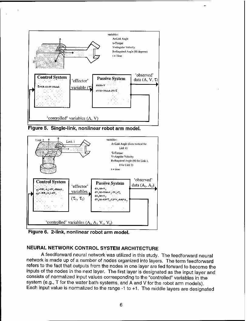
For the 1- and 2-link robot arm models (Figures 5-6), the passive system describes the responses of link angle (A) and angular velocity (V) to changes in torque (T). The variables A, V, and 1 are vectors, one element per link. The control system is responsible for adjusting Tso that A is maintained at the required or set point angles. The inputs to the control system are A and V; the output is T. As in the water bath systems, the control and passive system parameter values were selected arbitrarily. Eight experiments were conducted in which the robot arm(s) were perturbed from their neutral positions, and the responses of the variables A, V, and Twere recorded over time.

4fe variables:

A=Link Angle

T=Torque

V=Angular Velocity

R=Required Angle (90 degrees)

t = Time

Control System

T=9(R-A)-4V-10sinA

'effector'

variable CO

Passive System dA/dt=V

dV/dt=10sinA-2V+T

'observed' data (A, V, X) ►

'controlled' variables (A, V)

Figure 5. Single-link, nonlinear robot arm model.

Link 2 variables:

A=Link Angle (from vertical for

Linkl)

X=Torque

V=AnguIar Velocity

R=Required Angle (90 for Link 1,

0 for Link 2)

t = time

Control System

.^(Rj-AjMV^lÖsiriA,

tl=-.S(R1-A1)-.SV2

'effector' variables

(X„ T2)

Passive System dA^dt^,

dV/dt^OsinA.^V.+T, dAj/dl=V2

dV^dt=0.9*T,rl^*V,-.O.OS«Aj

'observed' data (A,, A2)

'controlled' variables (A, A, V,, V,)

Figure 6. 2-link, nonlinear robot arm model.

NEURAL NETWORK CONTROL SYSTEM ARCHITECTURE A feedforward neural network was utilized in this study. The feedforward neural

network is made up of a number of nodes organized into layers. The term feedforward refers to the fact that outputs from the nodes in one layer are fed forward to become the inputs of the nodes in the next layer. The first layer is designated as the input layer and consists of normalized input values corresponding to the "controlled" variables in the system (e.g., T for the water bath systems, and A and V for the robot arm models). Each input value is normalized to the range -1 to +1. The middle layers are designated

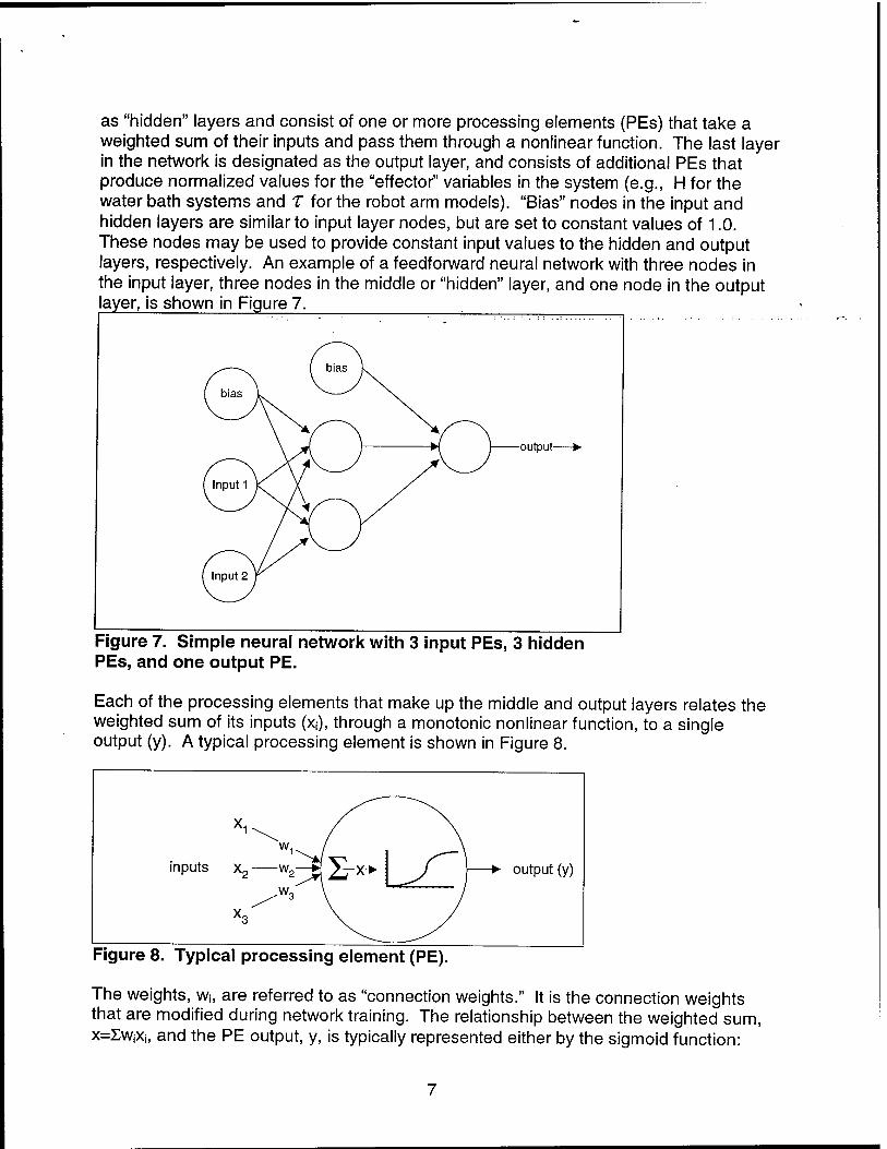
as "hidden" layers and consist of one or more processing elements (PEs) that take a weighted sum of their inputs and pass them through a nonlinear function. The last layer in the network is designated as the output layer, and consists of additional PEs that produce normalized values for the "effector" variables in the system (e.g., H for the water bath systems and T for the robot arm models). "Bias" nodes in the input and hidden layers are similar to input layer nodes, but are set to constant values of 1.0. These nodes may be used to provide constant input values to the hidden and output layers, respectively. An example of a feedforward neural network with three nodes in the input layer, three nodes in the middle or "hidden" layer, and one node in the output layer, is shown in Figure 7.

Figure 7. Simple neural network with 3 input PEs, 3 hidden PEs, and one output PE.

Each of the processing elements that make up the middle and output layers relates the weighted sum of its inputs (Xj), through a monotonic nonlinear function, to a single output (y). A typical processing element is shown in Figure 8.

-> output (y)

Figure 8. Typical processing element (PE).

The weights, Wj, are referred to as "connection weights." It is the connection weights that are modified during network training. The relationship between the weighted sum, x=ZWiXi, and the PE output, y, is typically represented either by the sigmoid function:

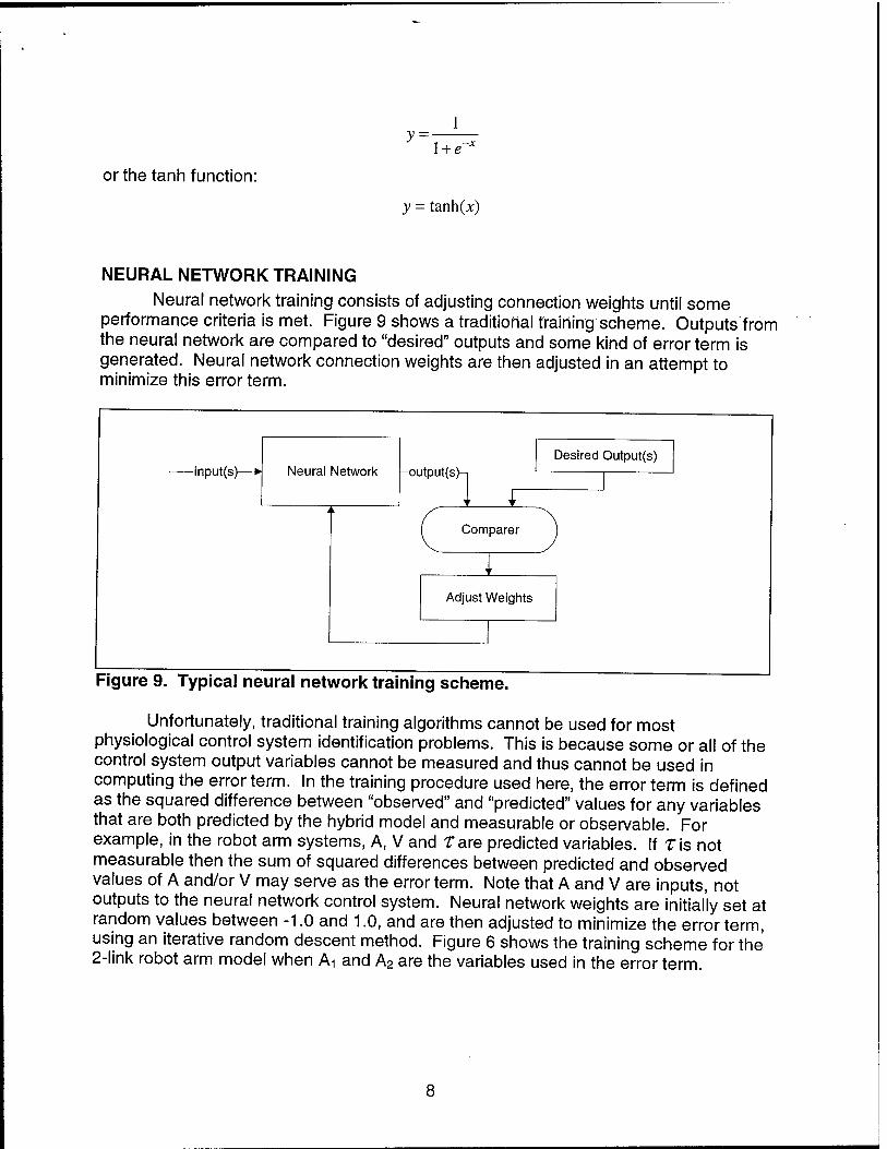
y=-

or the tanh function:

l + e'

y = tanh(jc)

NEURAL NETWORK TRAINING Neural network training consists of adjusting connection weights until some

performance criteria is met. Figure 9 shows a traditional training scheme. Outputs from the neural network are compared to "desired" outputs and some kind of error term is generated. Neural network connection weights are then adjusted in an attempt to minimize this error term.

-input(s) output(s)- Desired Output(s)

' If

Comparer

Adjust Weights

Figure 9. Typical neural network training scheme.

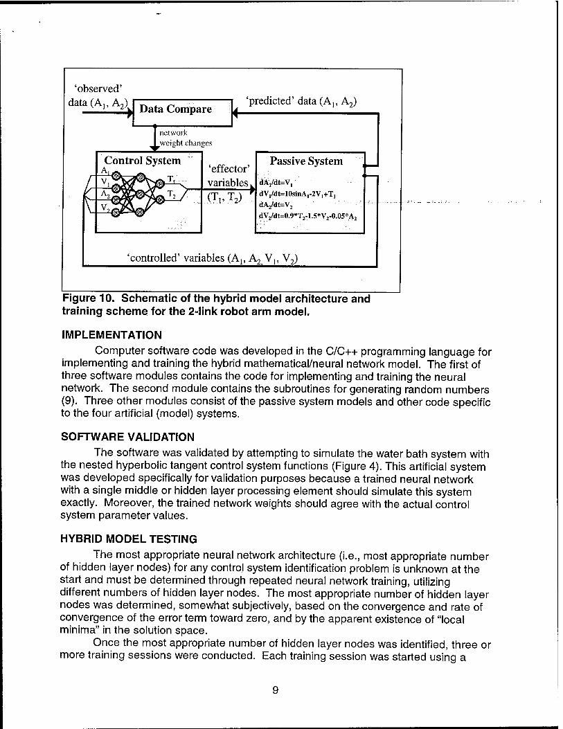
Unfortunately, traditional training algorithms cannot be used for most physiological control system identification problems. This is because some or all of the control system output variables cannot be measured and thus cannot be used in computing the error term. In the training procedure used here, the error term is defined as the squared difference between "observed" and "predicted" values for any variables that are both predicted by the hybrid model and measurable or observable. For example, in the robot arm systems, A, V and Tare predicted variables. If Tis not measurable then the sum of squared differences between predicted and observed values of A and/or V may serve as the error term. Note that A and V are inputs, not outputs to the neural network control system. Neural network weights are initially set at random values between -1.0 and 1.0, and are then adjusted to minimize the error term, using an iterative random descent method. Figure 6 shows the training scheme for the 2-link robot arm model when Ai and A2 are the variables used in the error term.

'observed' data (A,, A2) Data Compare

'predicted' data (A,, A2)

network weight changes

Control System 'effector' variables (Tl5T2),

Passive System

dkydt^, dV,/dt=10sinAr2V1+T,

dV2/dt=0.9*T2-1.5*V2-0.05*A2

'controlled' variables (At, A2 Vy, V2)

Figure 10. Schematic of the hybrid model architecture and training scheme for the 2-link robot arm model.

IMPLEMENTATION Computer software code was developed in the C/C++ programming language for

implementing and training the hybrid mathematical/neural network model. The first of three software modules contains the code for implementing and training the neural network. The second module contains the subroutines for generating random numbers (9). Three other modules consist of the passive system models and other code specific to the four artificial (model) systems.

SOFTWARE VALIDATION The software was validated by attempting to simulate the water bath system with

the nested hyperbolic tangent control system functions (Figure 4). This artificial system was developed specifically for validation purposes because a trained neural network with a single middle or hidden layer processing element should simulate this system exactly. Moreover, the trained network weights should agree with the actual control system parameter values.

HYBRID MODEL TESTING

The most appropriate neural network architecture (i.e., most appropriate number of hidden layer nodes) for any control system identification problem is unknown at the start and must be determined through repeated neural network training, utilizing different numbers of hidden layer nodes. The most appropriate number of hidden layer nodes was determined, somewhat subjectively, based on the convergence and rate of convergence of the error term toward zero, and by the apparent existence of "local minima" in the solution space.

Once the most appropriate number of hidden layer nodes was identified, three or more training sessions were conducted. Each training session was started using a

different (random) set of initial network weights. Observed control system input-output relationships were then compared with input-output relationships from the neural network. Comparisons were made to determine the accuracy of the predicted input- output relationships, and also the repeatability of the hybrid model system training method (i.e., the ability for each training session to reach the same solution). These comparisons were then repeated under two conditions to determine the robustness of the method: 1) a random 10% error in "observed" data (error values randomly selected from a Gaussian distribution with +/-10% variance); and 2) a random 10% error in passive system model parameter values (error values randomly selected from a Gaussian distribution with +/-10% variance).

Finally, tests were conducted to determine the ability of the hybrid model'to' identify the control system using incomplete data sets. Although it is possible using artificial systems to "know" or "measure" the responses of all control system input and output variables, this is certainly not the case for most physiological systems. For this test, variables were dropped from the set of observed data and the tests repeated (e.g., for the 2-link robot arm model, all variables except Ai and A2 are excluded from the set "observed" data).

RESULTS

LESSONS LEARNED For each control system identification problem, simulations were conducted

using different numbers of middle-layer nodes, and different sets of variables included in the "observed" data set. Each simulation was repeated 3 times (denoted as Tests 1, 2, and 3), starting at different random initial weights each time. It was necessary to normalize observed and predicted data so that the training would not be biased toward variables that take on larger values. It was also necessary to normalize neural network inputs and outputs so that each variable carried the same degree of "importance" in network training. In addition, the training data set had to induce a sufficiently broad range of system responses so as to get a reproducible set of control system input- output relationships. For example, for the linear water bath system, it was necessary to train under both hot (Ta above normal) and cold (Ta below normal) conditions.

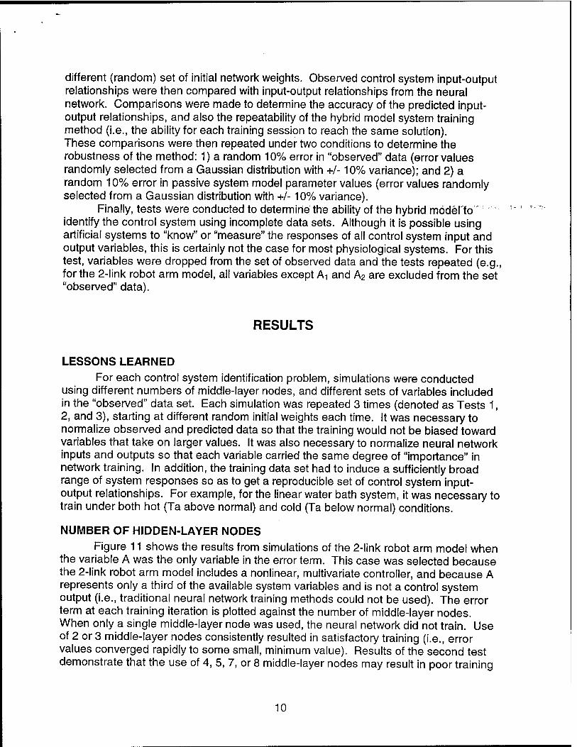
NUMBER OF HIDDEN-LAYER NODES Figure 11 shows the results from simulations of the 2-link robot arm model when

the variable A was the only variable in the error term. This case was selected because the 2-link robot arm model includes a nonlinear, multivariate controller, and because A represents only a third of the available system variables and is not a control system output (i.e., traditional neural network training methods could not be used). The error term at each training iteration is plotted against the number of middle-layer nodes. When only a single middle-layer node was used, the neural network did not train. Use of 2 or 3 middle-layer nodes consistently resulted in satisfactory training (i.e., error values converged rapidly to some small, minimum value). Results of the second test demonstrate that the use of 4, 5, 7, or 8 middle-layer nodes may result in poor training

10

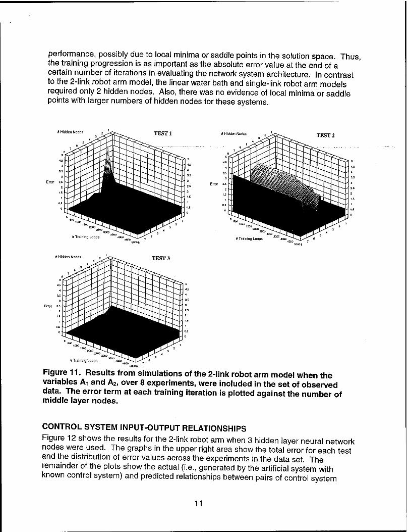
performance, possibly due to local minima or saddle points in the solution space. Thus, the training progression is as important as the absolute error value at the end of a certain number of iterations in evaluating the network system architecture. In contrast to the 2-link robot arm model, the linear water bath and single-link robot arm models required only 2 hidden nodes. Also, there was no evidence of local minima or saddle points with larger numbers of hidden nodes for these systems.

# Hidden Nodes TEST1 # Hidden Nodes TEST 2

# Training Loops

# Hidden Nodes

It Training

Figure 11. Results from simulations of the 2-link robot arm model when the variables A, and A2, over 8 experiments, were included in the set of observed data. The error term at each training iteration is plotted against the number of middle layer nodes.

CONTROL SYSTEM INPUT-OUTPUT RELATIONSHIPS Figure 12 shows the results for the 2-link robot arm when 3 hidden layer neural network nodes were used. The graphs in the upper right area show the total error for each test and the distribution of error values across the experiments in the data set. The remainder of the plots show the actual (i.e., generated by the artificial system with known control system) and predicted relationships between pairs of control system

11

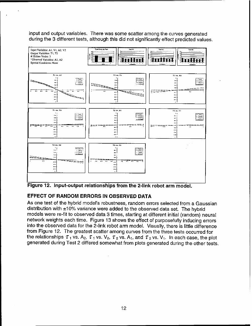
input and output variables. There was some scatter among the curves generated during the 3 different tests, although this did not significantly effect predicted values.

Input Variables: Al, VI, A2. V2 Output Variables: Tl, T2 # Hidden Nodes: 3 "Observed Variables: Al, A2 Special Conditions: None

1:

Total Error, by T**t

■ _ 1 ■ H ■ ■ ■ 15: llllllll

— Tittl — T»it2 — T«it3 ■»■ Actml

T2 v*. A1

-•-Ttitf

" ■—T»it2 •--Tiit3 -—Aetu»!

0.2

■S ;— ■°> *.l ..•

*•'* ■0.1

— T»tu —'T«tl2 — T«it3

T2 V a. V2

» —-Ttiti

— T.«I3 — Actuil

z

Figure 12. Input-output relationships from the 2-link robot arm model.

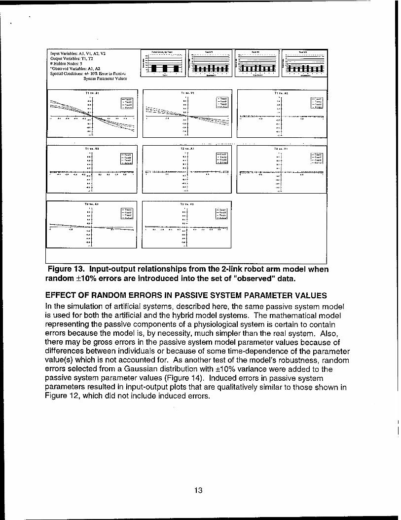
EFFECT OF RANDOM ERRORS IN OBSERVED DATA As one test of the hybrid model's robustness, random errors selected from a Gaussian distribution with ±10% variance were added to the observed data set. The hybrid models were re-fit to observed data 3 times, starting at different initial (random) neural network weights each time. Figure 13 shows the effect of purposefully inducing errors into the observed data for the 2-link robot arm model. Visually, there is little difference from Figure 12. The greatest scatter among curves from the three tests occurred for the relationships T^ vs. A2, Ti vs. V2, T2 vs. A1( and T2 vs. VL In each case, the plot generated during Test 2 differed somewhat from plots generated during the other tests.

12

Input Variables: Al, VI, A2, V2 Output Variables: Tl, T2 # Hidden Nodes: 3 "Observed Variables: Al, A2 Special Conditions: +/- 10% Error in Passive

System Parameter Values

Totil Error, byT»t

■ ■ ■ H H H

T1 v .V1

SäSss^^J

— Tiill — T«m12

— T.H3

:: ~'~"~~--^ir--t:---

T2 V ». A1

:: — TtiU — Aeluil

z

T2 V«. V2

— To 0.1 — To •12

IM

— To

Ml

«

■8.4

0.1 0.* 0.0

....

Figure 13. Input-output relationships from the 2-link robot arm model when random ±10% errors are introduced into the set of "observed" data.

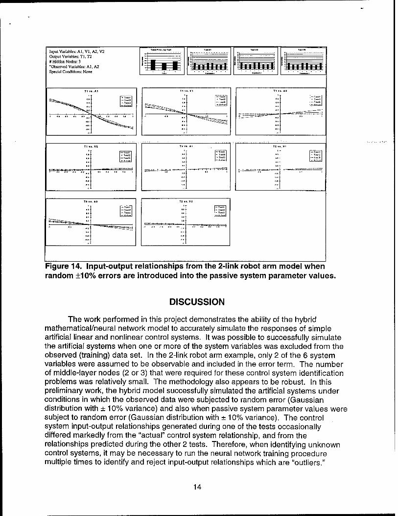
EFFECT OF RANDOM ERRORS IN PASSIVE SYSTEM PARAMETER VALUES In the simulation of artificial systems, described here, the same passive system model is used for both the artificial and the hybrid model systems. The mathematical model representing the passive components of a physiological system is certain to contain errors because the model is, by necessity, much simpler than the real system. Also, there may be gross errors in the passive system model parameter values because of differences between individuals or because of some time-dependence of the parameter value(s) which is not accounted for. As another test of the model's robustness, random errors selected from a Gaussian distribution with ±10% variance were added to the passive system parameter values (Figure 14). Induced errors in passive system parameters resulted in input-output plots that are qualitatively similar to those shown in Figure 12, which did not include induced errors.

13

Input Variables: Al, VI, A2, V2 Output Variables: Tl, T2 # Hidden Nodes: 3 "Observed Variables: Al, A2 Special Conditions: None

III 11 H=t

Ss

T1 v.. VI

ii - T««K

— T»i13 — Aclual

~~"

:: "** 333

fli ---T»i« — T««0

..< 0.2 _-

-■■- "" ""'"

■0.«

-T.H2 -T..I3

T2 v 1. A1

— T.*I2 -r.-T.ll3

!:

T2 v ■ . V2

•j — Ttntl — T.itZ — T.«IS

:i: » »7T--A "• .V —t

Figure 14. Input-output relationships from the 2-link robot arm model when random ±10% errors are introduced into the passive system parameter values.

DISCUSSION

The work performed in this project demonstrates the ability of the hybrid mathematical/neural network model to accurately simulate the responses of simple artificial linear and nonlinear control systems. It was possible to successfully simulate the artificial systems when one or more of the system variables was excluded from the observed (training) data set. In the 2-link robot arm example, only 2 of the 6 system variables were assumed to be observable and included in the error term. The number of middle-layer nodes (2 or 3) that were required for these control system identification problems was relatively small. The methodology also appears to be robust. In this preliminary work, the hybrid model successfully simulated the artificial systems under conditions in which the observed data were subjected to random error (Gaussian distribution with ± 10% variance) and also when passive system parameter values were subject to random error (Gaussian distribution with ± 10% variance). The control system input-output relationships generated during one of the tests occasionally differed markedly from the "actual" control system relationship, and from the relationships predicted during the other 2 tests. Therefore, when identifying unknown control systems, it may be necessary to run the neural network training procedure multiple times to identify and reject input-output relationships which are "outliers."

14

The results from this study using artificial systems is encouraging in terms of the potential use of this methodology for the study of physiological systems. Physiological systems are adaptive, the control systems are quantitatively unknown, and control system outputs are frequently inaccessible for measurement, precluding the use of more traditional methods. Also, errors can be expected both in measured data as well as in parameter value estimates in even the most complete mathematical models. A reasonable next step would be to use a neural network to model a physiological control system in which the inputs and outputs are accessible for measurement. The results of this parameter optimization could be compared directly with results from statistical model fitting procedures. The next step would be to utilize a hybrid neural network/ mathematical model of the entire system and to repeat the model fitting procedure using variables other than the control system outputs in the error term.

15

REFERENCES

1. Beale, M. and H. DeMuth. Preparing controllers for nonlinear systems. AJ Expert, 7(7): 42-47, 1992.

2. Bürgin, G. Using cerebellar arithmetic computers. Al Expert. 7(6): 32-42, 1992.

3. Guez, A., J. Eilbert and M. Kam. Neural network architecture for control. IEEE Control Systems Magazine. 8: 22-24, 1988.

4. Guez, A., J. Eilbert and M. Kam. Neuromorphic architectures for fast adaptive robot control. IEEE Conference on Robotics and Automation, Volume 1, Institute of Electronic and Electrical Engineers, 1988, pp. 140-143.

5. Hardy, J.D. and J.A.J. Stolwijk. Regulation and control in physiology. Medical Physiology. 12th Edition, Volume 1, Chapter 34, V.B. Mountcastle (Ed.). 1968, pp. 591- 610.

6. Kawato, M., Y. Uno, M. Isobe and R. Suzuki. Hierarchical neural network model for voluntary movement with application to robotics. IEEE Control Systems Magazine. 8:8-15,1988.

7. Kuperstein, M. Generalized neural model for adaptive sensory-motor control of single postures. Automation, 1: 140-143, 1988.

8. McCullough, C.L. An anticipatory fuzzy logic controller utilizing neural net prediction. Simulation. 58(5): 327-332, 1992.

9. Press, W.H., B.P. Flannery, S.A. Teukolsky and W.T. Vetterling. Numerical Recipes. New York: Cambridge University Press, 1986.

10. Psaltis, D., A. Sideris and A.A. Yamamura. A multilayer neural network controller. IEEE Control Systems Magazine. 8: 17-21, 1988.

11. Sabharwal, A., N.V. Bhat, and T. Wada. Integrate empirical and physical modeling. Hydrocarbon Processing (International edition), 76: 105-108, 1997.

16