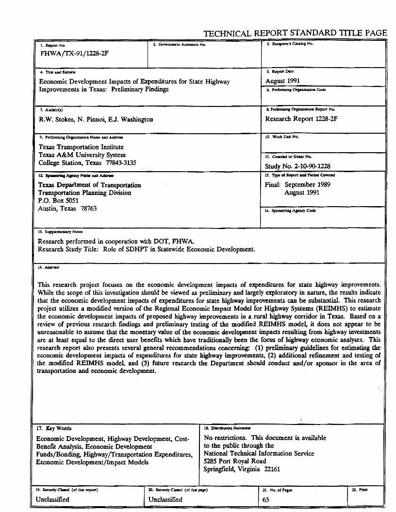
TECHNICAL REPORT STANDARD 1TILE PAGE 1. Report No. l. ~ Aa:eaion No. 3. R.ecipftl'i Catalog No.

FHW AffX-91/1228-2F

Economic Development Impacts of Expenditures for State Highway Improvements in Texas: Preliminary Fmdings

S. Report Date

August 1991

7. AUUlor(•)

R.W. Stokes, N. Pinno~ EJ. Washington

9. Performin& Orpnizatlon N...,.. ud Addrm

Texas Transportation Institute Texas A&M University System College Station, Texas 77843-3135

12. si-wm& Afl'lll=1 Name ud Addrm

Texas Depaitment of Transportation Transportation Planning Division P.O. Box 5051 Austin, Texas 78763

IS. Supplcmeawy NOia

Research performed in cooperation with DOT, FHW A.

&. hrformi.Da Orpnizatioa Report No.

Research Report 1228-2F

10. Wori< Uai! No.

11. Colllnd or Gram No.

Study No. 2-10..90-1228 13. 1)pe of Report and Period ea-m

Final: September 1989 August 1991

Research Study Title: Role of SDHPT in Statewide Economic Development.

This research project focuses on the economic development impacts of expenditures for state highway improvements. While the scope of this investigation should be viewed as preliminary and largely exploratory in nature, the results indicate that the economic development impacts of expenditures for state highway improvements can be substantial. This research project utilizes a modified version of the Regional Economic Impact Model for Highway Systems (REIMHS) to estimate the economic development impacts of proposed highway improvements in a rural highway corridor in Texas. Based· on a review of previous research fmdings and preliminary testing of the modified REIMHS model, it does not appear to be unreasonable to assume that the monetary value of the economic development impacts resulting from highway ·investments are at least equal to the direct user benefits which have traditionally been the focus of highway economic analyses. This research report also presents several general recommendations concerning: (1) preliminary guidelines for estimating the economic development impacts of expenditures for state highway improvements, (2) additional refinement and testing of the modified REIMHS model, and (3) future research the Department should conduct ud/or sponsor in the area of transportation and economic development.

17. Key Words

Economic Development, Highway Development, Cost· Benefit Analysis, Economic Development Funds/Bonding, Highway /Transportation Expenditures, Economic Development/Impact Models

No restrictions. This document is available to the public through the National Technical Information Service 5285 Port Royal Road Springfield, Virginia 22161

19. Securily Clalait. (of ll:lir report)

Unclassified

20. Securily C'lmll. (of Ibis Jiii")

Unclassified

21. No. of Pages

65

ECONOMIC DEVELOPMENT IMPACTS OF EXPENDITURES FOR STATE HIGHWAY IMPROVEMENTS IN TEXAS

Preliminary Findings

by

Robert W. Stokes Associate Research Planner

Nat Pinnoi Research Associate

and

Earl J. Washington Assistant Research Planner

Research Report No. 1228·2F Research Study No. 2· 10-90-1228

Role of TxDOT in Statewide Economic Development

Sponsored by

Texas Department of Transportation

in cooperation with the U.S. Department of Transportation

Federal Highway Administration

Texas Transportation Institute The Texas A&M University System

College Station, TX 77843·3135

August 1991

METRIC (SI*) CONVERSION FACTORS APPROXIMATE CONVERSIONS TO SI UNITS APPROXIMATE CONVERSIONS TO SI UNITS

Symbol When You Know Multiply lly To Find Symbol Symbol When You Know Multiply BJ To Find Symbol

LENGTH LENGTH .. ... " -

mllllmetres 0.039 Inches In In Inches 2.54 centimetres

.. mm cm = ..

ft

" feet 0.3048 = m metres 3.28 feet metres m ..

1.09 yards yd - =-- " m metres yd yards 0.914 metres m = • km kilometres 0.621 miles ml ml mllea 1.61 kilometres km - I - ~

= !I AREA - = -AREA .. = :!

- mm1 millimetres squared 0.0016 square Inches ln1

ln1 square Inches 845.2 centimetres squared cm• -- !:: m' metres squared 10.784 square feet ft1

ft' square feet 0.0929 -metres squared m' - km1 kilometres squared 0.39 square mlles ml1

yd• square yards 0.836 metres squared m• - ha hectares (10 000 m') 2.53 acres ac

ml' square miles 2.59 kilometres squared km' -ac acres 0.395 hectares ha - MASS (weight)

-... - g grams 0.0353 ounces oz

MASS (weight) - kg kilograms 2.205 pounds lb --- Mg megagrams (1 000 kg) 1.103 short tons T oz ounces 28.35 grams g --lb pounds 0.454 kilograms kg .. -T short tons (2000 lb) 0.907 megagrams Mg VOLUME

- ml millllltres 0.034 fluid ounces fl oz - l lltres 0.284 gallons gal VOLUME

... - .. mi metres cubed 35.315 cubic feet ft' -- m• metres cubed 1.308 cubic yards yd* fl oz fluid ounces 29.57 mlllllltres ml - .. gal gallons 3.785 Hires l -ft' cubic feet 0.0328 metres cubed m'

.. ... TEMPERATURE (exact) =--- = yd' coble yards 0.0765 metres cubed m• -

NOTE: Volumes greater than 1000 L shall be shown In m'. - "C Celsius 915 (then Fahrenheit Of

- ... temperature add 32) temperature

Of - .. "F 32 98.8 212 -- ~I I I ? I I ~ ~ I I I l!" I t. I

1~ I I I

1~ I I .~J TEMPERATURE (exact) 3 -i - = fi

I I I 1 I I 1 t i I 100 -40 -20 0 20 40 80 80 = .. - "C 37 "C Of Fahrenheit 5/9 (after Celslus "C

temperature subtracting 32) temperature These factors conform to the requirement of FHWA Order 5190.1A.

• SI Is the symbol tor the lntematlonal System of Measurements

IV

ABSTRACT

This research project focuses on the economic development impacts of expenditures for state highway improvements. While the scope of this investigation should be viewed as preliminary and largely exploratory in nature, the results indicate that the economic development impacts of expenditures for state highway improvements can be substantial. This research project utilizes a modified version of the Regional Economic Impact Model for Highway Systems (REIMHS) to estimate the economic development impacts of proposed highway improvements in a rural highway corridor in Texas. Based on a review of previous research findings and preliminary testing of the modified REIMHS model, it does not appear to be unreasonable to assume that the monetary value of the economic development impacts resulting from highway investments are at least equal to the direct user benefits which have traditionally been the focus of highway economic analyses. This research report also presents several general recommendations concerning: (1) preliminary guidelines for estimating the economic development impacts of expenditures for state highway improvements, (2) additional refinement and testing of the modified REIMHS model, and (3) future research the Department should conduct and/or sponsor in the area of transportation and economic development.

Key Words: Economic Development, Highway Development, Cost-Benefit Analysis, Economic Development Funds/Bonding, Highway Transportation Expenditures, Economic Development/Impact Models

v

vi

IMPLEMENTATION STATEMENT

This research project focuses on the economic development impacts of expenditures for state highway improvements. While the scope of this investigation should be viewed as preliminary and largely exploratory in nature, the results indicate that the economic development impacts of expenditures for state highway improvements can be substantial. The results of this study should be useful to the Department in developing a more comprehensive approach to evaluating various state highway improvement programs and projects.

DISCLAIMER

The contents of this report reflect the views of the authors who are responsible for the opinions, findings, and conclusions presented herein. The contents do not necessarily reflect the official views or policies of the Federal Highway Administration or the Texas Department of Transportation. This report does not constitute a standard, specification, or regulation. This report is not intended for construction, bidding or permit purposes.

vii

viii

TABLE OF CONTENTS

Abstract ...................................................................................................................................... . v

Implementation Statement .................................................................................................... . .

VI

Disclaimer ................................................................................................................................ . VI

I. In.troduction ................................................................................................................. . 1

Background ..... .......................... ................................. ................. ................. .... 1 Study Objectives .............................................................................................. 3

II. State-of-the-Art ........................................................................................................... . 5

Literature Review ........................................................................................... 5 Transportation and Economic Development Programs in Other States ................................................................................................. 8 Transportation and Economic Development Impact Models ................ 11

III. The Regional Economic Impact Model for Highway Systems (REIMHS) ...... 17

Ov'erview ....................................................................••..•.................................. 17 Data Requirements ........................................................................................ 20 Data Sources .................................................................................................... 21 Model Structure .............................................................................................. 22 Previous Applications in Texas .................................................................... 31 Limitations of REIMHS ................................................................................ 32 The Modified REIMHS Model ................................................................... 35

IV. Preliminary Analysis of Economic Impacts of Highway Expenditures in Texas ............................................................................................... . 43

Ov'erview ............................................................................................................ 43 Study Corridor ................................................................................................. 43 Summary of Test Application of the Modified REIMHS Model ......... 45

v. Conclusions and Recommendations ....................................................................... . 49

Conclusions ...................................................................................................... 49 Recommendations ........................................................................................... 50

References . ... ... . ....... .. ... .......... ................ ............. .............. ...... .... ........ ............... ........................ 5 5

ix

x

I. INTRODUCTION

Background

In recent years, the Texas Department of Transportation (TxDOT) has begun to expand its

mission to include the use of highway improvements to encourage economic growth and

development in the state. Highway improvements, either in the form of a new highway or

the upgrading of an existing one, can generate changes in the functioning of an economy.

Economic effects can be beneficial, where accessibility is improved, travel time and costs are

reduced, or land values rise; or they can be adverse, where land values decrease or

congestion on feeder roads increases. It is important to identify, to the extent possible,

where highway improvements are likely to be most beneficial, who or what groups realize

the gains, and who or what groups bear the costs (including the costs of foregoing one

project in favor of another).

The Department frequently receives requests to conduct intercity route studies. The

requests for these studies frequently come from local governments and/ or the private sector

and are typically promoted on the basis that the new routes would result in improved

movement of people and goods and produce economic benefits. The proposed new roadway

in the Austin-San Antonio corridor, for example, has been advocated as a means to

accommodate recent and projected traffic growth in the I-35 corridor between Austin and

San Antonio. The proposed roadway would also improve the accessibility cf thousands of

acres of undeveloped land and foster additional development and economic growth in the

corridor. Similarly, the proposed new roadway in the Austin-College Station corridor is

being promoted on the basis of its ability to improve the quality of the highway system

serving the two cities and to stimulate additional cooperative efforts between Texas A&M

University and the University of Texas.

At the present time, TxDOT is developing a State Highway Trunk System but does

not currently have procedures to systematically assess the traffic and economic development

1

impacts of proposed intercity highways. As a result, requests for intercity route studies are

addressed on a case-by-case basis. At the present time, it is difficult to anticipate the timing

and scope of these requests and incorporate them into the state's transportation planning

and programming process. This approach to responding to these requests requires a great

deal of TxDOT staff time and resources. There is a need to develop procedures and/ or

policies to evaluate these requests for highway route studies within the Department's

statewide transportation planning process.

Tue state-of-the-art in modeling the relationships between transportation and its

physical, socia~ and economic environments is largely "one-dimensional." For example, the

number of trips produced and attracted by an area can be estimated from information

describing the socioeconomic characteristics of the area. However, the problem of

estimating the nature and magnitude of the socioeconomic impacts that result from

improvements in the transportation system is much more complex and is not understood

nearly as well as the relationships between economic activity and travel demand. As a

result, the various interest groups that may be involved in highway improvement projects

that are intended to promote economic growth and development often have very different

perceptions of the potential magnitude of the economic impacts of highway improvements.

Transportation planners and engineers can employ a number of "standard" procedures

(e.g., benefit-cost analysis) to assess the relative cost-effectiveness of alternative

transportation improvements. However, benefit-cost analysis, and most of the other

traditional economic analysis procedures, typically does not address the complete spectrum

of social and economic impacts of highway improvements. In addition, there are several

methodologies which can be used to examine the relationships between transportation and

economics at the regional level. However, there are no widely accepted procedures for

quantifying the economic development potentials of transportation improvements within

individual travel corridors.

This research report focuses on the relationships between the state's transportation

expenditures for intercity highways and economic development. The relationships between

2

economic development and changes in accessibility, travel time, or land values that result from

intercity highways are not explicitly addressed. However, the results of this research could

provide a useful point of departure for future research efforts directed at quantifying the

relationships between changes in accessibility, travel time or land values, and economic

development.

Study Objectives

The overall goal of this research effort is to develop procedures and/or guidelines to assess

the economic impacts of intercity highways. Specific study objectives are:

1) Review procedures used by other states to identify, prioritize, and select intercity

highway improvements that are intended to foster economic development.

2) Identify current analytical techniques for assessing the economic development

impacts of expenditures on intercity highways.

3) Develop the data bases needed to calibrate and implement these procedures for

use in selected travel corridors in Texas.

4) Develop guidelines for use in assessing the economic development impacts of

expenditures on intercity highways in Texas.

5) Develop procedure(s) for incorporating these guidelines into the state's existing

planning and decision-making process.

A previous research report (1) presented a review of the literature, a survey of

current practices in other state departments of transportation to foster economic

development through highway improvements, and the identification of analytic techniques

for assessing the economic impacts of expenditures for highway improvements. Specifically,

3

that report addressed study objectives 1 and 2. The key findings of the previous research

report are briefly summarized in the following chapter of this report.

The principle focus of this report is on those phases of the research directed at the

primary study objectives; e.g., objectives 3, 4, and 5. The scope of this investigation should

be viewed as exploratory and, therefore, preliminary in nature, as the findings are based on

the results of using a single model to estimate the economic development impacts of

highway expenditures in a very limited number of rural highway corridors. This study

provides preliminary, planning-level guidelines which could be used to estimate the

monetary magnitude of the economic development impacts of various highway investment

programs. The results do indicate that the economic development impacts of expenditures

for highway improvements can be substantial.

4

II. STATE-OF-TIIE-ART

Literature Review

The connection between highway improvements and economic development is both obvious

and elusive. Conventional wisdom holds that ample, well maintained highways, streets, and

roads are important to an area's development potential because they provide access to

resources, goods, and markets. In any form of economic activity, accessibility is a critical

need. However, the precise impact of a particular transportation improvement is often

times difficult to assess. Also, a variety of external factors complicate an understanding of

this linkage. Some of these are availability and cost of land, labor, and capital; relative tax

rates; environmental and general life quality; and the presence of needed services and other

types of infrastructure. A reasonable supposition is that good transportation is a necessary

but not sufficient condition for economic development to occur. Put another way,

transportation facilities contribute significantly to a competitive advantage of an area. The

stronger the overall competitive advantage an areas has, the more likely employment -

generating investment is to occur (2).

The role of highway development in economic growth has been the subject of

considerable analysis. Briggs (J.) demonstrated, using regression analysis, that the location

of interstate highways has a positive effect on economic growth through population

migration and employment change. Siccardi (~) documents the legislative history of federal

attempts to stimulate growth through transportation improvements. Siccardi concludes that

economic growth is promoted by increasing accessibility to meet specific objectives, such as

improving access to airports, hospitals, and other community service functions. Additionally,

he points out that population receives beneficial growth effects from highway improvements,

and this will, in fact, become a positive stimulus to prosperity.

Lichter and Fuguitt (~) concur in their examination of demographic response to the

interstate highways in non metropolitan areas stating:

5

The presence of good transportation appears to be a necessary part of any adequate explanation of nonmetropolitan population growth generated by inmigration. This effect is posited to operate through employment change in manufacturing, non local trade and services, and tourist related activity.

The effect of highway development on improved accessibility also has a positive

impact on property values. Miller (n) discussed the concept of accessibility and the resulting

appreciation of property. He asserts that the relative location of a piece of property is a key

factor in enhancing property values. Using time series and regression techniques, Langley

(1) and Palmquist (.8) demonstrate how proximity to major thoroughfares increases adjoining

property values. Specifically, Palmquist predicts a 15 to 17 percent increase in property

values resulting from being directly accessible to a highway segment. Grossman and Levin

(2) examined the effects of highways on distressed or redevelopment areas and suggest that

good highway transportation is at least as important in distressed manufacturing centers as

in any other urban area; in addition, there are a number of instances of smaller urban

centers so located that their economies can be directly stimulated by an improvement of

their connections to a nearby, larger metropolitan area with a stronger, more diversified

economy. Improved highway transportation is a potentially vital factor in combating the

effects of economic decline in a major distressed area. Grossman and Levin (2) also suggest

that high quality highways are one of the most important elements in economic development

in modern American communities. Although good highways alone are not sufficient to

insure economic improvement in competition with other areas, they are a necessity to any

area to insure its attractiveness to new industry, its ability to retain existing industry, and its

overall efficiency as a place to live and work.

A National Cooperative Highway Research Program (NCHRP) study (10) points out

that highway improvements, either in the form of a new highway or the upgrading of an

existing one, unquestionably generate changes in the functioning of an economy. To some

extent the welfare and/or income position of some individuals and/or firms will be altered.

Economic effects can be beneficial (positive), where travel time and cost are reduced or

land values rise; or they can be adverse (negative), where land values decrease or congestion

6

on feeder roads increases. Rarely is an economic impact clearly all beneficial or all harmful

within a community.

Some research results minimize the significance of the role of transportation facilities

in the promotion of economic development. For example, Mills (11) examined the effects

of beltways on the location of residences and selected work places and reported that

beltways and probably transportation facilities in general are, at most, one of many

influences on the pattern of urban development, and policies to support revitalization of

central cities might be better implemented by using beltways or other transportation

facilities to support measures such as land use controls that bear more directly on urban

development.

Eagle and Stephanedes (12) addressed the causality relationship between highway

improvements and economic development and concluded:

Increases in highway expenditures do not in general lead to increases in employment other than temporary increases in the year of construction. However, in locations that are economic centers of the state, highway expenditures do have a positive long term effect, that is, employment increases more than it would for the normal trend of the economy.

Baird and Lipsman (ll) have contested the significance of the relationship between

highway transportation and economic development stating:

Clearly, major highway system changes promote change in local and regional economies, but whether transportation infrastructure investment causes long­term economic development remains in question.

Wilson et al. ( 14) report similar findings in an examination of the role of

transportation in regional economic growth. The authors concluded:

Transportation improvements have been cited as having important effects on political unity, social cohesion, economic growth, specialization, and price stability, as well as an attitudinal change. Yet ... precisely opposite effects are equally plausible.

7

Transportation and Economic Development Programs in Other States

Many states simply incorporate economic development objectives into their normal

programming process and do not have special funds or programs for the specific purpose

of fostering economic development. The nature of involvement in economic development­

related activities by state transportation agencies is presented in Table 1. Thirty-six states

explicitly take economic development into account in their highway programming activities.

Of these states, 14 incorporate economic development objectives into their normal

programming process but do not have special funds or programs for the specific purpose of

fostering economic development. The methods used range from informal petitions on the

part of local governments for priority programming to point systems for ranking projects.

A surprisingly large number of states, 22, have categorical funding or bonding

authority for economic development. Iowa, for example, has a dedicated two-cent motor

fuel tax, the proceeds of which flow into a special fund. Programs vary in scale from

Maine's $400,000 industrial park matching program (to supplement private sector funds) to

more extensive efforts, such as those in Florida, Iowa, Massachusetts, Michigan, and

Washington (see Table 2).

Eleven states' programs are oriented primarily toward making industrial parks more

accessible. These programs supplement local and private funding sources in financing the

construction of such improvements as interchanges, frontage roads, or other access roads.

In their industrial park programs, some states specify funding limitations based on the

amount of local or private funds contributed or on the number of jobs created. South

Dakota, for example, requires:

• A commitment to actual construction of the industrial facility in the near future.

• A committed capital investment of at least five times the required state participation costs.

Total employment for all facilities in the industrial park of at least 50.

8

State

Alabama Alaska Arizona Arkansas California Colorado Connecticut Delaware Florida Georgia Hawaii Idaho lliinois Indiana Iowa Kansas Kentucky Louisiana Maine Maryland Massachusetts Michigan Minnesota Mississippi Missouri Montana Nebraska Nevada New Hampshire New Jersey New Mexico New York North Carolina North Dakota Ohio Oklahoma Oregon Pennsylvania Rhode Island South Carolina South Dakota Tennessee Texas Utah Vermont Virginia Washington West Virginia Wisconsin Wyoming

Sources: (1,1).

Notes: 1.

2.

3. 4.

5.

Table L Sanmuu:y of State DOT Involvement in Economic Dnelopmeat Programs

Economic Development Special Industrial

Objectives in Economic Development Park Road Quick-Response

Programming1 Funds/Bondin!( Program3 Capabilities4

• • • *

• • * • * • .

* • • • • • • • • • • • . • * . • • • • • . * • • • • • •

• • .s

•

• • • • • •

* • • * . *

• • • * * * *

• • • • . • . * • . • • * •

"Economic Development Objectives in Programming" means that the state specifically takes economic development into account in its capital programming process or has special highway programs to encourage economic development. "Special Economic Development Funds/Bonding" means that the state has a categorical funding source or bonding authority for economic development or industrial park roads. "Industrial Park Program" means that the state has a special program dedicated to constructing this type of road. "Quick-Response Capabilities" means that the state has the ability to expedite economic development-related road projects. Expedites environmental review for economic development projects.

9

Table 2. Details of Special State Highway Economic Development Programs

Approximate Annual Budget State ($Million) Program Name/Description

Alabama No annual budget Single-bond issue of $2.5 million Alaska No annual budget State economic development program Arkansas Not reported Industrial access roads Florida $10.0 E.conomic Development Transportation Fund lliinois $4.4 Five-year average. Part of "Build Illinois" Iowa $7.5 Six-year average. "RISE" program Kansas $3.0 E.conomic Development Fund Kentucky No fixed budget Industrial access road program Louisiana No fixed budget Discretionary funds Maine $0.4 Federal funds Massachusetts $10.00 Public Works and E.conomic Development Program Michigan $13.3 Three-year average. E.conomic Development Program Minnesota No annual budget . Municipal bonding, reimbursed by state New York $5.0 Industrial Access Program North Carolina $2.0 State E.conomic Development Program Oklahoma $1.6 Industrial Access Road Program South Dakota $0.5 Industrial Park Construction Program Virginia $3.0 Industrial Access Fund Washington $10.0 Community E.conomic Revitalization Board West Virginia No fixed budget Contingency funds Wisconsin $4.9 Proposed "AHPAD" Program Wyoming $1.0 Industrial Road Program

Sources: (!,~.

• Local participation in funding of industrial park roads of at least 20 percent of the approved state project construction budget.

• Dedication of the roadway and adjacent right-of-way to public use.

State participation limited to roads within the industrial park that are one mile or less in length.

Similarly, Virginia stipulates that unmatched state highway funding shall not exceed

10 percent of the total private capital investment in the assisted development. Florida

requires that for expansions of existing facilities, at least 100 new positions must be created

if the initial grant request is $100,000 or more. The motivation for specifying match rates

is to use limited state funds to leverage as much local and private funding as possible. Even

states that do not have specific percentage limits have indicated that they place considerable

emphasis on the relative size of the non-state funding share.

Because private sector development decisions often are made in a compressed time

frame, eight states' programs include the capability for a "quick response" to funding

10

requests for development-related highway projects. Quick-response program features apply

when a development is being negotiated between a local government and private sector

investors and highway facilities are a significant issue. The nature of these quick-response

capabilities varies from expedited environmental review procedures in Minnesota to readily­

available capital, as in Florida and Iowa and in Wisconsin's proposed program.

Because most states only recently have established transportation programs intended

to bolster economic development, limited information on impacts is available. In their

responses, however, three states noted specific impacts. In North Carolina, road

improvements costing $4.5 million were instrumental in attracting a major office

headquarters with an initial investment of over $50 million that will employ 2,000 persons.

Over the past three years, Michigan has invested $40 million in economic development­

related projects; it is believed that these improvements have been instrumental in retaining

18,000 jobs and attracting 6,300 new jobs (1).

Transportation and Economic Development Impact Models

Public investment, economic development, and their relationship have long been recognized

as one of the premier economic issues. The principal question addressed in this study is

how economic development and transportation investment are related to each other. Facing

limited resources, it is crucial for a policy maker to undertake the most efficient investment

project. In recent years, economists and engineers have attempted to address this issue from

their individual perspectives.

This section of this chapter provides an overview of the basic approaches to economic

modeling. The review focuses on the models which have been successfully calibrated and

applied in studies of the relationship between transportation investment and economic

development (see Table 3). Additional information on these models can be found in

Reference 1.

11

12

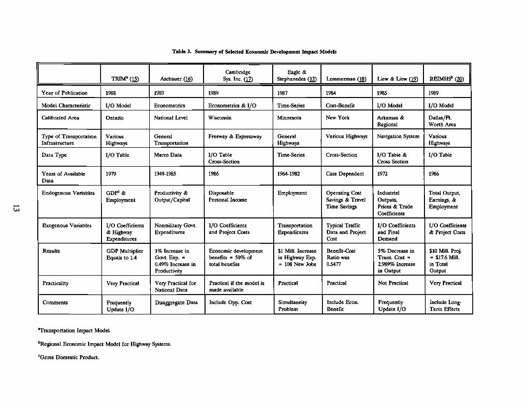
Table 3. Summary of Selected Economic Development Impact Models

Cambridge Eagle & --~ TRIM' (ll) Aschaucr CW Sys. Inc. (11) Stcphancdcs (ll) Lcmmcrman (1§) Liew & Liew (12)

Y car of Publication 1988 1989 1989 1987 1984 1985 1989

Model Characteristic 1/0 Model Econometrics Econometrics & 1/0 Time-Series Cost-Benefit 1/0 Model 1/0 Model

Calibrated Arca Ontario National Level Wisconsin Minnesota New York Arkansas & Dallas/Ft. Regional Worth Arca

Type of Transportation Various General Freeway & Expressway General Various Highways Navigation System Various Infrastructure Highways Transportation Highways Highways

Data Type 1/0 Table Macro Data 1/0 Table Time-Series Cross-Section 1/0 Table & 1/0 Table Cross-Section Cross Section

Years of Available 1979 1949-1985 1986 1964-1982 Case Dependent 1972 1986 Data

Endogenous Variables GDpc& Productivity & Disposable Employment Operating Cost Industrial Total Output, Employment Output/Capital Personal Income Savings & Travel Outputs, Earnings, &

Time Savings Prices & Trade Employment Coefficients

Exogenous Variables 1/0 Coefficients Nonmilitary Govt. 1/0 Coefficients Transportation Typical Traffic 1/0 Coefficients 1/0 Coefficients & Highway Expenditures and Project Costs Expenditures Data and Project and Final & Project Costs Expenditures Cost Demand

Results GDP Multiplier 1 % Increase in Economic development $1 Mill. Increase Benefit-Cost 5% Decrease in $10 Mill. Proj. Equals to 1.4 Govt. Exp.= benefits = 50% of in Highway Exp. Ratio was Trans. Cost = = $17.6 Mill.

0.49% Increase in total benefits = 108 New Jobs 05477 2.989% Increase in Total Productivity in Output Output

Practicality Very Practical Very Practical for Practical if the model is Practical Practical Not Practical V cry Practical National Data made available

Comments Frequently Disaggregate Data Include Opp. Cost Simultaneity Include Econ. Frequently Include Long-Update 1/0 Problem Benefit Update 1/0 Term Effects

&rransportation Impact Model

bRcgional Economic Impact Model for Highway Systems.

•oross Domestic Product.

Classes of Economic Models

A study of the relationship between transportation investment and economic development

should begin with a description of these two variables. The transportation investment can

be clearly defined as an investment that improves, maintains, or adds transportation

infrastructure. However, the concept of economic development is not universally agreed

upon. One may think of increased employment as economic development whereas others

may consider expanded total industrial output as the development of the economy. Hence,

economic development should be perceived as the total improvement of a given economy

in terms of output, employment, earnings, and standard of living of its inhabitants. An

economic model, explaining the relationship between transportation investment and

economic development, should take this information into account.

Transportation and economic development impact models can be classified according

to the following four basic forms: econometric base model, input-output base model, time­

series analysis, and cost-benefit framework. A brief summary of each of these model forms

is presented below. Table 3 provides a summary of representative examples of these models

as applied to a range of transportation improvement projects.

Econometric Models

The collection of economic theory and statistical inference is included in the econometric

base model. For example, the question of how transportation investment and economic

development relate to one another can be answered with the assistance of economic theory.

The estimation of a single equation and a system of simultaneous equations is often utilized

in order to obtain empirical results. In the past, an econometric model was capable of

analyzing only time-series or cross-section data. However, thanks to advancements in

econometric modeling, both time-series and cross-section data can be combined and

explained by the econometric method, regardless of the type of equations at hand (e.g., a

single equation or a system of equations).

14

Input-Output Models

The input-output framework has been applied in many different economic fields, ranging

from econometrics to urban planning. Input-Output (I/O) models were initially intended

to be used at the national level to analyze the interdependency among industries in an

economy; however, I/O models have been extended to cope with smaller units of the

economy. For example, regional and multiregional economic issues can be analyzed using

an I/O framework.

The I/O methodology can be separated into two major forms: simple I/O models,

variable I/O models. In simple input-output models, total outputs of all industries can be

computed from the final demand, and technical and trade coefficients, which are assumed

to be constant. This simple model is best suited for analyzing a short-term impact of policy

change. With variable I/O models, information on changes in output and input prices are

taken into consideration. Therefore, the values of the multipliers can be updated upon

receiving the price signals.

One of the more promising 1/0 models is the Regional Economic Impact Model for

Highway Systems (REIMHS), developed by Politano and Roadifer in 1988 (20). As

discussed in a previous research report (D, the REIMHS model was selected for test applications

in Texas. The REIMHS model, and the results of test applications of the model in Texas,

is discussed in detail in the subsequent chapters of this report.

Autoregressive Time-Series Analysis

The basic idea of autoregressive time-series analysis is that the future behavior of a variable

of interest will be governed by its history. The model was made famous by Box and Jenkins

(21). Autoregressive Moving Average (ARMA) and Vector Autogression (VAR) models

are parts of such analysis. The ARMA models assume that a variable in question depends

on its past values and past random errors. The VAR models, on the other hand, assume

that a column vector of the combined dependent and independent variables is a linear

15

function of a column vector of this past value and an error term. Thus, the VAR model is

capable of forecasting a column vector of variables consisting of responding variables and

driving variables.

Cost-Benefit Analysis

Most transportation projects are evaluated in terms of their costs and benefits to assist the

policy maker in identifying the most efficient project. The cost-benefit framework relies

basically on the measurement of costs and benefits of a given project. However, a good

cost-benefit analysis must take into account the importance of an opportunity cost of the

project in question. The opportunity cost is the cost of forgoing the best alternative program

in which available funds may be invested. A fundamental shortcoming of cost-benefit

analysis is that it considers only those variables which can be assigned a monetary value.

The Department currently uses a computerized Highway Economic Evaluation Model

(HEEM II) to calculate a benefit/ cost ratio for proposed highway improvement projects

(22). The HEEM II model is capable of evaluating a range of standard rural highway

improvements, as well as several special classes of highway improvement projects ( e. g., high

occupancy vehicle (HOV) projects, and two-corridor projects). However, like most benefit­

cost models, the HEEM II model does not consider economic impacts other than the direct

highway user benefits which result from highway improvement projects.

16

III. THE REGIONAL ECONOMIC IMPACT MODEL FOR HIGHWAY SYSTEMS

(REIMHS)

Overview

The overall goal of this research effort was to attempt to quantify the relationships between

expenditures for transportation improvements and economic development in Texas. This

chapter describes the basic model used to perform the preliminary analyses directed at

accomplishing this goal.

The preliminary analyses were performed using the Regional Economic Impact

Model for Highway Systems (REIMHS). As discussed in a previous report (1) published

to document the first year of this research effort, the REIMHS model was selected primarily

because it allows a more comprehensive assessment of the economic impacts of highway

investment programs than other economic evaluation models such as HEEM (22). The

REIMHS model uses data which is routinely collected by the Department or which is readily

available from widely accepted secondary sources. The REIMHS model is reasonably

tractable and is built around a fairly straightforward operating logic.

Like HEEM, the REIMHS model evaluates the following benefits associated with

highway improvements:

(1) Operating Efficiency Savings (savings in vehicle maintenance and repair costs,

oil and fuel consumption, vehicle depreciation, and tire wear);

(2) Mobility Savings (monetary value of time saved by motorists before and after

the highway improvement); and

(3) Safety Savings (accident costs before and after the improvement).

17

In addition to these three factors, the REIMHS model assesses the regional economic

impacts of highway investments. These regional economic impacts consist of the following

three components:

( 1) Estimated monetary value of all goods and services produced by the regional

industries involved in implementing the highway improvement project;

(2) Estimated monetary value resulting from the employment of workers in the

regional industries involved in implementing the highway improvement project; and

(3) Estimated total employment generated within the regional industries involved

in implementing the highway project.

The REIMHS model, then, focuses on the employment impacts of highway

investments. It does not provide estimates of the economic impacts of new land

developments or increased interregional trade flows that can result from highway

investments. The literature review (1) did not reveal any suitably tractable and/ or reliable

procedures for modeling these more comprehensive impacts of transportation investments.

It was hoped that by applying the REIMHS model in several highway corridors, a

reasonably consistent relationship between expenditures for highway improvements and

economic development would emerge. Such a relationship, if one exists, could be used by

the Department to formulate preliminary, planning-level estimates of the economic

development impact potentials of various highway improvement programs and projects.

The Regional Economic Impact Model for Highway Systems was developed by

Politano and Roadifer in 1988 (20). The main objective of the REIMHS model is to

estimate the economic impacts of investments in highway systems. Expenditures for

transportation improvements provide not only direct user benefits, such as mobility savings,

operating efficiency savings and safety savings, but direct and induced regional economic

benefits as well. The direct economic benefits consist of lower transportation costs and

18

increases in construction income, both for labor and the suppliers of construction materials.

The direct auto user benefits and the direct economic benefits can be estimated by

REIMHS provided that information concerning the cost of the project and general

transportation data are available. Additionally, the induced economic benefits of

transportation investments can also be estimated by REIMHS. The induced economic

effects are the additional economic impacts brought about by increases in spending by the

recipients of the direct economic benefits. The size of the induced economic effects, or

multiplier effects, depends on the multipliers obtained from the regional interindustry

analysis (input-output table). Using the Bureau of Economic Analysis' multipliers for

regional industrial output (~), along with employment and income estimates, REIMHS

estimates the aggregate value of the induced economic impacts in terms of industrial output

and the earnings and employment impacts of undertaking or not undertaking a given

highway project.

The REIMHS model procedures go one step farther than a conventional cost/benefit

analysis. While traditional cost/benefit analyses typically evaluate only the direct

automobile users' benefits and the project costs, the REIMHS model takes into account the

economic effects of highway investments. For example, the Highway Economic Evaluation

Model (HEEM) (22) currently used by the Department computes the present value of

benefits including safety, travel time, and operating savings and the present value of total

project costs. A benefit-cost ratio is then calculated to permit a ranking of the prospective

highway improvement projects under consideration. Furthermore, REIMHS and HEEM

share many of the same basic data sources, such as the AASHTO value of travel time and

traffic data from HPMS. With the REIMHS model, the analyst can not only rank the

prospective projects according to their benefit-cost ratios but can also evaluate projects on

the basis of their regional economic impacts.

A PC-compatible version of the REIMHS model written in MS QuickBasic has been

developed by Garcia-Diaz and Freyre (24). This interactive program requires the same data

as the original REIMHS. The PC version of REIMHS has been developed to estimate the

economic impacts of highway expenditures in each of the following five states: Arkansas,

19

Louisiana, New Mexico, Oklahoma, and Texas. Six types of highway systems can be

modeled by the PC version of the REIMHS model. These are interstate, primary, and ur­

ban highways in urban areas and interstate, primary and secondary highways in rural areas.

Data Requirements

The basic data requirements of the REIMHS model are outlined below.

1. General Transportation System Data

• Facility Type: urban interstate, urban primary, urban, rural interstate, rural

primary, and rural secondary.

• Year of Analysis.

• General Traffic Data: percentage of traffic experiencing congestion (level of

service C or worse), average annual daily vehicle of miles of travel,

percentage trucks, running speed before improvement, running speed after

improvement, number of passengers per car, fatal accidents (victims/million

veh-mi), injury accidents, property damage accidents (vehicles/million veh-mi),

and pavement condition index.

• Distribution of Vehicles: small, medium and large autos, pick-up trucks, 2A­

SU trucks, 3A-SU trucks, 2S-2 trucks, and 3S-2 trucks.

2. Project Cost Data: this information can be obtained from the FHWA Form No. 47.

• Project Type: new construction or improvement of in an existing highway.

20

• Type of Improvement: bridge widen/modify, bridge replacement, widen

traveled way, lanes added, roadway realignment, and skid resistent overlay.

• Year the project was completed.

• Project Costs: final construction cost, total cost of all materials and supplies,

final contract amount for signs, final contract amount for lighting, and total

labor cost.

• Materials Used: type, quantity and price per unit.

3. Input Industry Information (for each of the following materials):

• Chemical and petroleum refining,

• Lumber and wood products and furniture,

• Stone, clay, and glass products, and

• Primary metal industries.

Data Sources

The data required by the model on highway construction material and labor costs must be

provided by the user. It is recommended that these data be obtained from FHWA Form

No. 47. Type of highway system, project type and length of the project are also available

from this form.

The efficiency savings, consumption data for maintenance and repair, fuel, tire, oil

and depreciation costs are estimated by REIMHS using data from a 1982 FHWA-sponsored

study (25) on vehicle operating costs.

The data on running speeds needed to estimate mobility savings must be provided

by the user. These speed data are available from the Highway Performance and Monitoring

System (HPMS) Analytical Process, Version 2.1 (26).

21

The monetary value of time in the REIMHS model for both trucks and automobiles

is from the American Association of State Highway and Transportation Officials'

(AASHTO) manual on user benefits (27) [updated to represent current prices by using the

consumer price index and the wholesale price index for industrial commodities].

Data from a Federal Highway Administration (FHWA) publication, entitled

Alternative Approaches to Accident Cost Concepts: State-of-the-Art (2a), is used by

REIMHS to calculate the accident savings resulting from highway improvements.

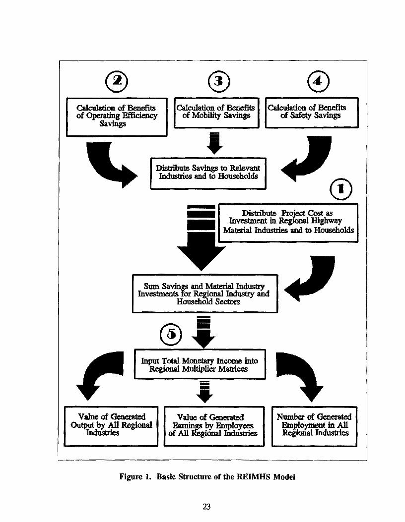
Model Structure

As shown in Figure 1, the REIMHS model consists of five basic modules as outlined below.

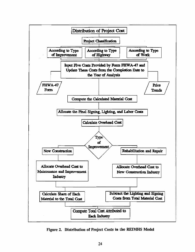
Module 1: Distribution of Project Costs. The method used by REIMHS to distribute

project costs is illustrated in Figure 2. The basic procedures used to calculate the individual

components of the project cost are outlined below.

The initial step in Module 1 is to update the five costs given in FHW A Form No.

47 from the completion date (e.g., 1980) to the year of analysis (e.g., 1986). As outlined

earlier in this chapter, the five costs are: final construction cost, labor cost, total cost of all

materials and supplies, final contract amount for signs, and final contract amount for

lighting. For example, the updated labor costs are calculated as shown below.

Labor Cost(1986) = Labor Cost(1980) x Price /ndex(1986) /Price /ndex(1980)

Where the price index is obtained from Price Trends for Federal-Aid Highway Construction

(29).

The REIMHS model also calculates the costs of the materials used in the project.

The individual material costs are calculated by simply multiplying the quantity of material

by its unit price. The total material cost is the sum of the individual material costs. Table

22

® ® © Calculation of Benefits of Operating Efficiency

Savitigs

Calculation of Benefits Calculation of Benefits of Mobility Savings of Safety Savings

ii • Distribute Savings to Relevant Indusbies and to Households

© - Dis1n"bute Project Cost as

Investment in RegiOnal Highway Material Industries and to Households

Sum Savin s and Material Industry Investments for Regional Industry and

HousehOld Sectors

--@) -Input Total Monetaty Income into

Regional Multiplie¥ Matrices

Value of Gene.med Ou~~ All Regional

InduStries

Value of Generated :Bamings by ~l~ees

of All RegiOnal Industries

Number of Generated 11--~ t in All &]mdustrles

Figure 1. Basic Structure of the REIMHS Model

23

I Distribution of Project Cost

Project Classification I

According to Type According to Type According to Type of Improvement of Highway of Wade

I l

Input Five Costs Provided by Fmm FHW A-47 and Update These Costs from the Completian Date to

the Year of Analysis

1~-41 ;=.; I Compute the Calcu1.ateQ Mated.al Cost

I Allocate the Final Signing. IJghting, and Labor Cmt8

Calculate Overhead east I

A I ~ I

I New Coostructicn I 1 Rehabilitation and Repair 1

I Allocate Oved>ead Cost to Allocate OVC'lbcad Cost to

Mainteuan~ and lmprovrmcnt New c.onstruction Industry Industry

I I

Calculate Share of Each Subtract the Lighting and Signing Mate.rial to the Total Cost Com from. Total Mat.e.tia1 Cost

I Compute Total Cost Attributed to

Bach IDdustly

Figure 2. Distribution of Project Costs in the REIMHS Model

24

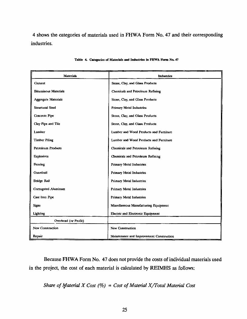
4 shows the categories of materials used in FHW A Form No. 47 and their corresponding

industries.

Table 4. Categories of Materials and Industries in FHWA Form No. 47

Materials Industries

Cement Stone, aay, and Olass Products

Bituminous Materials Chemicals and Petroleum Refining

Aggregate Materials Stone, Oay, and Glass Products

Structural Steel Primary Metal Industries

Concrete Pipe Stone, Oay, and Glass Products

aay Pipe and Tile Stone, Oay, and Glass Products

Lumber Lumber and Wood Products and Furniture

Timber Piling Lumber and Wood Products and Furniture

Petroleum Products Chemicals and Petroleum Refining

Explosives Chemicals and Petroleum Refining

Fencing Primary Metal Industries

Guarorail Primary Metal Industries

Bridge Rail Primary Metal Industries

Corrugated Aluminum Primary Metal Industries

Cast Iron Pipe Primary Metal Industries

Signs Miscellaneous Manufacturing Equipment

Lighting Electric and Electronic Equipment

Overhead (or Profit)

New Construction New Construction

Repair Maintenance and Improvement Construction

Because FHW A Form No. 4 7 does not provide the costs of individual materials used

in the project, the cost of each material is calculated by REIMHS as follows:

Share of }/aterial X Cost(%) = Cost of Material X/I'otal Material Cost

25

Material Cost (1986) = Total Material Cost (1986) - Signing Cost (1986) -

Lighting Cost (1986)

Cost of Material X = Share of Material X Cost (%) x Material. Cost

As indicated in Table 4, the total cost attributed to a given industry (e.g., Chemicals

and Petroleum Refining) is the sum of all the corresponding material costs. For example:

Total Cost = Cost of Bituminous Material + Cost of Petroleum to Petroleum

Industry Products + Cost of Explosives + Cost of Premix

Bituminous Materials to Petroleum Industry

In addition, the material cost shares by industry are calculated as:

Material Cost Share by Industry Y (%) = Total Cost of Industry Y /Final Cost(1986).

The REIMHS model assigns the overhead costs (or profit) to either the new

construction industry or the maintenance and improvement construction industry, as shown

in Table 4. This component is calculated as:

Overhead (1986) = Final Cost (1986) - Labor Cost (1986) - Total Material Cost (1986)

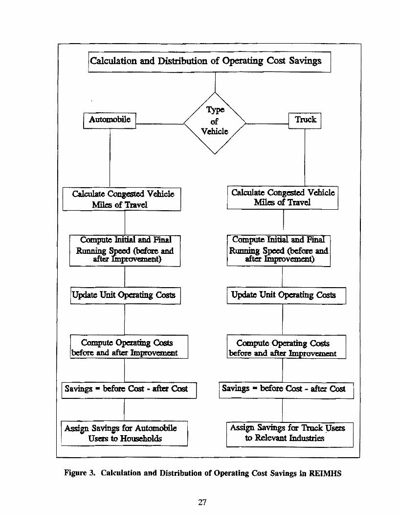
Module 2 Calculation and Distribution of Operating Efficiency Savings. The

Operating Efficiency Savings (OES) refers to the differences in maintenance and repair

costs, oil and fuel consumption, depreciation for trucks and automobiles, and tire wear

before and after the highway improvement. The OES are computed for traffic experiencing

congestion (defined as roadways with a volume to capacity ratio greater than 0.77 for all

urban roads and 0.18 for all rural roads). These changes translate into savings in vehicle

operating costs. Such savings realized by households and relevant industries are assumed

to be spent in the regional economy. Figure 3 outlines the procedure used in REIMHS to

calculate OES. The OES for automobile users are allocated to the households, while OES

26

Calculation and Distribution of Operating Cost Savings

Type I Automobile ! of ! Truck j

Vehicle

Calculate Congested V ehiele CalcuJate Congested Vehicle Mil.es of Travel Mi1c'8 of Travel

Compute Initial and Final Compute Initial and Final

Rlmn~S==)and Running Speed (before and after Il'llprovement)

Update Unit Operating ~ Update Unit Operating Co,,1s

Compute Operating Costs Compute Operating CoSs before and after Improvement before and afttt Improvement

Savings • before Cost - after Call I I Savings - before Cost - after Cost

Assign Savinss for Automobile A.smgn Savings for Truck :Users Usets to Households to Relevant Industries

Figure 3. Calculation and Distribution of Operating Cost Savings in REIMHS

27

for trucks is assigned to the corresponding industries. Data from the 1982 Census of

Transportation: Truck lnventozy and Use Survey. United States(J,Q) is used to calculate truck

vehicle-miles of travel for various trip purposes and to calculate the percentage of truck

vehicle-miles of travel for each industry. The OES are then allocated to the relevant

industries by the percentage of truck vehicle-miles of travel for those industries.

Module 3. Calculation and Distribution of Mobility Savings. The Mobility Savings

(MS) is the monetary value of time saved after the improvement by traffic which

experienced congestion before the highway improvement. The MS calculation procedures

performed by REIMHS are depicted in Figure 4. The value of time saved refers to the

difference between the average running speed before and after the improvement. The

MSHTO Manual on User Benefits of Highway and Bus-Transit Improvements (21)

provides the values of time used in REIMHS ($8.20/hour for automobiles and $13.98/hour

for trucks). The MS for automobile users are allocated to the households and the MS for

trucks are distributed among the relevant industries as described in Module 2 (Calculation

and Distribution of Operating Efficiency Savings).

Module 4. Calculation and Distribution of Safety Savings. The Safety Savings (SS) of

motor vehicles are the differences between the accident costs before and after the roadway

improvement. The SS are computed by REIMHS as summarized in Figure 5. The accident

costs are separated into fatal, injury, and property damage costs. Ten percent (10%) of the

total SS are assigned to households, and 90% of the savings are assigned to the insurance

industry.

Module 5. Calculation of Regional Economic Impacts. The estimated Regional

Economic Impacts (REI) can be disaggregated into three components: total estimated

monetary value of all goods and services produced by the regional industries, total estimated

monetary value of all workers employed by the regional industries, and total estimated

employment generated within the regional industries. These estimates are calculated by first

summing all the investments calculated in Module 1 and all the savings from Modules 2 -

4 for each industry in the region. Second, the total investments and savings available in

28

Mobility or Travel Time Savings-

Automobile --------<

Savings for Autos

for a Change from

Congested and Normal

Conditions to Ftee Flow

Compute Net Mobility Savings

for Automobile Users by

Subtracting Mobility Savings of

Normal to Free Flow from

Congested to Pree Plow

Assign Savings for Automobile

Users to Households

Type of

Vehicle

Savings for Trucks

for a Change from

Congested and Normal

Conditions to Free Flow

Compute Net Mobility Savings

for Truck Use.rs by

Subtracting Mobility Savings of

Normal to Free Flow from

Congested to Ptee Plow

Amgn Savings for Truck Users

to Relevant Industries

Figure 4. Calculation and Distribution of Mobility Savings in REIMHS

29

Safety Savings

Determine the Direct Costs for Fatal. InjuryJ

and Propeity Damage only Accidents

Compute the V chicle t.fi.1.es of Travel

for the lfighway System

Calculate the Rate of Occutre11ce for

Three Types af Accidents

Determine the Accident Reduction Factors

for Three Types of Accidents, for Bach Type

of mgb.way Improvement

I Calculate the Total Safety Savings

I 10% of the Total Safety Savings

Goes to Hou.;eb.olds

90% of the Total Safety Savings

Goes to the Imurattce Ittdustry

Figure 5. Calculation and Distribution of Safety Savings in REIMHS

30

each industry are represented as a row vector. Then, the Bureau of Economic Analysis'

multipliers for all regional industrial output (23.), earnings of employees in all industries, and

employment (which are available in column vector forms) are used to compute the REI as

illustrated in the following example. Earnings and employment effects are calculated in a

similar manner.

Total Investment and Savings

Industry 1

[ 100

Industry 2

200]

Previous Applications in Texas

x

Output Multipliers = Output Effects

Industry 1 [ 1.5 ]

Industry 2 1.8

( 1OOx1.5) + (200x 1.8)

= $510

A case study application of the REIMHS model in a 16-county area surrounding Dallas/Fort

Worth was performed by Politano and Roadifer in 1989 (20). Their study evaluated the

impacts of a $10 million highway improvement project. As shown in Table 5, the average

benefits over several types of improvements resulting from efficiency, mobility, and safety

savings (or losses) were estimated to be $0.13 million, $1.05 million, and $0.50 million,

respectively for urban areas, and -$0.01 million, $0.10 million, and $0.03 million, respectively

for rural areas. Total direct highway user benefits were estimated to be $1.68 million for

urban areas and $0.13 million for rural areas. In addition, the REIMHS model estimated

that this investment would generate $16.08 million and $4.56 million in total regional output

and total regional earnings, respectively for urban areas, and $17.22 million and $4.43

million in total regional output and earnings, respectively for rural areas.

Area Type

Urban

Rural

Table 5. Impacts of a $19 Million Highway Imp~nt lnvesbnent on Dallas/Fort Wortll Region as Reported by Po6tano and Roadifer

Average Average Average Average Average Average Efficiency Mobility Safety Output Earnings Employment

($Millions) ($Millions) ($Millions) ($Millions) (S Millions) (Jobs)

0.1328 1.048 0.502 16.08 4.56 202

-0.0054 0.104 0.0317 17.22 4.43 194

Souree: Reference 20 and authors' calculations.

31

Benefit-Cost Ratio

1.61

1.72

The results of the Politano and Roadifer study indicate that every $1 invested in

highway improvements produces an estimated $1.61 and $1.72 in total regional output for

urban and rural areas, respectively. Also, the $10 million highway investment would create

a total of nearly 400 jobs (an average of 202 urban jobs and 194 rural jobs).

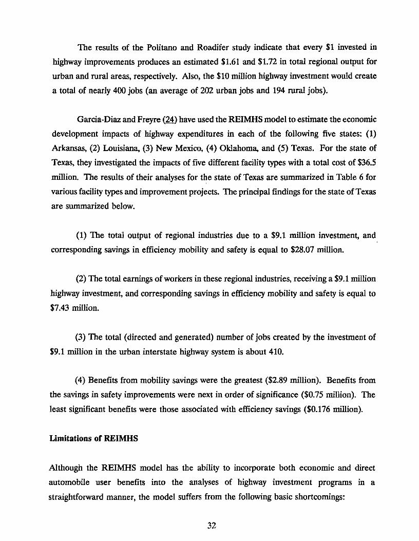
Garcia-Diaz and Freyre (24) have used the REIMHS model to estimate the economic

development impacts of highway expenditures in each of the following five states: (1)

Arkansas, (2) Louisiana, (3) New Mexico, (4) Oklahoma, and (5) Texas. For the state of

Texas, they investigated the impacts of five different facility types with a total cost of $36.5

million. The results of their analyses for the state of Texas are summarized in Table 6 for

various facility types and improvement projects. The principal findings for the state of Texas

are summarized below.

(1) The total output of regional industries due to a $9.1 million investment, and

corresponding savings in efficiency mobility and safety is equal to $28.07 million.

(2) The total earnings of workers in these regional industries, receiving a $9.1 million

highway investment, and corresponding savings in efficiency mobility and safety is equal to

$7.43 million.

(3) The total (directed and generated) number of jobs created by the investment of

$9.1 million in the urban interstate highway system is about 410.

(4) Benefits from mobility savings were the greatest ($2.89 million). Benefits from

the savings in safety improvements were next in order of significance ($0.75 million). The

least significant benefits were those associated with efficiency savings ($0.176 million).

Limitations of REIMHS

Although the REIMHS model has the ability to incorporate both economic and direct

automobile user benefits into the analyses of highway investment programs in a

straightforward manner, the model suffers from the following basic shortcomings:

32

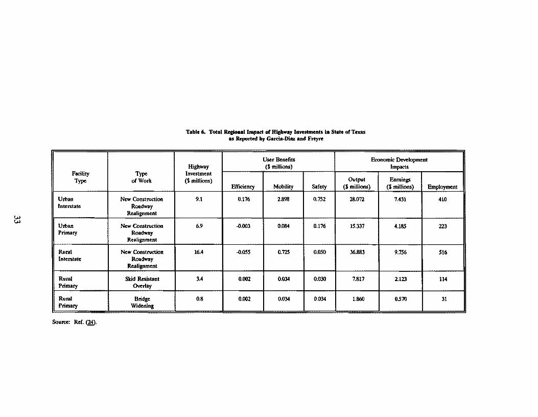
Facility Type Type of Work

Urban New Construction Interstate Roadway

Realignment

Urban New Construction Primary Roadway

Realignment

Rural New Construction Interstate Roadway

Realignment

Rural Skid Resistant Primary Overlay

Rural Bridge Primary Widening

Source: Ref. (ID.

Table 6. Total Regional Impact of Highway Investments in State of Texas as Reported by Gan:ia·Diaz and Freyre

User Benefits Highway ($ millions)

Investment ($ millions) Output

Efficiency Mobility Safety ($ millions)

9.1 0.176 2.898 0.752 28.072

6.9 -0.003 0.084 0.176 15.337

16.4 -0.0SS 0.725 o.oso 36.883

3.4 0.002 0.034 0.030 7.817

0.8 0.002 0.034 0.034 1.860

Economic Development Impacts

Earnings ($ millions) Employment

7.431 410

4.185 223

9.756 516

2.123 114

0.570 31

( 1) The REIMHS model cannot be used to evaluate a proposed highway

improvement project. This is because the project cost data required by REIMHS is

available only after the completion of the project (e.g., from FHW A Form-47).

(2) REIMHS does not take into account the length of the project in calculating the

direct user benefits attributable to safety savings, operating cost savings, and travel time

savings -- each of which directly depends on the length of the highway construction project.

(3) Because most highway improvements have a long life, the benefits (at least

the direct user benefits) resulting from these improvements should be computed over the

entire life of the project and represented in terms of the discounted present value of the

costs and benefits. This option is not currently available in the REIMHS model. The

HEEM model, on the other hand, computes the discounted present value of the stream of

user benefits and costs over the life of the improvement.

( 4) The structure of the current REIMHS program makes it difficult to update

the key variables in the model (e.g., to use data from other sources that are updated on a

regular basis).

In an attempt to remedy these basic shortcomings, a Modified Regional Economic

Impact Model for Highway Systems (MREIMHS) was developed and tested as part of this

research effort. The basic structure of the current REIMHS model was retained. However,

in MREIMHS the distribution of the cost of highway construction projects is calculated

using data from Hi~hway Statistics (J.l). The data in Hiiiihway Statistics is frequently

updated and can be easily incorporated into MREIMHS. Finally, by combining the Highway

Statistics data with the (discounted) direct user benefits available from HEEM, the

MREIMHS model can calculate regional economic impacts as well as the benefit-cost ratio

of proposed highway investment programs.

The proposed MREIMHS model is described in detail in the following sections of

this chapter. The results of a preliminary test application of the MREIMHS model in an

34

intercity highway corridor in Texas are presented in the following chapter of this research

report.

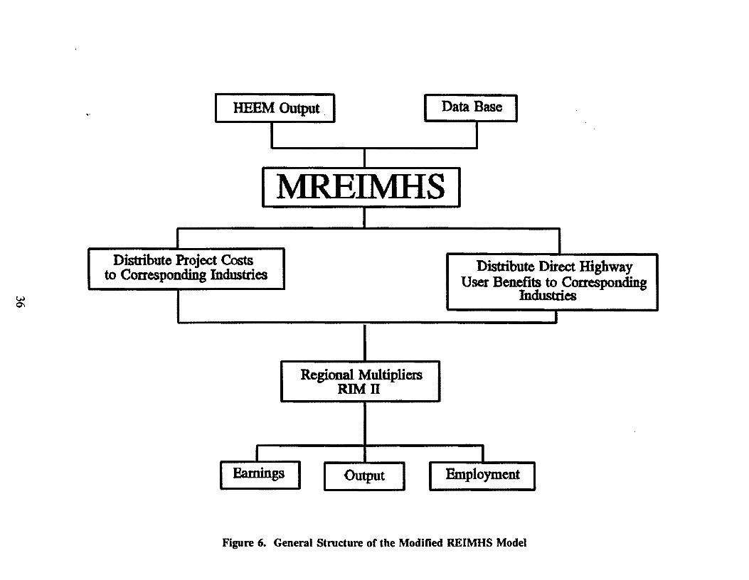
The Modified REIMHS Model

The MREIMHS has been designed to extend the basic REIMHS model to permit the

evaluation of proposed highway improvement projects in terms of their contributions to the

regional economy. The general structure of MREIMHS is shown in Figure 6. The

MREIMHS utilizes the output from an existing computerized cost-benefit model (HEEM),

which is currently employed by TxDOT to rank proposed highway projects. The MREIMHS

model uses annual project cost information from Hi~way Statistics (31) and the direct user

benefits from the HEEM model to estimate the regional economic impacts of proposed

highway investments. The results of the MREIMHS model can be used to calculate a

benefit-cost ratio which can then be used to rank highway projects. The key components

of the MREIMHS model are described in the following subsections of this chapter.

Distribution of Project Costs in MREIMHS

Table 7 presents a general summary of the annual construction cost data contained in

Hi~hway Statistics (J,1). The MREIMHS model assigns the total construction cost to the

following nine industries:

1. new construction,

2. repair and maintenance construction,

3. primary metal industry,

4. stone, clay, and glass products,

5. petroleum refining industry,

6. lumber, wood, and furniture products,

7. electric and electronic equipment,

8. miscellaneous manufacturing, and

9. households.

35

HEEM Output . Data Base

MREIMHS

Distribute Project Costs to Conesponding Industries

Earnings

Regional Multipliers RIM II

Output

Distribute Direct mghway User Benefits to Conesponding

Industries I

I Employment

Figure 6. General Structure of the Modified REIMHS Model

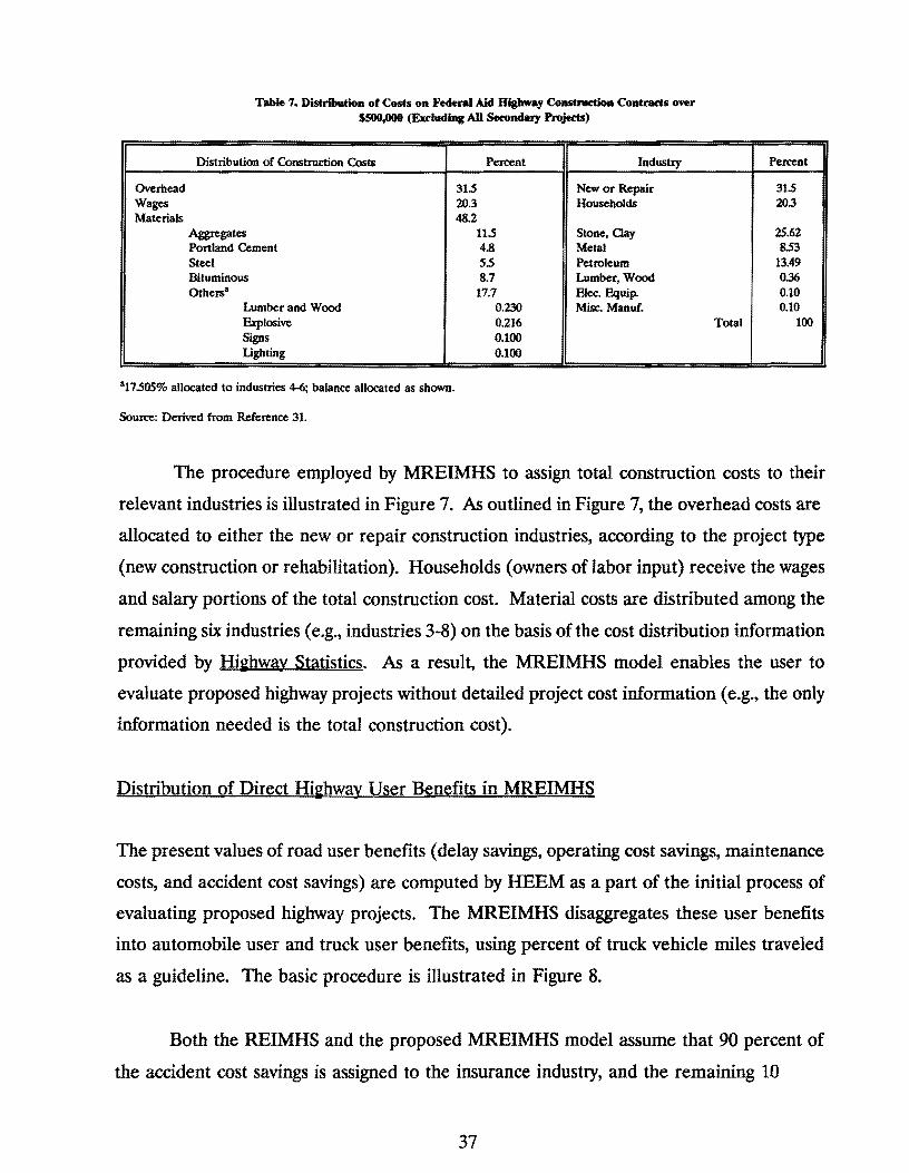
Table 7. Distribution of Costs on Federal Aid Highway Construction Contracts over $500,000 (Exdudina All Secondary Projects)

Distribution of Construction Costs Percent Industty

Overhead 31.5 New or Repair Wages 20.3 Households Materials 48.2

Aggregates 11.5 Stone, Clay Portland Cement 4.8 Metal Steel S.5 Petroleum Bituminous 8.7 Lumber, Wood Other.s• 17.7 Elec. Equip.

Lumber and Wood 0.230 Misc. Manuf. Explosive 0.216 Signs 0.100 Lighting 0.100

•17.505% allocated to industries 4-6; balance allocated as shown.

Source: Derived from Reference 31.

Percent

31.5 20.3

25.62 8.53

13.49 0.36 0.10 0.10

Total 100

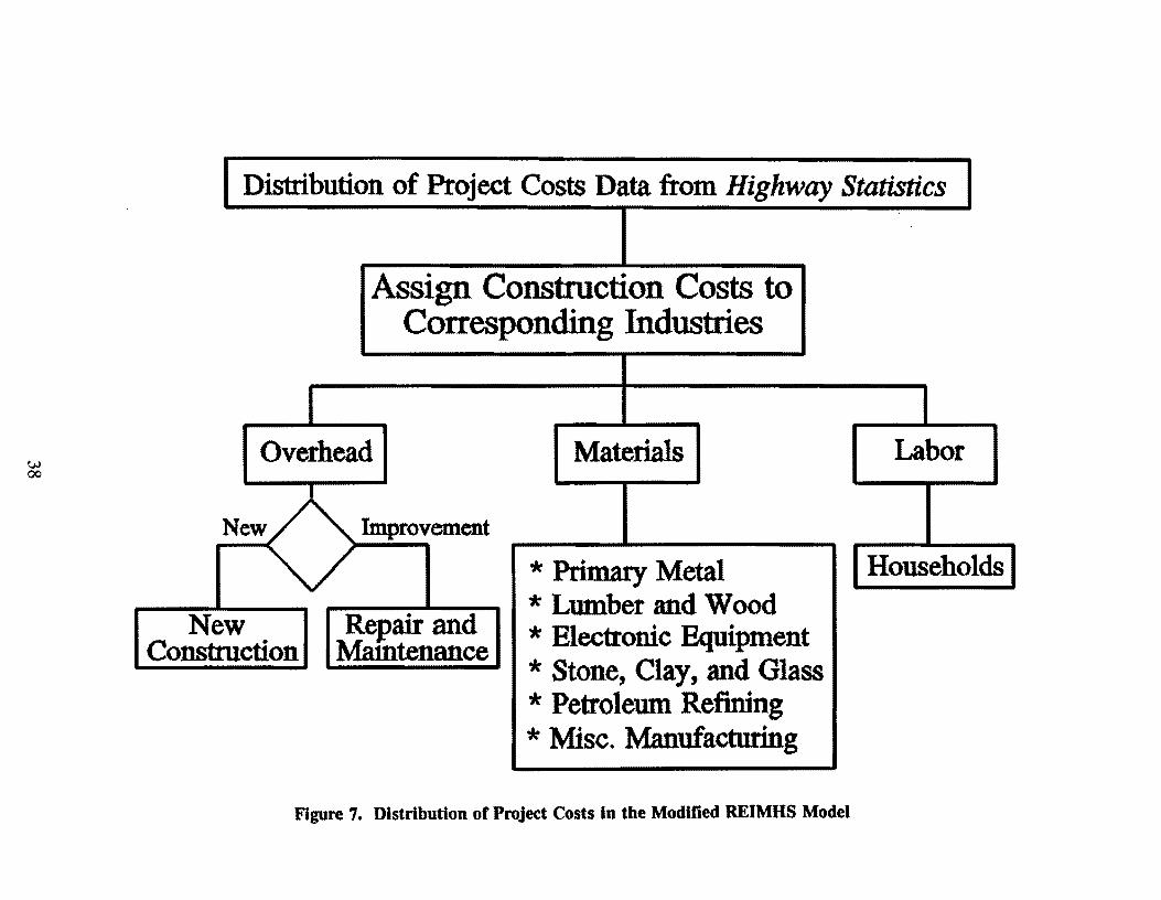
The procedure employed by MREIMHS to assign total construction costs to their

relevant industries is illustrated in Figure 7. As outlined in Figure 7, the overhead costs are

allocated to either the new or repair construction industries, according to the project type

(new construction or rehabilitation). Households (owners of labor input) receive the wages

and salary portions of the total construction cost. Material costs are distributed among the

remaining six industries (e.g., industries 3-8) on the basis of the cost distribution information

provided by Highway Statistics. As a result, the MREIMHS model enables the user to

evaluate proposed highway projects without detailed project cost information (e.g., the only

information needed is the total construction cost).

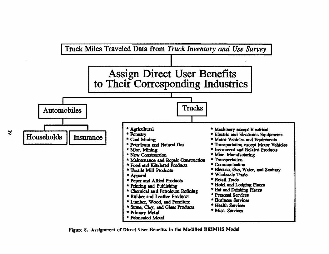
Distribution of Direct Highway User Benefits in MREIMHS

The present values of road user benefits (delay savings, operating cost savings, maintenance

costs, and accident cost savings) are computed by HEEM as a part of the initial process of

evaluating proposed highway projects. The MREIMHS disaggregates these user benefits

into automobile user and truck user benefits, using percent of truck vehicle miles traveled

as a guideline. The basic procedure is illustrated in Figure 8.

Both the REIMHS and the proposed MREIMHS model assume that 90 percent of

the accident cost savings is assigned to the insurance industry, and the remaining 10

37

w 00

Distribution of Project Costs Data from Highway Statistics

Assign Construction Costs to Corresponding Industries

I Overhead

New A Improvement

New Repair and Construction Mamtenance

Materials

* Primary Metal * Lumber and Wood * Electronic Equipment *Stone, Clay, and Glass * Petroleum Refining * Misc. Manufacturing

Figure 7. Distribution of Project Costs in the Modified REIMHS Model

Labor

Households

I Truck Miles Traveled Data from Truck Inventory and Use Survey I

I Automobiles

I I I

Assign Direct User Benefits to Their Corresponding Industries

I I

Trucks I

* Machinery except Bledrica1

Households Insurance • Agricultural •Forestry * o.IMining

* Blr.drlc and B1ecttonic Equipments * M.otor Vehicles and Eqafp1ats

* PcttoJcum ml Natural Gas * Misc. Minina • New O:mmuction * Maintenance and Repair Construction * Food and Kindcred Products * Textile Mill Producis • Apparel * Paper and Allied Produds * Printing and Publishing * Olemical an.d Petroleum Refining * Rubber and l.eafber Products * Lumber. Wood. and Pomiture * Stonc, Clay. and Glau Products • Primary Metal * Fabricated Metal

* Transportation CKept Matar Vrllicb * Imtrumtot and Related Producta * Misc. Manufacturing * Transportation * Communicatim * B1ectric, ~ Water, and Sanitary * Wholesale Trade * Retail Ttadc * Hotd and Lodging P1aa:s * Bat and J)rinldng P1a.cca *Persaoal~ * Business Services * Health Services * Misc. Services

Figure 8. Assignment of Direct User Benefits in the Modified REIMHS Model

percent is assigned to households. The sum of operating cost savings, maintenance costs

(negative or positive), and delay time savings for automobile users is allocated to the

households.

The total truck user benefits are distributed to their corresponding industries

according to the percent of truck miles in each industry. The required truck travel data are

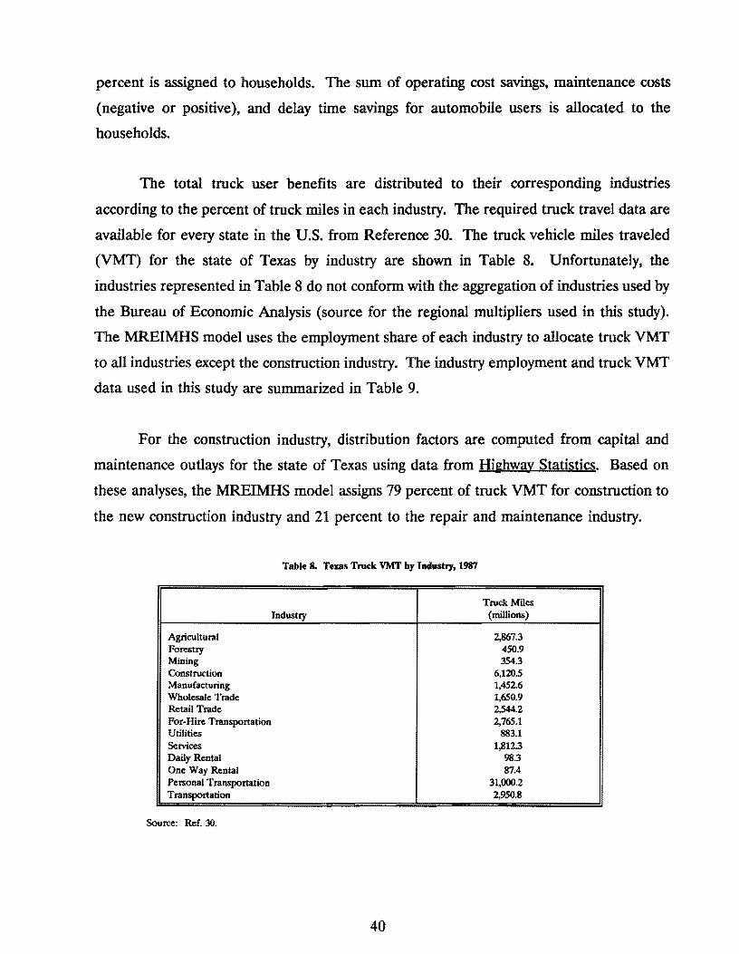
available for every state in the U.S. from Reference 30. The truck vehicle miles traveled

(VMT) for the state of Texas by industry are shown in Table 8. Unfortunately, the

industries represented in Table 8 do not conform with the aggregation of industries used by

the Bureau of Economic Analysis (source for the regional multipliers used in this study).

The MREIMHS model uses the employment share of each industry to allocate truck VMT

to all industries except the construction industry. The industry employment and truck VMT

data used in this study are summarized in Table 9.

For the construction industry, distribution factors are computed from capital and

maintenance outlays for the state of Texas using data from Hi~hway Statistics. Based on

these analyses, the MREIMHS model assigns 79 percent of truck VMT for construction to

the new construction industry and 21 percent to the repair and maintenance industry.

Table 8. Texas Truck VMT by Industry, 1'87

Truck Miles Industry (millions)

Agricultural 2,867.3 Forestry 450.9 Mining 354.3 Construction 6,120.5 Manufacturing 1,452.6 Wholesale Trade 1,650.9 Retail Trade 2,544.2 For-Hire Transportation 2,765.1 Utilities 883.1 Services 1,BU.3 Daily Rental 98.3 One Way Rental 87.4 Personal Transportation 31,000.2 Transportation 2,950.8

Source: Ref. 30.

40

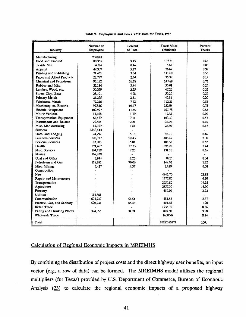
Table 9. Employment and Truck VMT Data for Texas, 1987

Number of Percent Truck Miles Percent Industry Employees of Total (Millions) Trucks

Manufacturing 934,841 Food and Kindred 88,36.5 9.45 137.31 0.68 Textile Mill 4,262 0.46 6.62 0.03 Apparel 49,307 5.27 76.62 0.38 Printing and Publishing 71,451 7.64 111.02 0.55 Paper and Allied Products 22,m 2.44 35.39 0.17 Chemical and Petroleum 95,172 10.18 147.88 0.73 Rubber and Misc. 32,184 3.44 50.01 0.25 Lumber, Wood, etc. 30,379 3.25 47.20 0.23 Stone, Clay,Cilass 38,101 4.08 59.20 0.29 Primary Metals 26,295 2.81 40.86 0.20 Fabricated Metals 72,216 7.72 112.21 0.55 Machinery, ex. Electric 97,846 10.47 152.04 0.75 Electric Equipment 107,977 11.55 167.78 0.83 Motor Vehicles 11,168 1.19 17.35 0.09 Transportation Equipment 66,479 7.11 103.30 051 Instruments and Related 20,655 2.21 32.09 0.16 Misc. Manufacturing 15,059 1.61 23.40 0.12 Services 1,443,412 - - -Hotel and Lodging 74,792 5.18 93.91 0.46 Business Services 323,737 22.43 406.47 2.00 Personal Services 83,883 5.81 105.32 0.52 Health 394,467 27.33 395.28 2.44 Misc. Services 104,418 7.23 131.10 0.65 Mining 169,828 - - -Coal and Other 3,844 2.26 8.02 0.04 Petroleum and Cias 118,882 70.00 248.02 1.22 Misc. Mining 7,427 4.37 15.49 0.08 Construction - - - -New - - 4842.70 23.88 Repair and Maintenance - - 1277.80 6.30 Transportation - - 2950.80 14.55 Agriculture - - 2857.30 14.09 Forestry . . 450.90 2.22 Utilities 114,861 - - -Communication 624,927 5454 481.62 2.37 Electric, Gas, and Sanitary 520,934 45.46 401.48 1.98 Retail Trade - - 1736.70 8.56 Eating and Drinking Places 394,055 31.74 807.50 3.98 Wholesale Trade 1650.90 8.14

Total 20282.60572 100.

Calculation of Regional Economic Impacts in MREIMHS

By combining the distribution of project costs and the direct highway user benefits, an input

vector (e.g., a row of data) can be formed. The MREIMHS model utilizes the regional

multipliers (for Texas) provided by U.S. Department of Commerce, Bureau of Economic

Analysis (23) to calculate the regional economic impacts of a proposed highway

41

improvement project. The economic impacts include the value of total changes in regional

output, the earnings that regional industries pay to households, and the number of jobs that

regional industries provide. By multiplying the input vector by the regional multipliers

matrix, the regional economic impacts resulting from investment in a highway improvement

project are obtained.

42

IV. PRELIMINARY ANALYSIS OF ECONOMIC IMPACTS OF HIGHWAY

EXPENDITURES IN TEXAS

Overview

This chapter presents the results of a preliminary, test application of the MREIMHS model

in an intercity highway corridor in Texas. The scope of this investigation should be viewed

as exploratory and, therefore, preliminary in nature, as the findings are based on test

applications in a single highway corridor~ The results do, however, indicate that the

economic development impacts of highway investments can be substantial and that

additional research and model testing should be pursued by the Department.

Study Corridor

The Pinehurst corridor (Figure 9) was selected for the sample application of the modified

REIMHS model in Texas. This corridor is situated northwest of the greater Houston area

between U.S. Highway 290 and Interstate Highway 45 and is one of the most rapidly

developing areas in Harris and Montgomery Counties. According to 1980 census data,

Montgomery County experienced a 160 percent increase in population during the 1970s.

Land use within the general highway corridor between Pinehurst and Houston is

closely associated with the economic characteristics of the area. Land use is divided

primarily between the economic interest of agriculture, mineral production, and

residential/ commercial/industrial development. The residential/ commercial/industrial

development in this corridor is located within and adjacent to the larger cities. Examples

include a research and development center located in the Woodlands and the new Compaq

computer plant near Tomball.

The economy of this corridor is based on agriculture, mineral production, tourism,

and a wide range of manufacturing activities. Additionally, this corridor has the potential

to become a new "high-tech" research and development area within the state.

43

Figure 9. Bryan-College Station to Pinehurst Study Area

44

The Department has used the HEEM model to evaluate the direct w;er benefits

resulting from a number of new highway improvements in the study corridor. The

Department's analyses focused specifically on the feasibility of a new roadway in the

corridor. The new roadway would follow State Highway (SH) 6 from Bryan-College Station

to approximately 2.9 miles south of Navasota. From this point, the route would follow a

new southeastwardly alignment across Grimes County, north of Todd Mission, into

Montgomery County, north of Magnolia, and intersect Farm to Market (FM) Road 1774 and

SH 249 just south of Pinehurst. The proposed route includes approximately 26.9 miles of

SH 6 and approximately 26.5 miles on a new alignment.

The Department evaluated the following three highway improvement alternatives

(~):

(1) A four-lane freeway along the proposed new alignment with the necessary

right-of-way (ROW) acquired in accordance with Departmental policies.

(2) A four-lane freeway along the proposed new alignment with partial donation

of the necessary ROW.

(3) Upgrade existing roadways in the corridor to four-lane freeways.

The estimated total costs (construction plus ROW) for alternatives 1, 2, and 3 are

$163.3 million, $125.9 million, and $167.4 million, respectively (32).

Summary of Test Application of the Modified REIMHS Model

The modified REIMHS model was ~sed to estimate the economic development impacts of

the three improvement alternatives described in the previous section of this chapter. The

results of the test application of MREIMHS in the Pinehurst Corridor are shown in Table

10. The results of the preliminary analyses in the Pinehurst corridor indicate that the that

each of the highway investment alternatives would bring approximately $200 million of total

45

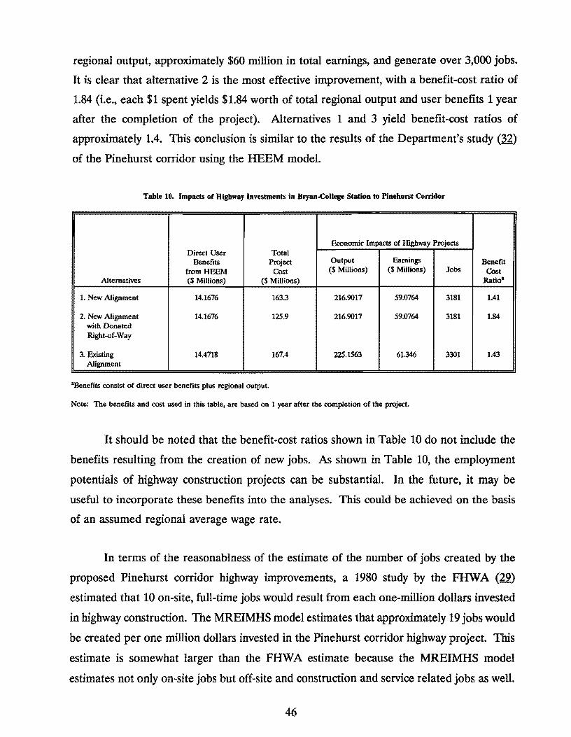
regional output, approximately $60 million in total earnings, and generate over 3,000 jobs.

It is clear that alternative 2 is the most effective improvement, with a benefit-cost ratio of

1.84 (i.e., each $1 spent yields $1.84 worth of total regional output and user benefits 1 year

after the completion of the project). Alternatives 1 and 3 yield benefit-cost ratios of

approximately 1.4. This conclusion is similar to the results of the Department's study (:12)

of the Pinehurst corridor using the HEEM model.

Table 10. Impacts or Highway Investments in Bryan.College Station to Pinehurst Corridor

Economic Impacts of Highway Projects Direct User Total

Benefits Project Output Earnings Benefit from HEEM Cost ($Millions) ($Millions) Jobs Cost

Alternatives ($Millions) ($Millions) Ratio•

1. New Alignment 14.1676 163.3 216.9017 59.0764 3181 1.41

2. New Alignment 14.1676 125.9 216.9017 59.0764 3181 1.84 with Donated Right-of-Way

3. Existing 14.4718 167.4 225.1563 61.346 3301 1.43 Alignment

•Benefits consist of direct user benefits plus regional output.

Note: The benefits and cost used in this table, are based on 1 year after the completion of the project.

It should be noted that the benefit-cost ratios shown in Table 10 do not include the

benefits resulting from the creation of new jobs. As shown in Table 10, the employment

potentials of highway construction projects can be substantial. In the future, it may be

useful to incorporate these benefits into the analyses. This could be achieved on the basis

of an assumed regional average wage rate.

In terms of the reasonablness of the estimate of the number of jobs created by the

proposed Pinehurst corridor highway improvements, a 1980 study by the FHWA (29)

estimated that 10 on-site, full-time jobs would result from each one-million dollars invested

in highway construction. The MREIMHS model estimates that approximately 19 jobs would

be created per one million dollars invested in the Pinehurst corridor highway project. This

estimate is somewhat larger than the FHW A estimate because the MREIMHS model

estimates not only on-site jobs but off-site and construction and service related jobs as well.

46

A Bureau of Labor Statistics study (~) reported that for each million dollars invested

in highway construction generates an average of 22 new jobs. Similarly, Politano and

Roadifer (2.Q) have estimated that each one million dollar investment in highway

construction results in from 16 to 23 new jobs. Garcia-Diaz and Freyre (24) estimate a

somewhat higher job creation rate of from 28 to 45 new jobs per million dollars invested in

highway construction. The number of jobs estimated by the MREIMHS model, then,

appears to comparable to the findings of other studies.

47

48

V. CONCLUSIONS AND RECOMMENDATIONS

Conclusions

Public investment, economic development, and their relationship have long been recognized

as important economic issues. In recent years, there has been a flurry of research directed

at addressing the question of how economic development and transportation investment are

related to each other. There appears to be a general consensus that ample, well maintained

highways, streets, and roads are important to an area's development potential. However,

due to a variety of external factors, there is considerable controversy concerning the precise

nature of the linkage between transportation improvements and economic development.

Some of the external factors which complicate an understanding of this linkage include

availability and cost of land, labor, and capital; relative tax rates; environmental and general

quality of life; and the presence of needed services and other types of infrastructure. In

short, it appears that good transportation is a necessary but not sufficient condition for

economic development to occur.

The results of this investigation of the relationship between economic development

and expenditures for transportation improvements indicate that while the economic benefits

can be substantial, additional research will be needed to quantify the precise nature of this

relationship. Despite the uncertainty concerning the nature of the relationship between

transportation and economic development, many states consider the economic development

impacts of expenditures for transportation facilities and services in the development of

transportation improvement programs. Specifically, 36 states explicitly consider economic

development potentials in their highway programming activities. Of these states, 14

(including Texas) incorporate economic development objectives into the programming

process but do not have special transportation funds or programs for the specific purpose

of fostering economic development. The remaining 22 states have categorical funding or

bonding authority for transportation improvements which is intended to promote economic

49

development. Because most of these economic development programs are relatively new,

data on the impacts of these programs are extremely limited.

As more and more states institute programs to increase the effectiveness of

transportation improvement programs, it appears likely that the economic development

potentials of various transportation investment options will become increasingly important.

Consequently, there is a need to quantify the potential economic development impacts of

transportation improvements, and to identify those situations which are most likely to benefit

from investments in new or expanded transportation facilities and services. The following

section of this chapter presents several general recommendations for achieving these ends

in Texas.

Recommendations

The recommendations drawn from this research project are presented in the following

subsections of this chapter. The recommendations focus on the following aspects of this

research topic area: (1) preliminary guidelines concerning the economic development

impacts of expenditures for state highway improvements; (2) additional refinement and

testing of the modified REIMHS model; and (3) future research the Department should

conduct and/or sponsor in the area of transportation and economic development.

Economic Development Impact Guidelines

A summary of the economic development impacts of expenditures for transportation

improvements, as estimated as part of this research effort and by other researchers, is

presented in Table 11. As indicated by the limited data summarized in Table 11, economic

development benefits as a percent of total benefits range from a low of 48 percent to a high

of 98 percent. Based on these limited data, it does not appear to be unreasonable to assume

that the monetary value of the economic development benefits resulting from highway

investments are at least equal to the direct user benefits which have traditionally been the focus

50

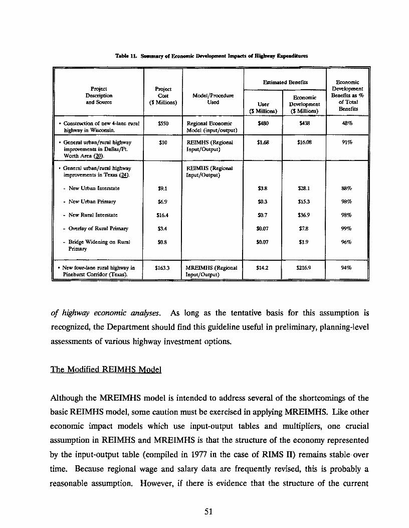
Table lL Summary of Economic Development Impacts of Highway Expenditures

Estimated Benefits Economic Project Project Development

Description Cost Model/Procedure Economic Benefits as % and Source ($ Millions) Used User Development of Total

($Millions) ($ Millions) Benefits

• Construction of new 4-lane rural 1550 Regional Economic $480 $438 48% highway in Wisconsin. Model (input/output)

• General urban/rural highway $10 REIMHS (Regional $1.68 $16.08 91% improvements in Dallas/Ft. Input/Output) Worth Area QID.

• General urban/rural highway REIMHS (Regional improvements in Texas (W. Input/Output)

- New Urban Interstate $9.1 $3.8 $28.1 88%

- New Urban Primary $6.9 $0.3 $15.3 98%

- New Rural Interstate $16.4 $0.7 $36.9 98%

- Overlay of Rural Primary $3.4 $0.07 $7.8 99%

- Bridge Widening on Rural $0.8 $0.07 $1.9 96% Primary

• New four-lane rural highway in $163.3 MREIMHS (Regional $14.2 $216.9 94% Pinehurst Corridor (Texas). Input/Output)

of highway economic analyses. As long as the tentative basis for this assumption is

recognized, the Department should find this guideline useful in preliminary, planning-level

assessments of various highway investment options.

The Modified REIMHS Model

Although the MREIMHS model is intended to address several of the shortcomings of the

basic REIMHS model, some caution must be exercised in applying MREIMHS. Like other

economic impact models which use input-output tables and multipliers, one crucial

assumption in REIMHS and MREIMHS is that the structure of the economy represented

by the input-output table (compiled in 1977 in the case of RIMS 11) remains stable over

time. Because regional wage and salary data are frequently revised, this is probably a

reasonable assumption. However, if there is evidence that the structure of the current

51

regional economy differs substantially from the structure represented by the input-output

tables, the results from REIMHS, MREIMHS or other economic impact models should be

used with caution.

None of the existing economic development impact models and techniques reviewed

in this study explicitly takes into account the costs of right-of-way acquisition. In many

cases, these costs can be substantial. Future versions of the MREIMHS model should

incorporate right-of-way costs into the analysis.

The MREIMHS model incorporates the results (e.g., direct highway user benefits)

computed by HEEM. The HEEM model has recently undergone a critical reevaluation by

TTI researchers. It has been shown that some key assumptions in HEEM should be

updated and revised; thus, HEEM II (a revised version of HEEM) has been developed.

The improved procedures in HEEM II for estimating direct highway user benefits should

be incorporated into subsequent versions of MREIMHS.

It is the recommendation of this study that the revisions outlined above should be

incorporated into the MREIMHS model. The MREIMHS model should then be tested in

additional highway corridors in Texas. Following the implementation and testing of these

revisions, the appropriate Department personnel should be trained in the maintenance and

application of the MREIMHS model. Such a program would be similar to current training

programs concerning the Department's use of the HEEM model.

Future Research

The Department's future research efforts should focus on the following three general aspects

of the relationship between transportation and economic development: (1) quantification

of the economic development potentials of various transportation investment programs; (2)

identification of the physical, economic, and sociodemographic environments in which

investments in transportation facilities and services offer the greatest potential for promoting

economic development; and (3) identification and evaluation of special transportation funds

52

and/ or programs for promoting economic development. The general nature of the

Department's future research efforts in these three areas is outlined in the following

recommendations.

( 1) The Department should continue to monitor economic development programs

in other states. This could provide useful guidance concerning the relationship between

transportation improvements and economic development. This effort could also be useful

in identifying and evaluating special transportation funds and/ or programs the Department

may wish to consider for promoting economic development in Texas.

(2) The Department should pursue additional research directed at quantifying the

relationship(s) between economic development impacts and transportation improvement

project type and setting (e.g., how, for a given type of improvement, do economic

development impacts vary by physical, economic, and sociodemographic environments). The

modified REIMHS model described in this research report should be used to conduct this

investigation.

(3) The Department should evaluate the need to develop special funds and/or

programs for using transportation improvement expenditures to promote economic

development in the state. The initial phases of this investigation should focus on the basic

policy question of whether the Department's mission should include using transportation

investment to promote economic development in the state. If it is determined that this is

an appropriate role for the Department, the types of funds and programs necessary to

accomplish this element of the Department's mission should then be identified, evaluated,

and implemented.

53

54

REFERENCES

1. Washington, E. J., N. Pinnoi and R. W. Stokes. State Highway Investment and Economic Development: State-of-the-Art Review. Research Report No. 1228-1 (Draft), Texas Transportation Institute, College Station, TX, Oct. 1990.

2. Forkenbrock, D.J. and DJ. Plazak. State Transportation Programs to Foster Economic Development, RISE Technical Report II. Office of Advance Planning, Planning and Research Division, Iowa Department of Transportation, Feb. 1986.

3. Briggs, R. Interstate Highway System and Development In Non-metropolitan Areas. Transportation Research Record 812, TRB, Washington, DC, 1981, pp. 9-12.

4. Sicardi, AJ. Economic Effects of Transit and Highway Construction and Rehabilitation. Journal of Transportation Engineering, Vol. 112 (1), 1986, pp. 63-75.

5. Lichter, D.F. and G.V. Fuguitt. Demographic Response to Transportation Innovation: The Case of the Interstate Highway. Social Forces, Vol. 59 (2), 1980, pp. 493-512.

6. Miller, S.F., Jr. Effects of Proposed Highway Improvements on Property Values. National Cooperative Highway Research Program Report 114, TRB, Washington, DC, 1971.

7. Langley, CJ., Jr. Highways and Property Values: The Washington Beltway Revisited. Transportation Research Record 812, TRB, Washington, DC, 1981, pp. 16-21.

8. Palmquist, R.B. Impact of Highway Improvements on Property Values. Transportation Research Record 887, TRB, Washington, DC, 1982, pp. 22-29.

9. Grossman, D.A and M.R. Levin. Area Development and Highway Transportation. Highway Research Record 16, TRB, Washington, DC, 1963, pp. 24-31.

10. Gamble, H.B. and T.B. Davinroy. Beneficial Effects Associated with Freeway Construction: Environmental, Social, and Economic. National Cooperative Highway Research Program Report 193, TRB, Washington, DC, 1987.

11. Mills, F. Effects of Beltways on the Location of Residences and Selected Workplaces. Transportation Research Record 812, TRB, Washington, DC, 1981, pp. 26-33.

12. Eagle, D. and Y.J. Stephanedes. Dynamic Highway Impacts on Economic Development. Transportation Research Record 1116, TRB, Washington, DC, 1987, pp. 56-62.

55

REFERENCES (CONT.)

13. Baird, E.A and M.A Llpsman. The Role of Non-Interstate Highway Transportation in Enhancing Economic Development in Iowa: Development of an Economic-Based Methodology for Programming Highway Improvements, Iowa Department of Transportation, prepared for presentation at the International Conference on Transportation and Economic Development, Colonial Williamsburg, VA, Nov. 1989.

14. Wilson, F.R., A.M. Stevens and T.R. Holyoke. Impact of Transportation on Regional Development (Abridgement). Transportation Research Record 851, TRB, Washington, DC, 1982, pp. 13-16.

15. Allen, B.L., D.W. Butterfield, A Kazakov, M.L. Kliman, AA Kubursi, and J.D. Welland. Measuring Economic Stimulation from Capital Investment in Transportation. Transportation Research Record 1197, TRB, Washington, DC, 1988, pp. 49-55.

16. Aschauer, D.A Is Public Expenditure Productive? Journal of Monetary Economics, March 1989, pp. 177-200.

17. Cambridge Systematics, Inc., Donohue and Associates, Inc., and Regional Economic Models, Inc. Highway 29/45/10 Corridor Study: Economic Development Benefits and Cost-Benefit Evaluation, Final Report, March 1989.

18. Lemmerman, J.H. Quick Benefit-Cost Procedure for Evaluating Proposed Highway Projects. Transportation Research Record 984, TRB, Washington, DC, 1984, pp. 11-22.

19. Liew, C.K. and C.J. Liew. Regional Economic Development Impact Model: Phase I Study, Report No. 1 WR-CR-85-C-4, Oklahoma University, Norman, OK, Nov. 1985.

20. Politano, AL. and CJ. Roadifer. Regional Economic Impact Model for Highway Systems (REIMHS). Transportation Research Record 1229, TRB, Washington, DC, 1989, pp. 43-52.

21. Box, G.E. and G. Jenkins. Time-Series Analysis. Holden-Day, San Francisco, CA, 1970.

22. Memmott, J.L. and J.L. Buffington. Revised Highway Economic Evaluation Model (HEEM-II). Research Rept. 225-28F, Texas Transportation Institute, College Station, TX, Nov. 1983.

23. U.S. Department of Commerce, Bureau of Economic Analysis. Regional Multipliers: A User's Handbook for the Regional Input-Output Modeling System (RIMS/I). U.S. Government Printing Office, Washington, DC, 1986.

56

REFERENCES (CONT.)

24. Garcia-Diaz, A and G. Freyre. Relationship between Economic Development and Transportation Investment. Unpublished Manuscript, Department of Industrial Engineering, Texas A&M University, College Station, TX, Nov. 1989.

25. U. S. Department of Transportation, Federal Highway Administration. Vehicle Operating Costs, Fuel Consumption, Pavement Type, and Congestion Factors. Unpublished Report, June 1982.

26. U.S. Department of Transportation, Federal Highway Administration. The Highway Performance Monitoring System Anafjtical Process, Vol II, Technical Manual Version 21. Office of Planning, Washingto~ DC, Dec. 1986.

27. American Association of State Highway and Transportation Officials. A Manual on User Benefit Analysis of Highway and Bus Transit Improvements. Washington, DC, 1977.

28. Miller, T. R., K. A Reinert, and B. E. Whiting. Alternative Approaches to Accident Cost Concepts: State-of-the-Art. Federal Highway Administration, Safety and Design Division, Washington, DC, Jan. 1984.

29. U.S. Department of Transportation, Federal Highway Administration. Price Trends for Federal-Aid Highway Construction. Office of Engineering, Federal-Aid Division, Washington, DC, various issues.

30. U. S. Department of Commerce, Bureau of the Census. 1982 Census of Transportation: Truck Inventory and Use Survey, United States. Government Printing Office, Washington, DC, 1986.

31. U. S. Department of Transportation, Federal Highway Administration. Highway Statistics. Government Printing Office, Washington, DC, 1987.

32. Texas Department of Transportation. Bryan - College Station to Pinehurst Feasibility Study. Transportation Planning Division, Austin, TX, May 1990.

57