2

Technical report on the mapping of the

magnetic field for the NPDGamma

experiment at FNPB at the Spallation

Neutron Source, ORNL

Jasmin Schaedler, Septimiu Balascuta, Stefan Baessler

Oak Ridge, 08/20/2010

updated in February 2011

3

Contents 1. The electrical connection of the guide coils: .................................................................................. 4

2. How to turn on the power supplies................................................................................................ 5

2.1 How to turn on the guide coils. ..................................................................................................... 5

2.2. How to turn on the compensation coils: ............................................................................... 7

3. Remote control of Power suuplies ................................................................................................. 9

4. Measuring the magnetic field with the flux gate sensors: ............................................................. 9

5. Accuracy of measurements. ......................................................................................................... 13

4

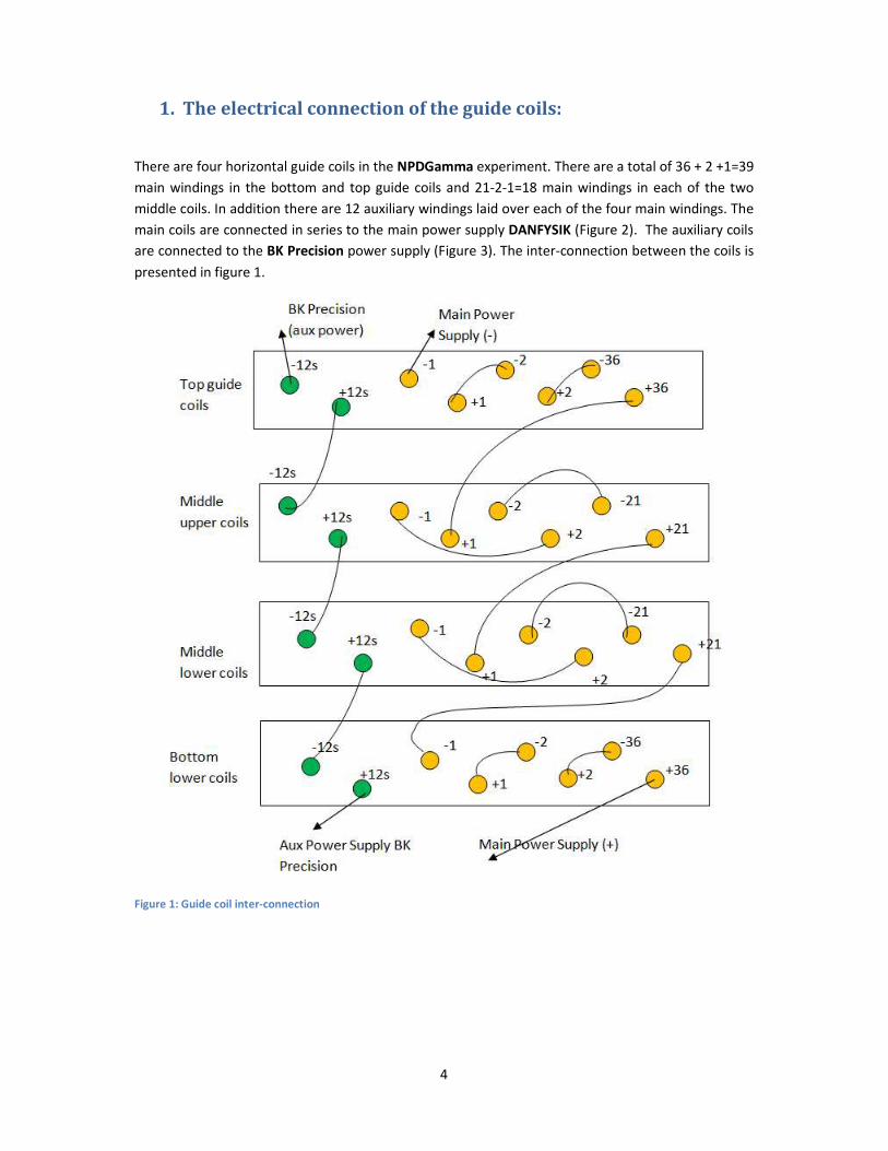
1. The electrical connection of the guide coils:

There are four horizontal guide coils in the NPDGamma experiment. There are a total of 36 + 2 +1=39

main windings in the bottom and top guide coils and 21-2-1=18 main windings in each of the two

middle coils. In addition there are 12 auxiliary windings laid over each of the four main windings. The

main coils are connected in series to the main power supply DANFYSIK (Figure 2). The auxiliary coils

are connected to the BK Precision power supply (Figure 3). The inter-connection between the coils is

presented in figure 1.

Figure 1: Guide coil inter-connection

5

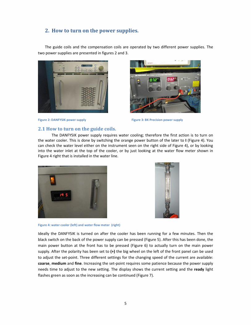
2. How to turn on the power supplies.

The guide coils and the compensation coils are operated by two different power supplies. The

two power supplies are presented in figures 2 and 3.

Figure 2: DANFYSIK power supply Figure 3: BK Precision power supply

2.1 How to turn on the guide coils.

The DANFYSIK power supply requires water cooling; therefore the first action is to turn on

the water cooler. This is done by switching the orange power button of the later to I (Figure 4). You

can check the water level either on the instrument seen on the right side of Figure 4), or by looking

into the water inlet at the top of the cooler, or by just looking at the water flow meter shown in

Figure 4 right that is installed in the water line.

Figure 4: water cooler (left) and water flow meter (right)

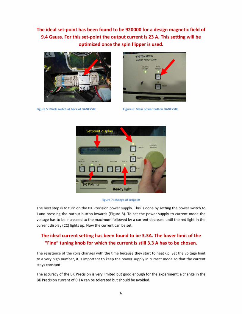
Ideally the DANFYSIK is turned on after the cooler has been running for a few minutes. Then the

black switch on the back of the power supply can be pressed (Figure 5). After this has been done, the

main power button at the front has to be pressed (Figure 6) to actually turn on the main power

supply. After the polarity has been set to (+) the big wheel on the left of the front panel can be used

to adjust the set-point. Three different settings for the changing speed of the current are available:

coarse, medium and fine. Increasing the set-point requires some patience because the power supply

needs time to adjust to the new setting. The display shows the current setting and the ready light

flashes green as soon as the increasing can be continued (Figure 7).

6

The ideal set-point has been found to be 920000 for a design magnetic field of

9.4 Gauss. For this set-point the output current is 23 A. This setting will be

optimized once the spin flipper is used.

Figure 5: Black switch at back of DANFYSIK Figure 6: Main power button DANFYSIK

Figure 7: change of setpoint

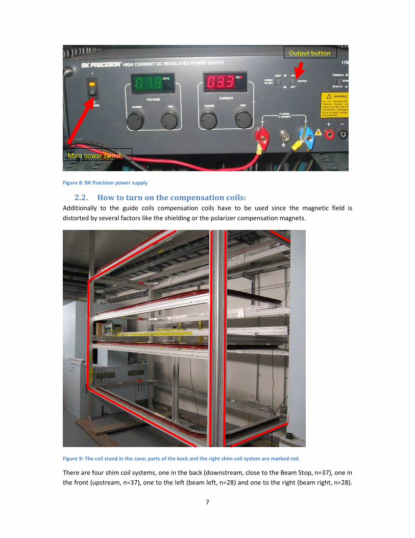
The next step is to turn on the BK Precision power supply. This is done by setting the power switch to

I and pressing the output button inwards (Figure 8). To set the power supply to current mode the

voltage has to be increased to the maximum followed by a current decrease until the red light in the

current display (CC) lights up. Now the current can be set.

The ideal current setting has been found to be 3.3A. The lower limit of the

“Fine” tuning knob for which the current is still 3.3 A has to be chosen.

The resistance of the coils changes with the time because they start to heat up. Set the voltage limit

to a very high number, it is important to keep the power supply in current mode so that the current

stays constant.

The accuracy of the BK Precision is very limited but good enough for the experiment; a change in the

BK Precision current of 0.1A can be tolerated but should be avoided.

Ready light

Setpoint display

(+) Polarity

7

Figure 8: BK Precision power supply

2.2. How to turn on the compensation coils:

Additionally to the guide coils compensation coils have to be used since the magnetic field is

distorted by several factors like the shielding or the polarizer compensation magnets.

Figure 9: The coil stand in the cave; parts of the back and the right shim coil system are marked red.

There are four shim coil systems, one in the back (downstream, close to the Beam Stop, n=37), one in

the front (upstream, n=37), one to the left (beam left, n=28) and one to the right (beam right, n=28).

Output button

Main power switch

8

They are located on the outer side of the coil stand. Figure 9 is trying to give an idea of the shim coil

positions.

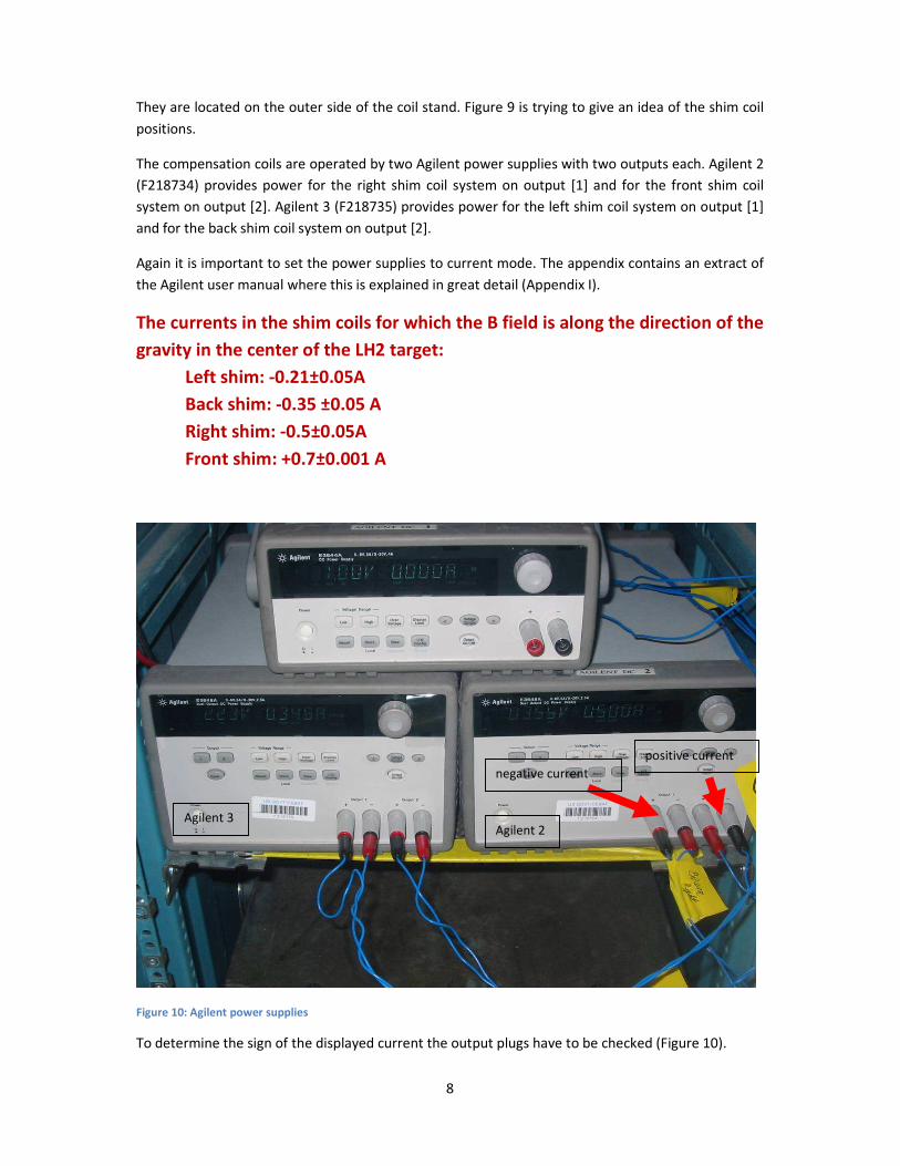
The compensation coils are operated by two Agilent power supplies with two outputs each. Agilent 2

(F218734) provides power for the right shim coil system on output [1] and for the front shim coil

system on output [2]. Agilent 3 (F218735) provides power for the left shim coil system on output [1]

and for the back shim coil system on output [2].

Again it is important to set the power supplies to current mode. The appendix contains an extract of

the Agilent user manual where this is explained in great detail (Appendix I).

The currents in the shim coils for which the B field is along the direction of the

gravity in the center of the LH2 target:

Left shim: -0.21±0.05A

Back shim: -0.35 ±0.05 A

Right shim: -0.5±0.05A

Front shim: +0.7±0.001 A

Figure 10: Agilent power supplies

To determine the sign of the displayed current the output plugs have to be checked (Figure 10).

negative current

positive current

Agilent 2 Agilent 3

9

Red connected to +: positive current

Red connected to -: negative current

3. Remote control of Power suuplies The Danfysik power supply and the Agilents can also be controlled through the PC. There are

separate reports on the wiki how this can be done. The control programs (THe VI’s) are on the

COMPAQ-PC that also performs the magnetic field readout. The BK precision power suppply cannot

be remotely controlled.

To enable power supply settings, or to readout the magnetic field, the user has to login first. Usually,

the “labuser” account should be used (with the password fpiAy2__ - note the two unserscore-signs at

the end). The administrator account is called myadmin and has the password npdgRoot__, but as

usually, shouldn’t be used unless necessary.

On the desktop, the user finds the folder NPDG_Remote. It contains the files”

- ag2.vi: This labview program controls the Agilent power supplies. See the separate report.

- df2.vi: This labview program controls the Danfysik power supply. See the separate report.

- fg2new.vi: This labview program reads the fluxgates. See next chapter.

4. Measuring the magnetic field with the flux gate sensors: First the DAQ Module has to be turned on: this is done by moving the little lever to On (Figure 11).

Figure 11: DAQ Module for flux gate sensors

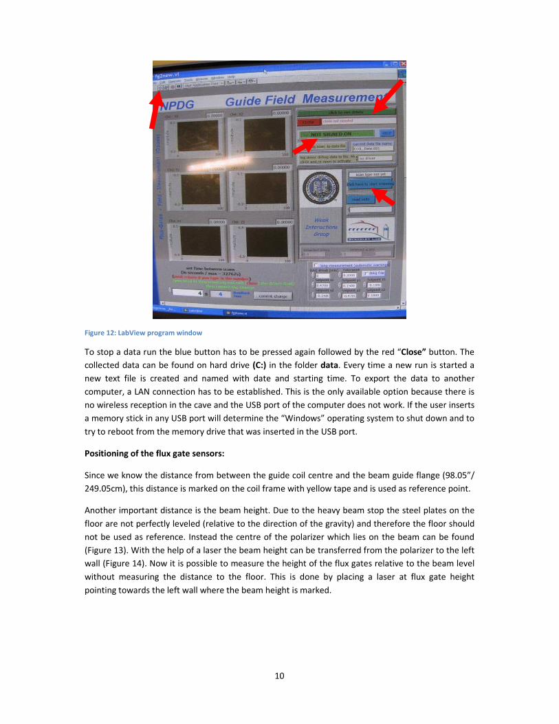
To display the measurements the LabView program has to be started on the computer. The user has

to open the folder NPDG_Remote located on the desktop and then click the LabView program

fg2new.vi. After the program has been opened the LabView run button (white arrow) has to be

pressed, followed by the green button that says click to run driver. After a few seconds the sign

“NOT SIGNED ON” will change to “SIGNED ON” and the blue button click here to start scanning has

to be clicked to start the data acquisition (Figure 12). LabView displays the data for two flux gate

sensors. Flux gate 557 is sensor one and flux gate 654 is sensor two, this order should not be

changed.

10

Figure 12: LabView program window

To stop a data run the blue button has to be pressed again followed by the red “Close” button. The

collected data can be found on hard drive (C:) in the folder data. Every time a new run is started a

new text file is created and named with date and starting time. To export the data to another

computer, a LAN connection has to be established. This is the only available option because there is

no wireless reception in the cave and the USB port of the computer does not work. If the user inserts

a memory stick in any USB port will determine the “Windows” operating system to shut down and to

try to reboot from the memory drive that was inserted in the USB port.

Positioning of the flux gate sensors:

Since we know the distance from between the guide coil centre and the beam guide flange (98.05”/

249.05cm), this distance is marked on the coil frame with yellow tape and is used as reference point.

Another important distance is the beam height. Due to the heavy beam stop the steel plates on the

floor are not perfectly leveled (relative to the direction of the gravity) and therefore the floor should

not be used as reference. Instead the centre of the polarizer which lies on the beam can be found

(Figure 13). With the help of a laser the beam height can be transferred from the polarizer to the left

wall (Figure 14). Now it is possible to measure the height of the flux gates relative to the beam level

without measuring the distance to the floor. This is done by placing a laser at flux gate height

pointing towards the left wall where the beam height is marked.

11

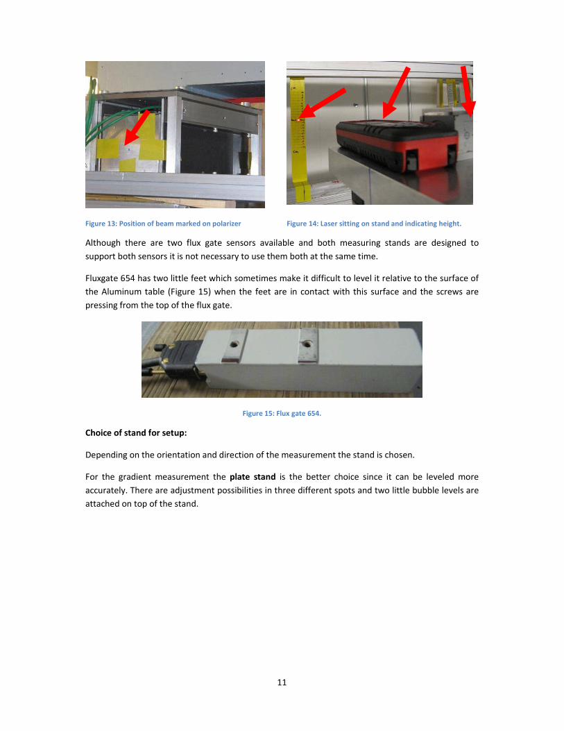
Figure 13: Position of beam marked on polarizer Figure 14: Laser sitting on stand and indicating height.

Although there are two flux gate sensors available and both measuring stands are designed to

support both sensors it is not necessary to use them both at the same time.

Fluxgate 654 has two little feet which sometimes make it difficult to level it relative to the surface of

the Aluminum table (Figure 15) when the feet are in contact with this surface and the screws are

pressing from the top of the flux gate.

Figure 15: Flux gate 654.

Choice of stand for setup:

Depending on the orientation and direction of the measurement the stand is chosen.

For the gradient measurement the plate stand is the better choice since it can be leveled more

accurately. There are adjustment possibilities in three different spots and two little bubble levels are

attached on top of the stand.

12

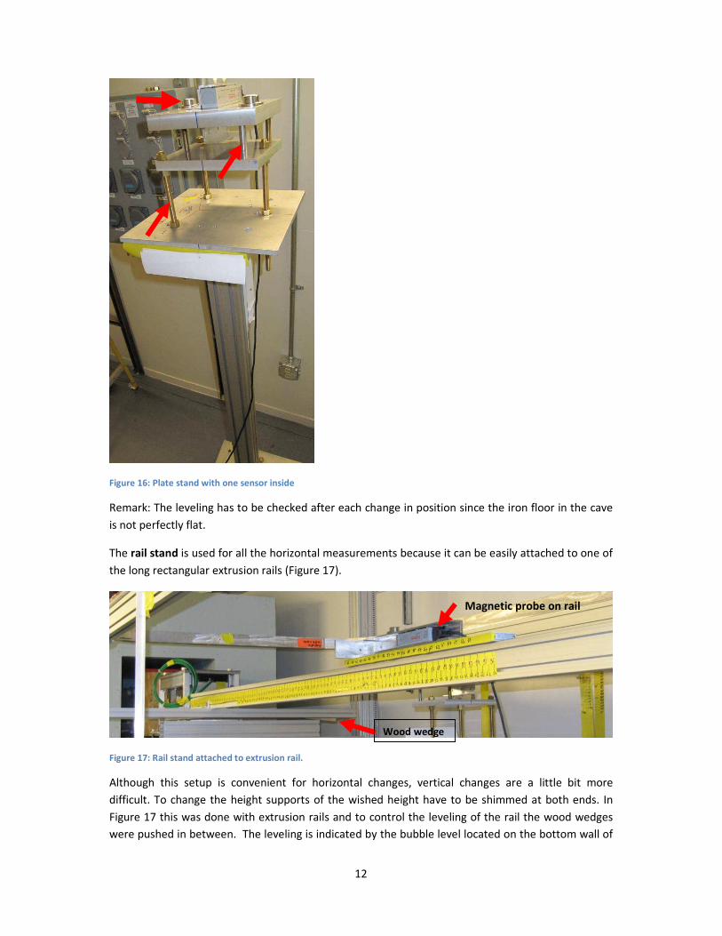
Figure 16: Plate stand with one sensor inside

Remark: The leveling has to be checked after each change in position since the iron floor in the cave

is not perfectly flat.

The rail stand is used for all the horizontal measurements because it can be easily attached to one of

the long rectangular extrusion rails (Figure 17).

Figure 17: Rail stand attached to extrusion rail.

Although this setup is convenient for horizontal changes, vertical changes are a little bit more

difficult. To change the height supports of the wished height have to be shimmed at both ends. In

Figure 17 this was done with extrusion rails and to control the leveling of the rail the wood wedges

were pushed in between. The leveling is indicated by the bubble level located on the bottom wall of

Wood wedge

Magnetic probe on rail

stand

13

the Aluminum case with two compartments where both the two sensors can be fixed simultaneously

with plastic screws.

5. Accuracy of measurements.

All the distance measurements are done with the Leica DISTO D330i distance laser (Appendix II), a

caliper or a measuring tape.

Laser accuracy: ±1mm

Measuring tape accuracy: ±1/6 "/±1.6mm

Caliper accuracy: ±1mm

The leveling is done with bubble levels.

Leveling accuracy: ±0.02°/ 0.00035rad

Appendix III contains calibration certificates for both flux gates:

Flux gate sensors accuracy:

The misalignment of the three sensors for the Flux gate 654 (MAG2) are

X 1: 0.0022 radians

Y 1: 0.0034 radians

Z 1: 0.003 radians

The misalignement for the three sensors inside the Fluxgate 557 (MAG1):

X 2: 0.00096 radians

Y 2: 0.0023 radians

Z 2: 0.00025 radians

The offset of the sensors are the fields read by the three sensors when the probe is placed in zero

magnetic field. The offset fields are given in the calibration certificate for both fluxgates :

Fluxgate 557 : X1=+3.5 nT, Y1=-10.5 nT, Z1=-3.5 nT

Fluxgate 654 : X2=-6.5 nT, Y2=0, Z2=-10.5 nT

2

3