Embed Size (px)
Citation preview

Technical RePort Number 138May 1994
AN APPROACH TOGROUNDWATER MONITORING WELL NETWORK DESIGNRELYING ON NUMERICAL TECHNIQUESAND PUBLIC.DOMAIN INFORMATION
By
John J. Quinn,Howard D. Mooers,Hans-Olaf Pfannkuch
minnesota water resources research center

AN APPROACH TOGROUNDWATBR MONITORING WELL NETWORK DBSIGN
RELYING ON NUMERICAL TECHNIQUESAND PUBLIC-DOMAIN INFORMATION
John J. Quinnr'3, Howard D. Mooers2, Hans-Olaf Pfannkuchl
Technical Report Number 138
Water Resources Research CenterUniversity of Minnesota
St. Paul. Minnesota
Mav 1994
'Department of Geology and Geophysics, University of Minnesota, Minneapolis2Deparlment of Geology, University of Minnesota, Duluth3Present address: Argonne National Laboratory, Argonne, Illinois
This constitutes the final report for a WRRC project directed by Hans-Olaf Pfannkuchand Howard D. Mooers of the Deparbnent of Geology and Geophysics, University ofMinnesota entitled: Groundwater mapping and the determination of the optimum levelof information for the assessment of groundwater sensitivity to contamination incomplex glacial-drift aquifers. This project was funded for the period July 1989 toJune 1991.
The work upon which this publication is based was supported by a grant from theUniversify of Minnesota Water Resources Research Center through the WaterResources Research Institutes Program of the U.S. Geological Survey, as authorizedbythe Water Resources Research and DeveloDment Act of 1984.
Contents of this publication do not necessarily reflect the views and policies of theU.S. Deparrment of the Interior, nor does mention of trade nzunes of commercialproducts constitute their endorsement by the U.S. Government.
The University of Minnesota is an equal opportunity employer and educator.
Water Resources Research CenterPatrick L. Brezonik, Director
1518 Cleveland Avenue, NorthUniversity of Minnesota
St. Paul, MN 55108(612) 624-9282
Fax (612) 625-1263

Table of Contents
INTRODUCTIONObjective and approachThe Anoka Regional Sanitary Landfill.Monitoring GuidelinesDesign of monitoring well networksLeachate and tracer plumes in sandy surficial aquifers
METHODSGlacial geology mapping proceduresHydrogeological glacial facies modelingGroundwater modelinsGeostatistics
STUDY AREARegional setting: glacial geology of east-central MinnesotaLocal study area
MODELING GROUNDWATER FLOW AND LEACHATEMIGRATION
Hydrogeological facies modelKriging the basal elevation of the aquiferFlow modelingAdvective transport modelingAnalysis of results
SUMMARY
REFERENCES
III4
4
5
1l11
l3
77
7
8
202020253235
39
41

ABSTRACT
Uncertainties in the hydrogeology of a study area and in the transport properties of potential
contaminants challenge the aesigners of groundwater monitoring well networks- Numerical flow
modeling is a useful iool for guiding the placement of wells, but it requires justified boundary
conditions and sufficient knowledge of aquifer parameters. In a graciated terrain, additional
problems arise because of complex spatial arrangements of aquifers and aquitards. The transport
of conservation contaminant tracers is normally calculated as a simple function of average values
of hydraulic conductivity, hydraulic gradient, and effective porosity. But are the results of this
straightforward method always valid?
In order to address these topics, this investigation focused on a landfill on the Anoka sandplain of
east-central Minnesota. The purpose of this study was to determine the proper placement of an
initial group of monitoring *"ttr at the landfill using only offsite public-domain data. The results
may then be applied to the siting of other wells.
Finite-difference flow modeling was supported by an abundance of inexpensive public-domain
information and by the construction of a detailed, sub-regional glacial geologic map. A two-
dimensional kriging analysis refined the model by determining the cell-by-cell best estimates of
the basal elevation of the surficial aquifer. Particle tracking results indicated the expected
pathway of landfill leachate. Based on the results, one well upgradient of the landfill and several
iowngiadient wells were selected from the database of actual monitoring wells, and the head data
from these shallow wells were used to calibrate the model. The calibrated hydraulic conductivity
of the sandplain aquifer agrees closely with values obtained through grain-size analyses and pump
tests. Numerical analyses of boundary conditions support the validity of the flow model'
Other case studies of unconfined outwash aquifers suggest that predicted plumes of conservative
tracers are often greater than the actual extents. Compared to the chloride data for monitoring
wells at the Anoka site, particle tracking results have an accurate orientation but a length at least
two times too long. Uncertainties, such as the effect of longitudinal dispersion and the transient
nature of the leachate's initial concentration and source area, suggest an even greater difference'
This conceptual understanding of plume migration provides guidance for the placement of
additional downgradient wells. The described application of models and inexpensive offsite data
to monitoring well network design is a methodology that may be effective for the monitoring of
solutes from existing or proposed potential contamination sources.
ACKNOWLEDGEMENTS
This project benefitted from the geostatistical expertise of Dr. Randal J. Barnes of the Department
of Civil and Mineral Engineering. Several individuals supplies data that were useful in this
project. They include Perry Jones, U. S. Bureau of Mines; Jane Cleland and Emily Bauer,
ir,linn.rotu Geological Survey; Kerry Keen, Twin City Testing; Matt Landon, IJ- S. Geological
Survey, Shelly Burman and Wayne Sarappo, Minnesota Pollution Control Agency; and Bob
potocnik, Minnesota Department of Natural Resources, Division of Waters- Thanks to Bob
Tipping, Peter Jansson, and Gail Lowry Haglund for their computer assistance, and to the
Limnological Research Center of the University of Minnesota for access to their excellent
Macintosh computer facilities. Dr. Herbert E. Wright of the LRC provided guidance on the
glacial geology portion of this project

INTRODUCTION
Obiective and aPProachA groundwaler contamination investigation involves 1 large. financial expenditure, much of
which is spent in tdiltaitution or -onii":fiil;;itt. ny,rrstiddressing a site using available
data and techniques, monitoring wetts^mit e pg;irtonfo ut locations that optimize sampling
"bpfi;r, ""-ify tttl ait"Ction fra extent of poteirtiat contaminant migration'
rhe purpor;-of ,hir-;6dy it ;;'i;il16;;;rh;d rol d:,_"1=1T,':g, th" placement of
monitoring wells at an existing-o, por.n-ti"l-ro*d" of groundwater contamination. The approach
makes use of offsite public-domuin iniot*ation iri a hvdrogeologic investigation utilizing
groundwat* orooriil/"#;;;,'ff,.ical techniques to adoteri the migration of conservarive,
advectively t -rportfr conti-inar,tr. -A.,
e*t"nsi''e monitoring well nitwork at a landfill near
Anoka, Minnesota serves only as an unui"iJ-eans of calibrati'ng the.flow model and checking
the dependability oi tr," i"ro[s. The """ii"[ili v "f ".tr"t onsite data is conducive to a practical
case study with an approach -relying on-;]it-*ql ly&g.g"otoet-:,^111ysis rather than a
hwothetical scenario. This study may serve as a means of guidlng mbnitoring well placement at
;ili";;ir"t, especially those in similar geologic settings'
The Anoka Regional Sanitary LandfillThe Anoka ;i;;# S*ilu"y r-#drtu (Anoka landfill) is loc-ated.in the citv of Ramsev in
sourhwestern Anoka county, Minnesota (Figure 1), approximately 20 miles (32 km) to the north
of Minneapolis. Housing develop."nL'.J nonri'rici west of tlie landfill (Figure 2)' Another
,oUai"irioi, Hunteri HiUi is one-'half mile (800m)-to the.southeast'
The tandfil history is described;;;;ril ui Hictgt and Foth & Van lrE (1987)' .Inlate1967 the ciry of Ar;i:ilJs;;;;-ildniii"s "p".itionr
in an abandoned sand'and eravel pit- The
65 acre (T7 hectare) waste disposar *"r'#;?;f#;;;;;ilt" iou""tion svsrem. fhe elevation of
the base of the wasre is approximut"f'liO fT (ZOS m). At the time oi the 1993 closure' the
maximum elevarion including tte cap'witii"'r,-oz+ i'(ltz.t m) (s. Kollodge, 1989, personal
"o-rnoniintion), which is abo-ut 150 ff (45 m) abowe 8nde.
The predo#i,iiti *"rp-ryp; dip;sea or in de Anoka landfill is mixed municipal wastes
with smaller amounts of foundry t-dt, fi;tn, -*d
a"-oiition waste' During-the y:ars prec-:gig
its rgT1State Sohd iv;6F"#rit, toweu'et, tlre A-ng\a landfilr also received hazardous wastes m
the form of paint sludges and paint thlnneis. In addition, the landfill accepted llqtl *g^g:ilt1,h; ;iil
"iAnom waltewatei treaunent plant during this period.' No liquid waste' matenals ln
drums, or materials currently classifii'a;il;ddr"." b"ti"ued to have been disposed of at the
landfill since the lg72 permit; only municipal and other non-tt-.oous wastes have been accepted'
In recent y;;;-;A,h o] auru truTb";;;gi"pit.l on site conditions at the Anoka landfill,
including *el fogs]*JLr*t*"tion aJuifs, aquifei Pump tests,. and temporal analyses of heads
and water quality i-urrr.t"rr. e gro.rni-*utei nionitoring network was begun in 1972 to evaluate
the potential fot gto*fuui"icontimination. As of 1987 the database included:' .77-onitorilf;;ii;ar;"gb*""iioi"gwettt,ocationsand Z}locat\onsof ness of 2to
5 wells),'23 Piezometers,'6 soil borings, and
'i aquiferpu-mp-test-wells , r: --- ^cr'.^ .-.aa+a rio-ncor qrpq Tn 'l ego thearranged around ,h;;;i",;irt-rtt" majority downgradient of the waste disposal area' In 1990 the
network had grown to include t*o *or" iquif"t"trrt wells and ten more associated piezometers
(Foth & Van Oyrc, f 9S%), ang t*o uaaitioiuf bedrock wells @oth & Van Dyke' 1990)'
Approximately quarterly r*.rphd giwells began in the 1970s, providing a large database
of spatial anO.temporat ctanges.in he"ads and waler quality paratieters, including general
parameters, -u1or-io'*, t "uuy
.ietals, and volatile organic compounds'

Nlinnesota
Sherburne Co.
Is.trr ts'i.gs
Wright Co.
miles
0510t-Altl
0 510
Figrge I - Location of landfill. The square represents the border of the 300 rni2 (780 l<rn2)
glacial geology mapping area of Quinn (1992).
Anoka Co.
ltLandAnok
o
Hennepin Co.
Minneapolis o
Ramsey Co.
St. Paul

A.f.\5-t q tE-t\.w
vw - 6Ata 6rll\\'6 ;gn.. n^ 5Ccoo.ud
,.-..n iVfW 4'--::3-". j zsz.zs
alsEl
uy-a,ta
aw-:
rAIt
rzro
r=r,E I:
titi
lt
))--1(il.lr*
;ilr,llil"tl
\h*II 'll I//\,/\l
PT.5o
0 mile A.25
-
o km 0.5:
\ s3lclt\ril ^tz-tft v
//,/ .tt't<<,/-
Icr-:t lrrl
ztr 533zt38
als!E!
to,. P:-6
-4:.-
w.lAF
5r rt
ev-2!3a
s9I
Ilw- 293!.l
sa llo
/ u*-n" n'/ \.\
/ ' ''e'1 '|// A, \lt
/ rv-'',lP r.szc..,l/
,[ \ i'
l::;z iEa /",,!'\ \,
f .L,"v:,;ff' /,,i / \\\y?,,
Monitoring guidelinesFedaral-guidelines dealing with groundwater monitoring are generally ambiguous and open
to a great deal of interpretation. IiT ttre case of a waste disposal site, the monitoring schemeis to be
comfrised of four monitoring wells: one located upgradient from the site and three in the directionof groundwarer flow (NW.WA and U.S. EPA, 1986; Aller and others, 1989). These arereqlirements for an initial network only; once contamination is detected -the
gl-oundwatermonitoring effort is augmented to delineata the horizontal and vertical extents oJg^e pJITg and.todetenninJthe rate of iontaminant migration (Aller and others, 1989; U.S. EPA, 1986). Thegrowth of the network is norrnally done in a step-wise fashion, so that information obtained fromJample locations may guide the placement of future sampling. The guidelines, however, cannotsupfty specific information dealing with, for example, the proximity of wells to a possible sour. ce
of p-oituion or the depth at which the wells shouldbe screened. ^9{ ptig-y concem is_assessing
the impact to the uppermost aquifer (NWIilA & U.S. EPA, 1986). But i1 a case of complexhydrog^eology, path*ays to deepEr aquifers may exist, and they may _be difficult to determine.
tnaiviairat states may ihoose to adoprregulations more stringent than those of the U.S.EPA (Aller and others, 1989). Normally the monitoring well network design nege9qqry to definethe hydrogeology of a site is ultimately determined by a regulatory ag9!c_y_Qgg:ht, 1990).-
ffr'e Mi-nnesota Rules (State-of Minnesota, t989, chapter 7035.2815) provide generalrequirements for the monitoring of mixed municipal solid waste disposal facilities. Theseguidelines allow a subjective appioach to designing a groundwater monitoring network. The rulesItate the basic purpose of moniloring wells: the early detection of the pollutants from a faciliry andthe determination bf the spatial extent of pollutant concentrations. In order to comply, the. number,placement, types and depths of monitoring points around a site must be chosen ac-cording to an
ivaluation oiitre hydrogeologic setting, which includes an assessment of potential contaminantpathways. Additiohal monitoring points need to be constructed in the event of the detection ofcontaminants.
Because of the inherent variability of geologic deposits, interpretations of these guidelines-
may vary widely among investigators and result in different monitoring schemes. Case studies ofmohitor6d sites may piovide tfie best resource for future network designs at other facilities insimilar hydrogeologic environments.
Design of monitoring well networks- Ai area of growing emphasis in the literature focuses on the various approaches ofmonitoring well networks. Specifically, many researchers are striving to develop a method for theoptimization of well placement. Studies of this sort arc often theoretical in nature.^
Meyer and Biill (1988) proposed a computationally intensive technique for monitoring wgllnetwork d6sign that relies on an optimization model to choose locations that maximize theprobability ofplume detection. Loaiciga (1939) developed a methd of optimization based onmass tranlport-modeling, statistical accuracy, and economic constraints. Massmann and Freeze(I987a,1987b) included groundwater monitoring aspects in an elaborate risk-cost-benefit analy.sis
of potential pollution sources. Freeze and others(1990) and Massmann and othen.(199t) Ptoyde^a thorough introduction to the importance of geology and engineering in decision -analysis ofhydrogeological studies using a risk-cost-benefit function. This approach may be applied to wellnetwork design.
Pfannkuch (1975) addressed the problem of determining the optimal amount of informationneeded for assessing hydrogeologic uncertainty. He proposed that the worth of additional datacould only be quaniifi-ed if the benefits of the extra effort could be economlgal]y calculated.Pfannkuch and Labno (1976) detailed a step-wise approach to optimum well placement thatstresses the various objectives and constraints associated with the design strategy.
Other efforts to determine optimal monitoring well placement involve some form of spatialanalysis such as laigrng. Spruill and Candela (1990) demonstrated the use of loigilg to gain.amaximum of knowl&ge aom a minimum of monitoring wells in a regional water quality netygrfc.They compared the data needs for this objective with the greater amount of information needed inthe
-case of determining a mean or median parameter concentration value for the region.

Mcl-aughlin and Graham (1986), in a_cokriging.analysis,.showed how the spatial correlation and
"ross-c6oelation of hydraulic'conductiviiy,-head, and chemical concentration may aid in
monitoring well network design.
Leachate and tracer plumes in surficial sandy aqurfelsSeveral ,"""nt rtidi"t investigat6 the characieristics of contaminant plumes in unconfined
glaciofl uvial aquifers.e fimmet and Braids (1980, 1974) examined the impact of two landfills in Long Island,
New york. Extensive monitoring well networks allowed them to observe the three-dimensional
rutor"oittrr plumes. They fouid a downward component of leachate movement beneath the
l*anlfi, utrifuted to a aeniity contrast between contaminated and back^ground waters. Slugs oftfr" tittt-;r;sity leachate are b6[eved to flow downward through the aquifg after recharge events-
" Chloride is a common component of landfill leachate. Because chloride is-generally-non-
reactive, it serves as conservative ^tracer of contaminant movement (Davis and others, 1985). A
conservative tracer would be expected to travel at the same rate as the average linear gtoundwater
velocity, according to Darcy's law: K.iv =; Fq'1
where v = average linear groundwater velocity [LT-l],K = hydraulic conductivity [LT-l],i = hydraulic gradient [unitless], andne = effective porosity [unitless].
A key finding of Kimmel and Braids (1980) is that a gr.eat difference between the expected
chloridi plime locition based on the darcian approximation and the actual plume location
supporred by the field data. The theoretical extent of the plumes, equal to v multip{*-Uy F.. ,i-9tiriJ" l""ati[ing ueEun, is 3 to 4 times longer than the actual-extent. Even if leaching ofcontaminants dif, not"occur until sometime aft& the opening of the landfills, this disagreement is
difFcult to rationalize.MacFarlane and others (1983), using an elaborate, high-density monitoring.well network,
studied a landfill located on a glaciofluvial iquifer in Ontario. Their frndings were similar to those
of Kimmel and Braids (1980)"in that the leachate plume has a downward component benea,h,h:land{ill and then traveli -ore hoti"ontally at depth in the aquifer. They attribute the downward
movement to up to three possible factors: iiownwardhead gradients produced by a transient water-
table mound b6neath the^landfilt, greater density of leachate, and lower viscosity of leachate as a
result of heat generated by miciobial activity in the plume. At this site, a wide range ofconductivities iere estimat6d using grain-size analyses, permeameter tests, slug tests'. and pump
r"16.- Uri"g the geomerric mean fiidrautic conductivity obtained with each methd P.Sug*pred.icted cdnserv-atirre contaminant plumes of 0.5 to 1.5 times the extent of the actual chloride
;ffi;. Thtactuat plume, howevei, exhibited pronounced-longitudinal dispersion,.with low;hfiAr .-on."nt*tio'ns throughout the downgradi^ent half 9f th9 plume. The theoretical extent ofth;-pfttitt.i"fot" *as muih less than th-e extent predicted us-ing most of the conducti-vity
deteimination methods. The authors suggest two reasons for the disagreement of theoretical vs-
il;;f pffi" length: small-scale heterogle-neities in the aquifer, and errors in the various methods
used to determine hydraulic conductivity values.Robertson *d oth"tr (1!91) pehormed bromide traces in two sandy surFrcial aquifers and
in one case found the groundwater velocity indicated by the tracer to be half of the velocity
"uf"ufat"a using permeaineter-estimated hydiaulic conductivity and average effective porosity- In
.ontruit to th" iuitanU studies, this tracer experiment is free of uncertainties related to the source,
such as the transient nature of contaminant reiease and the changing areal extent of landfilled waste.
In some cases the theoretical plume may match the actual plume. Mackay and others
(19g6) i"tr*"a chloride and bromide tacers, as-well as several organic solutes, into an outwash
;q"if*. They actually found the conservative tracers to travel faster than the average linear

groundwater flow velocity predicted using conductivity values obtained through slug tests, grainsize analyses, and and perrneameter methods. They attribute the discrepancy to errors in theestimates of hydraulic conductivity, hydraulic gradieng and effective porosity.
Dispersion is a factor which could affect the distribution of conservative tracers. However,plumes in unconfined sand aquifers have been shown to have negligible transverse dispersion(Robertson and others, 799L; Kimmel and Braids, 1980, L974; Mackay and others, 1986).MacFarlane and others (1983) attribute lateral spreading of the landfrll's plume to slight seasonalchanges in groundwater flow directions. Vertical dispersion was found to be negligible in all ofthe above studies. Because of the infiltration of recharge, clean gloundwater is typically above avertically narrow plume downgradient from a contamination source. The effect of longitudinaldispersion, however, may be very difficult to evaluate, especially in studies that do not involve acontrolled tracer experiment
6

METHODS
Glacial geology mapping proceduresDetaitedreconnaissance-level glacial geologrc mapping can be accomplished by a synthesis
of information compiled from airphotos, topographic maps, and soil surveys.Low-altitude (1:20,000-icale) black-and-white air photos from the University of
Minnesota's Borchert Map Library are a valuable mapping tool. Stereo-pairs are available from a
wide range of years. In suburban areas, older series that were -photogtapld plor-lo extensivedevelopment are most useful in discerning various glaciogenic features. Tunnel val]eys, 9qkep,kettles, dunefields, and paleo-drainageways are distinguished effectively by working with thestereepain in addition to topographic maps.-Soil
surveys indicate the distribution of various soil types, from whigh the glacial parentmaterials may be inferred. The surveys serve as a cross-check of air-photo interpretations in thecase of delindating the zones of alluvial soils or mucks found in former meltwater draina_geways orin peaty kettles. They are especially useful in distinguishing the borders of outwash or till units.- -Glaciogenic
ilems of interest were delineated on 1:24,000-scale topographic gg{rqglep.This informatibn was then transcribed onto a mylar overlay of a portion of a 1:100,000-scaleUSGS planimetric map.
Hydrogeological glacial facies modeling- A facies model serves as a framework for interpreting and predicting the geology of a given
sedimentary environment (Walker, 1984). Glacial geologic facies models are useful in determi_ninglarge-scaletrends and distributions of different glaciogenic-units Gyleq and Miall, 1984; white'I91q. A glacial facies model is a generalized assemblage of sediments that are representative of acertain glaciological depositional environment (Eyles, 1 98 3)-
Recent -studies have emphasized the hydrogeological importance of such models
(Anderson, 1989, 1987a, 1987b;-Fraser and Bleuer,1987; Stephenson and othgrs,, 1988). Byunderstanding the surficial and buried sedimentological units in tenns oftheir glacial genesis, o-ne
develops ttre aUitity to predict the distribution of aquifers an{ aqgltards. These studies are_usuallyconcerned with large-scale facies because of the difficulties in evaluating small-scaleheterogeneities (Anderson, 1989).-Glacial process models have been proposed for terrains associated with portions ofMinnesota (Mooers, 1990, 1988; Chernicoff, 1983, 1980). Models such as these may form the
basis for initial hydrogeological facies models useful in assessments of particular areas.
Groundwater modelingFinite difference ntodcling and MODFI'OW
A finite difference groundwater model is a numerical approximation of a flow syqtem.Conceptually, this technique is simple. The area of interest is chosen and discretized by.a-finitedifference grid. Boundary conditions are assigned to the model according to available or inferredhydrologiCfeatures. The choice of the type of boundary conditions and their locations maynecessitate a change in the configuration of the modeled area. Flow equations are assigned.to each
cell in the model depending on aquifer type and stresses imposed on the system., Thg eOgglions are
solved by an iterative method. Discussions of equations and applications are found in Wang andAnderson (1982) and Anderson and Woessner (1992), respectively.
For a cell in a steady-state, t'wo-dimensional model of a homogeneous, unconfined aquifer,flow is calculated by the Boussinesq equation:
*(".'*) . *(""H) = -R 4.2

where h = sarurated thickness (head - base of aquifer) plX,Y = Cartesian coordinates [L],
K*,y = hydraulic conductivity flT-ll, andR = recharge [LT-t].
In the finite difference method, these derivatives are replaced by differences, and thesolution is found by iterating to a specified convergence criterion. The-calculation of a cell'stransmissivity_inco_rporates the varying saturated thickness of an unconfrned aquifer.
MODFLOW is a versatile finite difference model written by McD<inald and Harbaugh(1988). The model handles a multitude of hydrogeologic and anthropogenic factors. MODFLOIVwas chosen for use in this study because it is well documented, well tested, and its output can beutilized in a particle tracking program. In addition, a finite difference model was desired^because itcan easily incorporate an input array of geostatistically determined values.
. - -^\t9ry.lVdrogeologic literature contains numerous examples of frnite difference modeling,and MODFLOW is the code used in many of these papers.
Advective transport particle tracking and MODPATHMODPATH (Pollock, 1989, 1988) is a semianalytical particle-tracking program for
determining steady-state groundwater flow paths in block-centered hnite d.ifference-rnodeTs. One-,two-, or three-dimensional anaiyses may be performed.
Flow velocities are determined by the flow model, MODFLOW, for each face of each finitedifference block. The particle-tracking method assumes that the velocity in each coordinatedirection varies linearly between the velocities calculated at each face by the flow model. From thisinformation, MODPATH derives an analytical expression for the flow velocity distribution of eachcell. In a two-dimensional model, the path of any particle can be computed from the two-dimensional velocityfield. The flow paths are calculaied exactly by MODPAitt based on the finitedifference flow m69el9ytpur. The^flow model, however, ii a'simplification of a system, andtherefore the MODPATH results are only as accurate as the MODFLOW output. In-a parricle-tracking model, dispersion is ignot{, and_flow is by advecrive rransport only. Particlei may betracked forward (for example, to estimate flow paths from a contaminint sour6e) or backward-(forexample, to determine recharge areas).
GeostatisticsGeostatistics involves the application of speciai statistical tools to spatially correlated data.
The..basic premise of geostatistics is that samples that are close togettrer -witt
g6nerally be more$-ilq in so-me parameter of interest than samples that are far aparr. This spatiat Iorrelation may beinvestigated in geostatistical studies of one, two, or three dimensions.^ Isaaks and Srivasiava(1989), Knudsen (1988), and deMarsily (1986) offer introductions ro the subiect.
Variograns
- The experimental variogram quantifies the spatial structure of a data set and is determinedbv
YG) = *; [Z(xi+h)-Z(x)]z F4. 3
where {h) = variogram value for separation distance h,
tr = separation distance between points (lag)"Nn = number of pairs of separation distance h,
Z(xi) = value of sample at location x, andZ(x1+h) = value of sample at location x+h.
Although the symbol y{h) is actually the semi-variogram, this study will use rhe commonconvention of simply referring to it as the variogram.
N1
i=1
The variogram equation calculates the average squared difference for pairs of data. Thegraph of y(h) vs. h, using the data, is called the experimental variogram. Modeling involveschoosing a variogram type (for example spherical, linear, exponential, etc.) and determining theparameters that produce the best fit of the experimental variognm. These parameters usuallyinclude the nugget effect (Clo), the range (a), and the sill (C). The nugget effect is the 1(h) valuewhen h=0; it quantifies extremely short-range variability. Data are correlated up to a separationdistance known as the range. Past the range, the data are uncorrelated and the variogram value isthe ultimate sill, which is equal to the sill plus the nugget effect.
Typically, the maximum h allowed in a variogram calculation is equal to roughly one-thirdto one-half of the maximum extent of the data. Beyond this point the variogram may break downas a result of too few data pairs. Summaries of typical model variograms and their conespondingequations ire presented in deMarsily (1986, p. 301-303), Knudsen (1988, p.42-46), and Isaaksand Srivastava (1989, p.372-375).
A data set may exhibit anisonopy with respect to its range; that is, the range may bedifferent in different directions. Anisotropy is often not visually apparent in a data set and can beobserved only in directional variograms. The variogram results can therefore discover andquantify geologic factors which are otherwise not visible. In a rwo-dimensional study, followingthe construction of a satisfactory omnidirectional variograrn, a directional variogram analysis maybe performed by specifying a search direction and an angular tolerance. For example, fourdirectional variogram search directions may be oriented E-W, NE-SW, N-S, and NW-SE, eachwith an angular tolerance of at least 22.5o.
Ordinary KigingKrigrng is a geostatistical tool for optimal interpolation of spatially correlated data. It is
often described as a minimum-variance, linear, unbiased estimator. By weighting nearby samplesaccording to the krigtng algorithm when estimating the value of a parameter of a point or a block,the variance of the estimate is minimized. Ordinary loigt.tg is the type of kriging most commonlyperformed in geological applications because it does not assume a particular value for the localmean; estimation therefore takes into account only the local samples.
The following equation relates the estimated value of a block with neighboring data:n
Z* (r) = I Ii Z(xi)i=1
estimated value of block v,number of nearby samples,value of sample at xi, and
w.4where z" (u)
nz(xi)l.i = Lrigng weight of sample i.
The kriging weights, 1.1, are found by the use of the Lagrange parameter. The krigingweights are used in the calculation of the kriging variance of each block, which represents thevariance on the error of the estimation. This error is modeled bv a normal distribution.
VARIO and Geo-EASVARIO is a varioglf{_ pogr-am deye]oped by Dr. R.J. Barnes of the University of
Minnesota Deparnnent of Civil and Mineral Engineering. Experimental variograms may beproduced fiom one-, two-, or three-dimensional data, and anisotropy analyses may be performed.Most variogram programs use a lag increment to group classes of data when plottine theMost variogam programs use a lag increment to group classes of data when pexperimental variogram. VARIO, however, utilizes a smoothi.ng parameter, which has units ofleng4, The smoothing effect is produced by calculating a moving average of points within aspecified window. Because the smoothing algorithm gives the user a large degree of conrrol{*ing refinement of the variogram, it produces more representative variograms than the lagincrement method.
gme

Geo.EAS (Geostatistical Environmental Assessment Sofrware) is a geostatistical computerpackage developed for the U.S. EPA and documented by Englund and Sparks (1988). Geo-EAShandles experimental and model variograms, kriging, and several support functions. Data setsmust be two-dimensional. Krigrng options include choices between ordinary and simple krigrng,and block and point krigrng. Point krigrng is the estimation of the value of a point based on thekrigrng of nearby samples. Block laiging involves the use of an array of points (2 by 2, forexample) for each block in a grid, then kriging with these array values to determine the estimate ofeach block. Point and block kriging usually yield similar estimates; however, point krigrngproduces higher lrigrng standard deviations.
10

STUDY AREA
Regional setting: glacial geology of east-central MinnesotaIntroduaion
The surficial geology and landfomrs of east-cennal Minnesota are primarily the result oftwo Late Wisconsin ice advances: the Superior lobe and the Grantsburg sublobe (Wright,I972b). Earlier Pleistocene advances had previously deposited drift throughout the region.Despite interglacial erosion and the reworking and redepositing of older deposits by the morerecent ice lobes, some older drift presumably underlies the Late Wisconsin deposits throughoutmuch of this region. However, due to a lack of deep exposures and only generalized sub-surfacedescriotions in well loes. characterization of the historv. thickness. areal extent, and texture ofdescriptions in well logs, characterization of the history, thickness,the older deposits is difficult.
extent, and texture ofdescriptions in well
Superior lobeThe Superior lobe emanated from the Lake Superior basin and advanced to a position
southwest of the Twin Cities area (Figure 3a) during its Late Wisconsin maximum, the St. Croixphase. The resulting St. Croix moraine generally has a breadth of about 6 miles (10 km) incennal Minnesota (lilright, I972a). The southwestern portion of the moraine has a northwest-southeast-trending segment bordered on much of its northeastern, inner side by the MississippiRiver valley. Radiocarbon dating of lake sediments indicates that the Superior lobe reached itsmaximum extent prior to 20,500 + 400 years before present (Wright and others, 1973), althoughClayton and Moran (L982) suggest a somewhat younger date.
The Superior-lobe deposits reflect the bedrock geology along the lobe's path and aretypically red in color. The till is normally sandy in texture. Characteristic litho-logies fromnortheast Minnesota present in the drift include red sandstone, basalt, amygdaloidal basalt, andred felsite (Wright and others, 1973).
Tunnel valleys and esken commonly occur together in the area glaciated by the Superiorlobe. The tunnel valleys may have been eroded by geothermally or frictionally generatedsubglacial meltwater (Wright, 1973) or by supraglacial meltwater penetrating to the base of theice via crevasses (Mooers, 1988, 1989). Eskers are often present within the tunnel valleys andwere presumably deposited by waning meltwater flow. The eskers represent the position of thesubglacial stream as the deforming ice constricted the flow. Eskers are much narrower thantunnel valleys, and two or more sub-parallel eskers may be present within a tunnel valley.
The tunnel valleys are normally straight or slightly curved and trend to the southwest.This direction is oblique to the regional slope, but it parallels the inferred ice gradient andtherefore is in the direction of decreasing hydrostatic head flilright,1973).
The tunnel valleys range in width from <590 ft (180 m) to >3,300 ft (1,000 m), with anaverage of about 980 ft (300 m) (Wright" 1973), and they are about 33 ft (10 m) deep In lengththey vary geatly (Wright, 1973), although most segments are 6 to 12 mi (10 to 20 km) long(Mooers, 1989). The eskers are normally discontinuous features within or along the sides of thetunnel valleys, and their crests are usually equal in elevation to the adjoining till plain (Wright,1973). Fairly continuous segments are generally less than about 2.5 mi (4 km) in length(Mooers, 1989).
Grarxsburg sublobe and Arnka sandplainThe Des Moines lobe advanced from the Red River Valley of northwestern Minnesota
down the Minnesota River Valley to the valley's bend at Mankato. From this point the ice flowednortheasterly into the Minneapolis Lowland as the Grantsburg sublobe (Figure 3b). Afterthickening sufficiently, the sublobe overtopped the Sr Croix moraine along a length of 75 miles(120 km) from Minneapolis northwest to Albany (Wright and others, 1973). The glacier flowedin a northeasterly direction as far as Grantsburg, Wisconsin, over the area recently vacated by theSuperior lobe. The Grantsburg sublobe reached its maximum position about 16,000 years ago(Wright and others, 1973) during its Pine City phase. Ice of the Des Moines lobe propereventually thickened enough to pass a topographic barrier and flow south into Iowa, reaching its
11

B.A.
Figure 3 - I-ate Wisconsin glaciations affecting east-cental Minnesota. A. Superior lobe and the
St. Croix Moraine. B. Grantsburg sublobe (modified from Wright, 1972b).
Figure 4 - Development of the Anoka sandplain. A. Maximum extent of Grantsburg sublobe.
B. FIow around the wasting lobe as the sandpiain evolves. Keewatin tiil is Grantsburg sublobe
tiil, and "E" is Cooper's "Elk River Morainic Area" (from Cooper, 1935).
L2

maximum extent at Des Moines 14,000 years ago (Wright and others, 1973; Clayton and Moran,1982). Because the main lobe chose this new path, the flow of ice to the Grantsburg sublobediminished. The sublobe stagnated, and the ice margin wasted back to the southwest as theglacial Mississippi River continuously shifted its course (Figure 4), distributing ounvash over an
area of 850 mi2 (2,200 tm2) Garnham, 1956). This outwash plain, together with the adjacent,slightly younger deposits of the Mississippi valley train, is known as the Anoka sandplain-
Unoxidized deposits of the Grantsburg sublobe are typically gray and calcareous. The tillis generally silry and contains fragments of Cretaceous shale and lignite from western Minnesotaand clasts of Paleozoic carbonate mainly from Manitoba (Wright and others, 1973). In theoxidized zone, however, the drift is light brown in color.
Tunnel valleys and eskers are not known to be associated with the Grantsburg sublobe(Chernicoff, 1980, 1983).
Numerous kettle lakes and other depressions abound in areas glaciated by the Superiorand Grantsburg advances. The melting of buried pieces of ice produced these topographic lows,which may today be occupied by peatlands, swamps, or lakes. Stagnant Superior-lobe ice waspresent within the kettles and tunnel valleys during the advance of the Grantsburg sublobe. Thisdead ice preserved the morphology of these depressions during the deposition of Grantsburg tilland/or the Anoka sandplain. Even the eskers within the tunnel valleys are easily discernable(Wright, 197 2a, I97 2b).
Local study areaT\e23 frz 69 6o2; tocal study area, for numerical modeling and geostatistical analysis,
is bounded on the southwest by the Mississippi River, on the east by the Rum River, and on thenorth by Trott Brook @gure 5). The western boundary is an inferred no-flow boundary whichis discussed in the modeling section of this study.
Hydrogeology of surficial san"dsThe advances of the Grantsburg sublobe and the Superior lobe, in addition to pre-Late
Wisconsin glaciers, have produced a complex assemblage of deposits of widely varyinghydraulic conductivities. However, the surface of the entire local study area is covered withsands of the Mississippi valley train and the Anoka sandplain.
A detailed study by Quinn (1992) of an area covered by six 7.5-minute U.S. GeologicalSurvey topographic quadrangles (Anoka, Nowthen, Elk -River, Rogers, Coon Rapids, and
Cedar) producea u *up of the surficial geology of a 300 rni2 (780 km2) region centered aroundthe Anoka landfill (Figure 1). The purpose of the mapping exercise was to closely examine thearea's glacial geology in order to better understand the sedimentary associations closer to thelandfill. Figure 6 shows a portion of this map representing approximately 100 , z Q60 km2).The Anoka sandplain aquifer, comprised of Mississippi valley train sands and the Anokasandplain proper, covers the entire modeling area.
Several shallow sandpits are located about I mile (1.6 km) south of the Anoka landfill(Quinn, 1992). These sandpits are the only known geologic exposures near the landfill. Thesediments range from poorly sorted coarse sands and fine gravels to moderately sorted mediumsand. Samples from texturally different crossbeds of the exposed Mississippi valley-train sandsprovide a means of estimating the hydraulic conductivity of the medium by two empiricaltechniques: the Hazen method (Floltz and Kovacs, 1981) and the Krumbein and Monk (1943)method. Porosities of the samples were also determined in the laboratory. Data and graphs areprovided by Quinn (1992). A comparison of ttre hydraulic conductivity results shows quite closeagreement between the values determined by the two methods. The conductivities obtainedthrough these methods range between approximately 3.9x10-a to 2.4x10⁻³ f/s (I.2x70-2 to7.3xlt.2 cm/s). Although these values do not provide an exact representation of the sandplain'srange of permeability, they do support an average initial value of -1.2x10⁻³ ftls (-3.5xt0-z cmls)for the modeling of the surFrcial sandy aquifer. This K value is typical for outwash sands (e.9.
L3

ll;arll s8ll =ill €
=lt =(!ll cs -V
II E €ll I all+.1ild3II E File'Ell : EIle
il} 5ll dsll E bII } E AII E 8 Ell .hff- -a C)
ll gEEil-€!ll'h'=ll ,., E 5ilqefll ;o.* ?ll t E I
:il
z
\!
zol
)Y
I
14

\a'-:'l>J::lttryj
Zfl$::::;i:::::rir:5i:p iiiii:ii*iirrUiiiii:ii as ii:i :?i
../1. -. -... -..... -tt^' .. .
r' \-7-- i::::::l:::r\ i\...,......\
iiiit
N
;iij":."rfiffiri'
kilometers
-
012345milesr0r23
Undifferentiated Lowlands. Topographically low areas presently occupied by peatbogs, wetlands, lakes, and floodplains of creeks and rivers. Includes former tumelvalleys.
Mississippi Valley Traln. Sands deposited by the glacial Mississippi River. Thevalley traia is distinguished from the Anoka sandplain and from recent floodplairs byelevation differences and by large braided channel pattens visible on air photos.
|!FT] Anoka Sandplain. Outwash sands and gravels disributed by the glacial Mississippi|:: as : ] River as the Gransbwg sublobe wasted back to the southwest.F. '{
Grantsburg Sublobe Ground Moraine. Gray ro buff frne-grained till.
Eskers. Sand and gravel deposited in the Superior lobe's sub-glacial runnel vaileys,which are characterized by iong, southwest-trending topographic depressions thatrypically contain eskers.
t:l St. Croix Moralne. A opographic high indicating the maximum extent of the Superiort- sc -i lobe. The moraine is blanketed with Crantsburg till in this study area.tt
\ y lakes. rivers. creeks. ma-ior ditches
---'W the Anoka Regional Sanitary Landfill (near center of map)
Figure 6 - Surhcial geology surrounding the Anoka landfill (modified from Quinn, 1992).
fJ
15

Freezn and Cherry , lg7g, p. 2g), and is within the range of 7x10-a to 2x10⁻³ fils (2xI0-2 to
7xl0-2 cm/s) estimated by Helgesen and Lindholm (1977) for the Anoka sandplain. It should be
noted that ttrese empiricai K va]ues are for particular samples of surficial Mississrppi-valley-trainsands. They do nof necessarily represent the average conductiviry of sal-ds of the valleytrain-orthe Anoka iandplain proper
-etsdwhere in the study area, either areally or stratigraphically.
However, reasonably ilos6 agreement is expected. This K value simply provides p appropriatefirst approximation ior the nyArautic conductivity of the surficial sands; it is subject to change
during the calibrration of the numerical model." A slight anisotropic component of permeabiliry may be imparted to fllvial sand duringdeposition.
-Sand graini deposited by a uni-directional current exhibit imbrication; that is,
eldngate grains are lignen paiallel to the crurent direction and thgV dip upstream at an angle.of J0to 25" fr5m the horiz-ontal-(Potter and Mast, 1963). This imbrication produces a fabric in theporous medium which is aligned with cross-bed dip directign. The orientation of the direction ofina*imom permeability has6een shown to be aligned parallel to cross-bed direction in sandstone(Mast and Potter, 1963) and in unconsolidated Holocene sands (Pryor, 1972).
In the local study area, large braided channels are visible on air-photos. Although theflow of the Mississippi v-alley train-was generally to the southeast, the surfrcial ch-annels are quiteserpentine, without^an apparent overalftrend. Strike and dip measurements taken at the threesmitt sandpits near the lindfill indicate widely varying crbss-bed orientations. Silrce onlysurficial information is available, general trends-in the saturated zone axe not known. Based on
this information, the slight small-scale directional permeability imparted by depositionalprocesses is considered nEg[gible, and the surficial sand aquifer of this study is assumed to be
isonopic.
Hydrogeology of deeper drift"Of tne l,SZ logs of phvate wells inspected in the local study area, all describe a thickness
of surficial sand and fmvei (mean thiclness 47 ft or 14 m). Most then encounter a unit describedas "gray clay" by thJdritters. The remainder of th_e logs show q l'..luy'.--ol"brown c-lay" be-lgw
the ian'clplai-n. This is interpreted to indicate that Granisburg sublobe till forms the base of the
surficialiandplain throughout the modeling area. This buried till unit is the same as the exposedGrantsburg sublobe ground moraine of the northern portion of Figure 6.
Hydraulic conductivity analyses of Gransburg till yield a K11of 2.5xlt6 to 3.0x10⁻⁷ fVs
(7.7x10-i to 9.Ox10-6 cm/s) oUtuin"O by slug/baildown tests and a Ky of 1.5x10⁻⁸ to 7.5x10⁻¹¹
frls (4.5x10⁻⁷ to2.3xl0-9 cm/s) from laboratory tests (K. Keen, 1991, wrinen communication).' Studies of fine-grained tills in North America have demonstrated that a surficial till is
expecred to have an uppEr, weathered zone that is hydrologic?llyacti_ve,-belonlvhich the till is an
univeathered, unfractGed aquitard (e.g. Ruland and others 1991; Hendry, L9F2,1988; Cravensand Ruedisili, 1987). However, Williams and Farvolden (1967) and Ruland and others note aminor amount of fracturing into the deeper, unweathered zone. No examples were found in the
literature which address the possibility bf fractures in deep, buried tills. No studies concernedwith characterization of fractures in Minnesota tills are known.
Within the modeling area, the buried Grantsburg sublobe till appears to be continuous and
of appreciable thickness. Therefore this unit is assumed to be an aquitard in the study area-
Below the Grantsburg sublobe till the drift is believed to be a complex assemblage-ofSuperior lobe till and outwaih, and pre-Late Wisconsin drift. This arrangement is generallysupported in the study area by inspection of drillers' logs.
The three-dimensional correlation structure of the glacial drift units in the study area has
been investigated using geostatistical techniques by Quinn (1992) and Quinn and others (1992).
16

Bedrock geology and hydrogeologyAttrictisequenie of sedimentary rocks of Cambrian and OrQgyician-.ages exists above a
faulted Precambrian basement in southeastern Minnesota (Austin,1972). Within the study area"
the bedrock is predominantly the Cambrian St. l-awrence and Franconia Formations (Austin,1972;Jnsaandbthers, 1986; Olsen and Bloomgren, 1989).
The St. Lawrence is comprised of silty, sandy, shaley, and dolomitic rocks (Austin,t972). Its expected thickness is approximately 50 ft (15 m), howevel4e upper surface of theformation is partially eroded in the vicinity of the landfill (Austin, 1972). In the Twin Citiesbasin the Frariconia Formation is typically a fine-grained glauconitic sandstone and siltstone, witha thickness of about 155 ft (47 m) (Mossler, 1972). A few isolated knobs of Jordan Sandstonehave been mapped, and buried bedrock valleys are cut into the Ironton-Galesville and the EauClaire Formations in the region (Jirsa and others, 1986).
The St. LawrenceFormation is considered to be a confining unit (flogberg, 1972;Kanivetsky, 1989). The underlying Franconia Formation has apermeable upper portion, but ispredomindntly an aquitard ftIogberg, 1972; Walton, 1986). The 51, I awrence and FranconiaFormations hi've been modeled as a iingte confining unit in a Twin Cities regional aquifer studyby Schoenberg (1990).-
Below ttre Franconia are the Ironton and Galesville Sandstones, which are productiveaquifers (Hogberg, 1972). The Franconia, despite th_e low.p,ermea.bilityof its lower half, issometimes cdnsid-ered part of the Franconia-Ironton-Galesville aquifer. An inspection of thepotentiometric head of ihe Hennepin County portigq of this system su_ggests that it discharges to^the
Mississippi River (Kanivetskn 1989), presumably through the St. LawrencelFranconia (Jirsa
and others, 1986; Kanivetsky, 1989).
Surface warcrsBecause of the high infiltration rate of the sandy soils of the Anoka sandplain, the area
near the Anoka landfrll has few strearns or ditches.The Rum River flows to the south about 2 miles (3 km) east of the landfill (Figure 5). A
USGS gagrng station is located on the Rum about 5 miles (8 km)_upltrqam froP the confluenceof the Rum River and Trott Brook. Discharge information from U.S. Geological Survey walelresources data indicate that river stages at thii station generally fluctuate between 862.7 ft (263.0
m) to 866.3 tt(264.0 m). On the 7.5-minute topographic maps, the contours that cross the Rumnear this station correspond closely to the expected value of the river stage. The contourscrossing the Rum Rivei along the eastern border of the study area are therefore assumed torepresent the average river stage at each location.^
The Missisiippi Riveiflows southeasterly less than 2 miles (3.2 km) south of the AnokaLandfill. A USGS gugtng station is located 6.5 miles (10.5 km) down_streary from Anoka, near
Coon Rapids. HowEver, the station is on the downstream sfdg o{ qhe Cogn Rapids dam, which,according to the topographic map, causes a drop of about 19 ft (5.8 m). Upstream from Anoka,the nexi gaging staiion is at Elk River, but data collection there ceased decades_qgo.Consequeitly, no accurate temporal values are available for the stage of the Mississippi Rivernear the landfill.
Trott Brook is a perennial stream located 3 miles (5 km) north of the landfill within a
runnel valley (Figure 6)-. No gaging station exists along the brook to aid in validatilg.thgcontours crolsingit on the topograptric maps. The topographic contours crossing the MississippiRiver and Trott Brook are assumed to represent average river stage conditions.
Within the local study area, all three drainageways are located on the Mississippi valle-y
train and/or the Anoka sandilain. Because of the permeable nanlre of their setting, they ar-e {]expected to be in direct contact with the shallow groundwatgr floy s.yslem: *Lindgren (1990)dehonstrated the strong hydraulic connection between the Mississippi River stage andobservation wells in the valley train aquifer. Ericson and others (1974), in a regional hydrologystudy, mapped the Mississippi, the Rum, and Trott Brook as gaining streams.-
Wh-ether Trott Brobk is truly a gaining stream on both its northern and southern issomewhat questionable. It is even more uncertain as to whether the brook serves as a discharge
t7

point for the entire saturated thickness of the Anoka sandplain aquifer. Ditches and streams areknown to provide partial to complete capture of groundwater in unconfined flow systems(Chambers and Bahr, L992:Zheng and othen, 1988b). No field data are available to characterizevertical or horizontal hydraulic gradients in the vicinity of the brook. Zheng and others (1988a)developed an equation relating the depth ofcapture ofditches to several hydrogeological factors.This approach, however, calls for the ditch or stream to be located on a linearly sloping watertable. Because the brook is believed to receive discharge from both banks, the method of Zhengand others is not applicable. In this study, Trott Brook, like the Mississippi and Rum Rivers, isassumed to function as a constant head boundary. That is, these waterways are assumed toreceive discharge from the entire saturated thickness of the sandplain on both banks.
Lakes are common in the pitted sandplain and valley train. Because they are located inhighly perrneable basins, these lakes are also expected to be in direct connection with the surficialsand aquifer. The Minnesota Department of Natural Resources Dvision of Waters compiles dataon lake levels of four Anoka County lakes situated on the sandplain near the city of Anoka.These include Crooked, Round, SunRstr (Grass), and Itasca (Figure 5). At Sunfish Lake,however, the monitoring program has been in effect only since 1989. The lake levels (Figure 7)reflect seasonal and year-to-year changes in the stresses on the shallow groundwater system,including recovery after the drought years of 1988 and 1989. Although only infrequent samplingoccurred at Sunfish Lake after 199I, the data indicate an anomalous dip in lake level that isprobably due to remediation at the landfill. Because the shallow groundwater is expected tointeract closely with these sandplain lakes, general changes in the water table should closelymatch the lake level changes. The close similarities of lake level changes among the four lakessuggest that pre-1989 levels of Sunfish Lake may be approximately extrapolated to aid inestimating the water table elevation near the landfill for the period of 1985-1989.
875
860
1 984 1 986 1 988 1 990 1 992 1 994
Figure 7 - Lake level changes of fbur lakes situated on the Anoka sandplain, withrn or nearthe local study area (data from Minnesota Deparrnent of Natural Resources).
870
oo
; 865goJg
18

Recharge to tle Arnka SandPlainitt tfte bcal study area the mean annual precipitation is about 28 inches (71 cm), iq"lfqing
the contribution from sriowfall, which averages 45 inches (114 cm) annually (Kuehnast, 1978).
Expected characteristics of the permeable soils developed_on a sandplain include highinfiltratiori, high evapoffanspiration, and low surface runoff. Precipitation and snowmelt,therefore, prim-arily either recharge the groundwater 9r arg lost to e-vapotranspiration. Helgesen
and Lindholm (1977) performed a two-year study of the hydrographs of 8 water tableobservation wells on the Anoka sandptain. They catculated an estimated average annual recharge
to the surficial aquifer of 11 in (28 cm).
Lacal Flow SystemAn inipection of the average stages of the Missi-ssippi and Rum- Rivers and the Trott
Brook, togeth6r with lake level data, indicate that groundwater near the landfill is. expected toflow in a ioutheasterly direction. However, the configuration of streamlines in the vicinity-of the
landfill remains unknown because the landfitl should be on or near a gtoundwater flow divide.The orientation of the streamlines will be addressed in this study by a combination of numericalflow modeling and advective transport modeling.
Becau"se of the possibiliry bf increasediecharge in the waste disposal area, a water table
mound may be present bneath i landfrll. Slight mounding has^b^een shown to occur at unlinedtananUs (lvtacfartane and others, 1983; Kehew and Passeio, 1990), although MacFarlane and
others demonstrated that the mound was a transient feature that occurred in conjunction withsnowmelt and spring rains. The possibility of mounding is-unliSgly at the Anoka landfill because
of high infiltration capacities of both the sandplain anq the landfill.In Ramsey township, homeowners reiy on private_wells for their drinking water supply.
Aninspectionofthelogsofwellsintheloca|studyareaindicatedthatnearlyallofthesewellsarefinished in either the fermeable portion of the Franconia Formation or in the deeper IrontonFormation.

MODELING GROUNDWATER FLOW AND LEACHATE MIGRATION
Hydrogeological facies modelThe private well log data support a fairly simple hydrogeological glacial facies model for
the local rygy.ar9a.- Tle uppermost unit of this model-is comprised oT the Anoka sandplainlquifer, which.includes the Anoka sandplain and associated Mississippi valley-train sands.^ Thethickness of this unit is approximately 47 feet (14 m). The sandplain is unconfomrably underlainby Grantsl'urg-sublobe tilJ, as ilqe_lpreted from the drillers'descriptions and suppofied by glacialgeological studie.s-(Chernicoff, 1983, 1980; Wright and others, 1913). This till ir^nit is exfected tobe continuous with the-ground moraine in the north-central portion of Figure 6. The Grantsburgtill is alsuTed to provlde a suitable aquitard, thereby reducing the modeling effort to include onl!the surficial sand aquifer.
This model may seem simple, however, a facies model may not include all locallldrogeologtpal features (Fraser and Bleuer, 1987). Even a relatively simple geologic frameworkdoes not preclude the possibility of surprising stratigraphic arrangements.
Kriging the basal elevation of the surficial aquiftrThe transmissivity of_a_surficial aquifer is dependent on two variables: the hydraulic
conductivity and the saturated thickness, which is a function of the elevations of both the watertable and the base g{ tt q aquifer._ An investigation of the flow system of an unconfrned aquifermust therefore consider the spatially varying basal elevation of the aquifer.
This phase of the study involves a geostatistical analysis of the areal distribution of theelevation of the contact between the Anoka sandplain aquifer and the underlying Grantsburgsublobe.till a.guitard. The.study area is represented by cells with dimensions of 660 ft by 660 it(201. m Ay ?9t m). This is the same grid as that in the finite difference groundwater modelingportion of this study.
The database^f91 this analysis is the drillers' logs of 152 private wells (Figure 8). Astatewide inventory of this information is maintained at the MinnesoraGeological SurvJy @GS).
Several sources of error are inherent to the data set. First is the estimation of th-e elevationof the land at the wellhead. Addresses supplied on each well log facilitated the locating of eachproperty on a county plat map-..An approximate topographic value for the top elevation ofeach logwas then determined by checking the corresponding location on a USGS 7.5-minute topographilTap. This may-result in.an error of up to-5 feet (1.5-m) for the elevarion of the top of *16 w?lt tog.Consequently, the elevation of the sand/till contact would be off bv the same amounr.
. .4 problem affecting the quality of the data is that they were not recorded for use in as,cientific analysis; rather, logging was a perfunctory task. For several reasons, the recordeddep$s- to geologic contacts_.mal be regarded with some degree of suspicion. The logging wascqry4 out by numerous individuals from different contracrois. MGS pbrsonnel wtro aiJfairiUarwith the methods of local drillers describe that when drilling through drift, the stratigraphy islogq$ primarily- Uy th9 spe$ at which the drilling is progressing: fast implies sand or gro:nei sio*implies a till or lacustrine clay. Seldom are samples-takEn or observations made of ti'e maierialswhich are lpughl up.in drilling fluids- Some logs contain fairly detailed stratigraphy while others9n^ly describe units that are greater than 50 feet (15 m) thick, suggesring th-at some amounr ofinformation is often unrecorded. AIso, the depth to contacts may be affectJO Uy boreholes that arenot vertical or straight.
Variogrwn results
. The variogram investigation was carried out using the program VARIO. Directionalvariograms were calculated with an angular tolerance of 22.5o (Flgure 9). This two-dimensionalexamination_produced a linear model variogram with a nugger of 240 tt2 (ZZ m2; and fairly stronganiso_nopy Figq:lOa). lhe experimental omnidirectionafuariogram is iinear ihrough a dista.tcEof 25,000 ft (7,600 m), after which th.e variogram breaks down due to a lack of Eata at largeseparation distances. An additional directional variogram, oriented north-northwest to sout[-
20

\I
{Ro\-sR9
o"1'0 mile 1:
0bnl
Figure 8 - I-ocations of wells used in geostatistical
anaiyses.
i,l
a 82'r. well location andelevation of base ofsandplain aquifer
Figure 9 - Exampie of a two-dimensional
represents an east-west search for a given
directional variogram search area The shaded area
data location, with a tolerance angle of 22.50.
-
21

360
3-10
320
300
280
260
210
22020,000
A.
10,000
Distance in feet
WEST
B. sourH
Fisure 10 - A. Omnidirectional and directional linear variograms for the basal elevation of the
,"ioot*. B. Anisotropy ellipse for the variograms of the basai elevation of the sandplain- Plotted
values are the ftmges corresponding to an arbitrarily chosen y(h) vaiue of 350 ft2'
North west-S outh east
North-South
East-West
Northeast-S outhwest --.Omnidirectional
NORTH
SOUTH
22

southeast, has the lowest slope and therefore represents the direction of maximum range.Geostatistical anisotropy is often illustrated by an ellipse, with major and minor axescorresponding to the axes of geometric anisotropy. In this investigation the anisotropy is orientednortlr-northwest to south-southeast with a ratio of approximately 3:2 (Figure 10b).
Because the nugget effect is equal to the variance of the data at zero separation, the nugget
of 24A fl Q2 m2; indicares a standard deviation of 15.5 ft (4.7 m) at h=0. This value may beattributed to geotogic complexity, lack of careful logging, the error related to estimating theelevation of the land at the well location, or a combination of these factors. However, the relativeimpact of each cannot be determined.
theIn order to detemrine the sensitivity of the directional variogram to the angular tolerance,)rance was oDened up to 30o, allowing the comparison of more sample pairs. Thetolerance was opened up to 30o, comparison of more sample pairs. The
; when compared to the analyses wirh22.5"variograms, however, showed no noticeable differences when compared to thetolerance angles.
Two possible geologic interpretations of the observed anisotropy are offered. The glacialMississippi river, during the formation of both the Anoka sandplain and the Mississippi valleytrain, had a generally southeastern flow direction in this viciniry (Figure 4). Erosion by meltwaterstrearns trending in this direction would have produced the spatial correlation illustrated by Figure10. Another possibility is the influence of glacial depositional processes associated with the flowdirections of ice lobes. As discussed previously, in the study area the Superior lobe flowedsouthwesterly, and the Grantsburg sublobe advanced northeasterly @igure 3). These flowdirections are both essentially perpendicular to the northwest-to-southeast trending anisotropy.The Superior lobe's St. Croix moraine, located along the southwest border of the study area, hasthe same trend as the spatial structure. This topographic influence on the depositional processesassociated with these two most recent advances could have imparted some of the spatial corelationstructure apparent in the variogram analysis.
KrigingOrdinary laiging incorporates the anisotropic structure revealed by the variogram analyses
to produce the best estimate of the sandplain's basal elevation at each grid cell in the study area. To
determine the slope of a linear variogram, Geo-EAS requires specification of a YG) and theconesponding h value (Table 1). The kriging estimations for the sand/till contact are contoured inFigure 11. The cell-by-cell values of this output are utilized as input in the MODFLOW numericalmodel of groundwater flow in the study area.
Linearvariogram modelNuggetEffect = 240 fP (22 m2>
Major Rangel = 17,000 ft (5,200 m)Minor Rangel = 11,000 ft (3,600 m)
SiI Vatuel = 350 t& 1lZ mzlAngle2 = 112.5" (NNW-SSE)
Maximum Points3 = 16
Search Radius4 = 15,000 ft (4,600 m)
I In a linear variogram model, the range and sill simply define the slope; they are not true ftInges or sills.2 The angle is the direction (0 to 180') of the maximum range. Geo-EAS measures this anglecounterclockwise from east = 0o.3 The maximum number of data poins included in the determination of the estimate of a block.
The search radius is the maximum distance allowed in a data point search for the calculation of thevalue of a eiven block
23

"*.,-P^- .'
$6J/"f(-/ (I\,, ---z *oAScrA/-
4'(,7
4uz7
a,".L(o
\?
a'/L(f,
\?
(\\835/
.830-
935.r
2-
+"^n/- zo" *oo,"r{rr6fu
Figure 11 - Generalized contours of kriged estimates of
elevation of base of sandplain. Contour interval = 5 ft
(i.5 m).
"o.'$N
\$/l
\rce tresca
O -il-#
0km1
t^t.]Q
Figure 12 - Generalized contours of lcriging standard
deviations derived from block kriging. Contour interval
=2 ft (0.6 m).
24

Geo-EAS produced the same estimation oulput using both point and block kriging;however, the lcriging standard deviations were markedly different. For block krigrng-, the tcrigingstandard deviation was roughly 6 to 10 ft (2 to 3 m) throughout the center of the study area, withgreater values around the edges @gure 12). For point kriging, th.e value w-as about 16 to 18 ft(S.Z to 5.9 m) in the central portion. The disciepancy arises because the block-kriging.isdescribing the variance on the estimate for a large (660 by 660 ft, or 201 by 201 m) block, whilethe point kigtng variance is for comparison of individual. points (i.e. well locations). Because the^
finiie differe-ncJmodel is concerned witn me values of grid cells, the krigittg standard deviation of6 to 10 ft (2 to 3 m) represents a fairly low level of error on the estimate of cells in much of the
modeling irea- Krigin! standard deviations, however, are sensitive to variogmm parameters, and
are morJuseful for iepresenting relative error rather than accurately calculated error"
Flow modelingA deterninistic finite difference numerical model of groundwater flow in the local study
area was developed in order to quantitatively assess the flow system in the-local study area. -Theresults from the calibrated version of the flow model are then utilized by a particle-trackingprogam in order to investigate the direction and rate of migration of conservative contaminants.
The boundaries oT the local study area were chosen from inferred hydrogeologicboundaries, as described below. The area was discretized into a gnd of cells measuring 660 ft by660 ft (201 m by 207 m), using square mile sections as a base (Figure 13). With 64 cells per
square mile (about 25 cells per square km), the grid is de-signed-to represent the stud_y area at ar&sonably fine resolution.
-The effect of boundary condition discretization on heads near the
landfill is Lxpected to be minimized by the fine grid and the distance from the boundaries. The grid
N ,/ l-D Nonhwes Boundary
t(
0 mile i
0kml
Figure 13 - The finite difference gnd of the local studyarea. Specified-head boundaries are denoted by blacksquares; dots mark the constant-head boundary.Variable-head cells are white. The locations of the one-dimensional models are noted. Grid cells measure 660 ft(201 m) on each side.
1-D Tnnsient Model
25

is rectanguLar,63 cells by 53 cells. Included are I,428 variable-head cells, 163 constant-head cellsalong the three specified-head boundaries (rivers), 9 constant-head cells along an inferred constant-head boundaty, and L,739 inactive cells. The modeling is performed using MODFLOW(MacDonald and Harbaugh, 1988).
The model is a one-layer analysis. The suitability of the two-dimensional assumption willbe discussed. In this study, engineering data on heads and chloride concentrations are taken from1987, because precipitation was near normal for the year.
M odcl assurnptio rlls, initial paranwters, and boundary conditio nsFive main variables or controls affect the model: the values for hydraulic conductivity and
recharge, the effect exerted by the varying base of the sandplain, the dimensionality, and theassigned boundary conditions.- The geologic environment modeled in this study is relatively simple and homogeneous incomparison 1o many hydrogeologic settings. However, heterogeneities exist even in a sandymedium. The hydraulic conductiviry of the sand aquifer has been estimated by grain-size analyses
to be about 1.2 x 10⁻³ fVs (3.5 x 10⁻² cm/s), as discussed previously. A detailed three-dimensionaldistribution of conductivity values is not available to characterize in more detail the hydraulicconductivity of the sandplain. Therefore neither detailed three-dimensional nor stochastic modelingis possible. Instead, thls deterministic model focuses on calibrating to determine the effectivehorizontal hydraulic conductivity for the Anoka sandplain in this area of interest.
The average annual net recharge value of 11 in (28 cm) determined by Helgesen andLindholm (L977) provides a reasonable recharge value to serve as input to the model. Because therecharge parameier is substantiated, its value is held constant, and the valug for hydraulicconduCtivity is varied in order to calibrate the model. Surficial geologic mapping (Figure 6) a1d aninspection of the 152 well logs for the local study area suggest that, because of similar surficialmaterials, infiltration of precipitation may be expected to be unifonn over the entire area of interest.
Because of the contrast in hydraulic conductiviry of a minimum of four orders of magnitudebetween the sandplain and the underlying Grantsburg till, the till is considered to be an aquitard,and flow is modeled only in the surficial aquifer. Although the model consists of only one layer,including the varying base takes into account a three-dimensional aspect of the unconfined aquifer.Three-dimensional flow is ignored in the flow and particle-tracking analyses. Because this modelis simptified into two dimensions, its head oulput is a function of an effective horizontal hydrauiicconductivity for the entire sanrated thickness of sand at each finite difference cell.
Proper boundary conditions are a crucial component of a groundwater model (Franke andReilly, 7987: Franke and others, 1984). As described above, the contours on the topographicmaps of the study area are assumed to represent average stages of the Rum River, MississippiRiver, and Trott Brook. Geologic mapping (Figure 6) and an inspection of the well logs in thelocal study area suggest a highly permeable setting for the surface water bodies in the area ofinterest. The assumption is made, therefore, that the two major rivers, the brook, and the lakes inthe sandplain are representations of the shallow flow system. Constant head values for each rivercell are obtained by interpolating river stages between the locations where the contour lines crossthe rivers on the topographic maps. Heads are also specified along an unnamed perennialtributary of the Rum River near the northeast corner of the study area.
The northwest edge of the study area, however, is not modeled by a specified-headboundary. Here, Trott Brook is assumed to be a gaining stream (Ericson and others, I974), evenalong its southern bank. An inferred 875 ft (267 m) constant-head boundary is therefore set fromits position where it crosses the brook, through an area south of the brook (Figure 5).Groundwater in the northwestern portion of the study area is thereby forced to flow to both thebrook and the Mississippi River. An upgradient flux is assumed to produce this configuration ofequipotentials in this area.
The western edge of the modeling area is assumed to be a streamline, representinggroundwater flowing straight from the 875 ft (267 m) equipotential to the Mississippi. This no-flow boundarv is modeled as a linear border of active and inactive cells.

Several sources of error are inherent to the boundary condition and dimensionalityassumptions. The specified-head boundaries are not completelyjustified in this two.dimensionalmodel because the rivers are not fully penetrating. The two-dimensional modeling implies that allAnoka sandplain aquifer flow would be discharged along the stream boundaries. No informationis available to determine whether the Rum River or Trott Brook may be considered regionalboundaries relative to the entire saturated thickness of the Anoka sandplain.
Lake level data for several lakes in or near the local srudy area are available from theMinnesota Departrnent of Natural Resources. Because the lakes are considered observation pointsof the water table, the lake level data (Figure 7) may be useful as a means of calibrating the inputparameters of the flow model.
Initial resultsUsing a recharge of 11 in (28 cm) and the hydraulic conductivity suggested by the grain
size analyses of 1.2 x 10⁻³ fVs (3.5 x 10⁻² cm/s), a somewhat reasonable representation of thegroundwater flow system is determined, with groundwater near the landfrll flowing in a southeastdirection (Figure 14). However, a comparison of the water table contours with information on1987 lake levels suggests that the water table elevation is too high in the vicinity of the landfill. Anextrapolation of lake level data suggests that the level of Sunfish Lake was in the range of 858 to860 ft (261.5 to262.1 m) in 1987 (FigureT).
CalibratbnBased on the level of Sunfish Lake, the initial model run suggests that either the
conductivity value used is too low, or the recharge value is too high, or a combination of these twofactors. Because hydraulic conductivity within an outwash deposit typically ranges over severalorders of magnitude, while the annual average recharge rate varies by much less, the hydraulicconductivity is the parameter that will be adjusted to calibrate the model. The recharge value, asdetermined by Helgesen and Lindholm (1977), is held constant.
Compared to Sunfish Lake, which covers several grid cells, calibration to water levels inmonitoring wells provides greater accuracy. An initial monitoring network for any facility would
Figure 14 - lnitial results using hydraulic conductiviryderived from grain-size calculations. Contour interval =5 ft (1.5 m).
N
I
58a
10s
27

I
include one upgradient well and three downgradient wells. Based solely.on the contoured oufput,
four water tabTe -onitoring wells from afpropriate- positions were chosen from the existing
**itoring well network (Fi'gure 2). The eidvation of ihe saturated zone at each well location is
iouna in tfie engineering datiUase for a July 29, -1987
sampling €vent GgtJt ,&- V?" Py5"' 1987)'
These values -" ur"d in"calibrrating the flori model more piecis-ely than with lake level data alone.
Ti;;;gli i series of rrial-and-erroimodel runs, an effective hori2ontal hydraulic conductivity of
z.lxt64 fVs (8.2x10⁻² cm/s) was determined for the local_study area (Se.u1e 15). Th9 resulting
eouipotentials correspona *"tt to the expected summer 1987 level of Sunfish Lukg, and they march
#ffi;il;iJ;i;;i;tti iout monitoring wells adequarely, within approximatelv l. foot (0.3 m)-
Til" ;;"i r pr.ai.tJ*ut"r table elevatioi in the viciniry oi Late Itasca matches the historical data
,or""*r,"ip6orly, p"itrupi u""uuse the lake is a broad observatio-n point of the water table located
in * -r" i,r "hingili Ft""o*ater flow directions and hydrauliCgradients. Lake Itasca is also
more subject to boundarY effects-Mod.ting *;$;J;r"ted using the strongly implicit procedure (McDonald and Harbaugh,
l9gg, ctraptet tZ;. Si^xteen iterationJ were required to compute the results with a convergence
criterion of 0.1 ft (3 cm).The scale'of the model ignores local effects, such as flow near lakes or variatrons rn
hydraulic conductivity ait"iu"rlotir. e more detailed calibration of the flow model is not possible
"hrhi;,il'. ;.'"p" "rilis
stuay becayse $9 gnlv quantifred water table observation points are the
four engineering monitoring *-"ill, Sunfish Lake, and Lake Itasca.
irris griuna*ui". tioa"t ii believed to represent-the unconfined flow :-yt,:li_T.T:T9t{accurately. .d volumetric budget analysis calculated by MODFLOW indicates model rnputs ot 4-J
i,37r t6.ri m3/s) from constant-head sources (the northwest constant-head boundary) and 18.8
irrTt fo.si *ritj from recharge by precipiration. outp.ut is compris"g.of z3-2 ti/s (0.66 m3/s)to
tr,"iii.in"d-head Louno-i"i alcin! the'Mississippi fiiver, the Rum River, and Trott Brook. The
p"r"ent discrepancy of input us. o,irput is negligible at 0.467a. The oulput file of this calibrated
hodet is presented by Quinn (1992)-
The model-aet"lnin"d hydraulic conductivity value of 2.7x10⁻³ ftls (8.2x10⁻² cm/s)^agrees
well with values "dil;alhiougi
other methods. In two pump tests near the landfill, Foth & Van
zf-l LANDtil-\Jn -/
Figure 15 - The calibrated flow model. Contour interval
= 5 ft (1.5 m).
N
870

Dyke (19g9a) determined conductivity values ranglng from 1.2x10⁻³ to 4-6x10⁻³ fVs (3'6x10⁻² to
1.4x10-r crn/s) in the sandplain aquifer. The meal pumq test value was 2.1x10⁻³ fVs l6'4x]9-?cm/s). And, as aiscuised eurlier, trit -"*.ona;;d;i't^ralue from grain-size analyses of surficial
sand samples was approximately 1.2x10³ ftls (3.5*10-2 cm/s).
SensitiviryA series of sensitiviry runs were performed T. or99l to qualitatively assess the effect of
varyrngtilht&;rii.-"*a"6ti"ity (5) oirecharge. (R).wlile holding other parameters constant'
The four trials incruied;h*gilA k';a n .*f; Uy -I\qo and +l[Vo. With a decreased K or
increased R, the car.ui"t"o treio it tnelocation of the landfill increased roughlv 1'5 ft (0'46 m)
relative to the ootpoi oi tt e catiuratea model. In the ,ut" oiittti"utta K or djcrdased R, the head
near the landfill decreased approximately the same amounlBecause the annual recharge *i" -ui"-y by more than l17o' the model is considered to
be fairty sensitive tg'tt "
recharge iarattt"tJ Recharge. events no doubt have a ereat influence on
heads in the sandplain aquifer. rne mJ9-i;tPd;6 p si-latriJi*i"a.bv-i slight change in
hydraulic conductivity, uiid i, considered rriritiu" to this parameter as well. Local variations in
ll||ffi; ["iir"""itr'vht"rtii.onao-ti*'ity would therefore-affect computed heads.
B owtdary c o ndition ana$ s es
Two analyses were performed in order to test certain aspects of the boundarv conditions of
the calibrated grooni*ui"rhow model. Each of these t"oO-"fi'it *e-dimensio4^rya.p:t'oTd;;;di[;rfi
"f ih; two-d.imensional grid. Square model cells measuring 933 ft (284 m) on
each side." ""nt"r.d
on cells of the t*o-&-*s9lut^qlra rhe best estimate of the basal elevation
;f td;atrain maJttte; Gq;.itlted to each cell of -the models. In both models, the parameters
of recharge and calibrated hydrauric conaucti"iif--" the same as in the two-dimensional model'
The frnite difference codes written roi tttis" utrulyt"r use an explicit, iterative solution with a
convergence criterion of 0.01 ft (0.3 cm)'The first model addresses the boundary condition.of the northwest corner of the study area
(Figure Sj. a" i"r;;;d.;;*tL ttyOtotogic -and
geglogl: setting of the northwest area suggests
two possibilities f"rr-gtr;;J*uii.io* dfiectionsl Troit Brook-and the Mississippi. are roughly
parallel ror a aistan";^;i;bJ+ "ti te t*y. rn9 surhcial geol.ogp materials in this region are
ffiffily;";;i;it{ississippi vafey ;;fl Algnr this sietch,-rrott Brook mav be a gaining
stream, recervrng giund*utri'tto- u"ttr u""tt. Alteinativelv, the south side of the brook may be
losine. resulting i" ioottt*"sterly gro*d*uro flow from the iouth side of the brook directly to the
topoffaphicatly lower Mississippi River'These porriuiriii"r ;":d exptorea b-y.a one-d.imensional finite difference model of the
northwesrern uorael-6i!il ijl. itr" -oaLt"a domain was 12 finite difference cells oriented
alone a northeast-southwest line.ov'E 'd;il';;"il.+iua "ru
contained the one-dimensional equation for unconfined steady-s9te
flow (after wang -a eno"tion, 198i, p. sjj *oained to inc6rporate a non-zero basal aquifer
elevation:
where
L. .. , [(hi-r - bi-t)2+ (hi*t - bi*t)2 * R'dr-'dyl0's Eq.5ni=Di+l- K
h1 = head in cell i Pl,bi = basal elevation of aquifgr in cell i [L]'
hi-r, hi+i = heads in adjacent cells pl,ui-i, ui.i = basal elevations in adjacent cells [L]'
R = recharge [LT-t1,cell dimensions [L], and
hydraulic conductivitY tLT-l1.dx, dy =
K=
29
I
A limitation of a one-dimensional model is that upgradient and downgradient components
of flow arc not taken into account. Also, the one-dimensicnal assumption ignores the fact that the
rivers are not fully penetrating.The resulisbf tnis an-alysis are shown graphically in Figure tQ. ftg simulation indicates
conrinuously decreasing headi from Trott Biook to the Mississippi, *i* a low ground.water
gttddi nlit trr" broof. The presence or {lsnitude ol an- upgradient fl31 cannot easily be
iAOressea. A small flux from uigradient wouldlaise the heads just southof the brook to a level
"Uou" the brook's stage, producin! a situation in which Trott Brbok would be gaining from both
banks.To compare the effect of different northwest boundaries, the MODFLOW model was run
using a no.flo#, strearnline boundary straight from Trott Brook to the Mississippi. ft: 9tg"\jlthis
-case is a losing stream on the south bank. Only slight.differences were noted tn the
"*ng"-"nt of
"qoifotentials away from the northwest cornei (Figure l7). The two'dimensional
modeT is therefore insensitive to any inaccuracy of the assigned northwest boundary.A second boundary condition analysis examines the relationship between heads in the
unconfined aquifer and 6hanges in rivei stages. Clearly the river stages depicted on the
iopograptric mips are not const;nts. Changes oCcur on time icales ranging ftsrn less than a-day to
;A;a;'Ji*"iuL y"ars. Howe-ver, thesE waterw-ays, which surround most of the local study'area, -e believed tdU" *mriently far from the landfill so that boundary effects will have minimalinflo"n"" on flow in the central area of interest. A transient boundary condition analysis aids intesting this assumption.
The transient solution (after Wang and Anderson, 1982, p. 87), modifred to incorporate the
base of the aquifer, is:
hl*t =ui
+
, .n+1wnere n ibi,nni
hl-, 'hl*tbi-t , bi*t
KdtSa
R
2.K-(hl - 2.R.(hl - bi).dt+ ------T--
IIIt-L
. {**
- bi)2 'Irl-t
bi)'d
o,*r,r]]o 'Sa2
Sa2
r.(hl - bi).dt . I rnl-r - bi- D2 + (h?+r - Eq.6
head in cell i during present time step n + 1 [L],elevation of base of aquifer in cell i [L],
head in cell i during previous time step n [L],
head in adjacent cells during previous time step n plhead in adjacent cells during previous time step n [L]hydraulic conductivity [LT- l],time step length [T],specific yield [unitless],length of side of square grid cell [L], and
recharge [Lf-t].
A sufficiently smalt dt value of five days prevents instability in the calculations (Wang and
Anderson, 1982, p. 87).

3 880aogE aao.o(U
oo
&10
4000 6000 8000distance (feet)
10000 12000
@nedimensionalmodelresultsfornorthwestboundaryconditionanalysis.
Figure 17 - Results assuming Trott Brook is a losingstream on south bank. Calibrated results are dashed forcomparison. Contour interval = 5 ft (1.5 m).
N
I 4w7

The one-dimensional transient model specifically investigates the effect of instantaneouschanges in river stage elevations of the Rum and Mississippi Rivers on the water table of thesandplain aquifer. The model is comprised of 22 cells that cross the southeast portion of the studyarea (Figure l3). Initial conditions were found by allowing a steady-state solution of the model@quation 5) to converge using the calibrated conductivity and recharge and incorporating thevarying aquifer base. Upgradient and downgradient flux are ignored, and recharge is held constantdespite the instantaneous rise in the river stages. Rivers are assumed to be fully penetrating in thedesign of this model.
To simulate an instantaneous rise in river stages, the level of the Mississippi River wasincreased 2.0 ft (0.61 m), while the level of Trou Brook was increased 3.5 ft (1.1 m). Thespecific yield of the Anoka sandplain aquifer was set to 27Vo, an average percentage for coarsesand @ener, 1988). A transient solution is calculated for each time step using an explicit solutionprocedure. The results, shown gnphically in Figure 18, suggest that a significant sudden changein the constant heads at the edges of the model has a negligible effect on the water table between therivers, even over a period of 60 days. Because the effects of a storm or a snowmelt would endmuch sooner, any changes in the water table in the interfluvial region are expected to result fromrecharge events, and not from short-lived river stage variations. Based on this analysis, watertable elevations predicted by the two-dimensional MODFLOW model are believed to beindependent of transient river stages.
Additio rnl rrc de ling ffortsA test was performed to determine the effect of the Lriged, varying elevation of the base of
the aquifer. A simpler model would have utilized a rough average of the elevation of the sand/claycontact as the elevation of a horizontal planar aquifer base. The actual mean using all well logs ofthe database is 832 tt (254 m) above sea level. Using the same boundaries, recharge rate, andcalibrated hydraulic conductivity, the contoured head values are markedly different when modeledusing a planar aquifer base (Figure 19). Modeling with the kriged, irregular base is expected toproduce a more accurate representation of the flow system.
The possibility of an effect on the surficial aquifer flow system by the pumping ofresidential wells was explored in an additional model run. A water usage of 100 gallons (380 L)per person per day, with three persons per household, was assumed for the 30 homes in theHunters Hills suMivision, just south of Sunf,rsh Lake. Although these wells are all finished in thepermeable portion of the Franconia formation or in the Ironton formation, the pumpage of thesewells was modeled as if they were screened in the surficial aquifer. The water table showednegligible effect from this worst-case scenario. Because essentially all private wells in the studyarea are deep bedrock wells, the effect of well pumpage is ignored. The city of Anoka has severalmunicipal wells finished in bedrock. Only one is located in the study area, in the southeast tip.The others are located east of the Rum River. The effect these municipal wells may have on thesurficial flow system is also assumed negligible.
Advective transport modelingIf any of the four initial monitoring wells were to detect contamination, then the monitoring
well network would be expanded in order to assess the extent of the contamination. The purposeof this section is to quantitatively determine the configuration of the plume of a conservativecontaminant tracer. Engineering database information on chloride is used as a means of checkingthe predicted results. The chloride distribution is examined in this study because it is aconservative tracer and therefore represents the furthest lateral extent expected for landfill leachate.
ResultsMODPATH was used to determine flow paths and rates of flow of advective transport
based on the calibrated MODFLOW oulput and an effective porosity. The average porosity of thesurficial sand samples was determined in the lab to be 4IVo (Quinn, 1992). An effective porosity(ne) of 35Vo is assumed in the modeling study. This value is consistent with other studies of
32

870
3CD 8602(Do;t'3u.o(E
d e4oo
830
820
8101 0000
distance (feet)
860
850
848
846
u4
u2
840
838
858
856
854
852
850
84B
8461000 2000 3000 4000 17000 18000 19000 20000 21000
Figure 18 - Model results for transient simulation of river boundaries, including detailed views ofcalcuiated heads near Mississippi and Rum Rivers. Heads above land surface are due to simplicityof one-dimensional approximation.
#.l+iiiuffiiiii* ia :l::!:ii:::t\\\\\\\\\\\\\\\\\\\\\\\\\\\\\\\\\\\\\\\\\\a- j:;:::;:z \\\\\\\\\\\\\\\\\\\\\\\\\\\\\\\\\\\\\\\\\\r$:::::,^\ \ \\\\\\ \\ \\\\ \ \\\ \\\ \ \ \\ \ \ \ \\ \ \ \\ \\\\\\\\ \tj:zn \\\ \\\\\\ \ \\ \\\\ \\ \ \\\ \ \\\\\ \\ \ \\\\\\\\\\\ \ \i.K\ \\\ \\\\\\\ \ \ \\\\\\\ \ \\\\\\\ \ \\\ \\ \\\\\ \\\\\\ T\\\\\\\ \ \\ \\ \ \ \ \ \ \ \\\ \\\ \\\\\ \\ \\\ \ \\ \\\\\\\\ \\\ r\\\\\ \ \\\\ \\\\\\\\ \\\ \\\ \\\\\ \ \ \\\\ \\ \\\ \\\\\\\\ r\\\\\\\\ \\\\\\\ \ \\\\\\\\\ \\ \\ \\\\\ \\ \ \\\\\\\\\\\!\ \ \\\ \\\\\ \ \\\ \ \ \ \\\\\\\\\\\\ \\\\\\\\\\\\ \\\\\\\r\\ \\\\ \\\\\\\\\\\\\\\\\\\\\\ \ \\\ \\ \\ \\ \\\\\\\\\\r\\\\\\ \\\\\\\\\\\\\\\\\ \\\\ \ \ \\\\\\\ \\\ \\\\\\\\\ r\\\\ \\\ \ \\\\\ \\\\\\\ \\\ \\\ \ \\\\\\\\\ \\\\\\\\\ \\\ r\\\\ \\\ \\ \ \\\ \\\\ \\\\\\\\\\\\\\\ \\\\\ \\\\\\\\\\\s\\\\\\\\\\\\\\ \\\\\\\\\\ \\\\\\ \\ \\\\\ \\\\\\\\\\\s
ffi{K\\l\\\\\\\\ \ \\\\\\\ \\\\\ \\\\\\ \ \\\\\\ \ \\\ \ \ \\\\\ \ \\\ \\ \ \ \ \\\\\\\\\\\\ \ \ \\\ \\\\\\\\\\\\\ \\\\\\ \ \\\\ \\\\\\ \\\\\\ \\\\\\\\\ \\ \\\\\ \ \\
i see detailbelow
steady state steady stateinitial condition

N
4"-t7
IlASCA
-8n"
0 milc I
0bnl
,q
-850-,?rqrr.r
-94)
Figure 19 - Results with assumption of planar aquifer
base. Calibrated resuits are dashed for comparison.
Contour interval:5 ft (1.5 m).
0 mile I
UKIN I
Figure 20 - Particle tracking results for the local study
area. The starting points of the particles are in the
earliest-deveioped portion of the iandfiil. Grid cells
measure 660 ft (201 m) on a side.
4"z7h",fl*q
----__-><i A
d__-860-(ry
34

outwash (e.9. Robertson and others, 1991; Mackay and others, 1986). The horizontal hydraulicgradient in the vicinity of the landfill is on the order of 0.0015.
In this study, the areal extent of the waste disposal area has changed a great deal over theyears. However, sketches of the waste disposal area contained in Hickol andFoth & Van Dyke(1987) indicate that landfilling through April of 1969 was limited to the northern boundary of thepresent landfrll, and the areal extent of the landfill changed little until after 1973. Eleven particlescovering this area were therefore started near the northern border and tracked by MODPATH totheir Mississippi River discharge points (Figure 20). The particles begrn with a south-southeasttrend and curve as they remain peqpendicular to equipotentials. MODPATH allows a closer viewof an area of interest (Figure 21).
SensitiviryThe sensitivity of the particle-tracking analysis was examined with respect to recharge,
hydraulic conductivity, an6 effective porosity.Changing R by +1Q7, produced negligible differences in the 5-year positions of tracked
particles when compared to the calibrated model results. In the cases of varying K and ns, theparticle position changes were directly proportional to the percent change of either input parameter.This is expected simply because it is a simple application of Equation 1.
Analysis of resultsAs described previously, the extent of conservative chemicals from a waste source or tracer
release may be expected to be a fraction of the distance predicted using various methods ofhydraulic conductivity measurements. This section compares the MODPATH-predicted plumelocation with the actual chloride plume after approximately 20 years.
Tle Arnlrn landfill chloride plurneThe chloride concentrations from April 1986 (Flickok and Foth & Van Dyke, 1987), March
1987 (Foth & Van Dyke, 1987), and December 1988 (Foth & Van Dyke, 1989b) show a fairamount of variation in comparisons of data from each monitoring well. However, the data dosupport generalized contours of chloride concentrations representing the conditions about 20 yearsafter landfilling began. These data provide the basis for a comparison with the particle-trackingresults.
The monitoring well network at the landfill utilizes a naming scheme to denote the relativedepth at which the wells are screened. Water table wells are the A series or the AR series. Wellsscreened at the base of the surficial sand aquifer are the B series. Wells labeled with a BB arescreened in a deeper sand which has at least some degree of hydraulic connection with thesandplain. These logs indicate an absence of Grantsburg till at some locations. C-series wells arefinished in bedrock.
Background chloride concentrations to the north and northeast of the landfill areapproximately I mgA.
The three-dimensional character of the chloride plume is apparent in an inspection of datafrom various sampling depths. A-series wells show chloride impact in the range of 200 to 600mg/l within about 200 ft (60 m) of the southem and eastern limits of the waste. Past this range,chloride is present only at background concentrations. This finding is consistent with other studiesthat found clean water above plumes because of the infiltration of recharge and/or downward flowof dense leachate (Kimmel and Braids, 1980; MacFarlane and others, 1983; Robertson and orhers,l99I; Mackay and others, 1986). B-series wells show chloride at more than 500 mgA within 200ft (60 m) of the waste @igure 21), suggesting that leachate is driven downward to the base of theaquifer below the landfill itself. Within less than 1,500 ft (460 m) downgradient from the edge ofthe waste, the chloride at this level is at background concentration. The three-dimensionalcharacter of the chloride plume is shown by data from the BB level, where concentrations are in the20 to 100 mgA range beneath the southern end of Sunfish Lake because of stratigraphic control andcontinued downward flow of leachate. C-series wells have backsround chloride concentrations.
I
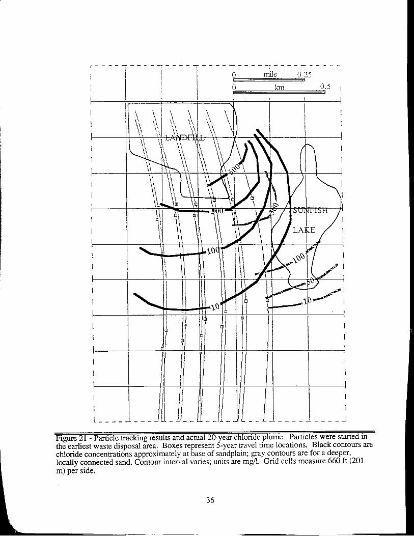
4sI
\\ \),
\\
I
tt\a
II
?lI
@ngresultsandacrual20-yealchlondeplume.Particleswerestartedrnthd earliest waste disposal area. Boxes represent 5-year travel time locations. Black contours are
chloride concentrations approximately at base of sandplain; gray_contours are for a dee^per,.- ^ -
locally connected sand. Contour interval varies; units are mgfl. Grid cells measure 660 ft (201
m) per side.

DiscussionA comparison of the plume's extent with the temporal particle.locations indicates a
discrepancy of at least a fact6r of two, a! thg 20 year old.plume.coincides with the -l0--yearpreOictea piume (Figure 21). Several possibilities may explain the shorter-than-expectedplume-fue a-oont of time-required for ttre iiritiA generation of leachate is uncertail -bqt
probably notinstantaneous. Also unkno*n is the time of travel in the unsaturated 7nne, which is composed ofnatural material and waste. Kimmel and Braids (1930) suggest that four years irre required for the
formation of leachate and its passage through the unsaturated zone; however, this estimate wouldcertainly be subject to climatdeffeils, waste characteristics, and the thickness and properties of the
unsaturited media. In the saturated zone, the downward component of leachate flow increases the
length of the flowpath and therefore decreases the extent of a plume shown in plan view. At the
enSta hndfill, hoivever, this is a fairly insignificant factor when the aquifer thickness is compared
to the plume's extenr. For this reason, the-two'dimensional (o19 layqr) modeling assumption isbe[evdd to be reasonable. Another possibility is that heterogeneities within the outwash may slowthe flow of leachate (MacFarlane and others, 1983).
The history oi ttre contamination source of this srudy creates additional complicating factors
related to the distribution of chloride concentrations 20 years after landfilling commenced. The twomain aspects are the longitudinal dispersion ofthe aq-uifer and the ct,?ngilg contaminant source.
Certainly the chloride al6ng the leading edge of the plumeis affected by disp_ersion; ttrat is, it has
traveled' ster than the avefoge hnear groundwater flbw velocity. ln late 1967,landfill operation-s
began, but the areal extent, -thickness, and composition of the waste has changed a great deal,
esi'e"iitty in the operation's earlier years. The-source concentration therefore has continuallyinireased, as did the surface area of the aquifer receiving percolating leachate. Because the
landfilled waste has gtown in both area and thickness since waste disposal- began, theconcentrations and releaie areas of contaminant tracers have changed significantly, and the value oflongitudinal dispersion cannot be estimated- However, the fact that the waste aispoTl area spread
in t[e direction of groundwater flow, together with the iikelihood of the effect of lon^gitudhaldispersion, suggestihat the plume discrepancy m?y be as great-as. a factor of three or four. If a
*.i." is contiiious and hasi constant ar6a, then th-e longitudinal dispersion of the aquifer may Lre
more easily addressed. Because of its history, the Anoka landfilt does not lend itself to such a
study, and'because of these complicating faciors, the times legu-red.for.leachate generation and
unsa,turatea zone transport cannot be easily or accurately quantified at the Anoka landfill.Evidence of niinimal lateral dispersion is present along the northeast edge of the plume.
This lack of lateral dispersion is in agreement with numerous other studies of contaminants or other
rracers in sandy aquiiers (e.g. RoSertson and others, l99I; Kimmel and Braids, 1980, 1974;Mackay and others, 1986; MacFarlane and others, 1983). Probable_septic inlluencefrom n_ear-bY
homes muddles the contours along the westem edge of the plume (Flickok and Foth & Vry Dy-ke,
1987). Although the monitoring well network at the Anoka landfill is not as dense as at the otherstudy areas m6ntioned above,lhe effect of dispersion in the vertical direction appears to be
negligible." - The orientation of the actual chloride plume differs only slightly from the path predicted byMODPATH (Figure 21). The reason is anributed to a combination of localized effects on the flowfield caused by groundwater interaction with Sunfish Lake with a minor influence from valuesassigned alon! Jpecified-head boundaries. However, given- the positi-on of the landfill on an
assu-med flow fuvide near the confluence of two major rivers, the flow of leachate could have been
thought to have a flow direction ranging anywhere between due south and due east. Thisappliiation of MODPATH is therefore UetieveO to have achieved a fairly accurate prediction of flowdirection.
Selection of additional monitoring well locationsIf ti\e four selected monitoring wells were the only available data for the Anoka landfill,
then no statements could be made regarding the three-dimensional extents of various contaminantplumes. The placement of additional wells at this site, however, could have been guided by an
application of the methodology presented in this paper.
I
3t
--

When locating wells designed to determine the downgradient extent of a contaminant
plume, the numeri.J?"roftr for thi p*ii"A tt"-" should be issumed to be roughty-Yo to f.our
times the actual extenl Literature "*u-prir
orpru-" studies describe negligibfe lateral dispepiolt'
as is the case ar the Anoka landfill. The'lateral histribution of wells may therefore be appropriately
constrained.An understanding of expected plume movement can aid in augmenllq u monitoring well
network. But at the Anoka landfill, snoJJttre network have grown to approximately one hu.ndred
l,irriprir! p"n"r i;;;il;;;; i; increasing_ the netw6rk is to ad&ess those contaminants
that behave different than a conservariv" rolut" suih us chloride. The chloride plume-is important
because contained *itfrin its areal exteniare the pt-umes of chemicals influenceg-by sorption'
;;F"d;;, bt"d"g*eiyr{, "-ia!ton-i.a*tion,
uita ot!"t processes. Detection of light or dense
non-aqueou, pnur"'ifr.uid, iuoura t"quire wells hnished at'the water table or at the base of the
ilu1#, ;,!"o|rilt, ii otoo t-" monito. r the movement of those types of contaminants'
In the enO, thiti"" of a monitoring net*o.k-mqr be tqongll influenced by.public.or
regulatory pr"rr*",iJttt ft""r or pt""iaing"u fictor of safety on the esiimation of the distribution
of released ctremicJi. E;;; in 'ttris ritriti*, a scientifii approach has merit in preventing
haphazard placement 9f monitoring wells'The hydrogeologic enviroimeni-is typic.ally characterized by- t$g! degree of uncertainty'
which makes ""gt"J";i?;;;;trfir airn"irit (Freeze and others,-1990, Massmann and others,
1991). In this study, the extent of conre*aiive-contaminants was estimated without using any of
the abundunt "111oirni-;i
ii6-tp"cinc oata, except for- the heads of four water-table wells'
ffi;g*phf i"t" t * trte -oniioting-n"nuoir. sugg^est a deep sand channel with roughly the same
trend and location as Sunfish Lake. rnii reiture fiis been teimed a tunnel valley / esker complex
bv Hickok and Foti AV;Dyk" trg8zl; ho*"u"., this explanation js not consistent with the
H#ffiGv ,] i*;"ont or tuinel ""il;i; in ttt. regiog, as presented in Figure 6 or bv Quinn
(IggZ). Also, tr,e rilutig"*ir J"t^ fto*G" private"welli of ^the Hunters Hills suMivision south
of Sunfish Lake do not indicate a aeep iumc'ial sand. How an apparent sand-filled channel fits
into the scheme oiiir" gfuriul history of tn" ar91 is open to some debate; it may be. a
paleodrainageway uiro"iui"O with the -Ciantsuurg
sublobe. I-n 1 geotogic framework, where the
unexpected ir uru^uv "*p;;i.d,
such a f*tutr can1inng9 the desig-n of imonitoring well network,
il ii;;piinm how a facies model may suddenly require revision'
38
SUMMARY
Summary, conclusions, and applicationsThis study illustrates the value of detailed surficial geologic mapping in a regional
framework. The mapping of the glacial deposits was performed primarily with low-altitude stereoair-photos and soil surveys. Although the mapping is reconnaissance level inforrration, valuableinformation was obtained for the local study area- Hydrogeologic boundaries and observationpoints were justified because rivers and lakes in the entire local study area were determined to beiituated in pernreable basins. Uniforrr recharge in the modeling area was assumed because of thesimilar geologic units covering the surface.
The two-dimensional geostatistical analysis of the basal elevation of the surficial aquiferexemplifies how abundant, inexpensive information in the form of well logs may refine both ageologic conceptual model and a numerical groundwater tlow model. In this case, the discoveredanisotropy of the surficial aquifer is attributed to south-southeasterly flowing meltwater thatdeposited the sandplain.
The spatially-varying sand/till contact was shown to exert significant control on the flowsystem when compared to the case of an assumed planar aquifer base. This two-dimensionaltechnique has other applications in numerical modeling. For example, the upper and lowerelevations of a confined aquifer could both be kriged in order to determine the geostatistical bestestimates for constraining the thickness of the aquifer in each grid cell. Or, the likelihood ofexistence of a discontinuous confining unit may be analyzed with two-dimensional indicatorgeostatistics (Ritzi, 1991).
The hydrogeologic environment of the local study area is believed to allow fairly accuratemodeling in two dimensions with a minimum of errors resulting from assumptions related toboundary conditions or improper geologic interpretation. Initial hydraulic conductivity estimatesfor the sandplain were determined from grain size analyses to equal approximately 1.2x10⁻³ fvs(3.5x10⁻² cm/s). The effective hydraulic conductivity of the steady-state two-dimensional modelwas calibrated to 2.7x10⁻³ fVs (8.2x10⁻² cm/s) using a literature-based recharge value of 11 in/yr(28 cmlyr). The calibrated conductivity agrees well with values derived from pump tests at thelandfill. The model was found to be sensitive to changes in both hydraulic conductivity andrecharge. One-dimensional analyses of the boundary conditions support the validation of themodel by indicating that l) the assumed flow conditions in the northwest corner of the study areaare possible, and 2) the model is insensitive to short-lived changes in river stages.-
The groundwater flow model could have application in modeling the effects of pumping, ifsuch remediation took place at the landfill. Because the present gnd discretization would notprovide enough resolution for near-site pumping effects, a variable grid would have to bedesigned, with smaller finite difference cells near the landfill. The boundary conditions of thepresent model should suffice, although the effects of boundary conditions are tested best when thesystem is stressed (Franke and Reilly, 1987). If the cone of depression were to approach a
specified-head river boundary, the river leakage package of MODFLOW would need to beimplemented
The actual chloride plume was found to be at least two times shorter than the predicted,particle-nacking plume. This discrepancy is consistent with other examples in the literature (e.g.Kimmel and Braids, 1980; MacFarlane and others, 1983; Robertson and others, L99l). Reasonsfor the difference may include delayed leachate generation and the leachate's time of travel throughthe unsaturated zone. The data at this site are complicated because the composition and thicknessof waste has changed through the years and the area of landfrlled waste has spread in the directionof groundwater flow. The effect of longitudinal dispersion on the flow of contaminants cannot beestimated because of the areally and temporally changing source.
The comparison of the actual chloride plume geometry versus its theoretical extent asdetermined by a particle-nacking analysis is applicable to many hydrogeological studies. Thisdiscrepancy is not mentioned in most texts or papers. In the investigations of Kimmel and Braids(1980), MacFarlane and others (1983), and Robertson and others (1991), hydraulic conductivity
I
-
39

values were obtained using various methods. These case studies suggest the inadequacy of simplyusing "average" hydraulicionductivity values for determining the.transpo.rt of conservative tracers.
tcno-wtedge-of sirctr discrepancies -has
application in remediation investigations, wellheadprotection studies, and other hydrogeologlcal prgjec-ts.' In this investigation, inexpensive ptiUtib-Aomain geologic and hydrglogic info.rmationproduced a flow moA-et that was
-calibrated with-only^four water table monitoring-wells. The
iarticte-t acking resuls matched the actual orientation of tne pll1e quite closely. Jf only these fourinonitoring wefs had existed at this landfill, the locatiorrs of additional wells could have been based
on the prJdictive output of this modeling, with modification based on the common discrepancybetween actual and predicted plume extents.
The findings of this study can serve as a general basis for the design of a threedimensionalmonitoring well nEnvork for an-existing or proposed qotential contamination source. Because thepredicted ilume of a conservative contaminant nacer is typically lyo t9 fo.* ,h:l greater than itsictual extanq downgradient wells may be appropriately l,ocated. The dep$ at which the wells are
screened may be giiaeA by the coniept of do*nward-driven solutes below and near the waste
source, and in abience of iolute contaminants at or near the water-table past a relatively short
distance downgradient. The planning of other monitoring well networks, especially those insimilar hydrogeblogic settings, could benefit from the frndings of case studies such as this.
Becarise this study is not a detailed analysis of the fate and transport characteristics oflandfill leachate, the plumes of other contaminants have not been discussed. By.examining the
chloride data afier twenty years of landfill operations, the inconsistency of predicted vs. actualplumes was addressed foia conservative pollutant tracer. The ctrlori{e plume should represent the
iotthest areal extent of contaminants from such a source. Although the spread of contaminantswith different physical properties should be contained within the pian view.of the chloride plume,relatively deeper or shailower monitoring wells would be necessary to monitor non-aqueousphaseliquids.
- Ultiinately, a monitoring wef network qrfy be augmented as a result -of
regulatoryag'encies and citizens groups desiiing greater confidence on the understanding- of contaminantdistributions. In this iase the place-mEnt of additional wells should be based on a scientificmethodology that incorporates allavailable geological and hydrological information.
Suggestions for further researchOther iase itudies of the relation of monitoring well networks with predicted and actual
plumes would serve ro refine the modeling approach. used il -t!it -paper..- Studies in different
'hydrogeological settings would provide the best-comparisons. A hig.hly detailed three-dimensionalgiouni*atjr modelin-g exercis^e could rely on hydraulic.conductivity values a;sig19d to cellsiccording to a three-&mensional geostatistical characterization,- as-performed b;r lo-nngo.n .a1$Dreiss (1389) for alluvial sedimenls and proposed by Quinn and others (1989) for glacial-driftaquifers. In the present study, however, th9 frydrggeologic environment and boundary conditionswere conduciveio modeling only a surficial aquifer in two dimensions. Other study areas withreasonable three-dimensionll borlndary conditions may allow the opportunity toincorporate suchdsteil, although in a glacial geologic framework both the model construction and the computationaleffort rnay be prohibitive.
tfiis siudy benefitted from a literature-derived recharge rate which could be applieduniformly over ihe modeling area because of the similar outwash-derived soil throughout.Modelinj in other glaciated liations in Minnesota and elsew_here could requ-rc an estimate of the
rechargJrate through surficial till. Daniels and others (199l)-performed.ultiqm analyses^ to
deternine a rechargjrate through an Indiana till, but Helgesen and Lindholm (1977) is one of few-
recharge studies ii Minnesotal Investigations_ of the_iecharge ?ld fracture characteristics ofMinneiota tills would aid in the construction of gtoundwater models ranging in scale from site-
specific to regional, so that recharge input wouldbe.justified by a detailed independent analysis,rather than estimated bv mere model calibration exercises.
4A

REFERENCES
Aller, L., Bennett, T.W., Hacke[, G., Petty, RJ., Lehr, J.H., Sedoris, H., Nielsen, D.M., and Denne, JI., 1989,
Handbook of suggested practices for the desrgn and installation of ground-water monitoring wells: Dublin,Ohio, National Water Well Association,398 p.
Anderson, M.P., 1987a, Treatment of heterogeneities in ground water flow modeling, in Solving ground waterproblems with models: Dublin, Ohio, National Water Well Association, p.444463.
Anderson, M.P., 1987b, Geologic facies models: what can they tell us about heterogeneity?: EOS (AmericanGeophysical Union Transactions), vol. 68(16), p. 300.
Anderson, M.P., 1989, Hydrogeologic facies models to delineate large-scale spatial trends in glacial andglaciofluvial sediments: Geological Society of America Bulletin, vol. l0l, p. 501-511.
Anderson, M.P., and Woessner, W.W., 1992, Applied groundwater modeling: simuliation of flow and advectivetransport New York, Academic Press, 381 p.
Austin, G.S., 1972, Paleozoic lithostratigraphy of southeastern Minnesota: in Sims, P.K., and Morey, G.B.,eds., Geology of Minnesota: a centennial volume: Minnesota Geological Survey, Minneapolis"Minnesota, p.459473.
Bagchi, A., 1990, Design, construction, and monitoring of sanitary landfrll: New York, Wiley, 2U p.
Chambem, L.W., and Bahr, J.M., l992,Trrcer test evaluation of a drainage ditch capture zone: Ground Water, vol.30, no. 5,p.667-675.
Chemicoff, S.8., 1980, The Superior-lobe and Grantsburg-sublobe tills: their compositional variability in east-
central Minnesota [Ph.D. thesis]: University of Minnesota, Minneapolis, 255 p.Chernicoff, S.E., 1983, Glacial characteristics of a Pleistocene ice lobe in east-central Minnesota: Geological
Society of America Bulletin, vol. 94, p. l40l-1414.Clayton, L., and Moran, S.R., 1982, Chronology of late Wisconsinan glaciation in middle North America:
Quaternary Science Reviews, vol. l, p. 55-82.Cooper, W.S., 1935, The history of the upper Mississippi river in late Wisconsin and postglacial time: Minnesota
Geological Bulletin no. 26, I 16 p.
Cravens, SJ., and Ruedisili, L.C., 1987, Water movement in till of east-central South Dakota: Ground Water,vol.25, no. 5, p. 555-561.
Daniels, D.P., Fritz, SJ., and Leap, D.I., 1991, Estimating recharge rates through unsaturated glacial till bytritium tracing: Ground Water, vol.29, no. 1, p. 26-34.
Davis, S.N., Campbell, DJ., Bentley, H.W., and Flynn, T.J., 1985, Ground water tracers: Worthington, Ohio,National Water Well Association, 200 p.
deMarsily, G., 1986, Quantitative hydrogeology: Orlando, Harcourt Brace Jovanovich,440 p.
Englund,8., and Sparks, A., 1988, Geo-EAS (geostatistical environmental assessment software) user's guide: LasVegas, Environmental Monitoring Systems Laboratory, U.S. Environmental Protection Agency,EPA/600/4-88/033.
Ericson, D.W., Lindholm, G-F., and Helgesen,l.O., L974, Water resources of the Rum River watershed east-centralMinnesota: Hydrologic Atlas 509, U.S. Geological Survey.
Eyles, N., 1983, Glacial geology: an inroduction for engineers and earth scienlists: New York, Pergamon hess,409 p.
Eyles, N., and Miall, A.D., 1984, Glacial facies, in Walker, R.G., ed., Facies models (second edition): Toronto,Canada, Geological Association of Canada, p. 15-38.
Farnham, R.S., 1956, Geology of the Anoka sand plain, in Schwartz, G.M., ed., Glacial geology, easternMinnesota Geological Society of America Guidebook for Field Trips, Minneapolis meeting, p.53-&.
Fetter, C.W., 1988, Applied hydrogeology (second edition): Merrill Publishing Co., Columbus, Ohio, 592 p.
Foth & Van Dyke and Associates, Inc., 1987, Anoka regional sanitary landnU, interim studies report, scope I.D.:87W25, October.
Foth & Van Dyke and Associates, Inc., 1989a, Aquifer analysis, Anoka regional saniury landfill, scope I.D.:88W92, May.
Foth & Van Dyke and Associates, Inc., 1989b, Water quality confirmation report, Anoka regional vnitary landfill,scope I.D.: 88W89, May.
Foth & Van Dyke and Associates, Inc., 1990, Construction documentation for monitoring wells MW-34C andMW-35C, Anoka Regional Sanitary Landfill, scope I.D.: 89W79, June.
Franke, O.L., and Reilly, T.E., 1987, The effects of boundary conditions on the steady-stat€ response of threehypothetical glound-water systems - results and implications of numerical expe.riments: U.S.G.S. Water-Supply Paper 2315.
4l

Franke, OI., Reilly, R-8., and Bennett, G.D., 1984, Definition of boundary_and initial_conditions in the analysis' of satgrated ground-water flow systems - an introduction: U.S.G.S. Open-File Report 84458.
Fras€r, F.S., and Bleuer, N.K., 1987, Usebf facies models as predictive tools to locate and ctatacteize aquifers in' glacial rerrains, ln Proceedings of the I{WWA Focus Conference on Midwestern Ground Water Issues:
Dublin, Ohio, National Water Well Association , p. 123-143'Fresze,R.A., and Cherry, J.A.,lgTg,Groundwat€n nentic-e-Halt Inc., Englewood Cliffs' New Jersey, 604 p.
Freeze,,R.A., Massm-i, 1., Smith, L., Sperling, T., and James, B., 1990, Hydrogeological decision analysis: l'a framework Ground Water, vol.28, no.5, p. 738-76f..
Helgesen, J.O., and Lindholm, G F ., lg77 , Geology and waler-supply potential 9f tJre. {gka sand-plain-aquifer'
Minnesota Minnesota Depu of Natural Resources, Division of Waters, Technical Paper No. 6,17 p. --Hendry, MJ., 1982, ffy6tzufi" con'ductivity of a glacial till in Alberta: Ground Water, vol- 20' no. 2, p. 192'192:
i"nOti, MJ.; 1983, HyCroieorogv of clay till in i p'rairie region of Canada Ground Water, vol. 26, no. 5, p' 607-
618.Hickok and Associates, Inc., and Foth & van Dyke and Associates, Inc., 1987, Anoka regional sanitary landfill,
remedial investigation, scope I.D.: 86W69' February.
Hogberg, R.K., 1972, Ground-watel resources in Minnesota in Sims, P.K., and Morey, G.8., eds., Geology of
Minnesota: a centennial volume: Minnesota Geological Suwey, Minneapolis, Minnesota, p- 595.602,
Holtz, R.D., and Kovacs, W.D., 1981, An introduction to geotechnical engineering: Prentice-Hall Inc-'
Englewmd Ctffs, New JerseY, 733 P.Isaaks, g.C.land Srivastava, R.M., 19-89, ep^ptieO geostatistics: New York, Oxford University Press' 561 p.
Jina, M.A., Olsen, B.M., and Bloomgren,-9.4., lgSO, Bedrock geologic and lopgqraphic maps of the seven-- county Twin Cities mefopolitan area, Minnesota: Minnesota Geological Survey Miscellaneous Map
Series, map M-55.Johnson, N.M., and Dreiss, S.M., 1989, Hydrostratigraphic interpretation using indicator geostatistics: Water
Resources Research, vol.25, no. 12, p-2501-2510-Kanivetsiy, R., f989, Bedrock hydrogeology of Hennepin-9o-9nty, in Balaban, N'H' ed' Geologic allas of'
Hlnnepin counry, Minnesta 5l piri, University of Minnesota, Minnesota Geological Survey County
Atlas Series, atlas C4.Kehew, A-8., and passero, R.N., 1990, pH and redox buffering mechanisms in a glacial drift aquifer contaminated
by landfrll leachate: Ground Water, vol- 28, no.5,p-7?3-737 'Kimmel, G.E., and Braids, O.C., Lg}4,Leachate plumes in a highly permeable aquifer: Ground Water, vol- 12,
no. 6, p. 388-393.Kimmel, G.8., and Braids, O.C., 1980, leachate plumes in ground water from Babylon and Islip landfills, Long
Island, New York u.S. Geological Suwey, Professional Paper 1085,38 p.
Knudsen, H.p.; 1988, A short course on geostatistical ore reserve estimation: Montana Tech Division of Mining
and Minerals Engineering, Butte, Montana, 120 p.
Krumbein, W.C., and trl6nt, G.5'.,1943, Permeability as a function of the size parameters of unconsolidated
sand: American Institute of Min. and Met. Eng. Transactions, vol.151 , p. 153-162.
Kuehnast, 8.L., 1978, Climates of the states: Minnesota, iz Ruffner, James A., Climates of the states,
c'limatography of the United States No. 60: Detroit, Gale Research Company, p. 519-540-
Lindgren, nf., iggb,'simulation of ground-water flow in the Prairie du Chien-Jordan and overlying aquifers near'
the Mississippi River, Frid''ley, Minnesota: U.S. Geological Survey, Water-Resources Investigations
Report 904165,152P.fnaiciga, HLA., 1989, An opimizarion approach for groundwater quality monitoring network design: Water
Resource Research, vol. 25, no. 8, p. 177l-1782.MacFarlane, D.S., Cherry, 1.e., Gillhaml R.W., and Sudicky, E.A., 1983, Migration of contaminants in
groundwater at u iananUr'a case study 1. groundwater flow and plume delineation: Journal of Hydrology'
vol. 63, p.1-29.Mackay, D.M., Freyburg, D.L., RoberS, P.V., and Cherry, J.A., 1986, A natural gradient experiment on solute
' 'transport iti u su?lO aquifer l. approach'and overview of plume movemen[ Water Resources Research, vol.
22, no. 13, p. 2017 -2029-Massman, J., and FreEzE,R. A., 1987a, Groundwater contamination from waste management sites: the interaction
between risk-based engineering design and regulatory policy 1. methodology: Water Resources Research'
vol. 23, no. 2, P. 351-367.Massman, J., and preeze,R. A., 1987b, Groundwater contamination from waste management sites: the interaction
between rist-UaseO "ngin""ting
design and regulatory policy 2. results: Water Resources Research, vol.
23,no.2, p. 368-380.
42
d

Massmann, !.,Fr@ze, R.A., Smith, L., Sperling, T., and James, B., 1991, Hydrogeological decision analysis: 2.
applications to ground-water contamination: Ground Waler, vol.29, no.4, p. 536-548.Mast, R.F.; and Potter, P.E.,1963, Sedimentary structures, sand shape fabrics, and permeability II, Journal of
Geology, vol. 71, p. 5a8-565.McDonald, M.G., and Harbaugh, A.W., 1988, A modular three-dimensional finite-difference ground-water flow
model: Techniques of water resources investigations, book 6, chapter A1: Reston, Virginia, U.S.Geological Survey, 528 p.
Mclaughlin, D.B., and Graham, W.D., 1986, Design of cost-effective programs for monitoring ground-water
contamination: IAHS Publ. no. 158, p.307-317.Meyer, P.D., and Brill, E.D. Jr., 1988, A method for locating wells in a groundwater monitoring network under
conditions of uncertainty Water Resource Research, vol.24, no. 8, p. ln7'1282.Mooers, H.D., 1988, Quaternary history and ice dynamics of the late Wisconsin Rainy and Superior lobes, central
Minnesota tPh.D. thesisl: University of Minnesota, Minneapolis,2N p.
Mooen, H.D., 1989, On the formation of tunnel valleys of the Superior lobe, central Minnesota: QuaternaryResearch, vol. 32, p.24-35.
Mooers, H.D., 1990, A glacial-process model: the role of spatial and temporal variations in glacier thermalregime: Geological Society of America Bulletin, vo1.102, p.243-251.
Mossler, 1.H.,1972, Paleozoic structure and stratigraphy of the Twin City region: in Sims, P.K., and Morey,G.B., eds., Geology of Minnesota: a centennial volume: Minnesota Geological Survey, Minneapolis,Minnesota, p.485497.
National Water Well Association / U.Slnvironmental Protection Agency, 1986, RCRA ground water monitoringtechnicat enforcement guidance documen[ Dublin, Ohio, National Water Well Association, 208 p.
Olsen, B.M., and Bloomgren, B.A., 1989, Bedrock geology of Hennepin county, in Balaban, N.H, ed. Geologicarlas of Hennepin county, Minnesota: St. Paul, University of Minnesota, Minnesota Geological SurveyCounty Atlas Series, atlas C4.
Pfannkuch, H.-O., 1975, Study of criteria and models establishing optimum level of hydrogeologic informationfor groundwater basin managemenc Bulletin 81, Water Resources Research Center, University ofMinnesota, Minneapolis, 165 p.
Pfannkuch, H.-O., and Labno, B.A., 1976, Design and optimization of ground-water monitoring networks forpollution studies: Ground Water, vol. 14, no.6, p. 455462.
Pollock, D.W., 1988, Semianalytical computation of path lines for finite-difference models: Ground Water, vol.26, no. 6, p. 743-750.
Pollock, D.W., 1989, Documentation of computer programs to compute and display pathlines using results fromthe U.S. Geological Survey modular three-dimensional finite-difference ground-water flow model:U.S.G.S. Open-File Report 89-381, 188 p.
Potter, P-E., and Mast, R.F., 1963, Sedimentary structures, sand shape fabrics, and permeability I, Journal ofGeology, vol. 71, p- 441471.
Pryor, W.A., 1973, Permeability-porosity patterns and variations in some Holocene sand bodies, AmericanAssociation of Petroleum Geologists Bulletin, vol.57, no.l, p. 162-189.
Quinn, J.J., Mooers, H.D., and Pfannkuch, H.-O., 1989, Groundwater mapping and the optimum amount ofinformation for the assessment of groundwater sensilivity to contamination in complex glacial-driftaquifers: Geological Society of America, Annual Meeting, Absuacts with hograms v. 21, no. 6, p.
Ar92.Quinn, J J., !992, Modeling of groundwater flow, leachate migration, and geostatistical aspects of a portion of the
Anoka sandplain, Minnesota [M.S. thesis]: University of Minnesota, Minneapolis, 158 p.
Quinn, JJ., Barnes, R.J., and Mooers, H.D., 1992, A three-dimensional geostatistical analysis of glacial-driftaquifers and aquitards: Geological Society of America, Annual Meeling, Abstracts with Programs, v.24,no. 7, p. M52-253.
RiEi, R.W., Jr., 1991, Use of indicator geostatistics to quantify heterogeneity of glaciofluvial deposits in buildingmodules for ground water flow and pollution transporf Geological Society of America, North-CentralSection, Abstracts with Programs, p. 56.
Robertson, W.D., Cherry, J.A., and Sudicky, 8.A., 1991, Ground-water contamination from two small septicsystems on sand aquifers: Ground Water, vol.29, no. 1, p. 82-92.
Ruland, W.W., Cherry, J.A., and Feenstra, S., 1991, The depth of fractures and active gtound-water flow in aclayey till plain in southwestern Ontario: Ground Water, vol.29, no. 3., p. 405417.
Schoenberg, M3., 1990, Effects of present and projected ground-water withdrawals on the Twin Cities aquifersystem, Minnesota: U.S. Geological Survey, Water-Resources Investigations Report 90-4001, 165 p.
43

Spruill, T.B., and Candela, L., 1990, Two approaches O design of monitoring networks: Ground Water, vol.28,
no.3, P. 43042.State of Minnesota, 1989, Minnesota Rules 1989, compiled edited, and published by the Revisor of Statutes, State
of Minnesota.Stephenson, D.A., Fleming, A-H., and Mickelson, D.M., 1988, Glacial deposis, iz Back, W., Rosenshein, J.S.,
and Seaber, P3., eds., Hydrogeology: Boulder, Colorado, Geological Society of America, The Geologyof North America, vol. O-2, P. 301-314.
U.S. EPA, 1986, RCRA orientation manual, report no. EPA/530-SW-86-001.Walker, R.G., 1984, General introduction: facies, facies sequences and facies models, in Walker, R.G., ed. Facies
models (second edition): Toronto, Canada, Geological Association of Canada p. 1-9.
Walton, M., 1986, University of Minnesota aquifer heat storage project: STES Newsletter, Earth Sciences
Division, lawrence Berkeley laboratory, University of California vol.8, no.3, p' l-7,Wang, HF., and Anderson, MP., 1982, Infoduction to groundwater modeling: finite difference and finite element
methods: New York, W.H. Freeman and Company,Z31 p.
White, G.W., 1974, Buried glacial geomorphology, in Coatss, DR., ed., Glacial geomorphology: New York,Binghampton, p. 33 L-49.
Williams, R-8., and Farvolden, R.N., 1967, The influence of joints on tle movement of ground water throughglrcrad till: Journal of Hydrology, vol. 5, p. 163-170.
Wright, H-8. Jr., 1973, Tunnel valleys, glacial surges and subglacial hydrology of the Superior Lobe, Minnesotain Black, R.F., Goldthwait, RP., and Willman, G.B., eds.,The Wisconsin Stage: Geological Society ofAmerica Memoir 136, p.251-276
Wright, H.E. Jr., Matsch, C.L., and Cushing, 8.J.,1973, The Superior and Des Moines lobes, in Black, R.F.,
Goldthwait, R.P., and Willman, G.B., eds., The Wisconsin Stage: Geological Society of AmericaMemoir 136, p. 153-185.H.E. Jr.,19?2a, Physiography of Minnesota, in Sims, P.K., and Morey, G.8., eds., Geology ofMinnesota: a centennial volume: Minnesota Geological Survey, Minneapolis, Minnesota, p. 561-578.HE. h.,I972b, Quaternary history of Minnesota, in Sims, P.K., and Morey, G.B., eds., Geology ofMinnesota: a centennial volume: Minnesota Geological Survey, Minneapolis, Minnesota, p. 515-547.
Zheng, C., Wang, H.F., Anderson, MP., and Bradbury, K.R., t988a Analysis of interceptor dirches for controlof groundwater pollution, Journal of Hydrology, vol. 98, p. 67-81.
Zheng, C., -Bradbury, K.R., and Anderson, M.P., 1988b, Role of interceptor ditches in limiting the spread of
contaminants in ground water, Ground Water, vol.26, no. 6, p. 734-742.
Wright,
Wright,