Embed Size (px)
Citation preview
Combining Statistical Intervals and Market Prices: The Worst Case State Price Distribution 1
by
Per Aslak Mykland
TECHNICAL REPORT NO. 553
Department of StatisticsThe University of Chicago
Chicago, Illinois 60637
May 2005
1 This research was supported in part by National Science Foundation grant DMS 02-04639
Some key words and phrases : Incompleteness, Statistical uncertainty, Value at risk.
MSC 2000 Subj. Classif. Primary 60G44, 62F25, 62G15; Secondary 62P05, 62P20.
Running head : The Worst Case State Price Distribution
Combining Statistical Intervals and Market Prices: The Worst Case State Price Distribution 1
by
Per Aslak MyklandThe University of Chicago
Abstract
The paper shows how to combine (historical) statistical data and
(current) market prices to form conservative trading strategies for options.
This gives rise to a “worst case” state price distribution, which provides
sharp price bounds for all convex European options.
1 This research was supported in part by National Science Foundation grant DMS 02-04639.
Some key words and phrases : Incompleteness, Statistical uncertainty, Value at risk.
MSC 2000 Subj. Classif. Primary 60G44, 62F25, 62G15; Secondary 62P05, 62P20.
Running head : The Worst Case State Price Distribution
1
1. Introduction. The pricing and hedging of options usually presupposes a known proba-
bility distribution P for the price S of the underlying security. When P is not known, one approach
is to find a prediction set for, say, the volatility of S, and then to hedge in such a way that the
option liability is covered whenever the prediction set is realized (Avellaneda, Levy and Paras
(1995), Lyons (1995), Mykland (2000, 2003a)). This procedure, however, fails to take account of
the values of market traded options on the same security. This paper will show in the context of
convex European options that such values can be incorporated in a uniform manner with the help
of what we term a worst case distribution. The development is related to earlier work by Bergman
(1996), Frey and Sin (1999), Frey (2000) and Mykland (2003b).
To describe our results in this paper, we begin with the cast:
(i) The securities that are traded in the market:
• S = (St)0≤t≤T , the price process of a stock that pays no dividend.
• Λ = (Λt)0≤t≤T , the price of a zero coupon bond maturing at T, with value one dollar (or euro,
or yuen, or krone).
• European call and put options maturing at T (see Section 2.1).
We can think of the value S∗t = St/Λt as the price of a forward contract on the stock S with
maturity T . We shall assume that S∗ is governed by an unknown probabilty P which belongs to
a class Q of distributions. The main requirement on P is that S∗ be an Ito process
dS∗t = µtS
∗t dt + σtS
∗t dW ∗
t (1.1)
where (µt) and (σt) are random processes and (W ∗t ) is a Wiener process.
(ii) A prediction bound on the volatility σ2t , in the form of a prediction interval IΞ+
IΞ+
= (σt) :
∫ T
0σ2
udu ≤ Ξ+. (1.2)
(iii) A European payoff g(ST ) to be made at time T , where g will mostly be taken to be convex.
The problem we wish to solve is the following. We look for a process (Vt) with two properties.
Vt must be the value of a self financing dynamic portfolio in the market traded securities (see Section
2.2 for the definition of this concept). Also, VT must cover the option liability if the prediction set
2
is realized, i.e.,
VT ≥ g(ST ) P − a.s. on IΞ+
, for all P ∈ Q. (1.2a)
In particular, we wish to find the amount V0(g) which is the smallest starting value for for such a
self financing portfolio:
Definition. The quantity V0(g), provided it exists, will be called the conservative starting
value for prediction set IΞ+
and payoff g(ST ) at T .
A similar setup involving more general prediction sets and market traded securities is given
in Mykland (2003a), which discusses the relevant concepts in some detail.
What is special about the development in the current paper is that we show the existence of
a mapping from the prediction bound Ξ+ to a cumulative distribution F Ξ+
on ST :
Ξ+ → FΞ+
(1.3)
so that for all (non strictly) convex g which do not grow too fast, the conservative starting value
for prediction set IΞ+
and payoff g(ST ) at T is
V0(g) = Λ0
∫g(s)dFΞ+
(s). (1.4)
In other words: there is one F Ξ+
which can be taken as the worst case state price distribution
for all convex payoffs g(ST ). Convex options includes calls and puts.
FΞ+
is what we call the worst case distribution for for the market structure and prediction
set described above. In consequence, since F Ξ+
is independent of the payoff function g, one does
not need to compute the value V0(g) for each g, but instead can find the distribution F Ξ+
. Also,
a distribution function is a more conceptual object. F Ξ+
is a state price distribution in the sense
used in finance, see, for example, Duffie (1996).
3
2. Description and main theorem.
2.1. The worst case distribution. For reasons of mathematical convenience, assume that all
market traded options are European puts. This is no restriction on results, as puts and calls can
be converted to each other via put-call parity, see Chapter 7.4 (pp. 174-175) of Hull (2003). In
practice, one would want to take the most liquid of the put and the call to minimize the transaction
cost. A put option with strike price K has value (K − ST )+ at maturity T . Its market price at
time t will be denoted by P Kt , and for the discounted quantity, we use P K∗
t = PKt /Λt. A discussion
of a formulation in terms of calls is given in Section 8.
We suppose that the market traded puts have strike prices K1, ...,Kq .
To describe F Ξ+
, introduce the standardized process
dSt = StdWt, S0 = S∗0(= S0/Λ0) (2.1)
where W is a standard Brownian motion. The corresponding probability distribution will be called
P . Then
FΞ+
(s) = P (Sτ∧Ξ+ ≤ s) (2.2)
where
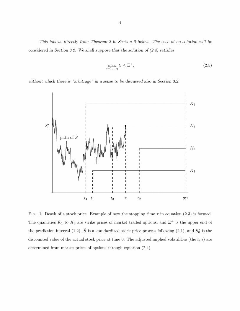
τ = inft : t ≥ ti and Sτ = Ki for some i, 1 ≤ i ≤ q (2.3)
and where the t1, ..., tq are nonrandom, independent of Ξ+, and the solution of
E(Ki − Sτ )+ = PKi
0 /Λ0 1 ≤ i ≤ q (2.4)
where the left hand side of (2.4) is taken as a function of the tis through (2.3). A display illustrating
how τ is formed is given in Fig. 1.
Definition. The ti’s given by (2.1) and (2.3-(2.4) will be called adjusted (cumulative)
implied volatilities. (Compare to Section 3.1). The worst case (state price) distribution F Ξ+
is
then as given by (2.2).
Proposition 1. If (2.3)-(2.4) has a solution, it is unique.
4
This follows directly from Theorem 2 in Section 6 below. The case of no solution will be
considered in Section 3.2. We shall suppose that the solution of (2.4) satisfies
maxi=1,...,q
ti ≤ Ξ+, (2.5)
without which there is “arbitrage” in a sense to be discussed also in Section 3.2.
.
.
.
.
.
.
.
.
.
.
.
.
.
.
.
.
..
.
.
.
.
.
.
.
.
.
..
.
.
.
.
.
.
.
.
.
.
.
.
.
.
.
.
.
.
.
.
.
.
.
.
.
.
.
.
.
.
.
.
.
.
.
.
.
.
.
.
.
.
.
.
.
..
.
.
.
.
.
.
.
.
.
.
.
.
.
.
.
.
.
.
.
.
.
.
..
.
..
.
.
.
.
.
..
.
.
.
.
.
.
.
.
.
.
.
.
.
.
.
.
.
.
..
.
.
.
.
.
.
.
.
.
.
.
.
.
.
.
.
.
.
.
.
.
.
.
.
.
.
.
.
..
.
.
.
.
.
.
.
.
.
.
.
..
.
..
.
.
.
.
.
.
.
.
.
.
.
.
.
..
.
.
.
.
.
.
.
.
.
.
..
.
.
.
.
..
.
.
.
.
.
.
.
.
.
.
.
.
.
.
.
.
.
.
.
.
.
.
.
..
.
.
.
.
.
.
.
.
.
.
.
.
.
.
.
.
.
.
.
.
.
.
.
.
.
..
.
.
.
.
.
.
.
.
.
.
..
.
.
.
.
.
.
.
.
.
.
.
.
.
.
.
.
.
.
.
.
.
.
.
.
.
.
.
.
..
.
.
.
.
.
..
.
.
.
..
.
.
.
.
.
.
.
.
.
.
..
.
.
.
.
.
.
.
.
.
..
.
.
.
.
.
.
.
.
.
.
.
.
.
.
.
.
.
.
.
.
.
.
.
.
.
.
.
.
.
..
.
.
.
.
.
.
.
.
.
.
.
.
.
.
.
.
.
.
.
.
.
.
.
.
.
.
.
.
.
.
.
.
.
.
.
.
.
.
.
.
.
.
.
.
.
.
..
.
.
.
.
.
.
.
.
.
.
.
.
.
.
.
.
.
.
.
.
..
.
.
.
.
.
.
.
.
.
.
.
.
..
.
.
.
.
.
.
.
.
..
.
.
..
.
.
.
.
.
.
.
.
.
.
.
..
.
.
.
.
.
.
..
.
.
.
.
.
.
.
.
.
.
.
.
.
.
.
.
.
.
.
..
.
.
.
.
.
.
.
.
.
..
.
.
.
.
.
.
.
.
.
..
.
.
.
.
.
.
.
.
.
.
.
.
.
.
.
.
.
.
.
.
.
.
.
.
.
.
.
.
.
.
.
.
.
.
.
.
.
.
.
.
.
.
.
.
.
.
.
.
.
.
.
.
.
.
.
.
.
.
.
.
.
.
.
..
.
.
.
.
.
.
.
.
.
.
.
.
.
.
.
.
.
.
.
.
..
.
.
.
.
.
.
..
.
.
.
.
.
.
.
.
.
.
.
.
.
.
..
.
.
.
.
.
.
.
.
..
.
.
.
.
.
.
.
.
.
.
..
.
.
.
.
..
.
..
.
.
.
.
.
.
.
.
.
..
.
.
.
.
.
.
.
.
.
.
.
.
.
.
.
.
.
..
.
.
.
.
.
.
.
..
.
.
.
.
.
..
.
.
.
.
.
.
.
..
.
.
.
.
.
.
.
.
.
..
.
.
.
.
.
.
.
.
.
.
.
.
..
.
.
.
.
.
.
.
.
.
.
.
..
.
.
.
.
.
.
.
.
.
.
.
.
..
.
.
.
.
.
....
.
.
.
.
.
.
.
.
.
.
.
.
.
.
..
.
.
.
.
.
.
.
.
.
.
.
.
.
.
..
.
.
.
.
.
.
..
.
.
.
.
.
.
.
.
.
.
.
.
.
.
.
.
.
.
.
.
..
.
.
.
.
..
.
.
.
.
.
.
.
.
.
.
.
..
.
..
.
.
.
.
.
.
.
.
.
.
.
.
.
.
.
.
.
.
..
.
.
.
.
.
.
.
..
.
.
.
.
.
.
.
.
.
.
.
.
.
.
.
.
.
.
.
.
.
.
.
.
..
.
.
.
.
.
.
.
.
.
.
.
.
.
.
.
.
..
.
.
..
.
.
.
..
.
..
.
.
.
.
.
.
.
.
.
..
.
.
.
.
.
.
.
.
.
.
.
..
.
.
.
.
.
.
.
.
.
.
.
.
.
.
.
.
.
.
.
.
.
.
.
.
.
.
.
.
.
.
.
.
.
.
.
.
.
..
.
.
.
.
.
.
.
.
.
..
.
.
.
.
.
.
.
.
.
.
.
.
.
.
.
.
.
.
.
.
.
.
.
.
.
.
.
.
.
..
.
.
..
.
.
.
.
.
..
.
.
.
.
.
.
.
.
.
.
.
.
.
.....
.
.
.
.
.
..
.
.
.
.
.
.
.
.
.
.
.
.
.
.
.
.
.
.
.
.
.
.
.
.
.
.
.
.
.
.
.
.
.
.
.
.
.....
.
.
.
.
.
.
.
.
.
.
.
.
.
.
.
..
.
.
.
.
.
.
.
.
.
.
.
.
.
.
.
.
.
..
.
.
.
.
.
.
.
.
.
.
.
.
..
.
.
.
.
.
.
.
.
.
.
.
.
.
.
.
.
..
.
.
.
.
.
.
.
.
.
.
.
.
.
.
.
.
.
.
.
.
.
.
.
.
.
.
.
..
.
.
.
.
.
.
.
.
.
.
.
.
.
.
.
.
.
.
.
.
.
.
.
..
.
.
.
.
.
.
.
.
.
.
.
.
.
.
.
..
.
.
..
.
.
.
.
.
.
.
.
.
.
.
.
.
.
.
..
..
.
.
.
.
.
.
.
.
.
.
.
.
.
.
..
.
.
.
.
..
.
.
.
.
..
.
.
.
..
.
.
.
.
.
.
.
.
.
..
.
.
.
.
.
.
.
.
.
..
.
.
.
.
.
..
.
.
.
.
.
.
.
.
.
.
.
.
.
.
.
.
.
.
.
.
.
.
.
.
.
.
.
.
..
.
.
.
.
..
.
.
..
.
.
.
.
.
.
.
.
.
.
.
.
.
.
.
.
.
.
.
.
.
.
.
..
.
.
.
.
.
.
.
.
.
.
.
.
.
.
.
..
.
.
.
.
.
.
.
.
.
.
.
.
.
.
.
.
..
.
.
.
.
.
.
.
.
.
.
.
.
.
.
.
.
.
.
.
.
.
.
.
.
.
.
.
.
.
..
.
.
.
.
.
.
.
.
.
.
.
.
.
.
.
.
.
.
.
.
.
.
.
..
..
.
.
.
.
.
.
.
.
.
.
.
.
.
.
.
.
.
....
.
.
.
.
.
.
..
.
.
.
.
.
.
.
.
.
.
.
.
.
.
.
.
.
.
.
.
.
.
.
.
.
.
.
.
.
.
.
.
.
.
.
.
.
.
.
.
..
.
.
.
.
.
.
.
.
.
.
.
.
.
.
.
..
..
.
.
.
.
.
.
.
..
.
.
.
.
.
.
.
.
.
.
.
.
.
.
.
..
.
.
.
..
.
.
.
.
.
.
.
.
.
.
.
.
.
.
.
.
.
.
.
.
.
.
.
..
.
.
.
.
.
.
.
.
..
.
.
.
.
.
.
.
.
.
.
.
.
.
..
.
.
.
.
.
.
.
.
.
.
.
.
.
.
.
.
.
.
..
.
.
.
.
.
.
.
..
.
.
.
.
.
.
.
.
.
.
.
.
..
.
.
..
.
.
.
.
.
.
..
.
.
.
.
.
.
.
.
.
.
.
.
.
.
.
.
.
.
.
.
..
.
.................................................................................................................................................................................................................................................................................................................................................................................................................................................................................................................................................................................................................................................................................................................................................................................................................................................................................................................................................................................................................................................................................................................................................................................................................................................................................................................................................................................................................................................................................................................................................................................................................................................................................................................................................................................................................................................................................................................................................................................................................................................................................................................................................................................................................................................................................................................................................................................................................................................................................................................................................................................................................................................................................................................................................................................................................................................................................................................................................................................................................................................................................................................................................................................................................................................................................................................................................................................................................................................................................................................................................................................................................................................................................................................................................................................................................................................................................................................................................................................................................................................................................................................................................................................................................................................................................................................................................................................................................................................................................................................................................................................................................................................................................................................................................................................................................................................................................................................................................................................................................................................................................................................................................................................................................................................................................................................................................................................................................................................................................................................................................................................................................................................................................................................................................................................................................................................................................................................................................................................................................................................................................................................................................................................................................................................................................................................................................................................................................................................................................................................................................................................................................................................................................................................................................
......................................................................................................................................................................................................................................................................................................................................................................................................................................................................................................................................................................................................................
.................................................................................................................................................................................................................................................................................................................................................................................................................................................................................................................................................................................................................................................................
...........................................................................................................................................................................................................................................................................................................
............................................................................................................................................................................................................................................................................................................................................................................................................................................................................................................................................................................................................................................................................................................................................................................................................................................................................................................
.
.
.
.
.
.
.
.
.
.
.
.
.
.
.
.
.
.
.
.
.
.
.
.
.
.
.
.
.
.
.
.
.
.
.
.
.
.
.
.
.
.
.
.
.
.
.
.
.
.
.
.
.
.
.
.
.
.
.
.
.
.
.
.
.
.
.
.
.
.
.
.
.
.
.
.
.
.
.
.
.
.
.
.
.
.
.
.
.
.
.
.
.
.
.
.
.
.
.
.
.
.
.
.
.
.
.
.
.
.
.
.
.
.
.
.
.
.
.
.
.
.
.
.
.
.
.
.
.
.
.
.
.
.
.
.
.
.
.
.
.
.
.
.
.
.
.
.
.
.
.
.
.
.
.
.
.
.
.
.
.
.
.
.
.
.
.
.
.
.
.
.
.
.
.
.
.
.
.
.
.
.
.
.
.
.
.
.
.
.
.
.
.
.
.
.
.
.
.
.
.
.
.
.
.
.
.
.
.
.
.
.
.
.
.
.
.
.
.
.
.
.
.
.
.
.
.
.
.
.
.
.
.
.
.
.
.
.
.
.
.
.
.
.
.
.
.
.
.
.
.
.
.
.
.
.
.
.
.
.
.
.
.
.
.
.
.
.
.
.
.
.
.
.
.
.
.
.
.
.
.
.
.
.
.
.
.
.
.
.
.
.
.
.
.
.
.
.
.
.
.
.
.
.
.
.
.
.
.
.
.
.
.
.
.
.
.
.
.
.
.
.
.
.
.
.
.
.
.
.
.
.
.
.
.
.
.
.
.
.
.
.
.
.
.
.
.
.
.
.
.
.
.
.
.
.
.
.
.
.
.
.
.
.
.
.
.
.
.
.
.
.
.
.
.
.
.
.
.
.
.
.
.
.
.
.
.
.
.
.
.
.
.
.
.
.
.
.
.
.
.
.
.
.
.
.
.
.
.
.
.
.
.
.
.
.
.
.
.
.
.
.
.
.
.
.
.
.
.
.
.
.
.
.
.
.
.
.
.
.
.
.
.
.
.
.
.
.
.
.
.
.
.
.
.
.
.
.
.
.
.
.
.
.
.
.
.
.
.
.
.
.
.
.
.
.
.
.
.
.
.
.
.
.
.
.
.
.
.
.
.
.
.
.
.
.
.
.
.
.
.
.
.
.
.
.
.
.
.
.
.
.
.
.
.
.
.
.
.
.
.
.
.
.
.
.
.
.
.
.
.
.
.
.
.
.
.
.
.
.
.
.
.
.
.
.
.
.
.
.
.
.
.
.
.
.
.
.
.
.
.
.
.
.
.
.
.
.
.
.
.
.
.
.
.
.
.
.
.
.
.
.
.
.
.
.
.
.
.
.
.
.
.
.
.
.
.
.
.
.
.
.
.
.
.
.
.
.
.
.
.
.
.
.
.
.
.
.
.
.
.
.
.
.
.
.
.
.
.
.
.
.
.
.
.
.
.
.
.
.
K1
K2
K3
K4
t4 t1 t3 t2
•
τ Ξ+
S∗0
path of S
Fig. 1. Death of a stock price. Example of how the stopping time τ in equation (2.3) is formed.
The quantities K1 to K4 are strike prices of market traded options, and Ξ+ is the upper end of
the prediction interval (1.2). S is a standardized stock price process following (2.1), and S∗0 is the
discounted value of the actual stock price at time 0. The adjusted implied volatilities (the ti’s) are
determined from market prices of options through equation (2.4).
5
2.2. Trading strategies: Theoretical considerations. We define the class Q given the initial
discounted values S∗0 and P Ki∗
0 , 1 ≤ i ≤ q, as follows:
Definition. Q is a collection of distributions on the set of functions Ω = C[0, T ]×D[0, T ]q ,
and (S∗t , PK1∗
t , ..., PKq∗
t ) is the coordinate process. Every P ∈ Q must satisfy (1.1), and the
coordinate process must have the correct initial value (S∗0 , PK1∗
0 , ..., PKq∗
0 ) with probability one.
Also, for given P , the process (σt) must be bounded P -a.s. (but one does not need to know
the bound). Finally, each P must be mutually absolutely continuous with a P ∗ under which the
coordinate process is a martingale. The collection of such P ∗s will be called Q∗.
The requirement of equivalence to a “risk neutral measure” P ∗ is the most convenient way to
avoid arbitrage opportunities in the market. Not only is S∗ a martingale under P ∗, but processes
PKi can be found, with correct initial value P Ki
0 , such that P Ki∗ is a martingale.
The filtration describing the market will be called (Ft) and can be any that is right continuous,
and which makes the coordinate process adapted and martingales under all P ∗ ∈ Q∗. This (Ft)
can be either the smallest filtration with these properties, or anything bigger satisfying the same
criteria, such as the “analytic completion” discussed in Mykland (2003a). The latter is particularly
useful from a statistical perspective. A precise discussion of the conceptual issues involved can be
found in Sections 2, 3.2 and 4 of this earlier paper. – All processes are taken to be cadlag and
adapted to (Ft).
A self financing dynamic portfolio (Vt), with discounted value V ∗t = Vt/Λt, is defined as a
process which, for any P ∈ Q, can be represented by V ∗ = H∗ − D∗, where D∗ is non decreasing
(“dividend”), and H∗ is a stochastic integral with respect to S∗ and the P Ki∗. Stochastic integrals
are as defined in Chapter I.4d (pp. 46-51) of Jacod and Shiryaev (2003). The random variables
H∗−λ must be uniformly integrable for all P ∗ ∈ Q∗, where the λ describe the set of stopping
times taking values in [0, T ].
We can confine ourselves to considering discounted quantities by virtue of numeraire invari-
ance, see Chapter 6 of Duffie (1996). In the current situation where we discount by the zero coupon
bond Λ, FΞ+
and the option liabilities g(ST ) and (K−ST )+ also only depend on discounted quan-
tities, since ST = S∗T . All conditions, therefore, can and are directly imposed on the discounted
6
processes. The author learned this device from the paper of El Karoui, Jeanblanc-Pique, and
Shreve (1998).
The uniform integrability condition is intended to avoid doubling strategies, cf. Chapter 6.B
of Duffie (1996), and p. 670 of Mykland (2000). For other discussions of self financing trading
strategies, see Harrison and Kreps (1979), Harrison and Pliska (1981), Chapter 6 of Duffie (1996),
and, in the context of super-hedging, Cvitanic and Karatzas (1992, 1993), El Karoui and Quenez
(1995), Eberlein and Jacod (1997), Karatzas (1996), Karatzas and Kou (1996), Kramkov (1996),
and Follmer and Leukert (1999, 2000).
2.3. Form of the self financing portfolio. The trading strategy that starts with V0(g) only
requires a static position in the market traded options. We explain this in the following.
At the outset of trading, suppose one takes a position of λi units in the put option with strike
price Ki. We let this position be static, in the sense that we hold it without change until expiry
at time T . The problem then changes to that of covering a liability of the form hλ(ST ), where
hλ(s) = g(s)−q∑
i=1
λi[(Ki − s)+ − PKi∗0 ]. (2.6)
This is since a loan of P K0 dollars at time 0 requires a repayment of P K∗
0 dollars at maturity.
The two problems are equivalent, and V0(hλ) = V0(g). It turns out, however, that there is
one value of λ = (λ1, ..., λq) so that the dynamic hedge for liability hλ(ST ) only involves trading
in the forward contract S∗ (in other words, H∗ is a stochastic integral over S∗ only).
Practically, this is important because transaction costs are normally higher in the market
traded options than in the forward contract S∗ (which, if need be, can be created by securities S
and Λ). We otherwise ignore the issue of trading cost in this paper.
7
2.4. The main result.
Theorem 1. Assume that (2.3)-(2.4) has a solution. Also suppose (2.5). Then there exists
a mapping (1.3) so that for all (non strictly) convex g satisfying |g(s)| ≤ a + bs2−ε for some ε > 0,
the conservative starting value V0(g) for prediction set IΞ+
and payoff g(ST ) at T exists and is
given by (1.4). F Ξ+
is given by (2.2) above. There is a trading strategy that starts with value
V0(g), and only requires a static position in the market traded options, as described in Section 2.3
above.
The theorem is proved in the Appendix. – The general issue of how to compute the worst
case distribution and its corresponding hedging strategy is discussed below in Section 7. First,
however, an interpretation of the tis.
3. Implied volatilities, and arbitrage. Note first that the construction in Section 2.1 is
a conversion of time to volatility scale. The ti’s can be seen as a form of implied volatilites. First,
consider the case where this is exactly true.
3.1. Connection to implied volatility. The Black-Scholes (1973)-Merton (1973) form of the
price at time 0 of a European put option with strike K is BSMP (S0,− log Λ0, σ2T ), where
BSMP (S,R,Ξ) = K exp(−R)Φ(−d2)− SΦ(−d1)
with
d1,2 = (log(S/K) + R ± Ξ/2) /√
Ξ,
and where the instantanouos volatility σ2t is taken to be constant and equal to σ2. Also, Φ is the
standard normal cumulative distribution function.
Of course, the model underlying this formula may not be valid, and prices do not generally
behave as if it were, see for example Hull (2003), but it is customary to invert the function to find
so-called implied volatilities. We shall here do this on the cumulative scale.
Definition. The (cumulative) implied volatility at time zero for strike price K, ΞK , is
defined by
BSMP (S0,− log Λ0,ΞK) = PK0
8
It is also natural to call the ti from Theorem 1 the conditional (cumulative) implied volatility at
time zero for strike price Ki. For both objects, we omit “cumulative” unless this is not clear from
the context.
The first connection to F Ξ+
is now as follows.
Example 1. If all traded options have the same implied volatility:
ΞK1= ... = ΞKq ,
then
t1 = ... = tq = ΞK1
This is easily seen from Theorem 1. In the more general case of unequal implied volatilities,
argmini(ti) = argmini(ΞKi) (there can be several such i’s, or course) and ti and ΞKi
must coincide
for these indices i. Also, one can see more generally from the convexity of the put payoff that
ti ≥ ΞKi.
3.2. The tis and arbitrage. Arbitrage is the construction of a self financing strategy which
makes a profit for some P ∈ Q, and which does not lose money almost surely, for all P ∈ Q. For
issues related to the avoidance of doubling strategies, see Chapter 6 of Duffie (1996).
There are two ways that arbitrage can occur in our setting. One is if (2.5) is violated. The
other is if the system (2.3)-(2.4) has no solution. The latter case is the most clear cut (with proof
in the Appendix):
Proposition 2. If (2.3)-(2.4) has no solution, then there is arbitrage.
The former case is one of “statistical arbitrage”, in the sense that the prediction interval IΞ+
has to be realized, otherwise a loss can occur.
Proposition 3. Assume that (2.3)-(2.4) has a solution, but that maxi=1,...,q ti > Ξ+. Then
there is a trading strategy which, provided IΞ+
is realized, yields a positive return of at least c∗ at
time T , almost surely for any P ∈ Q. Here c∗ is a positive constant independent of P .
9
Proof of Proposition 3. Let S be the indices for which the tis are smaller than Ξ+, and let
I be the index i corresponding to the smallest ti strictly greater than Ξ+. We shall be interested
in earning money on the put payoff g(s) = (KI − s)+. The following argument remains valid if S
is empty.
Note that the ti, i ∈ S, solve (2.3)-(2.4) for this index set. Let V0(g) be the price given by
Theorem 1 based on hedging in S, Λ and the puts with strike Ki, i ∈ S. Our claim is now that
V0(g) < P KI
0 . (3.1)
Thus, one can sell the option with payoff g(ST ), start a self financing trading strategy with initial
value V0(g), and be sure that the liability is covered so long as IΞ+
is realized. The profit is at
least c = P KI
0 − V0(g), if taken at time 0, or c∗ = c/Λ0 if taken at time T (any random additional
profit has, of course, to be taken at time T ).
To see (3.1), let τ be given on the form (2.3) based on ti, i ∈ S ∪ I. Also let K− =
supKi < KI , i ∈ S and K+ = infKi > KI , i ∈ S. Let C = τ ≥ Ξ+ and SΞ+ ∈ (K−,K+).
It then follows that
PKI
0 − V0(g) = E[g(Sτ ) − g(Sτ∧Ξ+)] = E[X],
where X is zero outside C, and otherwise positive.
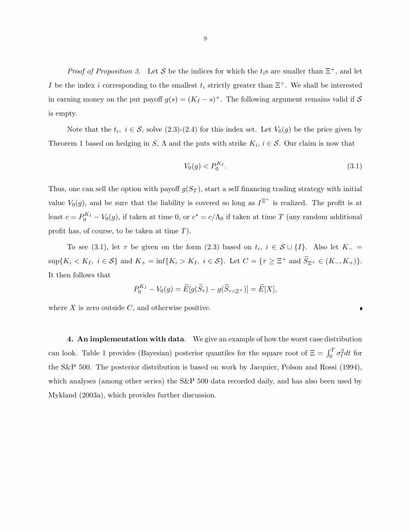
4. An implementation with data. We give an example of how the worst case distribution
can look. Table 1 provides (Bayesian) posterior quantiles for the square root of Ξ =∫ T0 σ2
t dt for
the S&P 500. The posterior distribution is based on work by Jacquier, Polson and Rossi (1994),
which analyses (among other series) the S&P 500 data recorded daily, and has also been used by
Mykland (2003a), which provides further discussion.
10
Table 1
S&P 500: Posterior distribution of Ξ =∫ T0 σ2
t dt for T = one year
posterior coverage 50% 80% 90% 95% 99%
upper end√
Ξ+ .168 .187 .202 .217 .257of posterior interval
The posterior is conditional on log(σ20) taking the value of the long run mean of log(σ2).
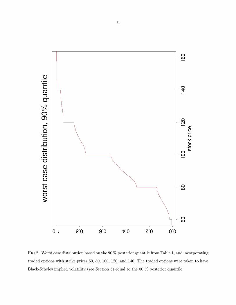
We now assume that market traded options are available for a certain number of strike prices.
For a given set of securities prices, a worst case distribution given in Fig. 2, corresponding to the
90 % posterior quantile. A comparison of the worst case distribution for different quantiles is given
in Fig. 3.
11
wors
t cas
e di
strib
utio
n, 9
0% q
uant
ile
stoc
k pr
ice60
8010
012
014
016
0
0.00.20.40.60.81.0
Fig 2. Worst case distribution based on the 90 % posterior quantile from Table 1, and incorporating
traded options with strike prices 60, 80, 100, 120, and 140. The traded options were taken to have
Black-Scholes implied volatility (see Section 3) equal to the 80 % posterior quantile.
12
wors
t cas
e di
strib
utio
n
stoc
k pr
ice60
8010
012
014
016
0
0.00.20.40.60.81.0
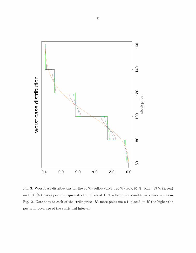
Fig 3. Worst case distributions for the 80 % (yellow curve), 90 % (red), 95 % (blue), 99 % (green)
and 100 % (black) posterior quantiles from Tabled 1. Traded options and their values are as in
Fig. 2. Note that at each of the strike prices K, more point mass is placed on K the higher the
posterior coverage of the statistical interval.
13
5. Asymptotic form of the worst case distribution. As can be seen in Fig. 2-3,
the shape of the continuous part of the distribution has a characteristic form. We here give the
asymptotic form of this shape.
Proposition 4. Suppose that (2.3)-(2.4) has a solution, and let (2.5) be satisfied. Then,
for 1 ≤ i ≤ q − 1, and Ki < s < Ki+1, and as Ξ+ → ∞,
d
dsP (Sτ∧Ξ+ ≤ s | Ki < Sτ∧Ξ+ < Ki+1) = cs−3/2 sin
(π
log(s/Ki)
log(Ki+1/Ki)
)+ o(1), (5.1)
where
c−1 = (K1/2i + K
1/2i+1) bi /
(b2i +
1
4
)(5.2)
and bi = π/ log(Ki+1/Ki). Similarly, at the edges, both dP (Sτ∧Ξ+ ≤ s | St1 and Sτ∧Ξ+ < K1)/ds
and dP (Sτ∧Ξ+ ≤ s | St1 and Sτ∧Ξ+ > Kq)/ds have the form
c′s−3/2(t− t1)−1/2
∣∣∣∣∣φ(
log(s/St1)
(t − t1)1/2
)− φ
(log(s/K1 or q) + log(St1/K1 or q)
(t − t1)1/2
)∣∣∣∣∣
on the respective sets 0 < s < K1, St1 < K1, t > t1 and s > Kq, Stq > Kq, t > tq, and are
otherwise zero. Here, the proportionality constant depends on St1 . Also, obviously, “K1 or q” is
K1 for the lower edge and Kq for the upper edge.
6. Finding t1, ..., tq: the general case.. We here present algorithms for finding the
conditional implied volatilities. Set P K∗t = PK
t /Λt. In other words, this is the discounted put price
at t. We start by characterizing the output, and the algorithms are stated just after the Theorem.
Theorem 2.
(a) Algorithms 1 and 2 yield the same result.
(b) (2.3)-(2.4) has a solution if and only if either algorithm does not return a “no solution”
message.
(c) In the absence of a “no solution” message, the output of either algorithm is unique, and
satisfies (2.3)-(2.4).
(d) If (2.3)-(2.4) has a solution, then it is unique, and is provided by either algorithm.
14
Obviously, one of statements (b) and (d) is redundant given (c), but it seemed to improve
readability to have them both there. The result is proved in the Appendix. Recall that the case
of no solution to (2.3)-(2.4) has been discussed in Proposition 2 above.
Before going to the two main algorithms, we give the core component of both as Algorithm
0. At the end of the section, we show some more detail on how to compute Step 1 in the following.
Algorithm 0. We use an index set S ⊆ 1, ..., q, where index i corresponds to Ki, PKi∗0 ,
and ti. tj’s where j is not in S have either already been found, or are irrelevant. Also, a provisional
version of τ is given.
(0) If, for any i ∈ S, E(Ki − Sτ )+ ≤ PKi∗
0 , then the algorithm terminates with a “no solution”
message. Otherwise:
(1) For i ∈ S, find ti by:
E(Ki − Sτ∧ti)+ = PKi∗
0 .
(2) Remove all i corresponding to the smallest ti from S (there can be ties between the is).
(3) Set
τ = inft : t ≥ ti and Sτ = Ki for i not in S
The algorithms described in Theorem 2 are then given by
Algorithm 1. Finds t1, ..., tq in accordance with Theorem 2. This is the loop version. If any
option value is non-positive, the algorithm terminates with a “no solution” message. Otherwise,
set initial values: S = 1, ..., q and τ = +∞. Then
Loop:
Go through Steps 0-3 in Algorithm 0
Repeat loop until S is empty (unless Step 0 has triggered early termination)
For aficionados of recursion, an alternative scheme would be the following.
15
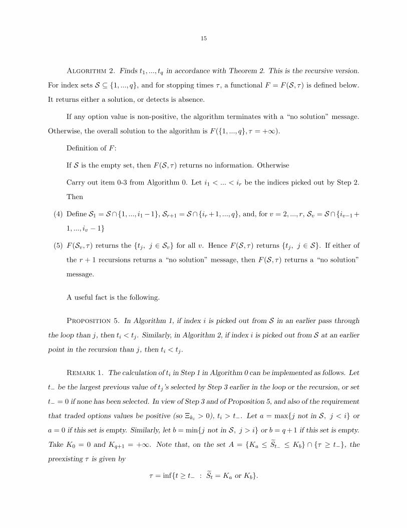
Algorithm 2. Finds t1, ..., tq in accordance with Theorem 2. This is the recursive version.
For index sets S ⊆ 1, ..., q, and for stopping times τ , a functional F = F (S, τ) is defined below.
It returns either a solution, or detects is absence.
If any option value is non-positive, the algorithm terminates with a “no solution” message.
Otherwise, the overall solution to the algorithm is F (1, ..., q, τ = +∞).
Definition of F :
If S is the empty set, then F (S, τ) returns no information. Otherwise
Carry out item 0-3 from Algorithm 0. Let i1 < ... < ir be the indices picked out by Step 2.
Then
(4) Define S1 = S ∩1, ..., i1 −1, Sr+1 = S ∩ir +1, ..., q, and, for v = 2, ..., r, Sv = S ∩iv−1 +
1, ..., iv − 1
(5) F (Sv, τ) returns the tj, j ∈ Sv for all v. Hence F (S, τ) returns tj, j ∈ S. If either of
the r + 1 recursions returns a “no solution” message, then F (S, τ) returns a “no solution”
message.
A useful fact is the following.
Proposition 5. In Algorithm 1, if index i is picked out from S in an earlier pass through
the loop than j, then ti < tj. Similarly, in Algorithm 2, if index i is picked out from S at an earlier
point in the recursion than j, then ti < tj.
Remark 1. The calculation of ti in Step 1 in Algorithm 0 can be implemented as follows. Let
t− be the largest previous value of tj ’s selected by Step 3 earlier in the loop or the recursion, or set
t− = 0 if none has been selected. In view of Step 3 and of Proposition 5, and also of the requirement
that traded options values be positive (so Ξki> 0), ti > t−. Let a = maxj not in S, j < i or
a = 0 if this set is empty. Similarly, let b = minj not in S, j > i or b = q +1 if this set is empty.
Take K0 = 0 and Kq+1 = +∞. Note that, on the set A = Ka ≤ St− ≤ Kb ∩ τ ≥ t−, the
preexisting τ is given by
τ = inft ≥ t− : St = Ka or Kb.
16
It follows that ti is given by by Step 1 via
E(DO(St−, t−, ti)IA) = PKi∗0 − E(Ki − Sτ )
+IAc (6.1)
where, for Ka ≤ s ≤ Kb,
DO(s, t−, t) = E[(Ki − Sτ∧t)+|St− = s]
is the value at t− of the double barrier put option with starting value s and cumulative volatility
t − t− (from t− onward). Since this function is known to be continuous and strictly increasing in
the volatility, it follows that (6.1) has a unique solution on (t−,+∞) unless the algorithm has been
terminated in Step 0.
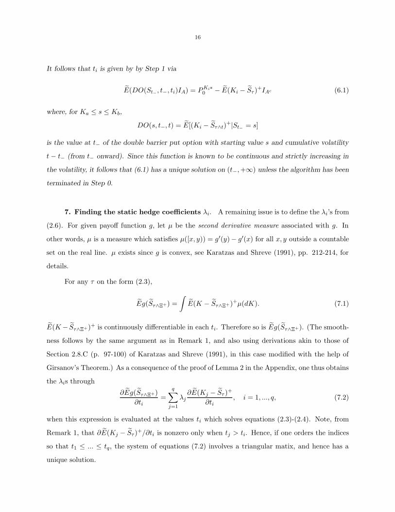
7. Finding the static hedge coefficients λi. A remaining issue is to define the λi’s from
(2.6). For given payoff function g, let µ be the second derivative measure associated with g. In
other words, µ is a measure which satisfies µ([x, y)) = g′(y)− g′(x) for all x, y outside a countable
set on the real line. µ exists since g is convex, see Karatzas and Shreve (1991), pp. 212-214, for
details.
For any τ on the form (2.3),
Eg(Sτ∧Ξ+) =
∫E(K − Sτ∧Ξ+)+µ(dK). (7.1)
E(K− Sτ∧Ξ+)+ is continuously differentiable in each ti. Therefore so is Eg(Sτ∧Ξ+). (The smooth-
ness follows by the same argument as in Remark 1, and also using derivations akin to those of
Section 2.8.C (p. 97-100) of Karatzas and Shreve (1991), in this case modified with the help of
Girsanov’s Theorem.) As a consequence of the proof of Lemma 2 in the Appendix, one thus obtains
the λis through
∂Eg(Sτ∧Ξ+)
∂ti=
q∑
j=1
λj∂E(Kj − Sτ )+
∂ti, i = 1, ..., q, (7.2)
when this expression is evaluated at the values ti which solves equations (2.3)-(2.4). Note, from
Remark 1, that ∂E(Kj − Sτ )+/∂ti is nonzero only when tj > ti. Hence, if one orders the indices
so that t1 ≤ ... ≤ tq, the system of equations (7.2) involves a triangular matix, and hence has a
unique solution.
17
8. Other issues.
Formulation in terms of call options. The results can equally well be put in terms of call
options, but one then needs an additional caveat. We use in the proof of Theorem 1 that (Ki−Sτ∧t)+
is a uniformly integrable martingale from max ti onward. For (Sτ∧t − Ki)+ the same statement
is true for i < q, but for i = q it is not: (Sτ∧t − Kq)+ is a martingale, but its limit at t → +∞
is zero. This can be remedied by requiring τ in (2.3) to be bounded by a constant c, which one
can take to be Ξ+, or max ti, or any other number greater than either. Algorithm 1 then uses the
starting value τ = c rather than τ = +∞. The reason we preferred to avoid this formulation is
that it does not make it clear that τ is, in fact, independent of Ξ+. – This problem does not arise
when evaluating the expectation of g(Sτ∧Ξ+), since Ξ+ is an upper bound on the stopping time.
An alternative formulation in terms of calls would be to replace (2.4) by
E(Sτ − Ki)+ = CKi
0 /Λ0,
with the side condition that τ ≤ tq on the set Stq ≥ Kq. This is again somewhat more inelegant
than the formulation with puts, which is why we have stuck with Theorem 1 as it is.
Lower bounds for prices of convex options. There is no corresponding state price distribution.
For a call or put option payoff g(s) with strike price K, the stopping time τ which would minimize
Eg(Sτ ) would concentrate on the set τ = Ξ∗+ or Sτ = K or Sτ = Ki. Thus the distribution
would depend on the strike price. Also, if one also introduces a lower bound on∫ T0 σ2
t dt, this lower
bound can also be effective.
APPENDIX: PROOFS OF RESULTS
A.1. Proofs of results outside Section 5.
Logical sequence of proofs. For ease of reference, the proofs are given in the order of appear-
ance of the results in the main text. The results, however, depend on each other in a different
logical sequence, and should be taken to be proved in the following order. Proposition 5 is proved
from scratch. Then Theorem 2 is proved using Proposition 5, Proposition 1 is a direct corollary
18
to Theorem 2, and Theorem 1 uses Proposition 1. Proposition 3 (proved in the main text) uses
Theorem 1. Proposition 2 uses both Theorem 1 and the development in Theorem 2. Finally,
Lemmas 1-2 are embedded in the proof of Theorem 1.
Proof of Theorem 1.
Exit Λ, followed by bear. As discussed in Section 2.2, we make use of the discounting by Λt
to restate the problem in terms of finding a self financing strategy in S∗ and the P Ki∗. First of
all, the option liability η = g(ST ) can be reexpressed as η = g(S∗T ), since ΛT = 1. Second, by
numeraire invariance (see Duffie (1996), Chapter 6), Vt is a self financing portfolio in the securities
S, Λ and the P Ki if and only if V ∗t = Vt/Λt is a self financing strategy in the forward contracts
given by S∗ and the P Ki∗. Since VT = V ∗T , the liability η will by covered by V if and only if it is
covered by V ∗. – It is enough, therefore, to prove Theorem 1 as if the Λ process were identically
equal to 1. In other words, as if uninvested cash were stored in the matress.
The function g can be taken to be bounded below. Without loss of generality, we can assume
that the g function is bounded below. This is because, by convexity, there is a constant c1 so that
g1(s) = g(s) + c1s is bounded below. One can then hedge the liability g(ST ) by instead hedging
g1(ST ), and in addition take a static position of −c1 units of security S.
Reformulation of the problem. We shall consider related problems on the set Ω′ = C[0, T ],
with coordinate process (S∗t ), and prespecified initial value S∗
0 . We work with various collections
of probabilities.
R∗Ξ+ is the set of probabilities so that S∗ is a martingale satisfying (1.1), in particular,
dS∗t = σtS
∗t dW ∗
t , (A.1)
and so that for given P ∗ ∈ R∗Ξ+ the process (σt) must be bounded with probability one. We also
require P ∗(IΞ+
) = 1 for all P ∗ ∈ R∗Ξ+ . Also,
P∗Ξ+ = P ∗ ∈ R∗
Ξ+ : E∗(Ki − S∗T )+ = PKi∗
0 .
Note that P∗∞ extends to Q∗ on Ω. Define
V 0(g) = supP ∗∈P∗
Ξ+
E∗g(S∗T ). (A.2)
19
and
V0(g;λ) = supP ∗∈R∗
Ξ+
E∗hλ(S∗T ). (A.3)
By the Dambis (1965)/Dubins-Schwartz (1965) time change,
V0(g;λ) = sup0≤τ≤Ξ+
Ehλ(Sτ ), (A.4)
where τ describe all stopping times in the interval [0,Ξ+]. Finally set
V0(g) = infλ
V0(g;λ) (A.5)
First, by a Lagrange argument, we get
Solution of (A.4)-(A.5), and equality to (A.2). Problem (A.4) can be solved using standard
procedure for American options (see Karatzas (1988), Myneni (1992), and the references therein),
which yield that the supremum is attained at a stopping time τ ∗λ . The American option argument
makes use of the Snell envelope for hλ, which reenters the discussion below:
SE(s,Ξ;λ) = supΞ≤τ≤Ξ+
E(hλ(Sτ ) | SΞ = s).
By an argument similar to that of Theorem 3 of Mykland (2003b), τ ∗λ = τλ ∧ Ξ+, where
τλ = inft : t ≥ tλi and Sτ = Ki for some i, 1 ≤ i ≤ q.
Lemma 1. Suppose that g is bounded below with |g(s)| ≤ a + bs2−ε. Also assume that
(2.3)-(2.4) has a solution τ satisfying (2.5), Then there is such a τ so that V0 = Eg(Sτ∧Ξ+).
Proof of Lemma 1. Consider a sequence of λs so that V0(g;λ) converges to V0(g). Since the
tλi s live in the compact set [0,Ξ+]q, there is a subsequence which is convergent in the tλi s. Call the
relevant limit ti, and define τ ∗ as the limit of the τ ∗λ as one passes through the subsequence. By
uniform integrability, and since S is a continuous process, Eg(Sτ∗
λ) → Eg(Sτ∗) and, for i = 1, ..., q,
E(Ki − Sτ∗
λ)+ → E(Ki − Sτ∗)+. Also, τ∗ can be taken to be on the form τ ∧Ξ+, where τ is on the
form (2.3), again since S is a continuous process.
20
τ∗ must satisfy (2.4), otherwise the infimum in (A.5) would not be finite. By the argument
just underneath the statement of Lemma 1, τ ∗ can be replaced by τ for the purpose of satisfying
(2.4).
If (2.3)-(2.5) has a solution, V 0(g) > −∞. This is because, since (Ki − Sτ∧t)+ is a uniformly
integrable martingale from max ti onward, the constraint (2.4) will also be satisfied if τ is replaced
by τ ∧ Ξ+, provided max ti ≤ Ξ+. Hence also V 0(g) ≤ V0(g). Lemma 1 then shows that V 0(g) =
V0(g).
Connection to the worst case distribution, and the trading strategy. Now combine Lemma 1
with Proposition 1 to see that
V 0(g) = V0(g) =
∫g(s)dFΞ+
(s).
Also, observe that V 0(g) must be a lower bound for the starting value V ∗0 of any self financing
strategy (V ∗t ) for which V ∗
T ≥ g(S∗T ) on IΞ+
. This is because any strategy would have to be self
financing and solvent under each P ∗ ∈ P∗Ξ+ , cf. the development in Mykland (2000, 2003a), and
the literature on superhedging cited in the introduction to the former of these two papers, cf. also
Section 2.2 in this paper.
Existence of a self financing strategy with initial value V 0(g) = V0(g). Theorem 1 will have
been shown if V ∗0 can be taken to be V0(g). To do this, observe that
Lemma 2. Under the assumptions of Lemma 1, there is a (finite) value of λ to that V0(g) =
V0(g;λ). This value is the unique solution of the system of equations (7.2).
For this λ, the process V ∗t = SE(S∗
t ,Ξ+ −∫ t0 σ2
udu, λ) satisfies our requirements for a self
financing strategy in S∗ that is solvent on IΞ+
, for all P ∗ ∈ R∗∞, and hence for all P ∈ Q. This is,
again, by the Dambis/Dubins-Schwartz time change, and by the solution for the American payoff
hλ(Sτ ) under the model (2.1).
Proof of Lemma 2. For a given values of λi, the values of ti that minimize V0(g;λ) must
satisfy equations (7.2). Also, by the triangular matrix argument mentioned in Section 7, this
system of equations defines the λi’s from the minimizing ti’s. When one takes the limit in Lemma 1,
21
equation (7.2) therefore remains valid, by continuity of ∂Eg(Sτ∧Ξ+)/∂ti and the ∂E(Kj − Sτ )+/∂ti.
This ends the proof of Theorem 1.
Proof of Proposition 2. If (2.3)-(2.4) has no solution, this means that there will be a pass
though the loop in Algorithm 1 where step 0 returns a no solution message. Let S be the index set
at this stage, and let I ∈ S be an index that causes the termination condition to be triggered. The
arbitrage strategy is then constructed as in the proof of Proposition 3, in view of (A.10) below.
Proof of Proposition 5. We only show the loop case. The recursion case is similar.
Let t− be as in Remark 1. In the first pass through the loop, Step 1 sets ti = ΞKi. This
value will exceed t− = 0.
We now proceed by induction, assuming that we have gone through n passes of the loop,
n ≥ 1. We need to show that all ti found in Step 1 strictly exceed t−.
If ti = t−, then, the index i would have been selected in the previous pass. If ti < t−, this
means that there is a set j1, ..., jr so that the tjkhave already been picked out in earlier passes
through the loop, and so that
ti ≤ tj1 ≤ ... ≤ tjr = t−, (A.6)
where at least one of the inequalities is strict. Let l be the pass of the loop where tj1 is picked out,
and let τ ′ be the τ given by Step (3) in pass number l − 1. (If l = 1, then τ ′ = +∞).
Since (Ki − St)+ is a martingale for t ≥ ti, it follows that
E(Ki − Sτ∧ti)+|Fti) = (Ki − Sτ∧ti)
+ = (Ki − Sτ ′∧ti)+. (A.7)
Hence, by taking unconditional expectations, and using (A.6),
E(Ki − Sτ ′∧ti)+ = PKi∗
0 .
It follows that index i would give rise to value ti in Step 1 of the l’s iteration of the loop.
22
Let Sn be the set of unselected indices at the start of iteration n+1, and set S cn = 1, ..., q−S.
There are two possibilities in (A.6): either, for some k < r,
ti ≤ tj1 = ... = tjk< tjk+1
≤ t−, (A.8)
or there is no such k, in which case
ti < tj1 = ... = tjr = t−. (A.9)
In the event of (A.8), Step 1 of pass l of the loop gives the values tj1 = ... = tjkfor indices
j1, ..., jk. Also, the indices in jk+1, ..., jr ∪ (Scn − i) are rejected in Step 2. Hence, at most,
i, j1, ..., jk are selected in Step 2, and possibly only i. In the event of (A.9), the same reasoning
applies. In any case, index i is picked out in iteration l < n + 1, the current iteration number of
the loop. Hence, again, if ti were strictly smaller than t−, it would already have been picked out
by the loop in a previous step.
Proof of Theorem 2. (a) is trivial. We do the proof of the rest in steps (i)-(iii) below. (c)
follows from (i) and (ii), (d) follows from (i) and (iii), (b) follows from (c) and (d) in the statement
of the theorem.
(i) Algorithm 1, provided there is no termination in Step 0 at any point in the loop, provides
a unique result t1, ..., tq .
This follows from Proposition 5 and Remark 1.
(ii) Assume that Algorithm 1 has a solution t1, ..., tq . Then this solution satisfies (2.3)-(2.4).
To see this, let τ ′ be the τ from Step 3 in the loop where ti was picked out from S. We now
use τ to denote the final product of Algorithm 1. (A.7) will remain valid, and integrating gives
E(Ki − Sτ )+ = PKi∗
0 .
which is what we needed to show.
(iii) Assume that (2.3)-(2.4) has a solution t1, ..., tq . Then this solution coincides with the
output of Algorithm 1.
23
To see this, consider the order statistic t(1) ≤ ... ≤ t(q). Obviously, if t(1) = ti for some i,
then this index i must be picked out in the first passage through the loop of Algorithm 1, and ti
must have the same value as the ti picked out by the Algorithm. (If there are several ti’s with the
same smallest value, the same applies). Similarly, by induction, one assumes that t(1) ≤ .. ≤ t(j)
coincide with the results of Algorithm 1, and it is then easy to see that t(j+1) also coincides with
the results of the Algorithm, in view of Proposition 5. Note that the termination condition in Step
0 cannot be triggered, since with the τ from the previous step,
E(Ki − Sτ∧ti)+ < E(Ki − Sτ )
+. (A.10)
A.2. Proof for Section 5.
Proof of Proposition 4. Consider first the case 1 ≤ i ≤ q − 1. We show the result for the
density f of Yt = log St = Wt − t/2 given log Ki < Yt < log Ki+1. The density of the proposition
follows by a change of variable, and is f(log(s))/s.
Following the discussion in Section 13 (pp. 330-332) of Karlin and Taylor (1981), and in
particular equation (13.11), f(y) = cm(y)φ1(y) + o(1), where c is a normalizing constant, and the
other quantities are as defined by Karlin and Taylor. In particular, m(y) = e−y, while the φn(y)’s
are solutions to the eigenvalue problem Lφn = −λnφn, with φn(log Ki) = φn(log Ki+1) = 0. Here, L
is the infinitesimal generator, in this case Lφ = 12φ′′− 1
2φ′. Obviously, for log(Ki) < y < log(Ki+1),
φn(y) = cne1
2y sin
(nπ
y − log(K1)
log(K2) − log(K1)
)and λn =
1
2
((nπ)2 +
1
8
),
where the cn’s are constants. By requiring f to integrate to 1, one obtains c as given by (5.2) in
the main text.
Meanwhile, for the lower edge, let t > t1 and x < log K1). By Girsanov’s Theorem,
P (Yt ≤ y | Yt1 = x and maxt1<s<t
Ys < log K1) =E exp(−Wu)I(Wu ≤ y − x and Mu ≤ log K1 − x)
E exp(−Wu)I(Mu ≤ log K1 − x)
24
where u = t− t1, W is a standard Brownian motion, and M is the running maximun of W . Thus,
in this case, for y < log K1, and using, say, formula (8.2) (p. 95) in Karatzas and Shreve (1991),
f(y) ∝ u−1/2 exp(−1
2(y − x))
[φ
(y − x
u1/2
)− φ
(y + x − 2 log K1
u1/2
)].
This gives the result of the proposition. The derivation for the upper edge is similar.
Acknowledgments. The author would like to thank Probal Chaudhuri, Steven Lalley and
Lan Zhang for invaluable advice and discussions.
REFERENCES
Avellaneda, M., Levy, A., and Paras, A. (1995). Pricing and hedging derivative securities in
markets with uncertain volatilities, Appl. Math. Finance 2 73-88.
Bergman, Y.Z., Grundy, B.D., and Wiener, Z. (1996). General properties of option prices, J.
Finance 5 1573-1610.
Black, F., and Scholes, M. (1973). The pricing of options and corporate liabilities, J. Polit. Econ.
81 637-654.
Cvitanic, J., and Karatzas, I. (1992). Convex duality in constrained portfolio optimization, Ann.
Appl. Probab. 2 767–818.
Cvitanic, J., and Karatzas, I. (1993). Hedging of contingent claims with constrained portfolios,
Ann. Appl. Probab. 3 652-681.
Dambis, K. (1965). On the decomposition of continuous sub-martingales, Theory Probab. Appl.
10 401–410.
Dubins, L.E., and Schwartz, G. (1965). On continuous martingales, Proc. Nat. Acad. Sci. U.S.A.
53 913–916.
Duffie, D. (1996). Dynamic Asset Pricing Theory (2nd ed.) (Princeton).
Eberlein, E., and Jacod, J. (1997). On the range of options prices, Finance and Stoch. 1 131-140.
El Karoui, N., Jeanblanc-Picque, M., and Shreve, S.E. (1998). Robustness of the Black and Scholes
formula, Math. Finance 8 93-126.
25
El Karoui, N. and Quenez, M.-C. (1995). Dynamic programming and pricing of contingent claims
in an incomplete market, SIAM J. Contr. Opt. 33 29-66.
Frey, R. (2000). Superreplication in stochastic volatility models and optimal stopping, Finance
and Stochastics 4 161-188.
Frey, R. and Sin, C. (1999). Bounds on European options prices under stochastic volatility, Math.
Finance 9 97-116.
Friedman, C. (2000). Confronting model misspecification in finance: Tractable collections of sce-
nario probability measures for robust financial optimization problems (preprint).
Fritelli, M. (2000). Intrduction to a theory of value coherent with the no-arbitrage principle.
Finance and Stochastics 4 275–297.
Follmer, H. and Leukert, P. (1999). Quantile Hedging, Finance Stochast 3 251-273.
Follmer, H. and Leukert, P. (2000). Efficient hedging: Cost versus shortfall risk, Finance and
Stochast 4 117-146.
Harrison, J.M., and Kreps, D.M. (1979). Martingales and arbitrage in multiperiod securities
markets, J. Econ. Theory 20 381-408.
Harrison, J. M., and Pliska, S. R. (1981). Martingales and stochastic integrals in the theory of
continuous trading, Stoc. Proc. Appl. 11 215- 260.
Hull, J.C. (2003). Options, Futures and Other Derivatives (5rd Ed.). (Prentice Hall).
Jacod, J., and Shiryaev, A.N. (2003). Limit Theorems for Stochastic Processes (2nd ed.). Springer-
Verlag, New York
Jacquier, E., Polson, N. and Rossi, P.E. (1994). Bayesian analysis of stochastic volatility models
J. Bus. Econ. Statist. 12 371–389.
Karatzas, I. (1988). On the pricing of American options, Appl. Math. Optim. 17 37-60.
Karatzas, I. (1996). Lectures on the Mathematics of Finance (CRM monograph series).
Karatzas, I., and Shreve, S.E. (1991). Brownian Motion and Stochastic Calculus (2nd Ed.)
(Springer-Verlag).
26
Karatzas, I., and Kou, S.G. (1996). On the pricing of contingent claims under constraints, Ann.
Appl. Probab. 6 321–369.
Karlin, S., and Taylor, H.M. (1981). A Second Course in Stochastic Processes (Academic Press,
New York).
Kramkov, D.O. (1996). Optional decompositions of supermartingales and hedging in incomplete
security markets. Probab. Theory Relat. Fields. 105 459-479.
Lyons, T.J. (1995). Uncertain volatility and the risk-free synthesis of derivatives. Appl. Math.
Finance 2 117–133.
Merton, R.C. (1973). Theory of rational options pricing, Bell J. Econ. and Measurement Sci. 4
(Spring) 141-183.
Mykland, P.A. (2000). Conservative delta hedging Ann. Appl. Probab. 10 664–683.
Mykland, P.A. (2003a). Financial options and statistical prediction intervals, Ann. Statist. 31
1413-1438.
Mykland, P.A. (2003b). The interpolation of options, Finance and Stochastics 7 417-432.
Myneni, R. (1992). The pricing of the American option, Ann. Appl. Probab. 2 1-23.


![Hp inc[553]](https://img.pdfslide.us/doc/110x75/58cef4ee1a28abab738b4c8b/hp-inc553.jpg)