Technical Report MeteoSwiss No. 270 Exploring quantile ... · that reflect the spatial and temporal scale of the underlying observations. The local daily product of the CH2011 scenarios

Technical Report MeteoSwiss No. 270

Exploring quantile mapping as a tool to produce

user-tailored climate scenarios for Switzerland

Feigenwinter I., Kotlarski S., Casanueva A., Fischer A.M., Schwierz C., Liniger M. A.

MeteoSwiss

Operation Center 1

CH-8044 Zürich-Flughafen

T +41 58 460 99 99

www.meteoschweiz.ch

ISSN: 2296-0058




Feigenwinter I., Kotlarski S., Casanueva A., Fischer A.M., Schwierz C., Liniger M. A.

Recommended citation:

Feigenwinter I, Kotlarski S, Casanueva A, Fischer AM, Schwierz C, Liniger MA, 2018: Exploring quantile mapping as a tool to produce user-tailored climate scenarios for Switzerland, Technical Re-port MeteoSwiss, 270, 44 pp.

Editor:

Federal Office of Meteorology and Climatology, MeteoSwiss, © 2018

V




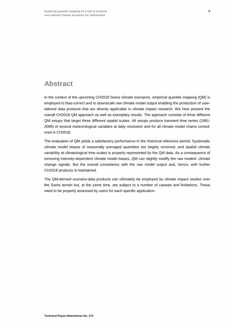
Abstract

In the context of the upcoming CH2018 Swiss climate scenarios, empirical quantile mapping (QM) is

employed to bias-correct and to downscale raw climate model output enabling the production of user-

tailored data products that are directly applicable in climate impact research. We here present the

overall CH2018 QM approach as well as exemplary results. The approach consists of three different

QM setups that target three different spatial scales. All setups produce transient time series (1981-

2099) of several meteorological variables at daily resolution and for all climate model chains consid-

ered in CH2018.

The evaluation of QM yields a satisfactory performance in the historical reference period. Systematic

climate model biases of seasonally averaged quantities are largely removed, and spatial climate

variability at climatological time scales is properly represented by the QM data. As a consequence of

removing intensity-dependent climate model biases, QM can slightly modify the raw models’ climate

change signals. But the overall consistency with the raw model output and, hence, with further

CH2018 products is maintained.

The QM-derived scenario-data products can ultimately be employed by climate impact studies over

the Swiss terrain but, at the same time, are subject to a number of caveats and limitations. These

need to be properly assessed by users for each specific application.

VI


Zusammenfassung Riassunto Résumé

Die neueste Generation Schweizer Klimaszenarien CH2018 verwendet eine empirisch-statistische

Methode, um grob aufgelöste und fehlerbehaftete Klimamodelldaten zu korrigieren und auf lokale

Skalen anzupassen: Quantile Mapping (QM). Die resultierenden QM-basierten Szenario-Produkte

sind damit direkt in einer Vielzahl von Klimafolgenstudien anwendbar. Der vorliegende Bericht gibt

einen Überblick über die in CH2018 verwendete QM Implementation und präsentiert beispielhaft

Ergebnisse. Die Implementation besteht aus drei verschiedenen QM Varianten, die unterschiedliche

räumliche Skalen anvisieren. Alle Varianten liefern transiente Zeitreihen (1981-2099) mehrerer me-

teorologischer Variablen in täglicher Auflösung und für alle in CH2018 verwendeten Klimamodellket-

ten.

Die Validierung des verwendeten QM Ansatzes in einer historischen Referenzperiode zeigt eine

effektive und zufriedenstellende Korrektur systematischer mittlerer Modellfehler. Auch die räumliche

Klimavariabilität wird durch die QM-basierten Produkte gut abgebildet. Zukünftige Klimaänderungs-

signale der rohen, unprozessierten Klimamodelldaten können durch Anwendung von QM zu einem

gewissen Grad verändert werden. Dies beruht in erster Linie auf der erwünschten Berücksichtigung

intensitätsabhängiger Modellfehler durch QM. Prinzipiell wird aber eine Konsistenz mit den Ände-

rungssignalen der rohen Klimamodelldaten und damit auch mit weiteren CH2018 Produkten bewahrt.

Die QM-basierten Szenario-Produkte sind direkt in Klimafolgenstudien in der Schweiz anwendbar. Es

sind bei der Anwendung jedoch auch eine Reihe von Limitierungen und nicht zulässiger Analysen zu

beachten. Diese müssen von Nutzern vor der Verwendung der QM Daten eingeschätzt und entspre-

chend berücksichtigt werden.

VII




Contents

Abstract V

Zusammenfassung Riassunto Résumé VI

1 Introduction 8

2 Data and Methods 10

2.1 Quantile Mapping 10

2.2 Implementation at MeteoSwiss 11

2.3 Climate model data 13

2.4 QM to stations (Setup A) 14

2.5 QM on RCM grid (Setup B) 15

2.6 QM to high-resolution grid (Setup C) 16

2.7 Multi-model combination and pattern scaling 16

2.8 Calculation of temperature indices 17

3 Results 18

3.1 QM evaluation: Individual models 18

3.1.1 QM to stations (Setup A) 18

3.1.2 QM on RCM grid (Setup B) 21

3.1.3 QM to high-resolution grid (Setup C) 23

3.2 QM evaluation: Model ensemble 26

3.3 QM scenarios 29

4 Limitations 36

5 Summary and Conclusions 39

Acknowledgment 40

References 40

VIII


1 Introduction

Climate model data are nowadays used in various fields of application, including the assessment of

future climate change impacts at local to regional scales. Such efforts often require a higher spatial

resolution than currently provided by global or regional climate models (GCMs, RCMs). Furthermore,

climate model data can be subject to systematic biases (e.g. Kotlarski, et al. 2014), which often pre-

vents the direct use of raw climate model output in subsequent applications.

As a response to these challenges and in order to translate coarsely resolved and potentially biased

climate model output into forcing data that are directly applicable to impact models, a large number of

statistical downscaling (SD) and bias correction (BC) approaches have been developed over the

recent decades. Comprehensive overviews are provided by e.g. Wilby and Wigley (2000), Fowler et

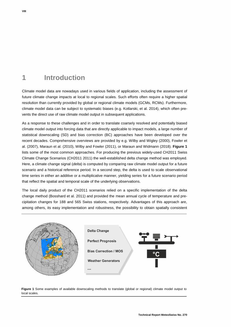
al. (2007), Maraun et al. (2010), Wilby and Fowler (2011), or Maraun and Widmann (2018). Figure 1

lists some of the most common approaches. For producing the previous widely-used CH2011 Swiss

Climate Change Scenarios (CH2011 2011) the well-established delta change method was employed.

Here, a climate change signal (delta) is computed by comparing raw climate model output for a future

scenario and a historical reference period. In a second step, the delta is used to scale observational

time series in either an additive or a multiplicative manner, yielding series for a future scenario period

that reflect the spatial and temporal scale of the underlying observations.

The local daily product of the CH2011 scenarios relied on a specific implementation of the delta

change method (Bosshard et al. 2011) and provided the mean annual cycle of temperature and pre-

cipitation changes for 188 and 565 Swiss stations, respectively. Advantages of this approach are,

among others, its easy implementation and robustness, the possibility to obtain spatially consistent

Figure 1 Some examples of available downscaling methods to translate (global or regional) climate model output to

local scales.

9




multi-site scenario series (based on the observed record at multiple sites) and its inter-variable con-

sistency (based on the observational record of several variables at a given site). However, delta

change is subject to a number of assumptions and limitations. The mean climate change signal is

assumed to be valid for all distributional quantiles (i.e. to apply for both mean and extreme condi-

tions), and systematic model biases are implicitly assumed to be stationary in the long term (i.e. to

apply for both the historical reference and the future scenario period). Furthermore, the temporal

variability of the constructed future time series reflects the variability of the observational period and

potential future changes in temporal climate variability are neglected. Last but not least, delta change

is by definition a time slice-based approach and does not provide information for times between the

end of the reference and the start of the scenario period. Such transient information would have to be

produced by further gap-filling methods.

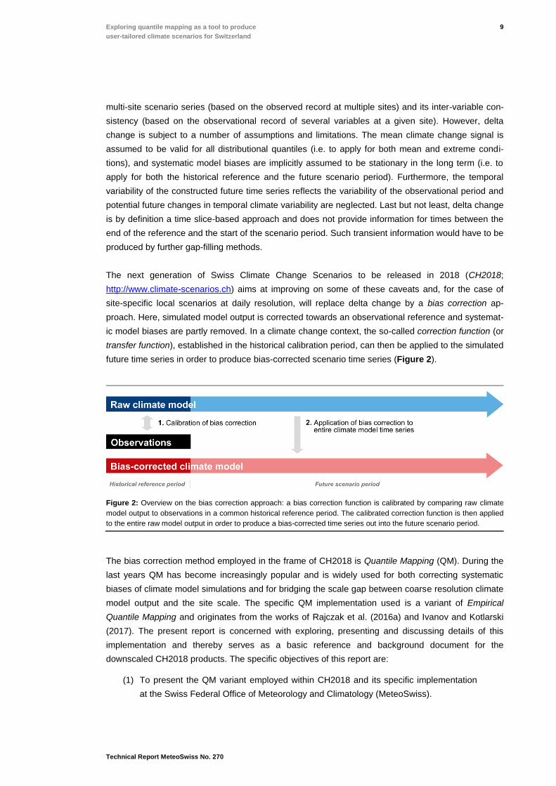
The next generation of Swiss Climate Change Scenarios to be released in 2018 (CH2018;

http://www.climate-scenarios.ch) aims at improving on some of these caveats and, for the case of

site-specific local scenarios at daily resolution, will replace delta change by a bias correction ap-

proach. Here, simulated model output is corrected towards an observational reference and systemat-

ic model biases are partly removed. In a climate change context, the so-called correction function (or

transfer function), established in the historical calibration period, can then be applied to the simulated

future time series in order to produce bias-corrected scenario time series (Figure 2).

Figure 2: Overview on the bias correction approach: a bias correction function is calibrated by comparing raw climate

model output to observations in a common historical reference period. The calibrated correction function is then applied

to the entire raw model output in order to produce a bias-corrected time series out into the future scenario period.

The bias correction method employed in the frame of CH2018 is Quantile Mapping (QM). During the

last years QM has become increasingly popular and is widely used for both correcting systematic

biases of climate model simulations and for bridging the scale gap between coarse resolution climate

model output and the site scale. The specific QM implementation used is a variant of Empirical

Quantile Mapping and originates from the works of Rajczak et al. (2016a) and Ivanov and Kotlarski

(2017). The present report is concerned with exploring, presenting and discussing details of this

implementation and thereby serves as a basic reference and background document for the

downscaled CH2018 products. The specific objectives of this report are:

(1) To present the QM variant employed within CH2018 and its specific implementation

at the Swiss Federal Office of Meteorology and Climatology (MeteoSwiss).

http://www.climate-scenarios.ch/

X


(2) To evaluate the performance of the QM implementation in the historical reference

climate.

(3) To present an exemplary overview of the results obtained in terms of future climate

change over Switzerland as represented by the QM-based scenario products.

(4) To outline potential caveats and limitations of the QM-based products that need to be

taken into account by users.

2 Data and Methods

2.1 Quantile Mapping

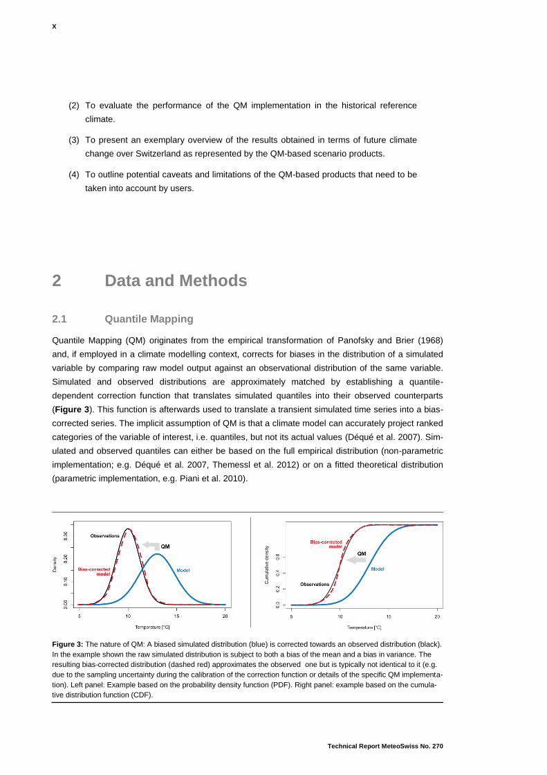
Quantile Mapping (QM) originates from the empirical transformation of Panofsky and Brier (1968)

and, if employed in a climate modelling context, corrects for biases in the distribution of a simulated

variable by comparing raw model output against an observational distribution of the same variable.

Simulated and observed distributions are approximately matched by establishing a quantile-

dependent correction function that translates simulated quantiles into their observed counterparts

(Figure 3). This function is afterwards used to translate a transient simulated time series into a bias-

corrected series. The implicit assumption of QM is that a climate model can accurately project ranked

categories of the variable of interest, i.e. quantiles, but not its actual values (Déqué et al. 2007). Sim-

ulated and observed quantiles can either be based on the full empirical distribution (non-parametric

implementation; e.g. Déqué et al. 2007, Themessl et al. 2012) or on a fitted theoretical distribution

(parametric implementation, e.g. Piani et al. 2010).

Figure 3: The nature of QM: A biased simulated distribution (blue) is corrected towards an observed distribution (black).

In the example shown the raw simulated distribution is subject to both a bias of the mean and a bias in variance. The

resulting bias-corrected distribution (dashed red) approximates the observed one but is typically not identical to it (e.g.

due to the sampling uncertainty during the calibration of the correction function or details of the specific QM implementa-

tion). Left panel: Example based on the probability density function (PDF). Right panel: example based on the cumula-

tive distribution function (CDF).

11




QM as such is a bias correction method but can implicitly include a downscaling component. If the

observed reference data against which the simulated distribution is matched reflects a higher spatial

scale than the underlying climate model data the bias-corrected distribution is, in principle, valid for

that higher spatial scale. A typical example is the mapping of a simulated grid-cell based distribution

(reflecting an area average over the respective climate model grid cell) onto a distribution measured

at a specific weather station. Note, however, that certain aspects of the bias-corrected time series

might still reflect the spatial scale of the underlying climate model. As such, the additional downscal-

ing component involves specific assumptions and comes along with potential risks and limitations

(Maraun 2013, Maraun 2016, Maraun et al. 2017).

A large number of recent studies applied QM in a downscaling context and documented the method’s

general applicability and performance, which is often similar or superior to other statistical downscal-

ing approaches (Boé et al. 2007, Themessl et al. 2011; Gudmundsson et al. 2012; Themessl et al.

2012, Gutiérrez et al. 2018). For the case of Switzerland Rajczak et al. (2016a), Rajczak et al.

(2016b) and Ivanov and Kotlarski (2017) applied and extensively validated QM for a large number of

MeteoSwiss stations and for several meteorological variables that are also targeted in the context of

CH2018.

2.2 Implementation at MeteoSwiss

The QM variant employed in the context of CH2018 is based on the work of Rajczak et al. (2016a),

Rajczak et al. (2016b) and Ivanov and Kotlarski (2017; method linear_add) and has been implement-

ed in the R Software Environment for Statistical Computing and Graphics (https://www.r-project.org).

The Climate Data Operators (CDOs; https://code.mpimet.mpg.de/projects/cdo) were used for further

processing and analysis steps. Most parts of the QM code were run on the Piz Kesch supercomputer

at the Swiss National Supercomputing Centre CSCS. The same QM variant has recently also been

used in a CH2011 extension that provides bias-corrected scenarios for stations that are consistent

with the delta change-based CH2011 products in terms of the underlying climate model chains

Kotlarski et al. (2017). Furthermore, an almost identical methodology has also been applied in a

similar QM implementation to long-range weather forecasts over the Alps. The validation based on a

large sample of 20 years of forecasts showed a good performance in bias removal also in this appli-

cation (Monhart et al., 2018).

The QM implementation is based on the 99 empirical percentiles (1st to 99

th percentile) of the daily

time series and an additive quantile-based correction function that translates simulated quantiles into

their observed counterparts. The correction function in-between the 99 empirical percentiles is linear-

ly interpolated. Values beyond the 1st and the 99

th percentile, and in particular new extremes in the

scenario time series, are corrected according to the correction function of the 1st and 99

th percentile,

respectively. In order to account for seasonally varying bias characteristics the correction function

itself is determined separately for each day-of-the-year (DOY) with a moving 91-day window. For the

case of precipitation, a wet-day threshold of 0.1 mm/day is considered and an additional frequency

adaptation is implemented (e.g. Themessl et al. 2012). This procedure is necessary in the (few) cas-

es where, for a given DOY, the simulated wet-day frequency is smaller than the observed one and

additional wet days have to be included in the corrected series in order to match simulated and ob-

XII


served wet-day frequencies. The dry days in the original model output that need to be replaced by

wet days are chosen by a random number generator. The same is true for the precipitation amount

on these newly introduced wet days, which is randomly drawn from the observed wet day distribu-

tion. For cases where the simulated wet-day frequency is larger than the observed one, QM implicitly

corrects a biased wet day frequency and no separate frequency adaptation is required.

The calibration period of the correction function is 1981–2010 (except for the QM on RCM grid setup

which uses 1981-2008; see below). All simulated quantiles, including those of the future scenario

time series, are estimated applying the correction function calibrated in this period. The resulting

bias-corrected time series is a transient daily series for the entire simulated period 1981–2099 (see

Figure 2).

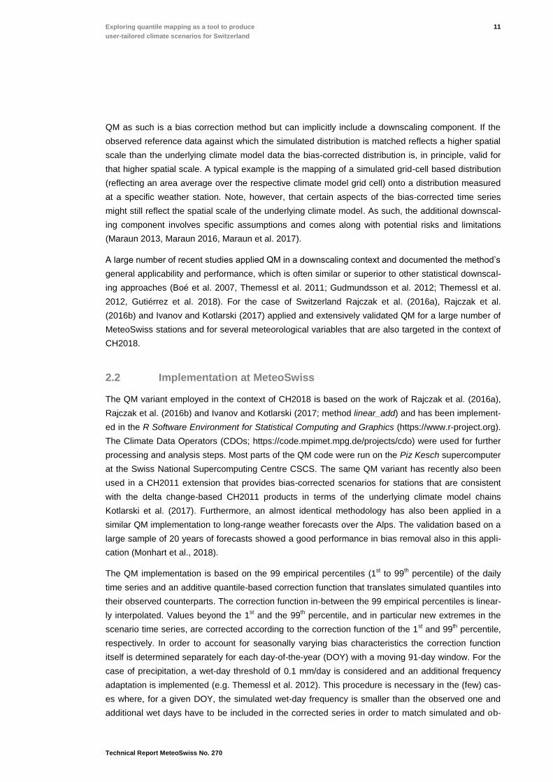
Within CH2018, QM is applied to three different target scales: (A) To the station scale, (B) on the

RCM grid, and (C) to high-resolution 2 km grid covering the Swiss domain. Table 1 gives an over-

view on these different setups and the data involved. Further details are provided in Sections 2.4 to

2.6. Setup A uses station time series as observational reference, while setups B and C employ grid-

ded products derived from observations. Setup B represents a mere bias correction (spatial scale of

the simulations and of the observational reference are identical), while setups A and C additionally

involve a downscaling component (RCM grid to stations and RCM grid to 2km grid, respectively). The

meteorological variables considered depend on the QM setup, but the three temperature variables

(tas, tasmin, tasmax) and precipitation (pr) are covered in all three cases. Setup A (QM to stations) is

the primary product provided to climate scenario users.

Table 1: Overview on the three different QM setups. See Sections 2.4 to 2.6 for further details. Meteorological variables

for which QM is carried out are: daily mean temperature (tas), daily minimum temperature (tasmin), daily maximum

temperature (tasmax), daily precipitation sum (pr), daily mean wind speed (sfcWind), daily mean relative humidity (hurs)

and daily mean global radiation (rsds). The CH2018 domain refers to the combined domain of all five CH2018 regions

(see CH2018 Technical Report).

QM

setup

Observational

data

Model

data

Calibration

period

QM

period Variables

A QM to stations MeteoSwiss daily

station time series

Raw RCM data for

grid cell that is

overlying the sta-

tion location

1981-

2010

1981-

2099

tas, tasmin,

tasmax, pr,

sfcWind,

hurs, rsds

B QM on RCM

grid

MeteoSwiss daily

2 km (TabsD, TminD,

TmaxD, RhiresD) and

further observational

grids regridded to

RCM resolution over

the CH2018 domain

Raw RCM data

(all grid cells of

CH2018 domain)

1981-

2008

1981-

2099

tas, tasmin,

tasmax, pr

C

QM to

high-resolution

grid

MeteoSwiss daily

2 km observational

grids (TabsD, TminD,

TmaxD, RhiresD)

RCM data interpo-

lated to 2 km

resolution

1981-

2010

1981-

2099

tas, tasmin,

tasmax, pr

13




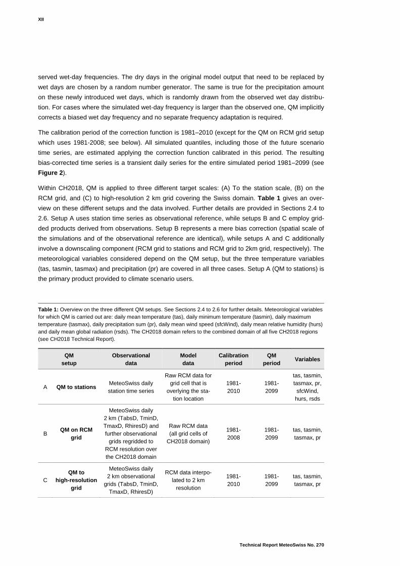
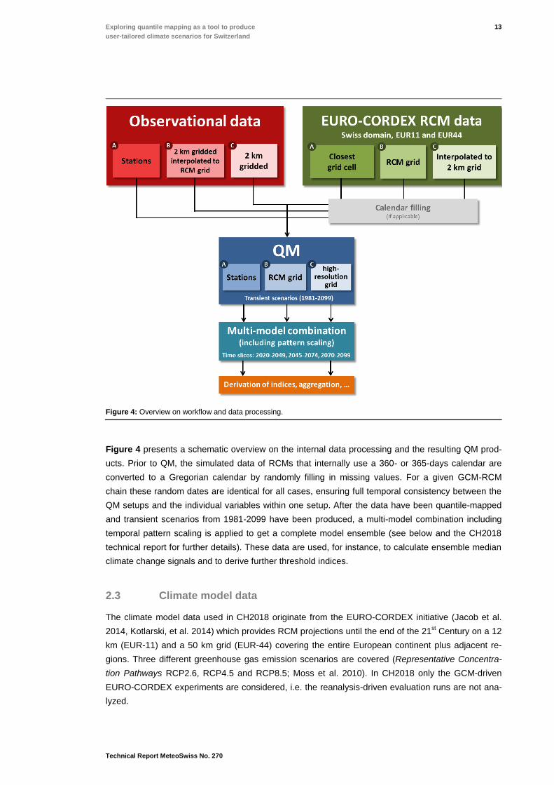
Figure 4: Overview on workflow and data processing.

Figure 4 presents a schematic overview on the internal data processing and the resulting QM prod-

ucts. Prior to QM, the simulated data of RCMs that internally use a 360- or 365-days calendar are

converted to a Gregorian calendar by randomly filling in missing values. For a given GCM-RCM

chain these random dates are identical for all cases, ensuring full temporal consistency between the

QM setups and the individual variables within one setup. After the data have been quantile-mapped

and transient scenarios from 1981-2099 have been produced, a multi-model combination including

temporal pattern scaling is applied to get a complete model ensemble (see below and the CH2018

technical report for further details). These data are used, for instance, to calculate ensemble median

climate change signals and to derive further threshold indices.

2.3 Climate model data

The climate model data used in CH2018 originate from the EURO-CORDEX initiative (Jacob et al.

2014, Kotlarski, et al. 2014) which provides RCM projections until the end of the 21st Century on a 12

km (EUR-11) and a 50 km grid (EUR-44) covering the entire European continent plus adjacent re-

gions. Three different greenhouse gas emission scenarios are covered (Representative Concentra-

tion Pathways RCP2.6, RCP4.5 and RCP8.5; Moss et al. 2010). In CH2018 only the GCM-driven

EURO-CORDEX experiments are considered, i.e. the reanalysis-driven evaluation runs are not ana-

lyzed.

XIV


For the present report all simulations of the CH2018 model freeze 2.0 have been used. This is not

necessarily the final set of model simulations considered in CH2018 as updates of the RCM ensem-

ble might be introduced at a later stage. Freeze 2.0 includes the GCM-driven EURO-CORDEX ex-

periments available in summer 2017 with the exception of a few individual simulations that are disre-

garded due to substantial simulation shortcomings. Furthermore, data for several individual RCMs

have been spatially filtered due to apparent shortcomings in the simulated spatial climate variability.

See the CH2018 freeze 2.0 documentation available on http://www.ch2018.ch/wp-

content/uploads/2017/07/CH2018_model_ensemble.pdf for further details. The total number of simu-

lations considered (summed up over all RCPs) is 81. These experiments were carried out by 26 dif-

ferent GCM-RCM model chains that combine 10 driving GCMs with 10 different RCMs. Note that, as

some experiments do not provide data for all variables, the finally available number of simulations

depends on the specific variable considered. While for daily mean temperature and precipitation all

81 experiments are available, the set for further auxiliary variables is smaller and, for the most ex-

treme case of relative humidity, covers 57 simulations only.

Before applying QM, all raw simulation data have been post-processed and brought to a common

form consisting of daily fields from 1971 to 2099 on one of the standard grids (EUR-11 or EUR-44).

Data of RCMs that internally use a 360- or 365-days calendar were converted to a Gregorian calen-

dar by randomly filling in missing values (see above). Several model chains include additional miss-

ing values at a few time steps due to missing raw RCM data at the very beginning or at the end of the

respective control and scenario simulations. Furthermore, as the focus region of CH2018 is Switzer-

land and to increase computational performance, a Swiss mask has been applied to the European-

scale EUR-11 and EUR-44 grids, resulting in reduced grids covering the area of Switzerland plus

neighboring regions only. Depending on the resolution this reduced grid comprises 768 (EUR-11) or

48 (EUR-44) grid cells in total, defined by a 36x24 or 9x6 rectangle, respectively. With respect to the

full EUR-11 (424x412 grid cells) and EUR-44 (106x103 grid cells) domains these rectangles are

located at positions [181:216,169:192] and [46:54,43:48], respectively. The data format of both the

original EURO-CORDEX data and of the post-processed CH2018 versions is the Network Common

Data Form (NetCDF; https://www.unidata.ucar.edu/software/netcdf).

2.4 QM to stations (Setup A)

For QM to the station scale (setup A; see Figure 4) the closest grid cell of the model data provides

the simulated input series. The observational data consists of station-based time series obtained

from the MeteoSwiss Data Warehouse (DWH). Two different station sets are considered:

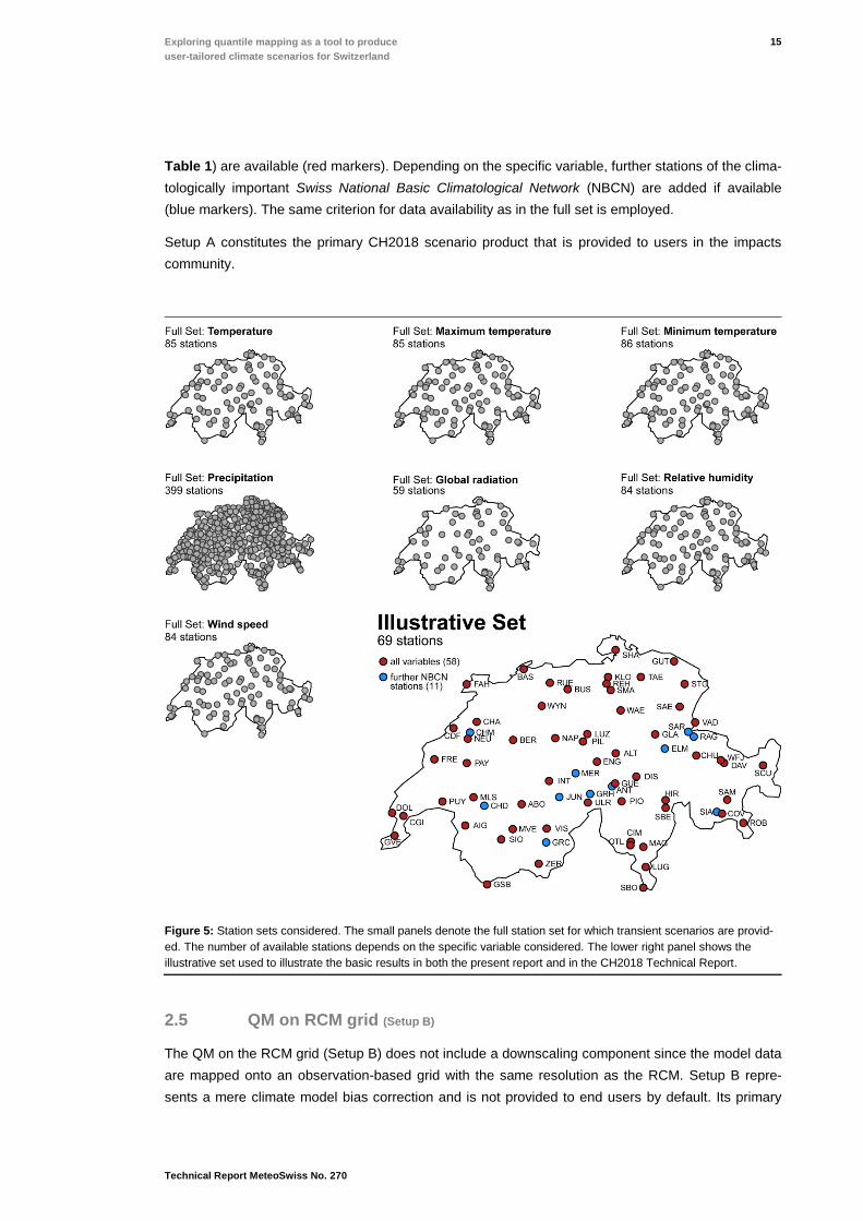
The full set (Figure 5, small panels) covers all stations for which transient QM-based scenarios will

be provided in the context of CH2018. It comprises all Swiss stations for which daily data are availa-

ble during at least 83% of the entire calibration period 1981-2010 (25 out of 30 years) and during at

least 83% of the time for each individual DOY. The number of stations in the full set depends on the

specific meteorological variable considered and varies from 59 (global radiation) to 399 (precipita-

tion).

The illustrative set (Figure 5, lower right panel) is a subset of the full set. It is used to present the

main results of the station-based scenarios in both this report and in the CH2018 Technical Report. It

consists of a basic set of 58 stations at which all seven meteorological variables considered (see

http://www.ch2018.ch/wp-content/uploads/2017/07/CH2018_model_ensemble.pdf

http://www.ch2018.ch/wp-content/uploads/2017/07/CH2018_model_ensemble.pdf

https://www.unidata.ucar.edu/software/netcdf

15




Table 1) are available (red markers). Depending on the specific variable, further stations of the clima-

tologically important Swiss National Basic Climatological Network (NBCN) are added if available

(blue markers). The same criterion for data availability as in the full set is employed.

Setup A constitutes the primary CH2018 scenario product that is provided to users in the impacts

community.

Figure 5: Station sets considered. The small panels denote the full station set for which transient scenarios are provid-

ed. The number of available stations depends on the specific variable considered. The lower right panel shows the

illustrative set used to illustrate the basic results in both the present report and in the CH2018 Technical Report.

2.5 QM on RCM grid (Setup B)

The QM on the RCM grid (Setup B) does not include a downscaling component since the model data

are mapped onto an observation-based grid with the same resolution as the RCM. Setup B repre-

sents a mere climate model bias correction and is not provided to end users by default. Its primary

XVI


purpose is to assess uncertainties of climate change signals at larger spatial scales (CH2018 region-

al domains) and to evaluate potential modifications of the raw climate change signal by QM.

Several gridded observational datasets have been merged to provide the reference observations for

this QM setup. As a large-scale background data reference, the gridded E-OBS dataset (Haylock et

al. 2008) which is available for the whole EURO-CORDEX domain at 25 km resolution is employed.

For constructing a reference on the higher-resolved EUR-11 grid, E-OBS has been spatially re-

mapped (nearest neighbor remapping) from 25 to 12 km. Over the Alps the E-OBS reference is re-

placed by spatially aggregated high-resolution gridded observations (first-order conservative re-

mapping): Over Switzerland the 2 km gridded datasets of MeteoSwiss (TabsD, TminD, TmaxD,

RhiresD) are used; in addition, for precipitation outside of Switzerland the Alpine Precipitation Grid

Dataset (APGD) with 5 km resolution (Isotta, et al., 2014) is employed. For obtaining an observation-

al reference at the coarser EUR-44 resolution, the merged EUR-11 reference grid was spatially ag-

gregated (first-order conservative remapping) from 12 to 50 km resolution.

2.6 QM to high-resolution grid (Setup C)

QM to high-resolution grid (Setup C) again includes a downscaling step in addition to a bias correc-

tion. In contrast to Setup A, QM is applied in a spatially explicit manner yielding complete spatial

grids of downscaled and bias-corrected data which are provided to users on request. Prior to QM the

model data were conservatively remapped from the original RCM grid (EUR-11 or EUR-44) to the 2

km grid of the observational reference using the CDO operator cdo remapcon. As observational ref-

erence the MeteoSwiss 2 km gridded products TabsD, TminD, TmaxD (MeteoSwiss 2016a) and

RhiresD (MeteoSwiss 2016b) were used. Since these data are only available for the area of Switzer-

land, the resulting QM product covers Switzerland only. Note that the spatially continuous application

of QM with a downscaling component is associated with certain caveats (see below and the CH2018

Technical Report), and the 2 km gridded QM product has to be used with special care.

2.7 Multi-model combination and pattern scaling

All QM setups (A, B and C) are carried out for the entire CH2018 freeze 2.0 ensemble. For the

CH2018 ensemble analysis and visualization, the set of available RCM experiments of the model

freeze 2.0 is afterwards recombined into a multi-model combination. This procedure is applied for the

raw experiments and also for the quantile-mapped data (all setups).

First, EUR-44 experiments for which also a EUR-11 version is available (i.e., an experiment carried

out by the same model chain but at higher resolution) are excluded in order to minimize interdepend-

encies. Secondly, in order to provide climate change information for all emission scenarios, a tem-

poral, time slice-based pattern scaling is employed to substitute missing experiments for RCP2.6 or

RCP4.5 for which a corresponding experiment for RCP4.5 or RCP8.5 is available. This method is

based on changes in the global mean temperature (GMT) as simulated by the driving GCMs (Herger,

et al., 2015). For a given scenario period these changes are typically largest in high emission scenar-

ios (e.g., RCP8.5) and the corresponding GMT change for a low emission scenario (e.g., RCP2.6) is

reached in an earlier period. This 30-year period (corresponding to the GMT change in a low emis-

sion scenario) is searched for in the GCM simulation based on the high emission scenario. The cor-

17




responding period in the EURO-CORDEX GCM-RCM chain is used as a substitute in case that no

GCM-RCM experiment is available for the low emission scenario. For missing RCP2.6 experiments

the neighboring scenario RCP4.5 is used if available. If RCP4.5 does not exist, both the RCP2.6 and

RCP4.5 scenario are substituted by pattern-scaling the RCP8.5 run. See the CH2018 Technical

Report for further details. As a result, the number of (real or substituted) simulations is identical for all

RCPs and, depending on the variable, amounts to 15 to 26 (26 simulations for temperature and pre-

cipitation and less for further auxiliary variables).

For a given RCP, the overall rule for choosing/excluding and substituting simulations in the multi-

model combination can be summarized as

EUR-11 simulations > EUR-44 simulations > EUR-11 pattern scaling > EUR-44 pattern scaling

This means that, first, original simulations are preferred over the pattern-scaled substitution. Second,

the higher (EUR-11) resolution is preferred over the lower (EUR-44) resolution.

For derivation of climate change signals in the multi-model combination, three distinct scenario peri-

ods are related to the reference period 1981-2010: 2020-2049, 2045-2074 and 2070-2099. For rea-

sons of simplicity, these periods are denoted by the corresponding central year of the time window

(2035, 2060 and 2085, respectively).

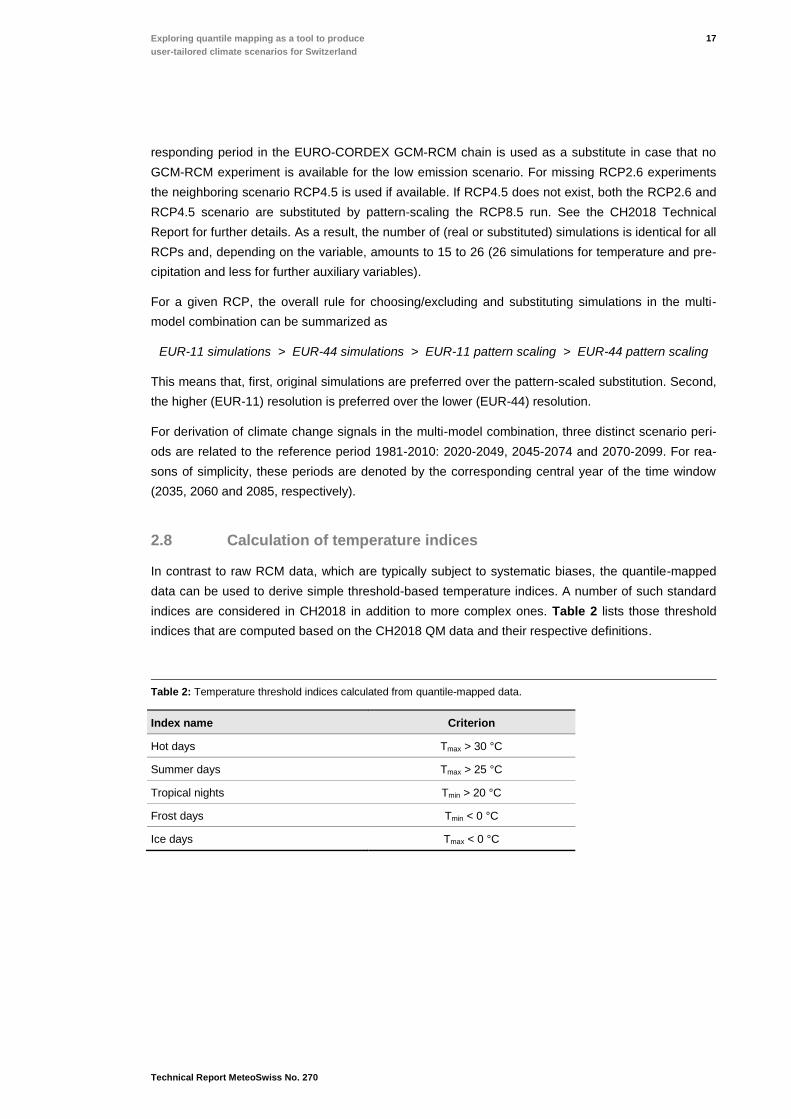
2.8 Calculation of temperature indices

In contrast to raw RCM data, which are typically subject to systematic biases, the quantile-mapped

data can be used to derive simple threshold-based temperature indices. A number of such standard

indices are considered in CH2018 in addition to more complex ones. Table 2 lists those threshold

indices that are computed based on the CH2018 QM data and their respective definitions.

Table 2: Temperature threshold indices calculated from quantile-mapped data.

Index name Criterion

Hot days Tmax > 30 °C

Summer days Tmax > 25 °C

Tropical nights Tmin > 20 °C

Frost days Tmin < 0 °C

Ice days Tmax < 0 °C

XVIII


3 Results

In the following we present exemplary and summary results of the QM application in the context of

CH2018. First, we verify and evaluate the QM implementation. For this purpose the full calibration

period 1981-2010 (or 1981-2008 for Setup B) is considered. This means that evaluation and valida-

tion period are identical and no independent cross-validation exercise is carried out. The latter was

covered by previous works (e.g. (Ivanov and Kotlarski 2017, Gutiérrez et al. 2018) which revealed

that QM, in general, performs well in a historical cross-validation setting with independent calibration

and validation periods. In the present report, we focus on a more technical evaluation of the QM

implementation based on a comparison of the quantile-mapped data and observations within the

calibration period itself in order to identify potential errors or shortcomings of the implementation. For

the evaluation exercise we here mostly focus on one individual exemplary model simulation1, but

also consider ensemble median statistics in some cases. Second, we present exemplary results of

the QM-based climate scenarios focusing on QM to stations (Setup A).

3.1 QM evaluation: Individual models

QM is massively applied in the context of CH2018. A large number of climate model simulations

(each one spanning 119 simulation years from 1981–2099), several hundred stations and/or grid

cells and up to seven meteorological parameters are considered (see above). The output produced

has a size of several terabytes. Although the general performance of QM has been verified in previ-

ous works, problems in individual cases cannot be ruled out. Therefore, a number of control sheets

and control figures have been designed which are automatically produced for each QM application

(i.e., for each quantile-mapped climate model chain, each variable and, for the case of QM setup A,

for each station considered). Below we present examples of this control output, focusing on one

exemplary model simulation only (CLMCOM-CCLM4-MPIESM-EUR11-RCP85).

3.1.1 QM to stations (Setup A)

Figure 6 shows an example for a control sheet of QM setup A (QM to stations) for the case of tem-

perature. The upper panels compare annual cycles and seasonal2 PDFs of observational data, RCM

raw data and quantile-mapped model data. The four lower panels provide details on the QM correc-

tion function (averaging the quantile-based correction function over all DOYs within a given season)

1 CLMCOM-CCLM4-MPIESM-EUR11-RCP85, denoting the RCM CLMcom-CCLM4-8-17 driven by the GCM MPI-M-MPI-ESM-LR at

EUR-11 resolution and for emission scenario RCP8.5

2 DJF: Winter (December–February), MAM: Spring (March–May), JJA: Summer (June–July), SON: Autumn (September–November)

19




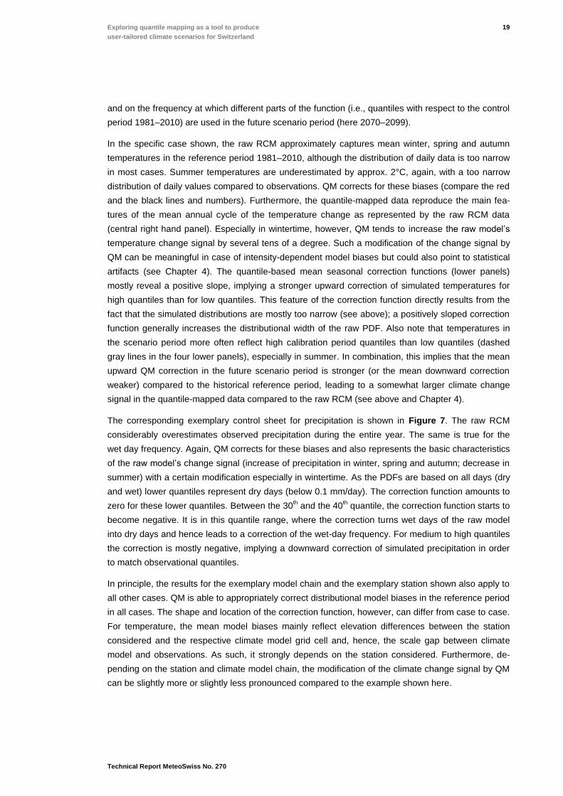
and on the frequency at which different parts of the function (i.e., quantiles with respect to the control

period 1981–2010) are used in the future scenario period (here 2070–2099).

In the specific case shown, the raw RCM approximately captures mean winter, spring and autumn

temperatures in the reference period 1981–2010, although the distribution of daily data is too narrow

in most cases. Summer temperatures are underestimated by approx. 2°C, again, with a too narrow

distribution of daily values compared to observations. QM corrects for these biases (compare the red

and the black lines and numbers). Furthermore, the quantile-mapped data reproduce the main fea-

tures of the mean annual cycle of the temperature change as represented by the raw RCM data

(central right hand panel). Especially in wintertime, however, QM tends to increase the raw model’s

temperature change signal by several tens of a degree. Such a modification of the change signal by

QM can be meaningful in case of intensity-dependent model biases but could also point to statistical

artifacts (see Chapter 4). The quantile-based mean seasonal correction functions (lower panels)

mostly reveal a positive slope, implying a stronger upward correction of simulated temperatures for

high quantiles than for low quantiles. This feature of the correction function directly results from the

fact that the simulated distributions are mostly too narrow (see above); a positively sloped correction

function generally increases the distributional width of the raw PDF. Also note that temperatures in

the scenario period more often reflect high calibration period quantiles than low quantiles (dashed

gray lines in the four lower panels), especially in summer. In combination, this implies that the mean

upward QM correction in the future scenario period is stronger (or the mean downward correction

weaker) compared to the historical reference period, leading to a somewhat larger climate change

signal in the quantile-mapped data compared to the raw RCM (see above and Chapter 4).

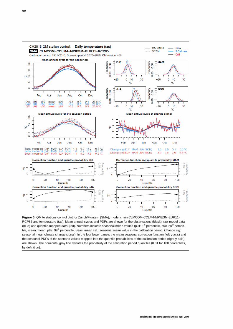
The corresponding exemplary control sheet for precipitation is shown in Figure 7. The raw RCM

considerably overestimates observed precipitation during the entire year. The same is true for the

wet day frequency. Again, QM corrects for these biases and also represents the basic characteristics

of the raw model’s change signal (increase of precipitation in winter, spring and autumn; decrease in

summer) with a certain modification especially in wintertime. As the PDFs are based on all days (dry

and wet) lower quantiles represent dry days (below 0.1 mm/day). The correction function amounts to

zero for these lower quantiles. Between the 30th and the 40

th quantile, the correction function starts to

become negative. It is in this quantile range, where the correction turns wet days of the raw model

into dry days and hence leads to a correction of the wet-day frequency. For medium to high quantiles

the correction is mostly negative, implying a downward correction of simulated precipitation in order

to match observational quantiles.

In principle, the results for the exemplary model chain and the exemplary station shown also apply to

all other cases. QM is able to appropriately correct distributional model biases in the reference period

in all cases. The shape and location of the correction function, however, can differ from case to case.

For temperature, the mean model biases mainly reflect elevation differences between the station

considered and the respective climate model grid cell and, hence, the scale gap between climate

model and observations. As such, it strongly depends on the station considered. Furthermore, de-

pending on the station and climate model chain, the modification of the climate change signal by QM

can be slightly more or slightly less pronounced compared to the example shown here.

XX


Figure 6: QM to stations control plot for Zurich/Fluntern (SMA), model chain CLMCOM-CCLM4-MPIESM-EUR11-

RCP85 and temperature (tas). Mean annual cycles and PDFs are shown for the observations (black), raw model data

(blue) and quantile-mapped data (red). Numbers indicate seasonal mean values (p01: 1st percentile, p50: 50

th percen-

tile, mean: mean, p99: 99th percentile, Seas. mean cal.: seasonal mean value in the calibration period, Change sig:

seasonal mean climate change signal). In the four lower panels the mean seasonal correction function (left y-axis) and

the seasonal PDFs of the scenario values mapped into the quantile probabilities of the calibration period (right y-axis)

are shown. The horizontal gray line denotes the probability of the calibration period quantiles (0.01 for 100 percentiles,

by definition).

21




Figure 7: As Figure 6 but for precipitation and with two adjustments: The upper right panel shows the mean annual

cycle of the wet day frequency in the respective datasets instead of the four seasonal distributions. PDFs of the scenario

period values are omitted in the four lower panels.

3.1.2 QM on RCM grid (Setup B)

In the case of QM on the RCM grid (Setup B), the bias correction has been carried out independently

for each RCM grid cell in the domain. Producing the same control sheets as for Setup A for each grid

cell would result in an unmanageable number of figures. Hence, only summary evaluations in terms

of spatial patterns of seasonal mean values in the observations, in RCM raw output and in quantile-

mapped output are produced operationally. For individual cases, however, detailed evaluations as

shown in Figure 6 and Figure 7 can be produced.

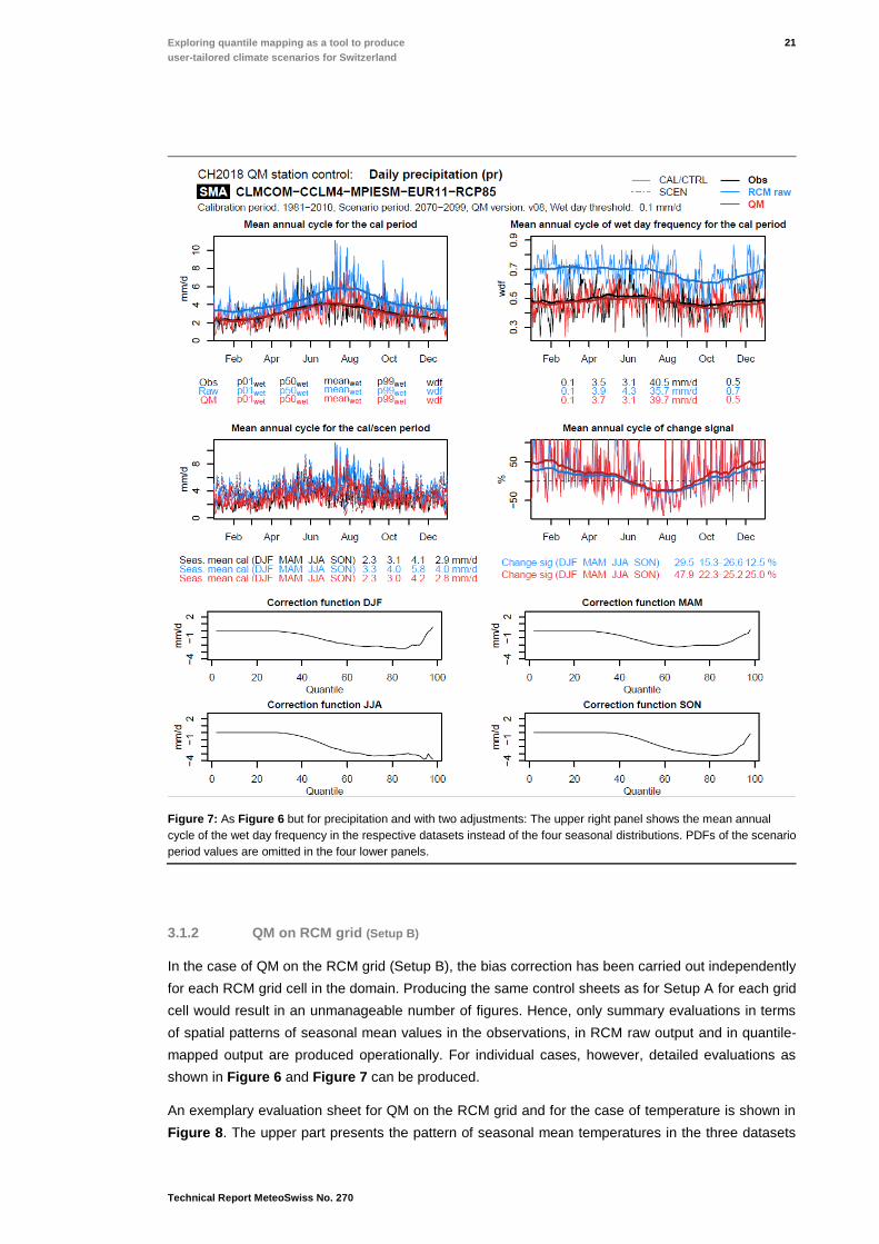
An exemplary evaluation sheet for QM on the RCM grid and for the case of temperature is shown in

Figure 8. The upper part presents the pattern of seasonal mean temperatures in the three datasets

XXII


in the calibration period 1981–2008, the lower part the seasonal mean biases of RCM raw and of

quantile-mapped output when compared against the observational reference. The specific RCM

considered here is subject to a pronounced and widespread cold bias of partly more than 2°C, ex-

cept for the Swiss midlands in winter. After application of QM these biases of seasonal means almost

vanish and are reduced to a few tens of a degree at maximum. Such remaining biases in the calibra-

tion period can be explained by the approximate nature of the QM implementation (use of the 99

empirical percentiles with linear interpolation in-between) which avoids overfitting and by the use of a

91-day moving window for calibration. The latter implies the consideration of days outside the evalu-

ated 3-month season (e.g., considering days in January and March for correcting February days).

Hence, the QM product can only approximate the fixed-period seasonal mean values (see Figure 3).

Figure 8: QM on RCM grid control plot for the model chain CLMCOM-CCLM4-MPIESM-EUR11-RCP85 and tempera-

ture (tas). The upper rows show the spatial distribution of seasonal mean temperature in the QM calibration period

1981-2008 for the reference observations (OBS), the raw RCM data (RCM raw) and the quantile-mapped data (QM).

The two lower rows show the spatial pattern of the seasonal mean bias of raw and of quantile-mapped RCM data.

23




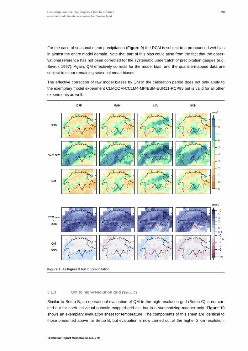
For the case of seasonal mean precipitation (Figure 9) the RCM is subject to a pronounced wet bias

in almost the entire model domain. Note that part of this bias could arise from the fact that the obser-

vational reference has not been corrected for the systematic undercatch of precipitation gauges (e.g.

Sevruk 1997). Again, QM effectively corrects for the model bias, and the quantile-mapped data are

subject to minor remaining seasonal mean biases.

The effective correction of raw model biases by QM in the calibration period does not only apply to

the exemplary model experiment CLMCOM-CCLM4-MPIESM-EUR11-RCP85 but is valid for all other

experiments as well.

Figure 9: As Figure 8 but for precipitation.

3.1.3 QM to high-resolution grid (Setup C)

Similar to Setup B, an operational evaluation of QM to the high-resolution grid (Setup C) is not car-

ried out for each individual quantile-mapped grid cell but in a summarizing manner only. Figure 10

shows an exemplary evaluation sheet for temperature. The components of this sheet are identical to

those presented above for Setup B, but evaluation is now carried out at the higher 2 km resolution.

XXIV


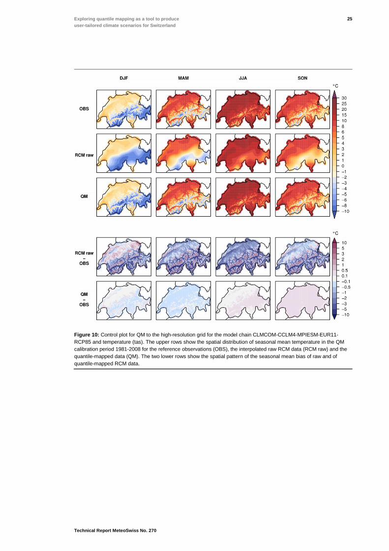
As explained in Chapter 2.6, raw model data were conservatively remapped to this higher spatial

resolution before the application of QM. The corresponding spatial variability of seasonal mean tem-

perature is therefore much lower in the raw RCM output compared to the observational 2 km refer-

ence (compare first and second line in Figure 10). The spatial pattern of the mean biases of RCM

raw (fourth row) is mainly governed by topographic features, reflecting the elevation difference be-

tween the topography of the 2 km grid-resolution of the observational reference and the strongly

smoothed original RCM topography. The predominant bias pattern is characterized by cold biases in

the valleys (RCM grid cell at a higher elevation than 2 km grid cells, implying a systematically lower

temperature) and warm biases aloft (RCM grid cell at a lower elevation, implying a systematically

higher temperature). As expected, QM effectively corrects for these biases and produces spatial

temperature patterns that closely resemble those of the observations. Remaining biases are small

and still subject to a slight topographic control (bottom row in Figure 10).

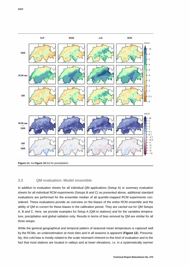
Also for precipitation, spatial variability in the interpolated raw RCM data is much smaller than in the

observational reference (Figure 11). As already apparent from Setup B (see Chapter 3.1.2), the

specific RCM under consideration suffers from a pronounced wet bias in all seasons and over most

parts of the analysis domain. Due to a less pronounced dependence of seasonal precipitation means

on elevation, the spatial bias pattern of raw RCM output is less controlled by topography than in the

case of temperature (fourth row in Figure 11). QM effectively removes the bias of the raw data, and

the resulting quantile-mapped product only shows minor remaining biases (bottom row).

Again, the results presented for the exemplary model experiment CLMCOM-CCLM4-MPIESM-

EUR11-RCP85 with respect to the ability of QM to correct for raw RCM biases in the calibration peri-

od also apply for all other experiments considered in this work.

25




Figure 10: Control plot for QM to the high-resolution grid for the model chain CLMCOM-CCLM4-MPIESM-EUR11-

RCP85 and temperature (tas). The upper rows show the spatial distribution of seasonal mean temperature in the QM

calibration period 1981-2008 for the reference observations (OBS), the interpolated raw RCM data (RCM raw) and the

quantile-mapped data (QM). The two lower rows show the spatial pattern of the seasonal mean bias of raw and of

quantile-mapped RCM data.

XXVI



3.2 QM evaluation: Model ensemble

In addition to evaluation sheets for all individual QM applications (Setup A) or summary evaluation

sheets for all individual RCM experiments (Setups B and C) as presented above, additional standard

evaluations are performed for the ensemble median of all quantile-mapped RCM experiments con-

sidered. These evaluations provide an overview on the biases of the entire RCM ensemble and the

ability of QM to correct for these biases in the calibration period. They are carried out for QM Setups

A, B and C. Here, we provide examples for Setup A (QM to stations) and for the variables tempera-

ture, precipitation and global radiation only. Results in terms of bias removal by QM are similar for all

three setups.

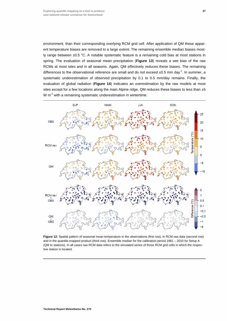
While the general geographical and temporal pattern of seasonal mean temperature is captured well

by the RCMs, an underestimation at most sites and in all seasons is apparent (Figure 12). Presuma-

bly, this cold bias is mostly related to the scale mismatch inherent to this kind of evaluation and to the

fact that most stations are located in valleys and at lower elevations, i.e. in a systematically warmer

27




environment, than their corresponding overlying RCM grid cell. After application of QM these appar-

ent temperature biases are removed to a large extent. The remaining ensemble median biases most-

ly range between ±0.5 °C. A notable systematic feature is a remaining cold bias at most stations in

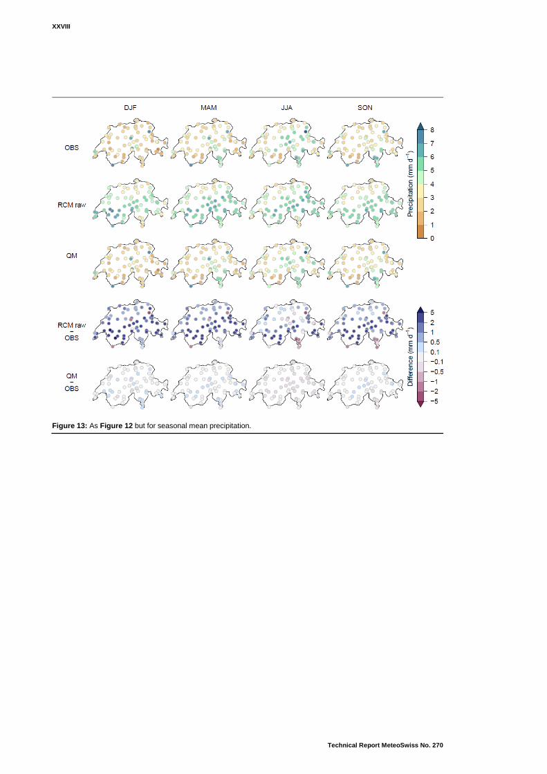
spring. The evaluation of seasonal mean precipitation (Figure 13) reveals a wet bias of the raw

RCMs at most sites and in all seasons. Again, QM effectively reduces these biases. The remaining

differences to the observational reference are small and do not exceed ±0.5 mm day-1

. In summer, a

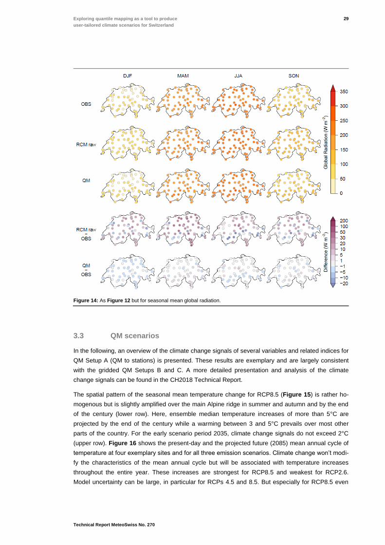
systematic underestimation of observed precipitation by 0.1 to 0.5 mm/day remains. Finally, the

evaluation of global radiation (Figure 14) indicates an overestimation by the raw models at most

sites except for a few locations along the main Alpine ridge. QM reduces these biases to less than ±5

W m-2

with a remaining systematic underestimation in wintertime.

Figure 12: Spatial pattern of seasonal mean temperature in the observations (first row), in RCM raw data (second row)

and in the quantile-mapped product (third row). Ensemble median for the calibration period 1981 – 2010 for Setup A

(QM to stations). In all cases raw RCM data refers to the simulated series of those RCM grid cells in which the respec-

tive station is located.

XXVIII


Figure 13: As Figure 12 but for seasonal mean precipitation.

29




Figure 14: As Figure 12 but for seasonal mean global radiation.

3.3 QM scenarios

In the following, an overview of the climate change signals of several variables and related indices for

QM Setup A (QM to stations) is presented. These results are exemplary and are largely consistent

with the gridded QM Setups B and C. A more detailed presentation and analysis of the climate

change signals can be found in the CH2018 Technical Report.

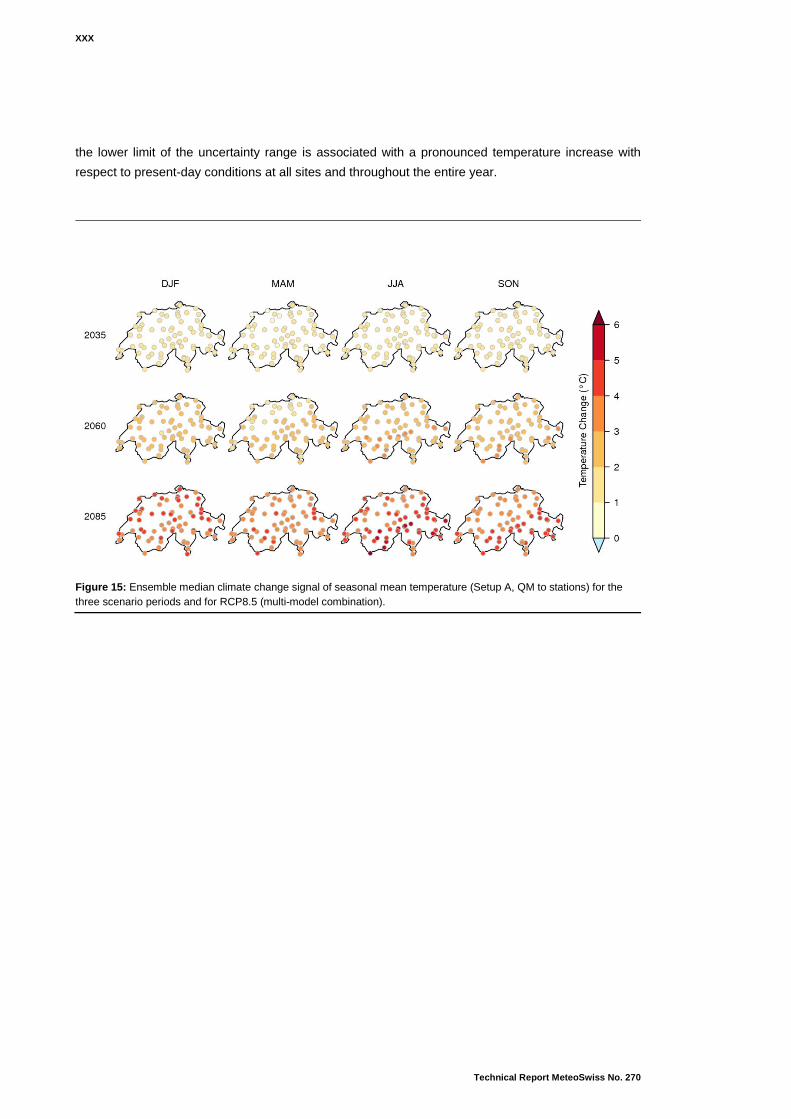
The spatial pattern of the seasonal mean temperature change for RCP8.5 (Figure 15) is rather ho-

mogenous but is slightly amplified over the main Alpine ridge in summer and autumn and by the end

of the century (lower row). Here, ensemble median temperature increases of more than 5°C are

projected by the end of the century while a warming between 3 and 5°C prevails over most other

parts of the country. For the early scenario period 2035, climate change signals do not exceed 2°C

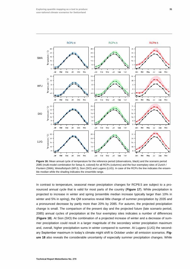
(upper row). Figure 16 shows the present-day and the projected future (2085) mean annual cycle of

temperature at four exemplary sites and for all three emission scenarios. Climate change won’t modi-

fy the characteristics of the mean annual cycle but will be associated with temperature increases

throughout the entire year. These increases are strongest for RCP8.5 and weakest for RCP2.6.

Model uncertainty can be large, in particular for RCPs 4.5 and 8.5. But especially for RCP8.5 even

XXX


the lower limit of the uncertainty range is associated with a pronounced temperature increase with

respect to present-day conditions at all sites and throughout the entire year.

Figure 15: Ensemble median climate change signal of seasonal mean temperature (Setup A, QM to stations) for the

three scenario periods and for RCP8.5 (multi-model combination).

31




Figure 16: Mean annual cycle of temperature for the reference period (observations, black) and the scenario period

2085 (multi-model combination for Setup A, colored) for all RCPs (columns) and the four exemplary sites of Zurich /

Fluntern (SMA), Weissfluhjoch (WFJ), Sion (SIO) and Lugano (LUG). In case of the RCPs the line indicates the ensem-

ble median while the shading indicates the ensemble range.

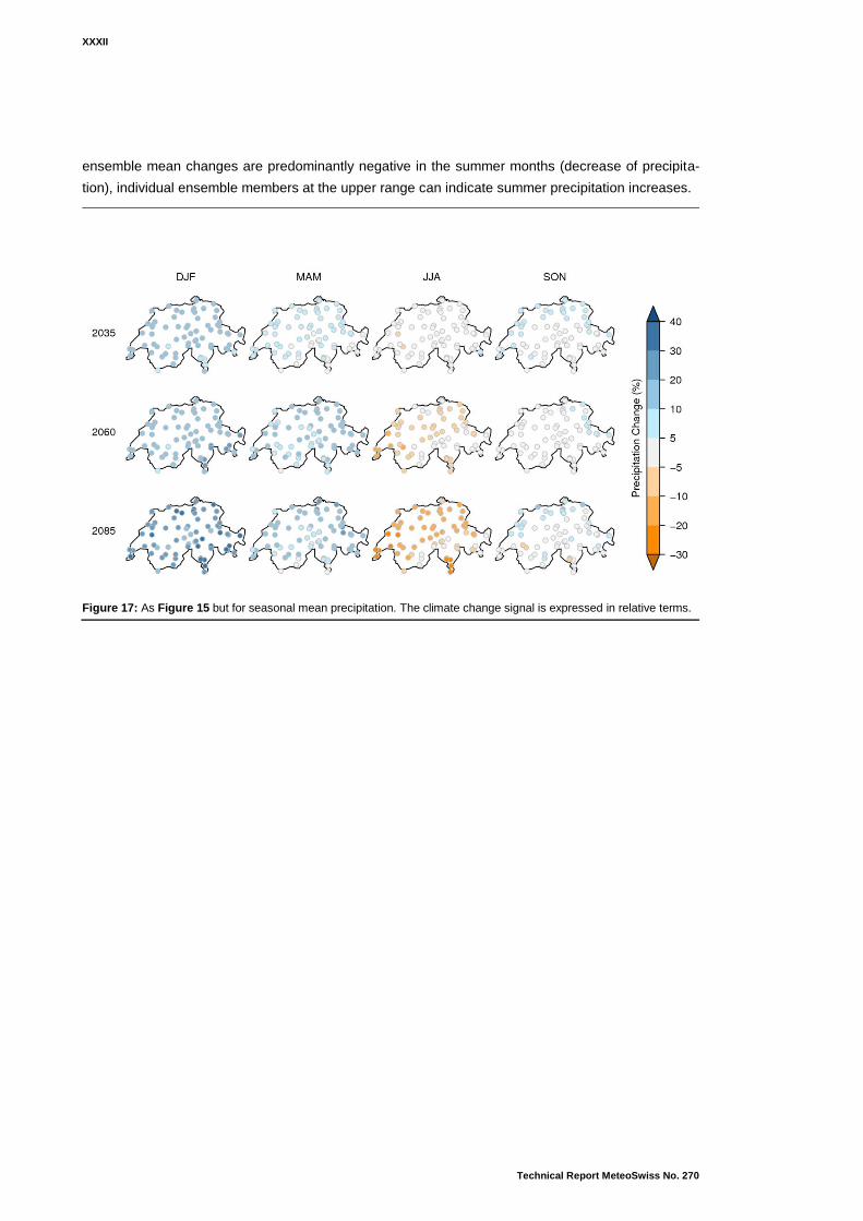
In contrast to temperature, seasonal mean precipitation changes for RCP8.5 are subject to a pro-

nounced annual cycle that is valid for most parts of the country (Figure 17). While precipitation is

projected to increase in winter and spring (ensemble median increase typically larger than 10% in

winter and 5% in spring), the QM scenarios reveal little change of summer precipitation by 2035 and

a pronounced decrease by partly more than 20% by 2085. For autumn, the projected precipitation

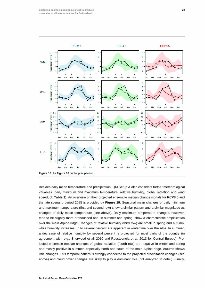
change is small. The comparison of the present day and the projected future (late scenario period,

2085) annual cycles of precipitation at the four exemplary sites indicates a number of differences

(Figure 18). At Sion (SIO) the combination of a projected increase of winter and a decrease of sum-

mer precipitation could result in a larger magnitude of the secondary winter precipitation maximum

and, overall, higher precipitation sums in winter compared to summer. At Lugano (LUG) the second-

ary September maximum in today’s climate might shift to October under all emission scenarios. Fig-

ure 18 also reveals the considerable uncertainty of especially summer precipitation changes. While

XXXII


ensemble mean changes are predominantly negative in the summer months (decrease of precipita-

tion), individual ensemble members at the upper range can indicate summer precipitation increases.

Figure 17: As Figure 15 but for seasonal mean precipitation. The climate change signal is expressed in relative terms.

33





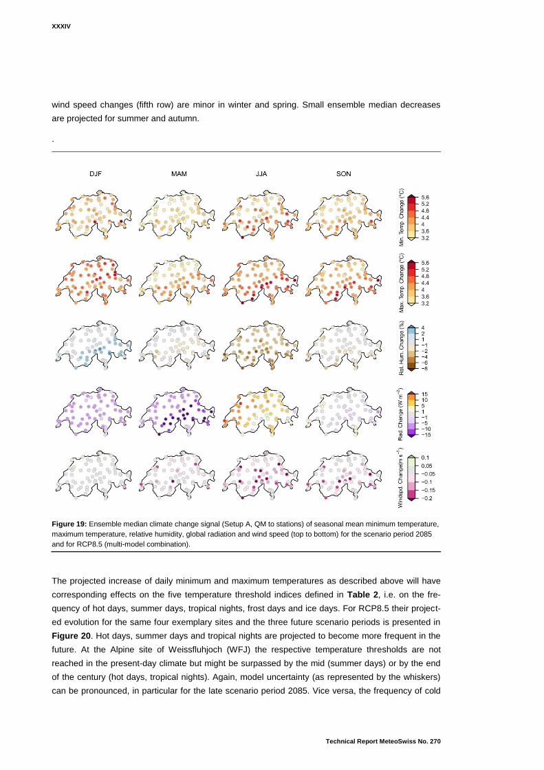
Besides daily mean temperature and precipitation, QM Setup A also considers further meteorological

variables (daily minimum and maximum temperature, relative humidity, global radiation and wind

speed; cf. Table 1). An overview on their projected ensemble median change signals for RCP8.5 and

the late scenario period 2085 is provided by Figure 19. Seasonal mean changes of daily minimum

and maximum temperature (first and second row) show a similar pattern and a similar magnitude as

changes of daily mean temperature (see above). Daily maximum temperature changes, however,

tend to be slightly more pronounced and, in summer and spring, show a characteristic amplification

over the main Alpine ridge. Changes of relative humidity (third row) are small in spring and autumn,

while humidity increases up to several percent are apparent in wintertime over the Alps. In summer,

a decrease of relative humidity by several percent is projected for most parts of the country (in

agreement with, e.g., Sherwood et al. 2010 and Ruosteenoja et al. 2013 for Central Europe). Pro-

jected ensemble median changes of global radiation (fourth row) are negative in winter and spring

and mostly positive in summer, especially north and south of the main Alpine ridge. Autumn shows

little changes. This temporal pattern is strongly connected to the projected precipitation changes (see

above) and cloud cover changes are likely to play a dominant role (not analyzed in detail). Finally,

XXXIV


wind speed changes (fifth row) are minor in winter and spring. Small ensemble median decreases

are projected for summer and autumn.

.

Figure 19: Ensemble median climate change signal (Setup A, QM to stations) of seasonal mean minimum temperature,

maximum temperature, relative humidity, global radiation and wind speed (top to bottom) for the scenario period 2085

and for RCP8.5 (multi-model combination).

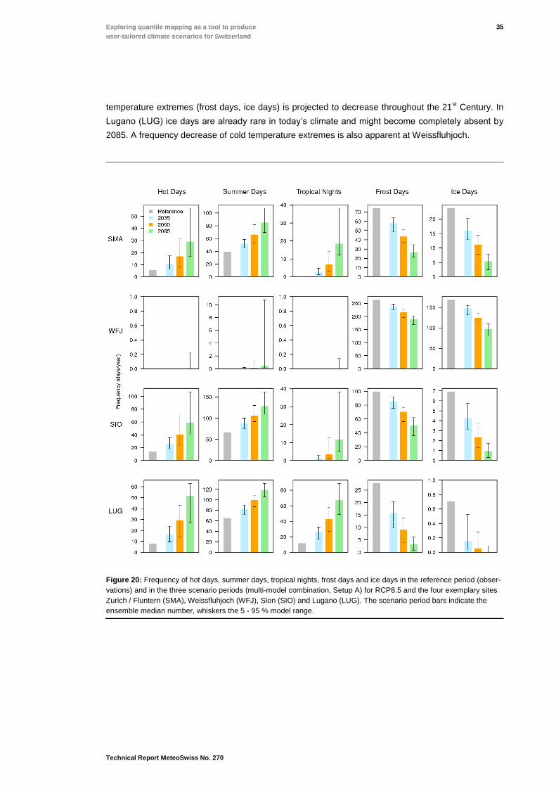
The projected increase of daily minimum and maximum temperatures as described above will have

corresponding effects on the five temperature threshold indices defined in Table 2, i.e. on the fre-

quency of hot days, summer days, tropical nights, frost days and ice days. For RCP8.5 their project-

ed evolution for the same four exemplary sites and the three future scenario periods is presented in

Figure 20. Hot days, summer days and tropical nights are projected to become more frequent in the

future. At the Alpine site of Weissfluhjoch (WFJ) the respective temperature thresholds are not

reached in the present-day climate but might be surpassed by the mid (summer days) or by the end

of the century (hot days, tropical nights). Again, model uncertainty (as represented by the whiskers)

can be pronounced, in particular for the late scenario period 2085. Vice versa, the frequency of cold

35




temperature extremes (frost days, ice days) is projected to decrease throughout the 21st Century. In

Lugano (LUG) ice days are already rare in today’s climate and might become completely absent by

2085. A frequency decrease of cold temperature extremes is also apparent at Weissfluhjoch.

Figure 20: Frequency of hot days, summer days, tropical nights, frost days and ice days in the reference period (obser-

vations) and in the three scenario periods (multi-model combination, Setup A) for RCP8.5 and the four exemplary sites

Zurich / Fluntern (SMA), Weissfluhjoch (WFJ), Sion (SIO) and Lugano (LUG). The scenario period bars indicate the

ensemble median number, whiskers the 5 - 95 % model range.

XXXVI


4 Limitations

Quantile mapping is an attractive and versatile approach for the generation of transient bias-

corrected climate scenarios at different spatial scales. It has a number of advantages compared to

the delta change method that has been employed for the previous CH2011 scenarios (CH2011

2011). However, QM-based products involve a number of limitations and potential pitfalls. Some of

these can speak against the application for specific purposes, and a careful evaluation of the usabil-

ity of QM-based scenarios is required for any given application. In addition, postprocessing by QM

adds another level of uncertainty to the overall uncertainties already inherent to climate model simu-

lations (Wilby and Dessai 2010), in particular for cases where QM is associated with a downscaling

step (here: Setups A and C; Maraun, et al. 2017).

In the following, we provide a brief overview on the limitations of the QM-based products that are

produced and provided to end users in the context of CH2018. Users should make themselves famil-

iar with these restrictions and to assess the usability of the QM-based CH2018 products for their

specific application at hand. Further information can be found in the CH2018 Technical Report and in

the referenced literature.

Stationarity of the model bias: QM is calibrated in the historical reference period and is then ap-

plied to the entire simulated time series including the future scenario period (Figure 2). Hence, QM

implicitly assumes that the calibrated correction function and, consequently, intensity-dependent

climate model biases are stationary in time. Especially under changing climatic conditions this as-

sumption is uncertain (e.g., (Bellprat, et al., 2013), (Buser, et al., 2009), (Maraun, 2013)). Note, how-

ever, that non-stationary biases of simulated mean conditions caused by a systematic shift of the

simulated distribution towards conditions subject to different bias characteristics can be meaningful

and can in principle be accounted for by QM (Ivanov, et al., 2018). QM evaluations employing pseu-

do-realities indicate the validity of the calibrated correction functions also in a future climate (Ivanov &

Kotlarski, 2017).

Temporal variability and remaining biases: QM is a distribution-based correction approach that

does not alter the temporal sequence of the raw climate model output. If climate models have mis-

represented temporal variability (e.g., biased inter-annual or day-to-day variability or biased trends),

remaining biases in the quantile-mapped output are to be expected (Addor and Seibert 2014). Biases

in day-to-day variability can, for instance, arise if large-scale blocking situations and corresponding

circulation regimes over Europe are not well represented by the raw model (e.g. Scaife et al. 2010).

Furthermore and due to the only approximate nature of the QM correction, the quantile-mapped data

can be subject to remaining biases in the calibration period itself even for seasonally averaged val-

ues. These remaining biases are typically small but, in the case of the CH2018 scenarios, can for

instance lead to a systematic underestimation of the observed summer precipitation amounts. This is

the reason why bias correction approaches are nowadays often referred to as bias adjustment, high-

lighting the fact that not all model biases are removed by the correction procedure.

Changes of extremes: The QM correction function for high and low quantiles can be subject to large

uncertainties that partly arise from sampling issues due to a limited number of values considered for

the calibration. Furthermore, the bias of values that lie outside the range of the present-day calibra-

37




tion period (i.e. new extremes that have not been observed in the present-day climate) is not explicit-

ly considered in QM. In our setup, a constant extrapolation of the biases for the 1st and 99

th percen-

tile, respectively, is used (see Chapter 2.2). Other approaches, both parametric and non-parametric,

are possible (e.g., Gutjahr and Heinemann 2013, Ivanov and Kotlarski 2017) and might yield different

results for changes in extremes. The applicability of QM scenarios for assessing changes in ex-

tremes therefore needs to be carefully evaluated, especially for extremes beyond the observed 1st

and 99th percentile, respectively.

Modification of raw climate change signals: The application of QM can modify the raw models’

mean climate change signal and the simulated trends (Themessl et al. 2012, Maurer and Pierce

2014, Gobiet et al. 2015, Casanueva et al. 2018, Ivanov et al. 2018). In the context of CH2018, this

modification is minor in most cases but can be substantial for individual GCM-RCM chains, variables

and meteorological stations/regions. Among others, a systematic and topography-controlled modifi-

cation of the raw models’ temperature change signals by several tenths of a degree by QM was dis-

covered which partly modifies the elevation dependency of the warming signal and to some extent

represents a statistical artifact (see the CH2018 Technical Report for further details). Also relative

precipitation increases in raw model output tend to get amplified by QM, a feature that is directly

connected to the positive precipitation bias of many GCM-RCM chains and the additive nature of the

QM correction. Note that in the presence of intensity dependent model biases these modifications of

the raw climate change signal can be meaningful (Gobiet et al. 2015, Ivanov et al. 2018).

Spatial climate variability: When employed in a downscaling context (here: QM Setups A and C)

QM can misrepresent small scale spatial climate variability on short time scales, e.g. at daily scales

(Maraun 2013). The reason is its deterministic nature when downscaling from coarse climate model

grid cells to local scales and the fact that the predictor information (grid-cell based simulated values)

is translated to finer scales without any randomization that could mimic small-scale variance. The

associated misrepresentation of spatial climate variability at scales finer than the predictor infor-

mation (i.e., smaller than a climate model grid cell) is illustrated, for instance, by Maraun (2013).

Regarding Setup C (QM to high-resolution grid), a further limitation with respect to spatial climate

variability is the observational reference dataset. Its quality depends on the accuracy of the underly-

ing rain-gauge measurements and the capability of the interpolation scheme to reproduce precipita-

tion at ungauged locations. Especially for the observational 2 km precipitation product employed

(MeteoSwiss 2016b), the effective resolution expressed in terms of the typical inter-station distance

(15 to 20 km) is much larger than the nominal 2 km grid spacing. As a consequence, also the quan-

tile-mapped product does not fully represent spatial climate variability at the 2 km scale.

Local-scale processes and feedbacks: QM is a purely empirical and data-driven approach. If ap-

plied in a downscaling context (Setups A and C) it connects coarse-resolution climate model infor-

mation to local-scale conditions without considering the underlying processes that translate a large-

scale signal into its local-scale counterpart. If these processes become modified in a climate change

context, QM cannot account for it as the technique completely relies on the stationarity of the correc-

tion function that is calibrated in a historical reference period. Examples for such processes active in

Alpine terrain are local and regional scale circulation systems (slope and valley winds, Föhn) or ele-

vation-dependent warming signals caused by the snow albedo feedback (Kotlarski et al. 2015, Winter

et al. 2017). See also the comprehensive discussion of these issues by Maraun et al. (2017). Re-

garding elevation-dependent warming, QM-based downscaled projections will furthermore be repre-

XXXVIII


sentative for the elevation of the underlying RCM grid cell and not necessarily for the elevation of the

target station or high-resolution grid cell.

Inter-variable consistency: The QM approach employed in CH2018 is a uni-variate correction and

treats each meteorological variable independently. Therefore, inter-variable consistency in the quan-

tile-mapped products is not given a priori. Previous works have, however, shown that QM generally

maintains inter-variable consistency as represented by the raw RCM output and can to some extent

even correct for biased relations (Wilcke et al. 2013, Ivanov and Kotlarski 2017, Casanueva et al.

2018). An example of the application of QM in a multi-variate context is shown in the CH2018 Tech-

nical Report by means of a heat stress index that is based on temperature and humidity. Neverthe-

less, the CH2018 QM products can be subject to misrepresented inter-variable relations. An obvious

example are individual days on which, for instance, quantile-mapped daily maximum temperature

can be lower than quantile-mapped daily mean or daily minimum temperature at specific stations or

grid cells. The number of these cases is generally small however.

Spatial representativeness: QM to stations (Setup A) uses the simulated output of the climate

model grid cell in which a given station of interest is located as predictor. Similarly, QM to high-

resolution grid (Setup C) employs raw RCM data bi-linearly interpolated to the location of a specific

high-resolution grid cell. In case of a systematically biased spatial variability of the climate model

and, in particular, in case of strong circulation biases, the chosen RCM predictor might not be the

most representative one for deriving scenario projections at the station or high-resolution grid cell of

interest (Maraun and Widmann 2015). In regions of pronounced topography issues of representa-

tiveness can arise, even when systematic climate model biases in spatial variability are absent. This

is solely due to the fact that the climate model topography is only a coarse representation of the true

topography. A given station, for instance, could be located along the northern rim of a ridgeline, while

the overlying climate model grid cell might be located along the southern rim of the coarsened cli-

mate model topography and might, hence, be exposed to different circulation types. Also, in the case

of elevation-dependent forcings such as the snow albedo feedback a nearby climate model grid cell

at similar elevation might be more representative for a given station than the directly overlying grid

cell.

Circulation biases: The presence of large-scale circulation biases in the underlying climate models,

such as a misrepresented frequency of weather types or a systematic dislocation of major storm

tracks, might cause representativeness issues (see above) but could also question the applicability of

QM in general (Maraun and Widmann 2018). QM, by definition, corrects for local to regional-scale

biases but does not consider the nature of these biases and their possible relation to the large-scale

flow regime. Previous works have shown that climate model biases can depend considerably on the

large-scale weather type (Addor et al. 2016, Photiadou et al. 2016). Hence, bias-corrected fields

might be completely inconsistent with the large-scale flow in the underlying climate model, and bias-

corrected fields for a given flow regime might be misrepresented. This potential shortcoming can be

expected to especially affect inter-variable relations (see above) and to introduce artifacts in spatial

climate change patterns. In the context of CH2018, circulation biases of the employed climate mod-

els have not been investigated in detail.

39




5 Summary and Conclusions

This report presents the bias correction and downscaling approach that is employed for the upcom-

ing CH2018 Swiss climate scenarios. The approach largely relies on empirical quantile mapping

(QM), a simple yet versatile method for removing intensity-dependent biases present in raw climate

model output. Three QM setups are employed, two of them (QM to stations and QM to high-

resolution grid) explicitly include a downscaling component. The resulting products provide transient

time series at daily resolution for several meteorological variables and can be directly employed in

subsequent climate impact assessments. This explicitly includes applications that refer to absolute

thresholds of meteorological variables, such as the analysis of frequency changes of days above or

below a certain temperature or precipitation threshold.

A dedicated evaluation of the CH2018 QM implementation reveals a satisfactory performance in the

present-day climate in terms of an effective removal of mean model biases. Still, remaining biases

might be present for extremes, for daily to interannual climate variability, for small-scale spatial cli-

mate variability, for inter-variable relations and to some extent even for seasonal climatologies. Simi-

lar to all other downscaling and bias correction methods, QM has a range of potential limitations and

might not be applicable to all kinds of climate impact research. These limitations mostly originate

from the fact that QM is a purely statistical and data-driven method. It does not incorporate physical-

ly-based knowledge on the processes that are responsible for either model biases or for small-scale

climate variability beyond the scale resolved by the underlying climate models. These potential limita-

tions are summarized in Chapter 4. They often especially arise in topographically structured terrain

where spatial climate variability is large and relevant processes are not or only approximately cap-

tured by climate models. Also note that the QM-based scenarios are subject to modeling and emis-

sion scenario uncertainties as represented by the projection range of the model ensemble at hand.

As a consequence, users of the QM-based scenarios should properly address the uncertainty

sources and should assess the validity of the datasets for each specific application.

XL


Acknowledgment

The present work represents a collaborative effort that was mainly carried out by the author and the

co-authors of the study, but that was strongly supported by further persons. This especially concerns

the preparation and harmonization of climate model and observational data by Curdin Spirig (C2SM),

Jan Rajczak (ETH Zurich/MeteoSwiss) and Urs Beyerle (ETH Zurich). Strong technical support was

provided by Felix Maurer and Rebekka Posselt (both MeteoSwiss). Jan Rajczak, Kuno Strassmann

(C2SM) and Jonas Bhend (MeteoSwiss) provided extremely useful scientific input. Jan Rajczak pro-

vided further useful comments during an internal review of the report. Finally, we thank the entire

CH2018 consortium and especially the CH2018 working group on downscaling for their feedback and

their suggestions in numerous project meetings and discussions.

References

Addor, N., Rohrer, M., Furrer, R. and Seibert, J., 2016. Propagation of biases in climate models from

the synoptic to the regional scale: Implications for bias adjustment. Journal of Geophysical Research,

Volume 121.

Addor, N. and Seibert, J., 2014. Bias correction for hydrological impact studies – beyond the daily

perspective. Hydrological Processes, 28, 4823-4828.

Bellprat, O., Kotlarski, S., Lüthi, D. and Schär, C., 2013. Physical constraints for temperature biases

in climate models. Geophysical Research Letters, 40, 4042-4047.

Boé, J., Terray, L., Habets, F. and Martin, E., 2007. Statistical and dynamical downscaling of the

Seine basin climate for hydro-meteorological studies. International Journal of Climatology, 27, 1643-

1655.

Bosshard, T., Kotlarski, S., Ewen, T. and Schär, C., 2011. Spectral representation of the annual cycle

in the climate change signal. Hydrology and Earth System Sciences, 15, 2777-2788.

Buser, C. M., Künsch, H. R., Lüthi, D., Wild, M. and Schär, C., 2009. Bayesian multi-model projection

of climate: bias assumptions and interannual variability. Climate Dynamics, 33, 849-868.

Casanueva, A., Bedia, J., Herrera, S., Fernández, J. and Gutiérrez, J. M., 2018. Direct and

component-wise bias correction of multi-variate climate indices: the percentile adjustment function

diagnostic tool. Climatic Change, 147, 411-425.

CH2011, 2011. Swiss Climate Change Scenarios CH2011. Published by C2SM, MeteoSwiss, ETH,

NCCR Climate, and OcCC, Zurich, Switzerland, 88 pp. Available from www.ch2011.ch.

Déqué, M., Rowell, D. P., Lüthi, D., Giorgi, F., Christensen, J.H., Rockel, B., Jacob, D., Kjellström, E.,

de Castro, M. and van den Hurk, B., 2007. An intercomparison of regional climate simulations for

Europe: assessing uncertainties in model projections. Climatic Change, 81, 53-70.

41




Fowler, H. J., Blenkinskop, S. and Tebaldi, C., 2007. Linking climate change modelling to impacts

studies: recent advances in downscaling techniques for hydrological modelling. International Journal

of Climatology, 27, 1547-1578.

Gobiet, A., Suklitsch, M. and Heinrich, G., 2015. The effect of empirical-statistical correction of

intensity-dependent model errors on the climate change signal. Hydrology and Earth System

Sciences, 19, 4055-4066.

Gudmundsson, L., Bremnes, J. B., Haugen, J. E. and Engen-Skaugen, T., 2012. Technical Note:

Downscaling RCM precipitation to the station scale using statistical transformations – a comparison

of methods. Hydrology and Earth System Sciences, 16, 3383-3390.

Gutiérrez, J. M. et al., 2018. An intercomparison of a large ensemble of statistical downscaling

methods over Europe: Results from the VALUE perfect predictor cross-validation experiment.

International Journal of Climatology, in press.

Gutjahr, O. and Heinemann, G., 2013. Comparing precipitation bias correction methods for high-

resolution regional climate simulations using COSMO-CLM. Theoretical and Applied Climatology,

114, 511-529.

Haylock, M. R. et al., 2008. A European daily high-resolution gridded data set of surface temperature

and precipitation for 1950–2006. Journal of Geophysical Research, 113, D20119.

Herger, N., Sanderson, B. M. and Knutti, R., 2015. Improved pattern scaling approaches for the use

in climate impact studies. Geophysical Research Letters, 42, 3486–3494.

Isotta, F. et al., 2014. The climate of daily precipitation in the Alps: development and analysis of a

high-resolution grid dataset from pan-Alpine rain-gauge data. International Journal of Climatology,

34, 1657-1675.

Ivanov, M. A., Luterbacher, J. and Kotlarski, S., 2018. Climate Model Biases and Modification of the

Climate Change Signal by Intensity-Dependent Bias Correction. Journal of Climate, in press.

Ivanov, M. and Kotlarski, S., 2017. Assessing distribution-based climate model bias correction

methods over an alpine domain: added value and limitations. International Journal of Climatology,

37, 2633-2653.

Jacob, D. et al., 2014. EURO-CORDEX: new high-resolution climate change projections for

European impact research. Regional Environmental Change, 14, 563-578.

Kotlarski, S., Ivanov, M. and Schär, C., 2017. Bias-corrected transient scenarios at the local scale

and at daily resolution. CH2011 Extension Series No. 4, 21 pp. Available from www.ch2011.ch.

Kotlarski, S. et al., 2014. Regional climate modeling on European scales: a joint standard evaluation

of the EURO-CORDEX RCM ensemble. Geoscientific Model Development, 7, 1297-1333.

Kotlarski, S., Lüthi, D. and Schär, C., 2015. The elevation dependency of 21st century European

climate change: an RCM ensemble perspective. International Journal of Climatology, 35, 3902-3920.

Maraun, D., 2013. Bias Correction, Quantile Mapping, and Downscaling: Revisiting the Inflation

Issue. Journal of Climate, 26, 2137-2143.

Maraun, D., 2016. Bias Correcting Climate Change Simulations - a Critical Review. Current Climate

Change Reports, 2, 211-220.

Maraun, D. et al., 2017. Towards process-informed bias correction of climate change simulations.

Nature Climate Change, 7, 764-773.

Maraun, D. et al., 2010. Precipitation downscaling under climate change: Recent developments to

bridge the gap between dynamical models and the end user. Reviews of Geophysics, 48, RG3003.

XLII


Maraun, D. and Widmann, M., 2015. The representation of location by a regional climate model in

complex terrain. Hydrology and Earth System Sciences, 19, 3449-3456.

Maraun, D. and Widmann, M., 2018. Statistical Downscaling and Bias Correction for Climate

Research. Cambridge University Press.

Maurer, E. P. and Pierce, D. W., 2014. Bias correction can modify climate model simulated

precipitation changes without adverse effect on the ensemble mean. Hydrology and Earth System

Sciences, 18, 915-925.

MeteoSwiss, 2016a. Documentation of MeteoSwiss Grid-Data Products. Daily Mean, Minimum and

Maximum Temperature: TabsD, TminD, TmaxD. MeteoSwiss. Available from

https://www.meteoswiss.admin.ch/content/dam/meteoswiss/de/service-und-

publikationen/produkt/raeumliche-daten-temperatur/doc/ProdDoc_TabsD.pdf.

MeteoSwiss, 2016b. Documentation of MeteoSwiss Grid-Data Products. Daily Precipitation (final

analysis): RhiresD. MeteoSwiss. Available from

https://www.meteoswiss.admin.ch/content/dam/meteoswiss/de/service-und-

publikationen/produkt/raeumliche-daten-niederschlag/doc/ProdDoc_RhiresD.pdf.

Monhart, S., Sprigi, C., Bhend, J., Bogner, K. and Schär, C., 2018. Skill of Subseasonal Forecasts in

Europe: Effect of Bias Correction and Downscaling Using Surface Observations. Journal of

Geophysical Research: Atmospheres, in press.

Moss, R. H. et al., 2010. The next generation of scenarios for climate change research and

assessment. Nature, 463, 747-756.

Panofsky, H. A. and Brier, G. W., 1968. Some Applications of Statistics to Meteorology. Earth and

Mineral Sciences Continuing Education, College of Earth and Mineral Sciences.

Photiadou, C., Hurk, B., Delden, A. and Weerts, A., 2016. Incorporating circulation statistics in bias

correction of GCM ensembles: hydrological application for the Rhine basin. Climate Dynamics, 46,

187-203.

Piani, C., Haerter, J. and Coppola, E., 2010. Statistical bias correction for daily precipitation in

regional climate models over Europe. Theoretical and Applied Climatology, 99, 187-192.

Rajczak, J., Kotlarski, S., Salzmann, N. and Schär, C., 2016a. Robust climate scenarios for sites with

sparse observations: a two-step bias correction approach. International Journal of Climatology, 36,

1226-1243.

Rajczak, J., Kotlarski, S. and Schär, C., 2016b. Does quantile mapping of simulated precipitation

correct for biases in transition probabilities and spelllengths? Journal of Climate, 29, 1605-1615.

Ruosteenoja, K. and Räisänen, P., 2013. Seasonal Changes in Solar Radiation and Relative

Humidity in Europe in Response to Global Warming. Journal of Climate, 26, 2467-2481.

Scaife, A. A. et al., 2010. Atmospheric Blocking and Mean Biases in Climate Models. Journal of

Climate, 23, 6143-6152.

Sevruk, B., 1997. Regional dependency of precipitation-altitude relationship in the Swiss Alps.

Climatic Change, 36, 355-369.

Sherwood, S. C. et al., 2010. Relative humidity changes in a warmer climate. Journal of Geophysical

Research, 114, D09104.

Themessl, M., Gobiet, A. and Heinrich, G., 2012. Empirical-statistical downscaling and error

correction of regional climate models and its impact on the climate change signal. Climatic Change,

112, 449-468.

43




Themessl, M. J., Gobiet, A. and Leuprecht, A., 2011. Empirical-statistical downscaling and error

correction of daily precipitation from regional climate models. International Journal of Climatology, 31,

1530-1544.

Wetterhall, F., Pappenberger, F., He, Y., Freer, J. and Cloke, H. L., 2012. Conditioning model output

statistics of regional climate model precipitation on circulation patterns. Nonlinear Processes in

Geophysics, 19, 623-633.

Wilby, R. L. and Dessai, S., 2010. Robust adaptation to climate change. Weather, 65, 180-185.

Wilby, R. L. and Fowler, H. J., 2011. Regional Climate Downscaling. In: F. Fung, A. Lopez & M. New:

Modelling the Impact of Climate Change on Water Resources. Blackwell Publishing Ltd., 34-85.

Wilby, R. L. and Wigley, T. M. L., 2000. Precipitation predictors for downscaling: Observed and

general circulation model relationships. International Journal of Climatology, 20, 641-661.

Wilcke, R. A., Mendlik, T. and Gobiet, A., 2013. Multi-variable error correction of regional climate

models. Climatic Change, 120, 871-887.

Winter, K. J.-P. M., Kotlarski, S., Scherrer, S. C. and Schär, C., 2017. The Alpine snow-albedo

feedback in regional climate models. Climate Dynamics, 48, 1109-1124.

MeteoSchweiz

Operation Center 1

CH-8044 Zürich-Flughafen

T +41 58 460 99 99

www.meteoschweiz.ch

MeteoSvizzera

Via ai Monti 146

CH-6605 Locarno Monti

T +41 58 460 97 77

www.meteosvizzera.ch

MétéoSuisse

7bis, av. de la Paix

CH-1211 Genève 2

T +41 58 460 98 88

www.meteosuisse.ch

MétéoSuisse

Chemin de l’Aérologie

CH-1530 Payerne

T +41 58 460 94 44

www.meteosuisse.ch

Documents

Technical Report MeteoSwiss No. 270 Exploring quantile ... · that reflect the spatial and temporal scale of the underlying observations. The local daily product of the CH2011 scenarios