Embed Size (px)
Citation preview

Technical Report
May 2020
Performance Based Seismic Design of
Lateral Force Resisting System
Prepared by: Dr.-Eng. Kenan Michel
This report has been prepared at the end of the “ongoing phase” spent at the University of California in San Diego by the Experienced Researcher Kenan Michel, as part of CIC-BREL project (Cracked and Inelastic Calculation of BRacing ELements). This project has received funding from the European Union’s Horizon 2020 research and innovation program under agreement No 744332 – CIC – BREL.

Page 1
Table of Contents:
Acknowledgement 4
PART I: General Information, Site and Loading 5
1. General Information About the Building 5
1.1. Specified Material Properties: 6
1.2. Site Information: 6
1.3. Geometry (Figure I.1): 7
2. Site Seismicity and Design Coefficients 7
2.1. USGS Results 7
2.2. Site Response Spectra 8
2.3. Design Coefficients And Factors For Seismic Force-Resisting Systems 8
3. Loading 9
3.1. Determination Of Seismic Forces 9
3.2. Modal Response Spectrum Analysis 9
3.3. Seismic Load Effects And Combinations 11
PART II: Core Wall Design - Linear Model 12
4. Model of ETABS 12
4.1. Geometry 12
4.2. Gravity Loads 13
4.3. Seismic Loads 15
4.4. Tabulated Selected Results From ETABS Analysis 16
5. P-M Interaction Diagrams 17
5.1. N-S Direction 17
5.2. E-W Direction 19
6. Lateral Force Resisting System, Linear 20
6.1. Longitudinal Reinforcement 20
6.2. Shear Reinforcement 22
6.3. Boundary Elements 24
6.3.1. Transverse Reinforcement Of Boundary Elements 26
6.4. Coupling Beams 27
7. Detailing 30
PART III: Site Response Spectra and Input Ground Motions 31

Page 2
8. Performance Levels 31
8.1. ASCE 7-16 Target Spectra 31
8.2. Site Response Spectra 34
8.2.1. Ground Motion Conditioning 34
8.2.2. Amplitude Scaling 37
8.2.3. Pseudo Acceleration and Displacement Response Spectra 38
PART IV: Non-Linear Model 40
9. Variant 1 of Non-Linear Model 40
9.1. Complete Core Wall Design for Combined Axial-Flexure 40
9.2. Modal Analysis 43
9.3. Influence of the Damping Model on the Nonlinear Dynamic Response 49
10. Variant 2 of Non-Linear Model 57
10.1. Influence of the Coupling Beam Model on the Nonlinear Dynamic Response 57
10.2. Estimated Roof Displacement 68
PART V: Design Verification 70
11. General 70
11.1. Performance Objectives 70
11.2. Model For Time-History Analyses 71
11.3. Performance Level Verification 71
11.4. Fully Operational Performance Level Verification 71
11.5. Life Safety Performance Level Verification 78
PART VI: Capacity Design of Force Controlled Elements and Regions and Design of Acceleration-
Sensitive Nonstructural Elements 87
12. General 87
12.1. Design Verification 87
12.1.1. Full Occupancy Case 87
12.1.2. Life Safety Case 91
12.1.3. Observations on Plots 93
12.2. Acceleration response spectra at roof level 94
12.2.1. Observations on Plots 95
12.3. Core Wall 97
12.4. Design Detail Comparison 103
12.5. Detailed Drawing 103

Page 3
12.6. Diaphragm 104
12.7. Fire Sprinkler System 117
12.8. Overhanging Projector 119
PART VII: Conclusion 122

Page 4
Acknowledgement This project has been carried out mainly under the guidance of Professor José Restrepo
and commendable mentoring of Rodolfo Sanchez, Teaching Assistant.
Basic information and a lot of support are taken from the classes of Prof. Benson Shing
in the class Earthquake Engineering and Prof. Joel Conte in the class Nonlinear
Structural Analysis.
I would also like to thank the Department of Structural Engineering, UCSD for availing
this opportunity to learn these coursed.
Moreover, fellow classmates, Molly Pobiel and Dhyey Bhavsar played an important role
in developing and writing some parts of this report when working as a project team, I
highly appreciate their contribution and work.

Page 5
PART I: General Information, Site and Loading
1. General Information About the Building
A fourteen-story residential building will be constructed in Downtown LA, California. A typical plan view of the building is shown in Figure I.1. Floor to floor height is 12’ for all floors except for the first level, in which the story height is 16’. The North-South (N-S) and East-West (E-W) lateral force resisting system for the building consists of one core wall. Since the core wall will be framing the elevator shafts and stairwells, the architect provided specific centerline dimensions for the walls. The specified centerline length of the walls is 10’-6” in the E-W direction and 24’ in the N-S direction, with a wall thickness of 30” at stories 1-5 and 22” at stories 6-14, as shown in Figure I.2. The coupling beams spanning 7’ between the c-shaped walls are 42” deep with the same width of the walls. The slabs are 8” reinforced concrete supported by 28” square columns. The contribution to the lateral resistance from the gravity framing system will be ignored. For this project, the lateral force resisting system in the N-S and E-W directions will be designed and detailed. The model of ETABS will was already provided.
Figure I.1 Typical Floor Framing Plan

Page 6
Figure I.2 Typical core wall plan view and dimensions.
Note: wall thickness t = of 30” at stories 1-5 and t = 22” at stories 6-14.
1.1. Specified Material Properties:
Concrete compressive strength (cylinder): f’c = 7 ksi Concrete unit weight: w =150 pcf Steel reinforcement yield strength Grade 60 ASTM A615: fy = 60 ksi
1.2. Site Information:
Location coordinates: 34.05° N, 118.26° W 550 South Hope St, Los Angeles, CA 90071 (Downtown LA) Site soil class: D “Stiff soil” Code reference document: ASCE 7-16 Risk category: non-essential facility (II), Ie=1.0

Page 7
1.3. Geometry (Figure I.1):
Typical floor height = 12’ First floor height = 16’ RC concrete slab thickness = 8” Columns = 28”x28” square (maximum stress from unfactored DL < 0.25*(f’c) Wall centerline dimensions: 24’ NS, 10’-6” EW, t= 30” (stories 1-5) - 22” (stories 6-14) Coupling beam dimensions: 30”-22” wide x 42” deep (Figure I.2)
2. Site Seismicity and Design Coefficients
2.1. USGS Results
Site information was input into USGS website (Figure I.3) to obtain the mapped acceleration parameters per ASCE 7-16 §11.4.1.
Figure I.3 Map of site location. Location coordinates: 34.05° N, 118.26° W
Mapped acceleration parameters
Ss=1.966 g SMS=1.970 g SDS=2/3* Ss = 1.311 g
S1=0.700 g SM1=1.190 g SD1=2/3* S1 = 0.793 g
Seismic Design Category E
Page 8
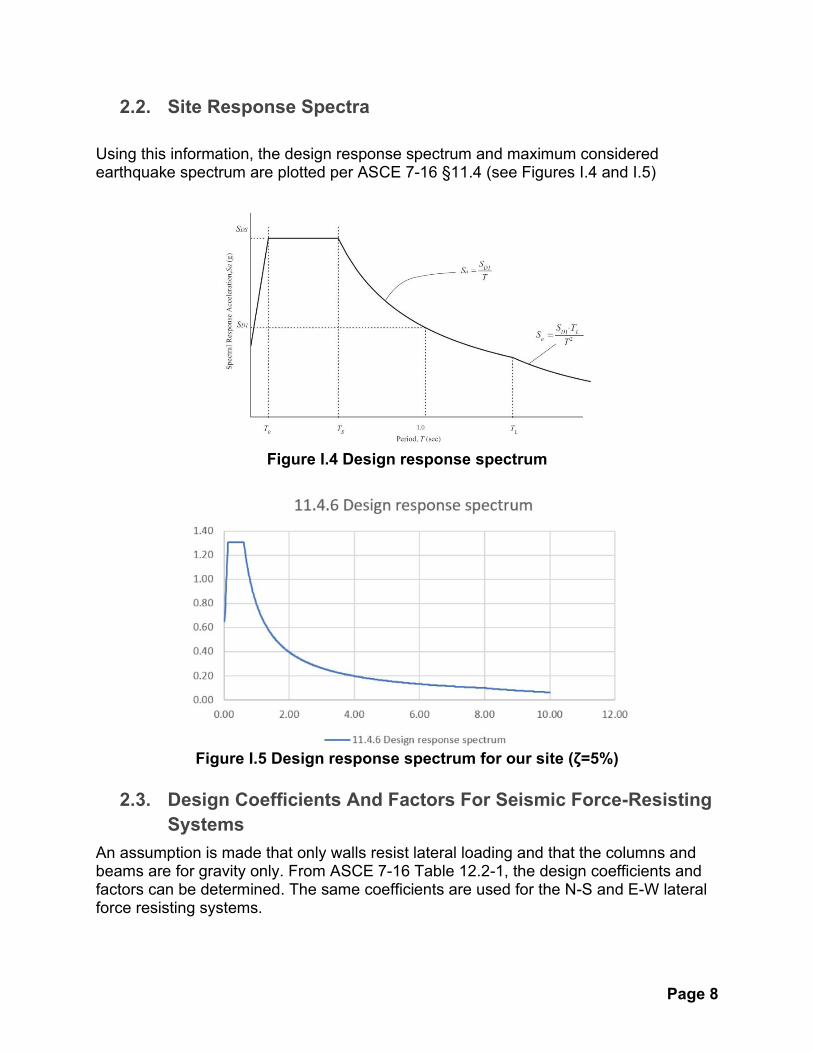
2.2. Site Response Spectra
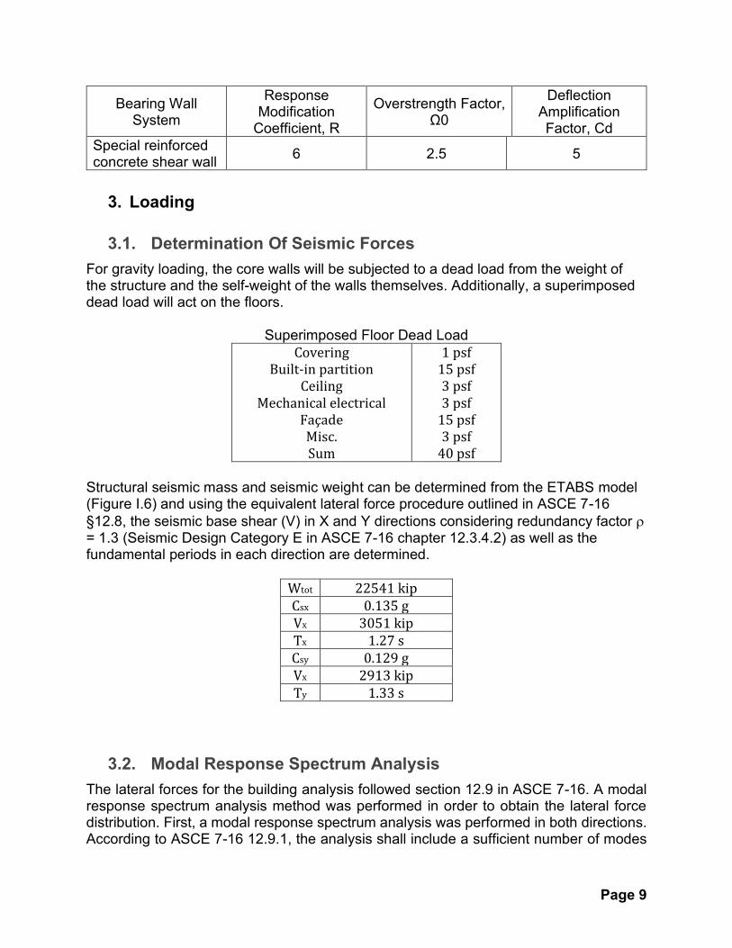
Using this information, the design response spectrum and maximum considered earthquake spectrum are plotted per ASCE 7-16 §11.4 (see Figures I.4 and I.5)
Figure I.4 Design response spectrum
Figure I.5 Design response spectrum for our site (ζ=5%)
2.3. Design Coefficients And Factors For Seismic Force-Resisting
Systems
An assumption is made that only walls resist lateral loading and that the columns and beams are for gravity only. From ASCE 7-16 Table 12.2-1, the design coefficients and factors can be determined. The same coefficients are used for the N-S and E-W lateral force resisting systems.
Page 9
Bearing Wall System
Response Modification
Coefficient, R
Overstrength Factor, Ω0
Deflection Amplification Factor, Cd
Special reinforced concrete shear wall
6 2.5 5
3. Loading
3.1. Determination Of Seismic Forces
For gravity loading, the core walls will be subjected to a dead load from the weight of the structure and the self-weight of the walls themselves. Additionally, a superimposed dead load will act on the floors.
Superimposed Floor Dead Load
Covering Built-in partition
Ceiling Mechanical electrical
Façade Misc. Sum
1 psf 15 psf 3 psf 3 psf
15 psf 3 psf
40 psf Structural seismic mass and seismic weight can be determined from the ETABS model (Figure I.6) and using the equivalent lateral force procedure outlined in ASCE 7-16
§12.8, the seismic base shear (V) in X and Y directions considering redundancy factor = 1.3 (Seismic Design Category E in ASCE 7-16 chapter 12.3.4.2) as well as the fundamental periods in each direction are determined.
Wtot 22541 kip
Csx 0.135 g
Vx 3051 kip
Tx 1.27 s
Csy 0.129 g
Vx 2913 kip
Ty 1.33 s
3.2. Modal Response Spectrum Analysis
The lateral forces for the building analysis followed section 12.9 in ASCE 7-16. A modal response spectrum analysis method was performed in order to obtain the lateral force distribution. First, a modal response spectrum analysis was performed in both directions. According to ASCE 7-16 12.9.1, the analysis shall include a sufficient number of modes

Page 10
to obtain a combined modal mass participation of at least 90% of the mass in each direction, a maximum of 30 modes were computed in the ETABS model with such purpose. Modes 2 and 1 for the E-W and N-S respectively resulted the fundamental periods in each direction. The corresponding base shears Vtx and Vty, were obtained and compared to 100% of the base shear obtained from the equivalent lateral force procedure. Vt in both directions was found to be less than V from ELF procedure, so the forces were increased by Vx/Vtx and Vy/Vty, for the E-W and N-S directions, respectively.
EW (X) NS (Y)
Mode Period (s) Mode Period (s)
2 1.27 1 1.33
Vtx: 2446 kip < Vx = 3051 kip Vty: 2308 kip < Vy = 2913 kip
Amplification factor
Vx /Vtx: 1.25 Vy /Vty: 1.26
Figure I.6 Model of ETABS
Page 11
3.3. Seismic Load Effects And Combinations
The seismic load effect, E, is defined in ASCE 7-16 §12.4.2 as:
E = Eh + Ev or E = Eh - Ev (depending on the load combination) where horizontal seismic load effect is defined by ASCE 7-16 §12.4.2.1 as:
Eh = QE
Per §12.3.4.2, the redundancy factor, , is taken as 1.3. The vertical seismic load effect is defined by §12.4.2.1 as:
Ev = 0.2SDSD The basic combinations used for this analysis are defined by §2.3.2:
1.2D + 1.0E + 1.0L 0.9D + 1.0E
or as defined by §2.3.6 equations 6 and 7as:
1.2D + Eh + Ev + 1.0L + 0.2S 0.9D + Eh - Ev
Substituting the values for E into the loading combinations:
(1.2 + 0.2SDS) D+L ±1.0Eh
(0.9 - 0.2SDS) D ± 1.0Eh Using SDS = 1.311, the final seismic load combinations used for analysis are:
(1.462) D +L ±1.0Eh (0.638 D) ±1.0Eh

Page 12
PART II: Core Wall Design - Linear Model
4. Model of ETABS
4.1. Geometry
The analysis was run with stiffness modifiers equal to 0.5*Ig in both c-shaped walls,
according with the suggested for the ACI 318-14, whereas the coupling beams used
stiffness modifiers equal to 0.3*Ig.
Note: From that analysis, the trailing wall experiences tensile axial force from lateral
loading in the E-W direction. Since the shear capacity of the wall is greatly reduced if it is
experiencing a tensile axial force, spurious shear distribution between trailing and leading
walls is expected in the linear analysis.
Figure II.1 Extruded elevation of the corewall

Page 13
4.2. Gravity Loads
Figure II.2 Typical plan view of model.
Figure II.3 Elevation D (left) and Elevation 2(right)

Page 14
Figure II.4 Superimposed dead load (SDL) (ksf).
Figure II.5 Live load (Live) (ksf).
Note: Dead load (Dead) from self-weight is consider automatically in the ETABS model.

Page 15
4.3. Seismic Loads
Unless otherwise indicated, results will be presented in kips (k) and kip-feet (k-ft). A
positive axial load is tension, and a negative axial load is compression. The sign
convention for the moments is shown in Figure II.6.
(a) Mu,NS
(b) Mu,EW
Figure II.6 Sign convention
X (+)
Y (+)

Page 16
4.4. Tabulated Selected Results From ETABS Analysis
Moments NS and shear forces EW at the base of the C-shaped wall at the left.
No LC Pu (kip)
Mu, NS (kip-ft)
Vu, EW (kip)
u/hw
1 0.9D - 0.2SDS + 1.0EX Max 7384 33485 1529 0.0060 2 0.9D - 0.2SDS + 1.0EX Min -14767 -33151 -1480 0.0060 3 1.2D + 0.2SDS + 0.5L + 1.0EX Max 2146 33724 1564 0.0060 4 1.2D + 0.2SDS + 0.5L + 1.0EX Min -20005 -32912 -1445 0.0060 Notes: Pu (-) is compression in the C-shaped wall. For sign convention of Mu see Figure II.6. If Vu, EW is (+) the shear force goes to the East. Moments EW and shear forces NS at the base of the C-shaped wall at the left.
No
LC Pu (kip)
Mu, NS (kip-ft)
Vu, EW (kip)
u/hw
1 0.9D - 0.2SDS + 1.0EX Max -3691 144880 1442 0.0066 2 0.9D - 0.2SDS + 1.0EX Min -3691 -144880 -1442 0.0066 3 1.2D + 0.2SDS + 0.5L + 1.0EX Max -8930 144880 1442 0.0066 4 1.2D + 0.2SDS + 0.5L + 1.0EX Min -8930 -144880 -1442 0.0066 Notes: Pu (-) is compression in the C-shaped wall. For sign convention of Mu see Figure II.6. If Vu, NS is (+) the shear force goes to the North.
Shear forces in the coupling beams (face N or S)
Story
0.9D - 0.2SDS + 1.0EX
Vu (kip)
1.2D + 0.2SDS + 0.5L + 1.0EX
Vu (kip)
14 131 134
13 192 195
12 260 263
11 322 325
10 372 375
9 413 416
8 447 450
7 474 477
6 486 489
5 611 615
4 620 624
3 626 630
2 606 610
1 508 512

Page 17
5. P-M Interaction Diagrams
A P-M interaction diagram in excel is developed for C shape core wall for both cases of
loading, N-S and EW. Each of them covers the case when the bending moment is
positive and negative.
5.1. N-S Direction
For N-S loading, input data and the geometry are shown in figure II.7
Figure II.7 C shape core wall, geometry and material in N-S direction
For the N-S direction, when putting the values of Pu and Mu,NS we get a maximum
reinforcement ratio of 1.4% as shown in table II.1 and figure II.8. In figure II.8, the limit
values of Pu and Mu,NS are shown in red dots.
f'c ksi 7
fy ksi 60
Es ksi 29000
Lw1 in 141
Lw2 in 318
t1 in 30
t2 in 30
β1 0.70
Ag in2 16200
x̅ in 43.98
x1 in 15
x2 in 35.25
x3 in 105.75
xs̅ in 44.0
ρ 0.40%
As1 in2 31.0
As2 in2 8.5
As3 in2 8.5
Ast in2 64.8
Lw1
Lw2
t1
t1
t2
As1
As2 As3
As2 As3
i Asi xi----------------------1 As1 t2/22 As2 Lw1/43 As3 3Lw1/4

Page 18
Table II.1 Loads and required reinforcement ratios, C shape wall in N-S direction
Figure II.8 P-M Interaction diagram, C shape wall in N-S direction
Load / No. LC 1 LC 2 LC 3 LC 4
Pu 7384 -14767 2146 -20005
Mu,ns 33485 -33151 33724 -32912
Vu,ew 1529 -1480 1564 -1445
δu / hw 0.0066 0.0066 0.0066 0.0066
cMax 23.74 23.74 23.74 23.74
ro required 1.4 0.4 0.8 0.4
ro max 1.4 1.4 1.4 1.4
c [inch] 4 12.9 25 18
Boundary no no yes no

Page 19
5.2. E-W Direction
In E-W direction the input values and geometry are shown in figure II.9.
Figure II.9 C shape core wall, geometry and material in E-W direction
For the E-W direction, we the values of Pu and Mu,EW we get a maximum reinforcement
ratio of 1.0% as shown in table II.2 and figure II.10. In figure II.10, the limit values of Pu
and Mu,EW are shown in red dots.
Table II.2 – Loads and required reinforcement ratios, C shape wall in E-W
direction
f'c ksi 7
fy ksi 60
Es ksi 29000
Lw1 in 141
Lw2 in 318
t1 in 30
t2 in 30
β1 0.70
Ag in2 16200
y̅ in 159.00
y1 in 15
y2 in 79.5
y3 in 238.5
y4 in 303
ρ 0.40%
As1 in2 13.3
As2 in2 19.1
As3 in2 19.1
As4 in2 13.3
Ast in2 64.8
Lw1
Lw2
t1
t1
t2
As2
As1
As3
As4
=Lw2/2
i Asi yi----------------------1 As1 t1/22 As2 Lw2/43 As3 3Lw2/44 As4 Lw2-t1/2
Load / No. LC 1 LC 2 LC 3 LC 4
Pu -3691 -3691 -8930 -8930
Mu,ns 144880 -144880 144880 -144880
Vu,ew 1442 -1442 1442 -1442
δu / hw 0.006 0.006 0.006 0.006
cMax 26.11 58.89 58.89 58.89
ro required 1 0.4 0.4 1
ro max 1 1 1 1

Page 20
Figure II.10 P-M Interaction diagram, C shape wall in E-W direction
6. Lateral Force Resisting System, Linear
6.1. Longitudinal Reinforcement
The dimensions of the shear wall are already given thus the next step in designing the
shear walls is to determine the required longitudinal reinforcement. From the P-M
envelopes developed before. The demands are plotted in red in figures II.8 for NS and
figure II.10 for EW directions.
The required reinforcement ratio in the N-S direction 𝜌𝑙 max𝑁𝑆 was found 1.4%, see figure
II.8 and table II.1. The required longitudinal reinforcement ratio in E-W direction
𝜌𝑙 max𝐸𝑊was found to be 1%, see figure II.10 and table II.2. The required reinforcement
ratio is then {max (𝜌𝑙 max𝐸𝑊 , 𝜌𝑙 max𝑁𝑆)=1.4 %} for the whole cross section.
This value is bigger than the minimum longitudinal reinforcement ratio of 0.25% per ACI
318-14 chapter. 18.10.2.1 and the minimum reinforcement ratio of 0.42% per chapter.
9.6.1.2. It is also less than the maximum reinforcement ratio of 2.5% per chapter 18.6.3.1.
Choosing the required bars is done in both directions N-S and E-W. In N-S direction the
shape and required reinforcement areas are shown in figure II.11
144880, -3691-144880, -3691
144880, -8930-144880, -8930
-18000
-14000
-10000
-6000
-2000
2000
6000
10000
14000
-320000 -280000 -240000 -200000 -160000 -120000 -80000 -40000 0 40000 80000 120000 160000 200000 240000 280000 320000
Des
ign
Axi
al L
oa
d φ
Pn
or
Dem
an
d P
u(k
ip)
Design Moment φMn or Demand Mu (kip-ft)
0.4%
ρl = 1.8%
c/lw2 = 0.04
0.021
0.0
0.021
0.07
0.04
0.07

Page 21
Figure II.11 Required reinforcement areas for N-S direction
In E-W direction the shape and required reinforcement areas are shown in figure II.12
Figure II.12 Required reinforcement areas for E-W direction
Lw1 in 141
Lw2 in 318
t1 in 30
t2 in 30
Required
ρ 1.40%
As1 in2 108.4
As2 in2 29.6
As3 in2 29.6
Ast in2 226.8
As1 84 # 10 in2 106.7
As2 24 # 10 in2 30.5
As3 24 # 10 in2 30.5
Ast in2 228.6
Chosen
NS directionLw1
Lw2
t1
t1
t2
As1
As2 As3
As2 As3
Lw1 in 141
Lw2 in 318
t1 in 30
t2 in 30
Required
ρ 1.40%
As1 in2 46.6
As2 in2 66.8
As3 in2 66.8
As4 in2 46.6
Ast in2 226.8
As1 38 # 10 in2 48.3
As2 52 # 10 in2 66.0
As3 52 # 10 in2 66.0
As4 38 # 10 in2 48.3
Ast in2 228.6
Chosen
EW directionLw1
Lw2
t1
t1
t2
As2
As1
As3
As4

Page 22
By considering both directions, with the available perimeter of the section to distribute
the bars on it, the resulting longitudinal reinforcement should look like the figure II.13:
Figure II.13 Distributing longitudinal bars in the section, and bar spacing
6.2. Shear Reinforcement
The procedure to design the c-shape wall for shear is shown as follows:
• According to ACI 318-14, chapter 18.10.2.2 two curtain of shear reinforcement will be
used.
• According to ACI 318-14, chapter 18.10.2.3 development length are defined in table II.3:
Lw2-2t1= 258 inch
2*(Lw2-2t1)= 516 inch OK
S o.c. = 6.3 inch
S = 5.0 inch
Lw1/2 70.5 inch Lw1/2 70.5 inch
2*Lw1/2-t2 111 inch 2*Lw1/2+t1 171 inch
S o.c.= 4.8 inch S o.c. = 7.4 inch
S = 3.6 inch S = 6.2 inch
Lw1
Lw2
t1
t1
t2
As184#10
As2 As3
As2As3
10#10
10#10
14#10
14#10
24#10
24#10

Page 23
Table II.3 – Development length calculation of long. Reinf.
>> Development length 113” (in the foundation)
• According to ACI 318-14, chapter 18.10.3 shear demand and the parts of the c-shape
wall that carry the shear in each direction are shown in table II.4:
Table II.4 – Shear demand and section geometry
• According to ACI 318-14, chapter 18.10.4 shear capacity and the design of shear
reinforcement is shown in table II.5:
18.10.2.3 development length
(a) extend long. reinf. beyond flexure at least 0.8 Lw=0.8*
Lw1 = [inch] 141
0.8 Lw1 = 113
(b) development length calculated from 25.4.2.4 as
fy [psi] 60000
fc' [psi] 7000
lamda 1
psi_t 1
psi_e 1
psi_s 1
cb 2.7
Ktr 0.16 Atr= 0.4
(cb+Ktr)/db= 2.25 (cb+Ktr)/db= 2.25
db 1.27 < 2.5 2.2519685
Ld [inch] 30
1.25 fy 18.10.2.3 (b) Ld [inch] 38
18.10.3 Vu values are given as E-W N - S
max 1564 1442
min -1480 -1442
Max (abs) 1564 1442
Lw1 in 141
Lw2 in 318
t1 in 30
t2 in 30
Lw1
Lw2
t1
t1
t2
As1
As2 As3
As2As3
10#9
10#9
12#9
12#9
22#9
22#9

Page 24
Table II.5 – Shear design of c-shape walls
The reinforcement of 2#4 @ 5” o.c. and 2 x 2#4 @ 5” o.c. will be used parallel to the
surface of the wall cross section. Perpendicular to the surface the provisions of ACI
318-14 chapter 25.7.5.3 will be used; using #3 hooks will be required at each
alternate longitudinal bar.
6.3. Boundary Elements
According to ACI 318-14 chapter 18.10.6.2, boundary element is required in wall when
hw/lw= (16’*1+12’*13)/10’-6” > 2 when the compression zone c satisfies:
hw 172.00 ft hw 172.00 ft
lw2 26.50 ft lw1 11.75 ft
t2 2.50 ft 2*t1 5.00 ft
hw/lw 6.49 hw/lw 14.64
Acv 66.25 ft^2 Acv 58.75 ft^2
α 2*ACI 318-14
ch18.10.4.1
hw/lw>2
α 2*ACI 318-14
ch18.10.4.1
hw/lw>2
λ 1 λ 1
f'c 7000 psi f'c 7000 psi
fy 60 ksi fy 60 ksi
φ 0.6 ch. 21.2.4.1 φ 0.6 ch. 21.2.4.1
Vn,concrete 1,596 kips Vn,concrete 1,416 kips
Vu 1442 kips Vu 1564 kips
Vn,steel,req 807 kips Vs,req 1,191 kips
ρt,req 0.141% Ast/Avc ρt,req 0.235% Ast/Avc
ρt,min 0.250% Ast/Avc ρt,min 0.250% Ast/Avc
ρt 0.250% Ast/Avc ρt 0.250% Ast/Avc
Ab, #4 0.2 in^2 Ab, #4 0.2 in^2
no of curtains 2 no of curtains 4
s,req 5.33 in s,req 5.33 in
s 5 in s 5 in
ρt,provided 0.267% ρt,provided 0.267%
Vn 3,122.75 kips Vn 2,769.23 kips
φVn 1,873.65 Kips φVn 1,661.54 Kips
DCR 0.77 SF 0.94
10AcwSqrt(f'c) 7,981.74 kips 10AcwSqrt(f'c) 7,078.14 Kips
Vn too large? Pass ch. 18.10.4.5 Vn too large? Pass ch. 18.10.4.5
Shear NS Shear EW
use 2#4 @ 5" o.c. use 2 x 2#4 @ 5" o.c.
Page 25
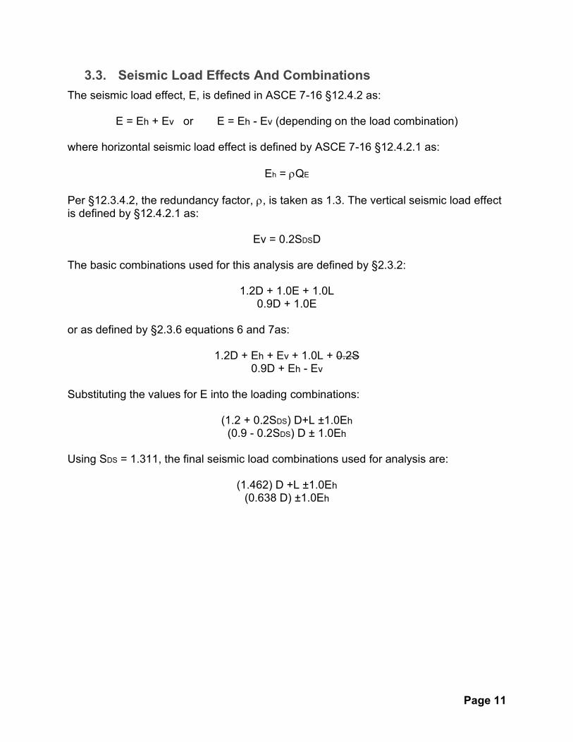
Values for c for the load cases in N-S direction and the requirement of boundary
elements are summarized in table II.6. It shows that BE are required at edge of the
flanges of the c-shape walls. The dimensions of these boundary elements are defined
using ACI 318-14 chapter 18.10.6.4
Table II.6: Load cases, and the need for boundary element, N-S moment
Similar check for the c values for the load cases in E-W direction shows that BE are not
required, see table II.7.
Load / No. LC 1 LC 2 LC 3 LC 4
Pu 7384 -14767 2146 -20005
Mu,ns 33485 -33151 33724 -32912
Vu,ew 1529 -1480 1564 -1445
δu / hw 0.0066 0.0066 0.0066 0.0066
cMax 23.74 23.74 23.74 23.74
ro required 1.4 0.4 0.8 0.4
ro max 1.4 1.4 1.4 1.4
c [inch] 21.7 16.1 33.1 18.9
Boundary no no yes no
0.1 Lw1 [inch] 14.1 14.1 14.1 14.1
c/2 = 16.55
c-0.1Lw1= 19
L_BE [inch] = Max (c/2, c0.1Lw1) 19 required
Prof. Advice Lw1 / 3 70.5
flanged section 33.1 compressed width 18.10.6.4 (d)
choose L_BE [inch] 30 chosen
b_be [inch] hu/16 hu=16'*12 12 >12 inch ok
hw = [inch] 2064
Lw1 = [inch] 141
hw/Lw1= 14.6

Page 26
Table II.7: Load cases, and the need for boundary element, E-W moment
6.3.1. Transverse Reinforcement Of Boundary Elements
According to ACI 318-14 chapter 18.10.6.2 (b), where special boundary elements are
required by (a), the special boundary element transverse reinforcement shall extend
vertically above and below the critical section at least the greater of ℓw and Mu/4Vu. The
extend of this transverse reinforcement is shown in table II.8 for E-W direction. The
required height is 11.8 ft, choose 12 ft in the first floor (from total height of 16 ft), and over
the whole height of the second floor (height is 12ft).
Table II.8: Extend of transversal rebar in boundary element
The design of shear rebar in boundary elements is achieved in accordance with ACI 318-
14 chapter 18.10.6.4 (e). The chosen rebar diameter could be #3 or #4, #4 has been
chosen to get the same hoops as in the wall. All the requirements of chapter 18.7.5.2
have been checked and met.
Smax is the minimum value of: a 1/3 least dimension of the boundary i.e. 30”/3=10”
b 6db of long. bar i.e. 6*1.27” = 7.62“
c So=4+(14-hx)/3 = 4+(14-4.9*2)/3=5.4” (4”<5.4<6”)
Load / No. LC 1 LC 2 LC 3 LC 4
Pu -3691 -3691 -8930 -8930
Mu,ns 144880 -144880 144880 -144880
Vu,ew 1442 -1442 1442 -1442
δu / hw 0.006 0.006 0.006 0.006
cMax 26.11 58.89 58.89 58.89
ro required 1 0.4 0.4 1
ro max 1 1 1 1
ro used 1.4 1.4 1.4 1.4
C 6 8 17 18
BE required No No No No
Load / No. LC 1 LC 2 LC 3 LC 4
Pu 7384 -14767 2146 -20005
Mu,ns 33485 -33151 33724 -32912
Vu,ew 1529 -1480 1564 -1445
Mu/4Vu [ft] 5.5 5.6 5.4 5.7
Lw1 [ft] 11.8 11.8 11.8 11.8
Max(Lw1,Mu/4Vu) [ft] 11.8 11.8 11.8 11.8
Moment N-S and shear EW
Vu,EW
Vu,EW

Page 27
Amount of transverse rebar is defined by 18.10.6.4 (f)
Choose #4 for transverse rebar,
𝐴𝑠ℎ = 4 ∗ 0.2 = 0.80 𝑖𝑛𝑐ℎ S=5” bc=24.7” Ag=30*30=900 𝑖𝑛𝑐ℎ
Ach=24.7*24.7=610 𝑖𝑛𝑐ℎ fc’=7 ksi fyt=60 ksi
Max{ 0.3 (900
6 0− 1)
7
60= 0.0166 , 0.09
7
60= 0.0105 } = 0.0166
𝐴𝑠ℎ
𝑆 𝑏𝑐=
0.8
𝑆∗ .7= 0.0166 >> 𝑆 =
0.8
0.0 66 ∗ .7= 1.95 𝑖𝑛𝑐ℎ ≅ 2 𝑖𝑛𝑐ℎ
Amount of transverse reinforcement is #4 @ 2” o.c.
Figure II.14 Drafting Boundary element, reinforcements and spacings
6.4. Coupling Beams
Designing the coupling beams is achieved according to ACI 318-14 chapter 18.10.7.
Calculation is done according to chapter 18.10.7.4 (a):

Page 28
𝐴𝑣𝑑 =𝑉𝑛
2 𝑓𝑦 sin 𝛼
Max Vu = 610 kips, given from ETABS see chapter 4.4 in this report.
𝑉𝑛 = Vu/Φ = 610 / 0.85 = 718 kips, chapter 21.2.4.3
𝛼 = 𝑎𝑟𝑐𝑡𝑔 −5.5𝑥
8 = 20 𝑑𝑒𝑔𝑟𝑒𝑒𝑠 see figure II.15
𝐴𝑣𝑑 =7 8
𝑥 60 𝑥 sin 0= 17.49 𝑖𝑛𝑐ℎ use 12 # 11 db=1.41 inch
𝐴𝑣𝑑,𝑝𝑟𝑜𝑣𝑖𝑑𝑒𝑑 = 12 1.56 = 18.72 𝑖𝑛𝑐ℎ > 17.49 𝑖𝑛𝑐ℎ ok.
Figure II.15 – Calculating α in the equation 18.10.7.4 of ACI 318-14
Embedding length is calculated according to 18.10.7.4 (b) from 25.4 as follows:

Page 29
Horizontal length is 49” x cos 20 = 46” choose 50”
Figure II.16 Drafting coupling beam, reinforcements and spacings
The design of shear rebar in coupling beams is achieved in accordance with ACI 318-14
chapter 18.7.5.2 have been checked and met.
Smax is the minimum value of: a 1/3 least dimension of the boundary i.e. 30”/3=10”
b 6db of long. bar i.e. 6*1.41” = 8.46“
c So=4+(14-hx)/3 = 4+(14-5.7*2)/3=4.86” (4”<5.4<6”)
18.10.2.3 development length
(a) extend long. reinf. beyond flexure at least 0.8 Lw=0.8*
Lw1 = [inch] 141
0.8 Lw1 = 113
(b) development length calculated from 25.4.2.4 as
fy [psi] 60000
fc' [psi] 7000
lamda 1
psi_t 1.3
psi_e 1
psi_s 1
cb 2.7
Ktr 2.816 Atr=4*0.44 1.76
(cb+Ktr)/db= 2.5 (cb+Ktr)/db= 3.91
db 1.41 < 2.5 2.5
Ld [inch] 39
1.25 fy 18.10.2.3 (b) Ld [inch] 49

Page 30
Amount of transverse rebar is defined by 18.10.6.4 (f)
𝑨𝒔𝒉 horizontal:
2 hoops #6 (4 legs)
𝐴𝑠ℎ = 4 ∗ 0.44 = 1.76 𝑖𝑛𝑐ℎ S=5” bc=30-2.7*2=24.6” Ag=30*42=1260 𝑖𝑛𝑐ℎ
Ach=(30-2.7*2)*(42-2.7*2)=900 𝑖𝑛𝑐ℎ fc’=7 ksi fyt=60 ksi
Max{ 0.3 ( 60
900− 1)
7
60= 0.014 , 0.09
7
60= 0.0105 } = 0.014
𝐴𝑠ℎ
𝑆 𝑏𝑐=
.76
𝑆∗ .6= 0.014 > > 𝑆 =
.76
0.0 ∗ .6= 5.11 𝑖𝑛𝑐ℎ
Use 2 hoops (4 legs) # 6 @ 5” o.c.
Smax should be also min (6”, 6 db=6x1.41=8.46)=6” > 5” ok.
𝑨𝒔𝒉 Vertival
two big hoops #6 and 2 small hoops #4
𝐴𝑠ℎ = 4 ∗ 0.44 + 4 ∗ 0.2 = 2.56 𝑖𝑛𝑐ℎ bc=42-2.7*2=36.6” Ag=30*42=1260 𝑖𝑛𝑐ℎ
Ach=(30-2.7*2)*(42-2.7*2)=900 𝑖𝑛𝑐ℎ fc’=7 ksi fyt=60 ksi
Max{ 0.3 ( 60
900− 1)
7
60= 0.014 , 0.09
7
60= 0.0105 } = 0.014
𝐴𝑠ℎ
𝑆 𝑏𝑐=
.56
𝑆∗ .6= 0.014 > > 𝑆 =
.56
0.0 ∗ 6.6= 5.00 𝑖𝑛𝑐ℎ
Use 2 # 6 @ 5” o.c. and 2 # 4 @ 5” o.c.
Smax should be also min (6”, 6 db=6x1.41=8.46)=6” > 5” ok.
7. Detailing
See attachement

Page 31
PART III: Site Response Spectra and Input Ground Motions
8. Performance Levels
The building should be verified for seismic response for two performance levels:
a) Fully operational at earthquake intensities corresponding to 69% in 50 years of
exposure (resulting in a return period of 43 years), and
b) Near collapse at earthquake intensities corresponding to 2% in 50 years of
exposure (resulting in a return period of 2,475 years).
In this report, the recorded ground motion of M7.3 Landers Earthquake of 28 June 1992
at the Joshua Tree Fire Station site were processed according to the provisions of ASCE
7-16 to design for the 2% in 50 years response.
8.1. ASCE 7-16 Target Spectra
The first step was to find the ASCE 7-16 target spectra. The site class was defined using
the site specific low-strain shear wave velocity V30 presented in Table III.1.

Page 32
Table III.1 Soil Shear Wave Velocities from Specific Site Study
According to ASCE 7-16 chapter 20.4.1, the average velocity was calculated by Equation
1 as 1046.6 ft/s, which corresponds to site class D, stiff soil.
𝑣𝑠 = ∑𝑛
𝑖=1 𝑑𝑖
∑𝑛𝑖=1
𝑑𝑖𝑣𝑠𝑖
(1)
Using the site class and corresponding tables and equations from ASCE 7-16, the
response spectrum parameters were determined and summarized in Table III.2.
𝑆𝑠 𝑆 𝐹𝑎 𝐹𝑣 𝑆𝑀𝑆 𝑆𝑀 𝑆𝐷𝑆 𝑆𝐷 𝑇𝐿 Site
class
Seismicity
1.966 g 0.700 𝑔 1.0 1.7 1.970 𝑔 1.190 𝑔 1.311 𝑔 0.793 𝑔 8 s D high
Table III.2 – ASCE 7-16 Acceleration Response Spectrum Parameters
According to ASCE 7-16, chapter 11.4.6, the pseudo-acceleration elastic design
spectrum for the risk-targeted 𝑀𝑆𝐸𝑅 is simplified to the piecewise relationship shown in
Figure III.1.

Page 33
Figure III.1 ASCE 7-16 Design Response Spectrum
1. For periods less than or equal to 𝑇0 :
𝑆𝑎 = 0.6𝑆𝑀𝑆
𝑇0𝑇 + 0.4𝑆𝑀𝑆
2. For periods greater than 𝑇0 and less than or equal to 𝑇𝑆 :
𝑆𝑎 = 𝑆𝑀𝑆
3. For periods greater than 𝑇𝑆 and less than or equal to 𝑇𝐿 :
𝑆𝑎 =𝑆𝑀
𝑇
4. For periods greater than 𝑇𝐿 :
𝑆𝑎 =𝑆𝑀 𝑇𝐿
𝑇
Where:
𝑇0 = 0.2𝑆𝑀
𝑆𝐷𝑆= 0.1210
𝑇𝑆 =𝑆𝑀
𝑆𝐷𝑆= 0.6049
Note that the 𝑀𝑆𝐸𝑅 parameters (𝑆𝑀𝑆, 𝑆𝑀 ) are used in the relationships above instead of
the Design Earthquake (DE) parameters (𝑆𝐷𝑆, 𝑆𝐷 ). The resulting response spectrum for
2% in 50 years is shown in Figure III.2.

Page 34
Figure III.2 Target Acceleration Response Spectrum, 2% in 50 years
8.2. Site Response Spectra
8.2.1. Ground Motion Conditioning
The Ground motions representing 2% in 50 years for M7.3 Landers Earthquake of 28
June 1992 at the Joshua Tree Fire Station site can be seen below in Figure III.3 for the x
direction and Figure III.4 for the y direction.

Page 35
Figure III.3 Ground Acceleration for Joshua Tree in X-direction
Figure III.4 Ground Acceleration for Joshua Tree in Y-direction
WAVEGEN is a tool that modifies the input/raw ground motion by adding wavelets into
raw ground motion. It requires acceleration data and target spectrum as an input.
WAVEGEN adds sine/cosine (harmonic) wavelets to raw acceleration data in order to
match with target spectrum and gives “compatible.out” file as an output. This
“compatible.out” file is to be used as conditioned ground motion for obtaining response
spectra oriented between 0 to 180 degrees. Besides, the above two files WAVEGEN
requires damping ratio as an input.

Page 36
Once the Ground motions were conditioned to the target acceleration, the maximum-
direction (RotD100) could be found. The two orthogonal x and y acceleration time series
were combined together using Equation 2 to find 90 separate acceleration time series
angles of 0𝑜 ≤ 𝜃 < 180𝑜with 𝛥𝜃 = 2𝑜.
𝑎𝑅𝑂𝑇(𝑡; 𝜃) = 𝑎 (𝑡)𝑐𝑜𝑠(𝜃) + 𝑎 (𝑡)𝑠𝑖𝑛(𝜃) (2)
The pseudo acceleration spectra was then found for each of the angles using Newmark's
Integration Method with 𝛾 = 0.5 and 𝛽 = 0.25 (Constant Average Acceleration Method) to
find and plot the maximum of pseudo acceleration time histories for each period. It can
be seen in Figure III.5, plotted with the ASCE target spectra.
Figure III.5 Cumulative Response from 0 to 180 degrees
The envelope of all 90 directions is RotD100 and it is shown plotted in Figure III.6 with
the target spectrum and 90% of the target spectrum.

Page 37
Figure III.6 Envelope of Unscaled Cumulative Response, Unscaled RotD100
8.2.2. Amplitude Scaling
Once RotD100 was obtained for the Joshua Tree data, it needed to have its amplitude
scaled down according to ASCE 7-16 16.2.3.2 so that it was either equal to or above the
90% target response spectra. The period range for scaling is defined in ASCE 7-16
16.2.3.1 as:
𝑚𝑖𝑛 (𝑇90, 0.2 ∗ 𝑇 ) ≥ 𝑇 ≤ 2 ∗ 𝑇
Where 𝑇 is the largest first translational mode period, 𝑇 is the smallest first translational
mode period, and 𝑇90 is the boundary period including 90% of the mass participation.
This range was thus calculated as:
0.125 𝑠 ≥ 𝑇 ≤ 2.8 𝑠
Within this period scaling range, a scaling factor of 0.9585 was required to scale RotD100
down to rest on the 90% target spectra as seen in Figure III.7.

Page 38
Figure III.7 Envelope of Scaled Cumulative Response, Scaled RotD100
8.2.3. Pseudo Acceleration and Displacement Response Spectra
The scaling factor of 0.9585 was then applied to the Joshua Tree x and y conditional
ground motion accelerations. The pseudo acceleration response spectra and
displacement response spectra for these scaled motions were plotted with the target
spectra as seen in Figures III.8 and III.9. Comparing the scaled acceleration and
displacement responses with the target, it was observed that they are very similar and
essentially right on top of one other.

Page 39
Figure III.8 Target and Scaled Conditioned Acceleration Response Spectra
Figure III.9 Target and Scaled Conditioned Displacement Response Spectra

Page 40
PART IV: Non-Linear Model
9. Variant 1 of Non-Linear Model
In this part of the project, the importance of uncertainty that arises from the use of a
damping model in non-linear time-history analysis is to be understood. The non-linear
time history analysis is carried out in ETABS. The model provided in ETABS has core
walls modeled as frame elements with distributed plasticity (Displacement-based
formulations) and sections discretized with concrete and steel fibers. The coupling beams
are modeled using diagonal nonlinear truss elements. This idealization of model is more
representative of the actual behavior of a coupling beam than models based on springs
commonly used in practice.
9.1. Complete Core Wall Design for Combined Axial-Flexure
In this section, the design is done partially separate for Level 1 to 5 and for Level 6 to 14.
For level 1 to 5, the design is kept exactly similar to the design of core wall in Part I except
for the design of coupling beams. For level 6 to 14, identical longitudinal and transverse
reinforcement are redesigned for maximum load values. The design of coupling beams
is further divided into three sections namely, level 1 to 4, level 5 to 8 and level 9 to 14.
Coupling beams for level 1 to 4 are designed with maximum load coming on that levels
and likewise it is done for level 5 to 8 and level 9 to 14.
After identifying critical load combinations for Level 6 to 14 from ETABS model, values
are plotted on P-M interaction diagrams for E-W and N-S. From the diagram, the values
of minimum reinforcement ratio is coming out to be 0.80%. Critical Load combinations
acting on the walls are tabulated below in Table IV.1 and Table IV.2 for Core Wall AB and
CD.
Core Wall AB
Load Combo Pu (kips) Mu_NS (k-ft) Mu_EW (k-ft)
1 1.5D+L+E_EW 709.1 13816.2 0
2 0.64D+E_EW 3755.5 13727.3 0
3 1.5D+L+E_NS -5407.7 0 73458.5
4 0.64D+E_NS -2227.7 0 73458.5
Table IV.1 Critical Load Combination for Core Wall AB

Page 41
Core Wall CD
LC Pu (kips) Mu_NS (k-ft) Mu_EW (k-ft)
1 1.5D+L+E_EW -11287.6 -13816.2 0
2 0.64D+E_EW -8107.7 -13727.3 0
3 1.5D+L+E_NS -5407.7 0 -73458.5
4 0.64D+E_NS -2227.7 0 -73458.5
Table IV.2 Critical Load Combination for Core Wall CD
The values of Axial Load and Moment combinations are plotted on P-M interaction
diagrams of EW and NS direction respectively. P-M Interaction diagrams for E-W and
N-S direction are shown below in Figure IV.1 and Figure IV.2.
Figure IV.1 P-M Interaction Diagram in E-W Direction

Page 42
Figure IV.2 P-M Interaction diagram for N-S direction
Design of Longitudinal and Transverse Reinforcement
Design of Longitudinal reinforcement is carried out using obtained reinforcement ratio of
0.8 % from P-M Interaction diagram and gross area of the section of wall. From the
calculation, #8 bars at 7 in. OC are to be provided in 2 curtains. Similarly, transverse
reinforcement is designed for maximum shear demand in E-W and N-S direction
respectively. From the calculation, it is found that minimum reinforcement of 0.25 % is
sufficient. Transverse reinforcement of #4 bars at 6 in. OC in 4 curtains are provided in
E-W direction and #4 bars at 6 in. OC in 2 curtains are provided in N-S direction.
Detailed calculation is shown in Appendix B.
Design of Coupling Beams
Design of coupling beams are done for 3 different categories based on groups of
coupling beams, i.e, Level 1 to 4, Level 5 to 8 and Level 9 to 14. It was assigned to find
the maximum coupling beam shear on each of the floors and design the coupling beams

Page 43
accordingly. The maximum shears for each of the floor categories can be seen in Table
IV.3.
Table IV.3 Coupling Beam Shear Forces
Design Summary
Design detail summary of shear wall and coupling beams based on calculations similar
to that done in Part II shown in Table IV.4.
Design Detail Summary of Core Wall
Shear Wall
Longitudinal Reinforcement #11 bars @ 7 in. (Level 1 to 5) #8 bars @ 7 in. (Level 6 to 14)
Transverse Reinforcement #4 bars @ 5 in. (Level 1 to 5) #4 bars @ 6 in. (Level 6 to 14)
Coupling Beams
Longitudinal Reinforcement 12 #11 bars in 3 layers (Level 1 to 4) 12 #11 bars in 3 layers(Level 5 to 8) 8 #11 bars in 2 layers(Level 9 to 14)
Transverse Reinforcement 5 legs vs 6 legs with 2 bundled #4 bars each leg (Level 1 to 4)
4 legs vs 6 legs with 2 bundled #4 bars each leg (Level 5 to 8)
4 legs vs 6 legs with 2 bundled #4 bars each leg (Level 9 to 14)
Table IV.4 Design Summary
Detailed Drawings
Detailed Drawings are attached in Appendix A.
9.2. Modal Analysis
Modal Analysis is the study of dynamic properties of the structures under consideration in
frequency domain. Modal analysis is also of great importance to study about resonating behavior
of structure. It identifies the periods at which the structure/system may resonate at its natural

Page 44
frequency. It also talks about the various modes in which structure/system may vibrate under the
given earthquake conditions which eventually helps in identifying possible zones of damage.
Modal Response in X - Direction
Figure IV.3 Modal Response in X - Direction
The modal properties of the structure in X-direction for Mode 1, Mode 2 and Mode 3 are
tabulated below in Table IV.5, Table IV.6 and Table IV.7 respectively.

Page 45
Table IV.5 Modal Properties of Structure in X-Direction for Mode 1
Table IV.6 Modal Properties of Structure in X-Direction for Mode 2
Table IV.7 Modal Properties of Structure in X-Direction for Mode 3

Page 46
Y - Direction
Figure IV.4 Modal Response in Y - Direction
The modal properties of the structure in Y-direction for Mode 1, Mode 2 and Mode 3 are
tabulated below in Table IV.8, Table IV.9 and Table IV.10 respectively.
Table IV.8 Modal Properties of Structure in Y-Direction for Mode 1

Page 47
Table IV.9 Modal Properties of Structure in Y-Direction for Mode 2
Table IV.10 Modal Properties of Structure in Y-Direction for Mode 3
Mode Period (seconds)
X-Direction
1 0.952
2 0.266
3 0.128
Y-Direction
1 1.078
2 0.259
3 0.116
Table IV.11 Summary of Period for various modes in X and Y Directions

Page 48
Cumulative Modal Participation Mass Ratio
The plot of cumulative modal mass participation ratio vs. period is plotted for both linear
and non-linear model in X and Y directions. Surprisingly, non-linear model seems to have
lesser period making it stiffer than linear model. This behavior is due to the fact that for
linear model, stiffness modifiers are incorporated for conservative estimates whereas for
nonlinear model full stiffness (uncracked section initially) of the structure is taken into
account.
Figure IV.5 Cumulative Modal Mass Participation vs Period in X-Direction
Figure IV.6 Cumulative Modal Mass Participation vs Period in Y-Direction

Page 49
Besides, it is also observed that upto 60 percent mass of the building take part into first
translational mode, then upto 90 percent mass of the building take part into second
translational mode and approximately 5 percent mass from the remaining 10 percent
mass takes part into third translational mode.
9.3. Influence of the Damping Model on the Nonlinear Dynamic
Response
In this section, the effect of damping model on nonlinear response of a building is
analyzed. Rayleigh (proportional) damping is generally available in all non-linear dynamic
analysis programs. This damping model is convenient as it is a linear combination of the,
usually banded, stiffness and mass matrices. Damping coefficients for this model are
determined by selecting damping ratios for only two modes.
1. Set damping ratio of 2.0% in the first translational mode in the NS direction and in
the first translational mode in EW direction. Plot the damping ratio (Y-axis) from 0
to 25% and the frequency range (X-axis) from 0 to 20 Hz.
2. Set damping ratio of 2.0% in the average frequency of the first translational mode
in the NS direction and the first translational mode in the EW direction, and 5% at
a circular frequency of 125.6 rad/s (f = 20 Hz, T = 0.05s). Plot the damping ratio
(Y-axis) from 0 to 10% and the frequency range (X-axis) from 0 to 20 Hz.
Relation between Damping ratio and modal frequency:
The damping ratio of a structure/system in nth mode is calculated as below:
(1)
The Rayleigh damping coefficients 𝛼 𝑎𝑛𝑑 𝛽are determined from the given damping ratio
for the ith and jth mode respectively. In the matrix form, it can be written as:
(2)
Upon solving the above matrix equation, we can get the values of 𝛼 𝑎𝑛𝑑 𝛽given that both
modes have same damping ratio.
Hence, we can get the equations of 𝛼 𝑎𝑛𝑑 𝛽as follows:

Page 50
(3)
The equations are solved in MATLAB and values obtained are tabulated below in Table
VI.12.
Case 𝛼 (𝑠𝑒𝑐−1) 𝛽 (𝑠𝑒𝑐 )
Case - 1 0.1238 0.0032
Case - 2 0.2184 0.0008
Table IV.12 Values of Coefficients for Case - 1 and Case – 2
Using these two coefficients, values of damping ratio are calculated for a given frequency
range (0 to 20 Hz) by using Equation 1. The plot for both cases is shown below in Figure
IV.7.

Page 51
Figure IV.7 Damping Ratio vs Frequency
The frequency for Mode 1 and Mode 2 in X and Y Direction is tabulated below which is
evident from Table IV.13.
X - Direction Y - Direction
Frequency (Hz) Frequency (Hz)
Mode 1 1.0504 0.9276
Mode 2 3.7594 3.8610
Table IV.13 Modal Frequencies in X and Y Direction

Page 52
The corresponding damping ratio for each mode in each direction is tabulated below in
Table IV.14.
Damping Ratio (𝜁%)
1st Translational Mode 2nd Translational Mode
EW (X Direction)
Case - 1 2.00 4.05
Case - 2 1.91 1.38
NS (Y Direction)
Case - 1 2.00 4.15
Case - 2 2.10 1.39
Table IV.14 Damping Ratio for Mode 1 and Mode 2 in EW and NS Direction
From Table IV.14 it is evident that for both cases 1st Translational Mode has more or less
same damping ratios. However, for 2nd translational mode, Case-1 seems to be
overdamped compared to Case-2.

Page 53
Nonlinear Time History Analysis
In this section, nonlinear time history analysis is performed using MCE conditioned
ground motion pairs of JOSHUA earthquake for cases mentioned above. Integration
scheme used was constant average acceleration with output time step size of T = 0.005
seconds.
Lateral Floor Displacement
Figure IV.8 Relative Lateral Floor Displacement - EW
Figure IV.9 Relative Lateral Floor Displacement - NS

Page 54
Interstory Drift Ratio
Figure IV.10 Interstory Drift Ratio - EW
Figure IV.11 Interstory Drift Ratio - NS

Page 55
Total Floor Acceleration
Figure IV.12 Total Floor Acceleration - EW
Figure IV.13 Total Floor Acceleration - NS

Page 56
Observations on Diagrams
1. Maximum relative displacement is seen in the middle floors 6-8 in EW (X) direction
and the upper stories in NS (Y) direction.
2. Similar trend could be seen in the interstory drift ratio. Minimum / maximum values
are -1.5 inch / 2.0 inches in EW (X) direction, and -2.5 inch / 2.0 inches in NS (Y)
direction.
3. Maximum floor acceleration occurs in the last story in either direction EW (X) and
NS (Y).
4. Maximum and minimum accelerations has almost the same absolute values, in
direction EW (X) it is 1g for case 1 and 1.7g for case 2, in the direction NS (Y) it
is 1.4g for case 1 and 2.2g for case 2. Case 2 shows higher acceleration values in
all stories, in both directions, than case 1.

Page 57
10. Variant 2 of Non-Linear Model
In this part of the project, another ETABS 2018 model is to be used. This model is similar
to the model used in Part III except for the coupling beams. Here, the coupling beams are
modeled using vertical nonlinear link elements (equivalent shear spring model) connected
to rigid elements cantilevering from the walls. The equivalent springs are widely used in
practice, however models based on diagonal nonlinear truss elements (equivalent truss
model) are more representative of the actual behavior of the coupling beams. Your
Professor will discuss both methods in class.
10.1. Influence of the Coupling Beam Model on the Nonlinear
Dynamic Response
In this section, the effect of the model for the coupling beams on the response of a core
wall will be seen. Using the damping Case 2 described in III.4, the nonlinear ETABS
models provided of Part III (equivalent truss model) and Part IV (equivalent shear spring)
will be updated with the flexural reinforcement in the walls and the diagonal reinforcement
in the coupling beams computed in III.2.The two ETABS models will be subjected to the
same MCER scaled ground motion pair.
Equivalent Truss Model
● The beam is modeled as two truss elements located along the centroidal axis of
the diagonal reinforcement in the beam.
● The cross-section of each truss contains the total steel area in the diagonal as well
as an equivalent area of concrete (Ac,eq), determined by matching the stiffness of
the model to the un-cracked section of the beam.
● Additionally, the capacity in tension of the concrete fibers must be adjusted to
match the actual shear stress at the onset of cracking (Vcr) .
According to Timoshenko beam theory, the stiffness of a deep beam can be computed
as follows:

Page 58
The equivalent truss model under the same cracking force:
From equilibrium in the transverse direction of the equivalent truss model, the equivalent
concrete area is calculated by:
Equivalent Shear Spring Model
In this model the coupling beam is modeled using two rigid elements connected by a
spring representing the shear in the transverse direction.

Page 59
This model is constituted by a single material model, representing the steel reinforcement,
and does not capture the initial stiffness and onset of cracking of the beam section.
The properties of the spring element are determined by matching the initial yield of
reinforcement in the beam (Δy, Vy). While in the truss model the onset of yield state is not
computed explicitly, the shear spring formulation requires explicit values for Δy and Vy.

Page 60
To model the shear spring using a fiber section of steel with a unit area, use the following
properties for the material model (e.g. Steel02)
Figure IV.14 and Figure IV.15 show the negative and positive envelopes in the EW
direction for relative lateral floor displacement and interstory drift ratio of the truss and
spring models respectively:
Figure IV.14 Relative Lateral Floor Displacement, E-W Direction

Page 61
Figure IV.15 Interstory Drift Ratio, E-W Direction
From the above graphs, both the Truss and Spring models appear to have similar relative
displacements and drift ratios. It can be seen in Figure IV.14, especially in the negative
drift where the core wall reinforcement changes at floor 9 and the building drifts more
drastically between floors 9 and 14.
Figure IV.16 shows graph of the the core wall shear force (total shear force).

Page 62
Figure IV.16 Core Wall Total Shear Force - E-W direction
From Figure IV.16, it is evident that the truss and spring models provide similar total shear
force results until you get to the bottom of the building, where the Truss model shows
larger shears. This is because the Truss model, unlike the spring model, is able to show
the lengthening in the coupling beams. The coupling beams are able to expand at the
top of the building, but once you get to the base, the walls are much stiffer closer to the
stiff foundation and unable to spread apart, thus causing an increase in the shear force
and a redistribution between the two walls that will be seen in later figures.
Figure IV.17 and Figure IV.18 show the hysteretic responses given by truss and spring
models for the south side coupling beams in Story 1 and Story 4 respectively:

Page 63
Figure IV.17 Hysteretic Responses Given by Truss Model and Spring Model in
Story 1
Figure IV.18 Hysteretic Responses Given by Truss Model and Spring Model in
Story 4
As seen from the above plots, the bauschinger effect is more clear in the truss model
which is more precise, however the spring model is more often used in industry for

Page 64
simplicity. In Story 1, the maximum shear force in the truss model is ±1500kips (more
precise value), while in the spring model it is ±900kips (approximate value). Linear
hysteresis response of the spring model suggests that one spring can not predict the
actual behavior of the coupling beam. Energy Dissipation is more or less linearly confined
for Story 4 compared to Story 1 in which Truss Model simulates non-linear behavior by
incorporating yielding and then moving into nonlinear range. At story 1, the truss model
provides a better estimation of energy dissipation compared to the spring model.
The following Figure IV.19 and Figure IV.20 show the envelope of the c-shaped wall shear
forces in the EW and NS directions for the truss and spring models. Shear forces that
were used for the design (linear analysis) are shown with them for comparison:
Figure IV.19 C-shaped Wall Enveloped Shear - EW

Page 65
Figure IV.20 C-shaped Wall Enveloped Shear - NS
The EW direction is the direction of the coupling beams, thus in Figure IV.19, the Truss
model shows an extreme jump in enveloped shear at the base where almost all of the
base shear is going into one of the C-shaped walls due to the redistribution in shear at
the stiff base of the building as discussed previously. The spring model is unable to
represent the lengthening in the beams, or the redistribution of shear to the walls, and
thus shows a much lower enveloped shear at the base.
The NS direction is perpendicular to the coupling beams and the walls have no
redistribution of the shear force at the base, thus in Figure IV.20, the truss and spring
models show very similar results.
In both figures, it is clear that the design shear from linear analysis used for the core wall
design is far under designing the walls when you look at the nonlinear results.
The following Figures IV.21 to IV.24 show the shear forces in each of the c-shaped walls
in the EW direction for the truss and spring models, at both the positive peak base shear
force and the negative base shear force, plotted with both the shear force from the linear
model and the design shear forces chosen for the floor sections:

Page 66
Figure IV.21 Shear Force Distribution at Positive Peak Base Shear - Truss Model
Figure IV.22 - Shear Force Distribution at Negative Peak Base Shear - Truss Model

Page 67
Figure IV.23 - Shear Force Distribution at Positive Peak Base Shear - Spring
Model
Figure IV.24 - Shear Force Distribution at Negative Peak Shear - Spring Model

Page 68
Figures IV.21 and IV.22 for the truss model shows that the shear force in walls C1 and
C2 are the same until the base where there is a huge evident redistribution of shear into
the leading wall and far less shear in the trailing wall. This behavior is not seen in the
Spring model shown in Figure IV.23 and IV.24 where the shear stays almost the same
across the height of the core wall.
The Design linear shear forces are again seen to be unconservative for the bottom 4
floors and closer yet conservative for the top floors. There is an evident discrepancy
between the linear and nonlinear results.
Figures IV.23 and IV.24 for the spring model doesn't show the difference seen in the truss
model, this model can’t capture the redistribution of shear forces the truss model can
show.
Similar to the truss model, the Design linear shear forces are seen to be unconservative
for the bottom 4 floors and closer yet conservative for the top floors. There is an evident
discrepancy between the linear and nonlinear results.
10.2. Estimated Roof Displacement
To gain confidence in the ETABS model results, the roof displacement from the nonlinear
model in Part III will be compared to displacements corresponding to MCER level
calculated from the following Equation:
ΔN = Estimated roof displacement in the direction considered (NS or EW).
Γ*1 = Modal contribution factor for mode 1 in the direction considered (NS or EW).
Sd = spectral displacement from the response spectrum (ζ=5%) at period Tp
Tp = predominant period which is assumed to range from 1.5T1 to 1.7T1
T1 = period of the first mode in the direction considered (NS or EW).
Ꞵ = 0.8 from Table 17.5-1 of ASCE 7-16 considering ζ=2%
CR = displacement coefficient Sdi/Sd, assumed as 1 (equal displacement)
Table IV.15 Estimated vs Model Roof Displacement

Page 69
The predominant period range and results can be seen in Table IV.15 above. The EW
ETABS roof displacement of 23 in. is in the estimated displacement range of 22.81 in. -
31.25 in, while the the NS ETABS roof displacement of 26.9 in. is just outside the
estimated displacement range of 31.33 in. to 35.57 in. The NS displacement is close
enough to the range to put it in the probability distribution of the estimation and the results
are still able to provide a level of confidence in the results.

Page 70
PART V: Design Verification
11. General
Part V of the project is intended to verify the Fully Operational and Life Safety
performance objectives of the core wall designed previously. Non-linear time-history
analysis was used to determine usage ratios. Usage ratios are defined as the demand
obtained from the nonlinear analysis over the damage limit state for a specific parameter.
The damage limit states are listed in V.2. At this stage it was assumed that the shear
reinforcement was sufficient.
11.1. Performance Objectives
1. Fully operational was checked against ground motions representing the seismic
hazard with 69% probability of exceedance in 50 years of exposure (i.e. a return
period Tp = -E / ln (1 – PE) = 43 years, where the exposure time is E = 50 years
and the probability of exceedance is PE = 69%):
- Gypsum board partition walls: Interstory drift ratio shall not exceed 0.6%.
- Strain in any longitudinal core wall reinforcing bar and in the diagonal
reinforcement in the coupling beams shall not exceed 1% (i.e. damage limit
state sii, residual cracks likely to remain large).
- Compressive strain at the extreme corner fibers at each wall at base shall
not be less than -0.4% (i.e. damage limit state cii, onset of concrete cover
spalling).
2. Life Safety was checked against ground motions representing the seismic hazard
with 2% probability of exceedance in 50 years of exposure (i.e. a return period Tp
= -E / ln (1 – PE) = 2475 years, where the exposure time is E = 50 years and the
probability of exceedance is PE = 2%):
- Strain amplitude (maximum tensile strain minus the minimum compressive
strain) in any longitudinal core wall reinforcing bar and in the diagonal
reinforcement in the coupling beams shall not exceed (14 – 1.33Sh/db)/100
and cc <=-0.004 ,this is the reinforcement damage limit-state siv, longitudinal
bar fracture.
- Compressive strains at the core wall base shall not be less than -0.4%. Shall
not exceed the crushing strain.
- Maximum tensile strain in the core wall longitudinal reinforcement away
from the plastic hinge region at the wall base shall not exceed 1% (i.e.
Page 71
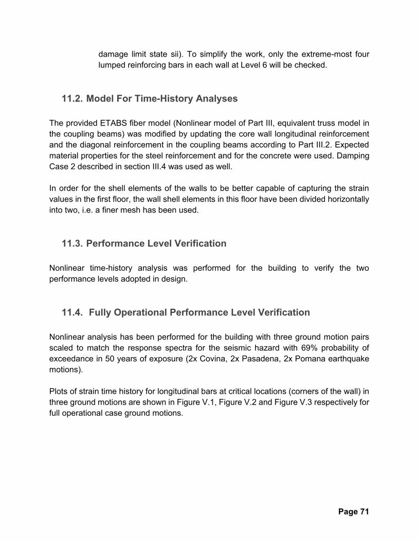
damage limit state sii). To simplify the work, only the extreme-most four
lumped reinforcing bars in each wall at Level 6 will be checked.
11.2. Model For Time-History Analyses
The provided ETABS fiber model (Nonlinear model of Part III, equivalent truss model in
the coupling beams) was modified by updating the core wall longitudinal reinforcement
and the diagonal reinforcement in the coupling beams according to Part III.2. Expected
material properties for the steel reinforcement and for the concrete were used. Damping
Case 2 described in section III.4 was used as well.
In order for the shell elements of the walls to be better capable of capturing the strain
values in the first floor, the wall shell elements in this floor have been divided horizontally
into two, i.e. a finer mesh has been used.
11.3. Performance Level Verification
Nonlinear time-history analysis was performed for the building to verify the two
performance levels adopted in design.
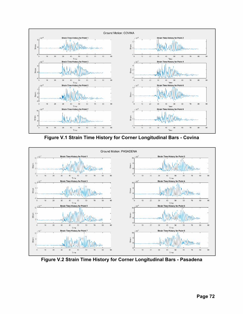
11.4. Fully Operational Performance Level Verification
Nonlinear analysis has been performed for the building with three ground motion pairs
scaled to match the response spectra for the seismic hazard with 69% probability of
exceedance in 50 years of exposure (2x Covina, 2x Pasadena, 2x Pomana earthquake
motions).
Plots of strain time history for longitudinal bars at critical locations (corners of the wall) in
three ground motions are shown in Figure V.1, Figure V.2 and Figure V.3 respectively for
full operational case ground motions.
Page 72
Figure V.1 Strain Time History for Corner Longitudinal Bars - Covina
Figure V.2 Strain Time History for Corner Longitudinal Bars - Pasadena

Page 73
Figure V.3 Strain Time History for Corner Longitudinal Bars - Pomona
Figure V.4 Location of Critical Points on Core Wall
Critical points of the core wall are labeled from 1 to 8 and can be seen on Figure V.4
Table V.1 shows the strain values and usage ratios for Sii (i.e. the maximum tensile strain
for each lumped reinforcement and for each ground motion over a limit of 0.01). Table
V.2 shows the usage ratios for the unconfined concrete (limit state Cii, onset of concrete
cover spalling) at the eight critical points at the core wall base.
3 4 7 8
1 2 5 6
Points 1,3,5,7 under compression Points 2,4,6,8 under tension

Page 74
Point Strain Values Usage Ratio, Sii
Covina (10-4) Pasadena Pomona Covina Pasadena Pomona
1 5.28 0.0010 0.0010 0.0528 0.1015 0.1035
2 6.77 0.00098 0.0011 0.0677 0.0980 0.1127
3 7.21 0.0010 0.00096 0.0721 0.1032 0.0962
4 5.26 0.0094 0.00084 0.0526 0.0940 0.0841
5 5.24 0.00101 0.00088 0.0524 0.1016 0.0886
6 5.56 0.00104 0.00098 0.0556 0.1039 0.0987
7 7.92 0.00108 0.00106 0.0792 0.1086 0.1060
8 5.77 0.00104 0.00089 0.0577 0.1045 0.089
Max 0.792 0.1086 0.1127
Table V.1 Usage Ratios for Longitudinal Bars at Critical Locations, Sii
Point
Strain Values Usage Ratio, Cii
Covina(10-4) Pasadena(10-4) Pomona(10-4) Covina Pasadena Pomona
1 -3.42 -5.25 -3.71 0.0855 0.1312 0.0928
2 -3.27 -3.10 -3.56 0.0817 0.0775 0.0890
3 -3.92 -5.59 -5.08 0.0980 0.1398 0.1270
4 -2.44 -3.38 -3.14 0.0610 0.0845 0.0785
5 -2.59 -3.34 -3.17 0.0648 0.0860 0.0793
6 -4.58 -5.72 -4.73 0.1145 0.1430 0.1183
7 -2.6 -3.09 -3.52 0.065 0.0773 0.0880
8 -3.41 -5.31 -4.16 0.0852 0.1328 0.1040
Max 0.1145 0.1430 0.1270
Table V.2 Usage Ratio for Unconfined Concrete at Critical Locations, Cii
Page 75
As shown in Table V.1 and Table V.2, Usage ratio for longitudinal reinforcement and
unconfined concrete at critical locations (corners of core wall) were calculated
respectively. Upon comparison with limit values of strain tension (0.01) and in
compression (-0.004), it was found that extreme corners of the wall remain safe under
ground motions provided for full occupancy condition. For longitudinal reinforcement,
considering maximum tensile strain, maximum usage ratio came out to be 0.1127 at point
2, whereas in the case of unconfined concrete, the maximum usage ratio came out to be
0.1430 at point 6.
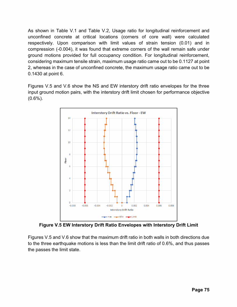
Figures V.5 and V.6 show the NS and EW interstory drift ratio envelopes for the three
input ground motion pairs, with the interstory drift limit chosen for performance objective
(0.6%).
Figure V.5 EW Interstory Drift Ratio Envelopes with Interstory Drift Limit
Figures V.5 and V.6 show that the maximum drift ratio in both walls in both directions due
to the three earthquake motions is less than the limit drift ratio of 0.6%, and thus passes
the passes the limit state.

Page 76
Figure V.6 NS Interstory Drift Ratio Envelopes with Interstory Drift Limit
Figures V.7 and Figure V.8 show the usage ratios for each level ( the envelope of drift
ratio at each level divided by the damage limit drift ratio stated in V.1.1). They are plotted
with the usage ratio limit of one.
Figure V.7 EW Usage Ratios of Interstory Drift Ratio Envelopes

Page 77
Figure V.8 NS Usage Ratios of Interstory Drift Ratio Envelopes
In Figure V.7 and Figure V.8 the maximum usage ratio in EW directions is 0.5 and 0.65
in NS direction,both less than 1. Thus, the usage ratio of interstory drift ratio meets the
criteria.
Table V.3 below shows the usage ratios for the damage limit state sii (residual cracks
likely to remain large) in coupling beams. In this table the tensile strains in the outermost
longitudinal bar are compared with the limit, 𝜀𝑠 = 1%.
Story Strain (Max. Tensile) Usage Ratio
Covina Pasadena Pomona Covina Pasadena Pomona
14 0.00018 0.00014 0.00006 0.0182 0.0136 0.0063
13 0.00050 0.00045 0.00026 0.0496 0.0449 0.0263
12 0.00071 0.00073 0.00051 0.0710 0.0731 0.0513
11 0.00082 0.00094 0.00067 0.0818 0.0935 0.0667
10 0.00089 0.00107 0.00077 0.0888 0.1072 0.0770
9 0.00092 0.00117 0.00084 0.0921 0.1168 0.0835

Page 78
8 0.00089 0.00116 0.00089 0.0891 0.1157 0.0891
7 0.00087 0.00118 0.00092 0.0874 0.1177 0.0920
6 0.00084 0.00119 0.00099 0.0842 0.1193 0.0988
5 0.00093 0.00119 0.00104 0.0931 0.1188 0.1039
4 0.00100 0.00119 0.00107 0.0999 0.1193 0.1066
3 0.00100 0.00113 0.00105 0.0997 0.1129 0.1047
2 0.00092 0.00101 0.00099 0.0924 0.1006 0.0994
1 0.00081 0.00085 0.00080 0.0812 0.0847 0.0802
Max 0.0999 0.1193 0.1066
Table V.3 Usage Ratio for Damage Limit State in Coupling Beams, Sii
From Table V.3, the maximum usage ratio is 0.1193 (11.9%) at story 6. Thus, the
structure passes the Sii limit state criteria.
11.5. Life Safety Performance Level Verification
Nonlinear analysis was performed on the building model with the same three ground
motion pairs scaled to match the response spectra for the seismic hazard with 2%
probability of exceedance in 50 years of exposure.
Strain time histories were taken from the ETABS model from three points on each wall
(P, Q, and R), whose location can be seen in Figure V.9. With the strain as the Z value
and the X and Y values being taken from the defined origin (Figure V.9), vectors were
formed from these points and used to form planes for each wall separately at each time
step. These planes were used to calculate the maximum tensile strain and minimum
compressive strain contours along the core walls as seen in Figures V.10 and Figure
V.11. The strain amplitude was also calculated as maximum tensile strain minus the
minimum compressive strain and its strain contour is seen in Figure V.12.

Page 79
Figure V.9 Vectors with Center Points on the Core Wall
The strain amplitude was compared to the Siii limit state for the onset of long bar
buckling:
𝜀𝑠−𝜀𝑐𝑐 ≥ 0−
𝑆ℎ
𝑑𝑏
00 = 0.064
and was also compared to the Ciii limit state for deep concrete cover spalling:
𝜀𝑐𝑐 ≥ −0.004
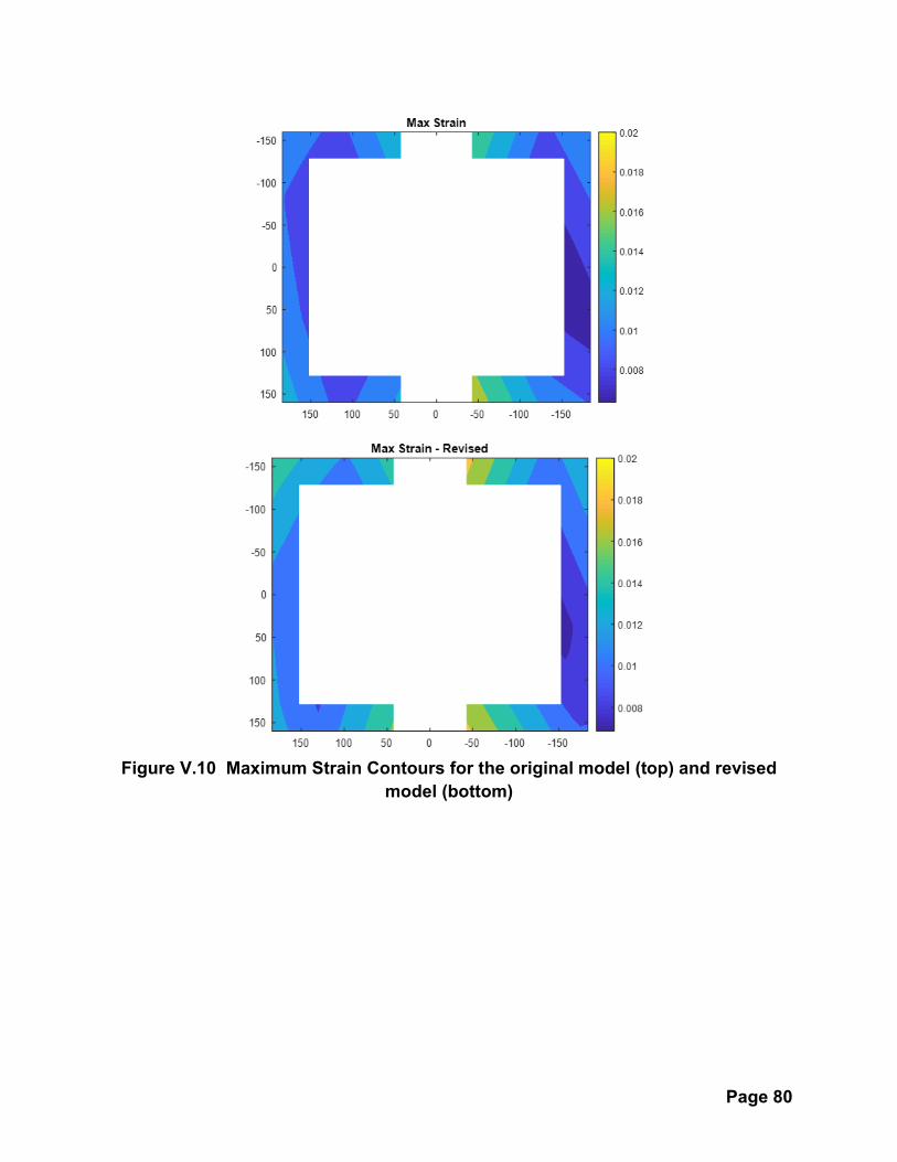
While the entire core wall met the criteria for limit state Siii, there was an edge of the wall
that did not meet the Ciii limit state and would thus require boundary elements, as seen
in Figure 13. However, the strains at the extreme corners of the 6th floor showed that the
steel was yielding and forming a plastic hinge ( discussed in more detail below), and it
was decided that the best course of action would be to extend the 1.4% longitudinal
reinforcement up to the 8th floor to mitigate the mid building plastic hinging. The model
was changed and rerun with the new reinforcement, new strains were taken, and the new
contour plots can be seen on the bottom of Figures 10, 11, and 12. This change caused
more of the edges of the core walls to require reinforcement as seen in the revised Figure
13. The zone that did not pass the Ciii limit state extended a maximum of 20 inches into
the core wall. Since core wall reinforcement was previously detailed to be 24 inches at
every corner based on the linear analysis, it did not need to be revised after the non-linear
analysis.
Q1 Q2
+ Origin
R1 R2
P1 P2
Page 80
Figure V.10 Maximum Strain Contours for the original model (top) and revised
model (bottom)

Page 81
Figure V.11 Minimum Strain Contours for the original model (top) and revised
model (bottom)

Page 82
Figure V.12 Strain Amplitude Contours for the original model (top) and revised
model (bottom)

Page 83
v
Figure V.13: Locations requiring boundary elements (black) for the -0.004
minimum strain limit for the original model (top) and revised model (bottom)

Page 84
Strains were extracted from the extreme fibers of the contours and compared to the limit
state Siv, Bar Fracture, and Civ, Crushing of the confined concrete core. The Siv limit
state for the onset of long bar buckling is shown below:
𝜀𝑠−𝜀𝑐𝑐 ≥ −
4𝑆ℎ
3𝑑𝑏
00= 0.092
The Ciii limit state for deep concrete cover spalling was based on the rectangular cross
section equation and was calculated from the boundary element reinforcement:
𝜀𝑐𝑐 ≥ −(0.004 + 2√𝜌𝑠𝑥𝜌𝑠𝑦)= -0.026
The usage ratios are seen tabulated in Tables V.4 and Table V.5.
Wall C1 Wall C2
Point Strain Usage Ratio Strain Usage Ratio
Top left 0.018 0.220 0.0221 0.270
Top Right 0.0205 0.251 0.0152 0.186
Bottom Left 0.0149 0.182 0.0221 0.270
Bottom Right 0.0204 0.249 0.0127 0.155
Table V.4 Usage Ratio for Reinforcement at Wall corners on Level 1, Siv
Wall C1 Wall C2
Point Strain Usage Ratio Strain Usage Ratio
Top left -0.0025 0.098 -0.0032 0.125
Top Right -0.0053 0.208 -0.0014 0.055
Bottom Left -0.0018 0.071 -0.0036 0.141
Bottom Right -0.004 0.157 0.0025 0.098
Table V.5 Usage Ratio for Reinforcement at Wall corners on Level 1, Civ

Page 85
From Table V.4 and V.5 it can be seen that the core walls met the Civ and Siv criteria and
there was no bar fracture or crushing of the confined concrete core.
Usage Ratio for all eight-lumpred reinforcement at the wall corners at Level 6 were also
obtained for two reinforcement scenarios and comparative study is presented here.
In the first case, the model was provided with 1.4% longitudinal reinforcement in stories
1 to 5 and 0.8% longitudinal reinforcement between story 6 to 14. Usage ratios for this
case are calculated at level 6. In the second case, the model was provided with 1.4%
longitudinal reinforcement farther up, between story 1 to 8 and usage ratios for level 6
were again calculated. This comparison gives rise to an idea that differentiates
performance based design to conventional seismic design. Usage Ratios for both cases
are shown below in Table V.6.
Point Usage Ratio, 0.8% Long. R/F Usage Ratio, 1.4% Long. R/F
Castaico Joshua Yermo Castaico Joshua Yermo
1 1.3864 0.9109 1.0524 0.5303 0.2377 0.2700
2 1.2607 0.8905 0.9573 0.5194 0.2090 0.3098
3 0.5347 1.4576 0.6989 0.2051 0.2615 0.2004
4 0.4732 1.2828 0.7590 0.2338 0.2807 0.1691
5 0.7364 1.0174 0.9858 0.2295 0.2161 0.3018
6 0.6073 1.1792 1.0879 0.2020 0.2285 0.3577
7 0.6913 0.9360 1.0064 0.2107 0.3343 0.1986
8 0.7577 1.0554 1.2165 0.2561 0.3342 0.2295
Max 1.3864 1.4576 1.2165 0.5303 0.3343 0.3577
Table V.6 Usage Ratio for Reinforcement at Wall corners on Level 6, Sii
From Table V.4, it is evident that when incorporating performance based design, the
usage ratio significantly reduces due to provision of higher percentage of longitudinal
reinforcement. When the model is provided with 1.4% longitudinal reinforcement only up
to level 5, plastic hinge forms at level 6, which is evident from tensile strain based usage
ratios greater than 1. These drop by approximately 60% for Castaico, 80% for Joshua
and 70% for Yermo. From this observation one can conclude that the longitudinal

Page 86
reinforcement curtailment should be done in a manner that it allows plastic hinge to form
at base and not at upper levels.
Table V.7 shows usage ratio for damage limit state in coupling beams for the diagonal
reinforcement. It compares the strain value for each ground motion with critical value Siv.
The limit for coupling beam was calculated as 0.082.
Story Strain (Max. Tensile) Usage Ratio
Castaico Joshua Yermo Castaico Joshua Yermo
14 0.00123 0.00197 0.00134 0.01503 0.02401 0.01640
13 0.00198 0.00350 0.00206 0.02415 0.04272 0.02515
12 0.00325 0.00485 0.00293 0.03963 0.05909 0.03571
11 0.00450 0.00585 0.00406 0.05489 0.07131 0.04955
10 0.00551 0.00606 0.00478 0.06726 0.07394 0.05836
9 0.00549 0.00569 0.00467 0.06694 0.06940 0.05724
8 0.00635 0.00496 0.00635 0.07744 0.06051 0.07744
7 0.00776 0.00503 0.00429 0.09459 0.06139 0.05240
6 0.00939 0.00546 0.00547 0.11453 0.06656 0.06674
5 0.01097 0.00631 0.00700 0.13380 0.07700 0.08538
4 0.01212 0.00807 0.00888 0.14789 0.09848 0.10835
3 0.01215 0.00945 0.00983 0.14828 0.11520 0.11988
2 0.01109 0.01029 0.00967 0.13535 0.12552 0.11797
1 0.00852 0.00838 0.00654 0.10395 0.10227 0.07971
Maximum 0.14828 0.12552 0.11988
Table V.7 Usage Ratio for damage limit state in coupling beams, Siv
From Table V.7, the maximum value of usage ratio comes out to be 0.148 from ground
motion Castaico which was below 1. Thus the structure’s coupling beams passed the Siv
limit state for life safety.

Page 87
PART VI: Capacity Design of Force Controlled Elements and Regions
and Design of Acceleration-Sensitive Nonstructural Elements
12. General
The non-linear time-history analysis results for the building obtained in Part V will be used
to design the force-controlled elements and regions that will remain elastic. All the design
forces will be obtained from the envelope of the building response to the MCER level
ground motions (i.e. 1.5 x DE).
12.1. Design Verification
As part of Design verification following plots are to be made.
1) Roof Drift Ratio vs. Overturning Moment Ratio in NS and EW Directions.
2) Roof Drift Ratio vs. Normalized Base Shear Ratio in NS and EW Directions.
3) Normalized elevation of resultant lateral force vs. absolute base shear ratio for time step
where the absolute base shear ratio is larger than 70% of the peak or moment is larger
than 85% of the peak.
Here are some of the relations worth noting.
Roof Drift Ratio = Roof Lateral Displacement / Roof Height
Overturning Moment Ratio = Overturning Moment / (Building Weight x Height)
Base Shear Ratio = Base Shear / Building Weight
NOrmalized elevation of Resultant lateral force = (Moment / Shear) / Building Height
12.1.1. Full Occupancy Case
Plots for Normalized Drift vs Normalized Moment are shown below. Normalized Drift is
defined as roof lateral displacement over roof height. Normalized Moment is overturning
moment divided by the building weight and by the roof height.

Page 88
Figure VI.1 Normalized Moment vs Drift plots for Full Occupancy case in EW and
NS for all three ground motions

Page 89
Plots for Normalized Shear vs Normalized Drift
Figure VI.2 Normalized Shear vs Normalized Drift plots for Full Occupancy in EW
and NS for all three ground motions

Page 90
Plots for Normalized Lateral Force Elevation to Absolute Base Shear Ratio in EW and NS
Direction are shown in the figures below.
Figure VI.3 Normalized Lateral Force Elevation vs Absolute Base Shear Ratio in
EW
Figure VI.4 Normalized Lateral Force Elevation vs Absolute Base Shear Ratio in
NS

Page 91
12.1.2. Life Safety Case
Plots for Normalized Drift vs Normalized Moment
Figure VI.5 Normalized Moment vs Drift plots for Life Safety case in EW and NS

Page 92
Plots for Normalized Shear vs Normalized Drift
Figure VI. 6 Normalized Shear vs Normalized Drift plots for Life Safety case in EW
and NS

Page 93
12.1.3. Observations on Plots
Looking at the plots of normalized moment with normalized drift for both full occupancy
and life safety case, a similar non-linear elastic behavior is observed. From Full
occupancy case, crack opening leading to reduction in the stiffness of the structure can
be observed clearly from hysteretic behavior. Besides, moment seems more sensitive to
higher modes compared to shear response of the structure. In both Full occupancy and
Life safety case, normalized shear can be best described with linear response compared
to moment response.
From the plots of normalized lateral force elevation to absolute base shear ratio predictive
response is obtained. However, for the case when absolute base shear reduces to a very
low value, this, in turn, increases the value of lateral force elevation to values above 1.
This can be explained with the variation of shear across the building height. Since it
doesn’t have any physical significance, these values need to be eliminated.
Plots for Normalized Lateral Force Elevation to Absolute Base Shear Ratio in EW and NS
Direction.
Figure VI.7 Normalized Lateral Force Elevation vs Absolute Base Shear Ratio in
EW

Page 94
Figure VI.8 Normalized Lateral Force Elevation vs Absolute Base Shear Ratio in
NS
12.2. Acceleration response spectra at roof level
For each performance level one ground motion has been selected, Covina for Full
Occupancy and Joshua for Life Safety, then the Linear acceleration response spectra for
the response at the ground and roof levels (using the latest nonlinear model) in the North-
South direction of the building ( PSaground (T, 𝜉=0%) and PSaroof (T, 𝜉=0%) ) has been
computed. Plots of response spectra as well as the ratio PSaroof / PSaground, versus
the corresponding period are shown in the figures below.
To determine pseudo-acceleration response spectra at roof and ground level, joint
absolute acceleration data and ground motion data in N-S direction were provided as an
input to Newmark Integrator that calculates PSa. For full occupancy case covina ground
motion and for life safety case pasadena ground motion were used.
Full Occupancy Life Safety
Covina Pasadena
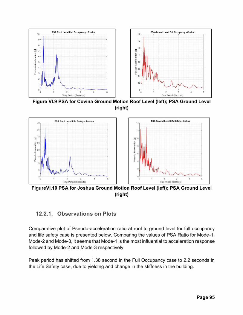
Page 95
Figure VI.9 PSA for Covina Ground Motion Roof Level (left); PSA Ground Level
(right)
FigureVI.10 PSA for Joshua Ground Motion Roof Level (left); PSA Ground Level
(right)
12.2.1. Observations on Plots
Comparative plot of Pseudo-acceleration ratio at roof to ground level for full occupancy
and life safety case is presented below. Comparing the values of PSA Ratio for Mode-1,
Mode-2 and Mode-3, it seems that Mode-1 is the most influential to acceleration response
followed by Mode-2 and Mode-3 respectively.
Peak period has shifted from 1.38 second in the Full Occupancy case to 2.2 seconds in
the Life Safety case, due to yielding and change in the stiffness in the building.

Page 96
Figure VI.11 Comparison of PSA Ratio between Full Occupancy and Life Safety
Case
From Figure VI.11, it is evident that for life safety type ground motion (more intensive)
shift in time period for all three modes has occurred. Hence, when the structure enters
non-linear range, it is governed by predominant or effective period which depends on
the intensity of the ground motion.

Page 97
12.3. Core Wall
The envelope of the maximum and minimum axial forces in the core walls is shown in
Figure VI.12 for the Life Safety case ( 2x YERMO, 2x JOSHUA, 2x CASTAICO).
Figure VI.12 Maximum and Minimum Axial Forces in the Core Walls, Life Safety
Case
The envelope of the maximum bending moments in EW and NS directions are shown in
Figures VI.13 and VI.14 respectively.

Page 98
Figure VI.13 Maximum and Minimum Bending Moment in Core Walls EW, Life
Safety Case
Figure VI.14 Maximum and Minimum Bending Moment in Core Walls NS, Life
Safety Case

Page 99
The influence of coupling beams could be seen on the bending moment in the EW
direction, “Christmas Tree” effect.
The envelope of the shear forces in NS and EW directions, together with shear force
obtained using the ACI 318-14 and ASCE 7-16 prescriptive design requirements, are
shown in Figures VI.15 and VI.16.
Figure VI.15 Maximum and Minimum Shear in Core Walls EW, Life Safety Case
with ASCE 7-16 Prescriptive Design

Page 100
Figure VI.16 Maximum and Minimum Shear in Core Walls NS, Life Safety Case
with ASCE 7-16 Prescriptive Design
Big deviation could be noticed between the shear force obtained using ACI 318-14 and
ASCE 7-16 prescriptive design and the values obtained using performance based design
(more than 300%). Buildings designed using prescriptive design procedures will meet the
standard but will not prevent a shear failure in the case of MCE.
The core wall has been redesigned for shear for floors 1-5, and for floors 6-14 as shown
in the Table VI.1 and Table VI.2 respectively.

Page 101
Table VI.1 Shear Reinforcement Redesign (Floor 1-5)

Page 102
Table VI.2 Shear Reinforcement Redesign (Floors 6 - 14)

Page 103
12.4. Design Detail Comparison
Core Wall Design Linear Model Non-linear Model
Core Wall Design
Longitudinal
#11 bars at 7 in. OC (Floors 1 - 5)
#8 bars at 7 in. OC (Floors 6 - 14)
#11 bars at 7 in. OC (Floors 1 - 7)
#8 bars at 7 in. OC (Floors 8 - 14)
Transverse (E-W)
#4 bars at 5 in. OC (Floors 1 - 5)
#4 bars at 6 in. OC (Floors 6 - 14)
#5 bars at 2 in. OC (Floors 1 - 5)
#5 bars at 5 in. OC (Floors 6 - 14)
Transverse (N-S)
Same as E-W
2 bundled #5 bars at 3 in. OC (Floors 1 - 5)
#5 bars at 3 in. OC (Floors 6 - 14)
Boundary Elements
Longitudinal #11 bars at 6 in. OC #11 bars at 6 in. OC
Transverse
24 in. long Longitudinal: #11 bars at 6
in. OC Transverse: #4 bars at 3
in. OC
24 in. long Longitudinal: #11 bars at 6 in. OC
Transverse: #5 bars at 2 in. OC
f’c Floors 1-2 6000 psi 10000 psi
Table VI.3 Design Detail Comparison of Linear and Nonlinear Model
12.5. Detailed Drawing
Detailed Drawing is attached in Appendix A.

Page 104
12.6. Diaphragm
Using the latest nonlinear model (Model V with 3 pairs of ground motions for Life Safety
and 3 pairs of ground motions for Full Occupancy), the maximum of the peak NS and the
maximum of the peak EW roof total accelerations (in g) for the three MCER ground
motions have been obtained. Stringer-panel analysis for the entire roof diaphragm in the
NS and EW directions was performed. The stringer and panel demands calculated from
the NS and EW total roof accelerations were overlaid and the design envelopes were
computed.
The panels and stringers (chords and collectors) connecting the diaphragm and the core
wall were designed for the largest NS and EW acceleration.
Table VI.4 shows the maximum and minimum roof acceleration in EW and NS directions
(maximum of 4 corner joints of the core walls), for the three pairs of Life Safety ground
motions ( 2x YERMO, 2x JOSHUA, 2x CASTAICO), in in/sec^2 and in g consequently.
EW (Ux) [in / sec ^2] NS (Uy) [in / sec ^2]
Max 520.4 511.9
Min -502.9 -508.2
EW (Ux) [g] NS (Uy) [g]
Max 1.35 1.33
Min -1.30 -1.32
Table VI.4 maximum and minimum roof acceleration for Life Safety
Table VI.5 shows the maximum and minimum roof acceleration in EW and NS directions
(maximum of 4 corner joints of the core walls), for the three pairs of Full Occupancy
ground motions ( 2x POMONA, 2x COVINA, 2x PASADENA), in in/sec^2 and in g
consequently.

Page 105
EW (Ux) [in / sec ^2] NS (Uy) [in / sec ^2]
Max 120.4 131.4
Min -502.9 -508.2
EW (Ux) [g] NS (Uy) [g]
Max 0.31 0.34
Min -0.26 -0.33
Table VI. 5 maximum and minimum roof acceleration for Full Occupancy
From both tables above, the maximum roof acceleration in EW direction is 520.4 in/sec^2
(1.35 g), in NS direction is 511.9 in/sec^2 (1.33 g).
The floor mass could be calculated by:
- RC plate mass:
area * thickness * unit weight of RC = 90*90 * 8/12 * 150 /1000 = 810 kips
- Superimposed mass:
Area * sum of superimposed dead load 90*90 * 40/1000 = 324 kips
------------------
Sum =1134 kips
ETABS gives 14th floor mass as 3.424 kip-s2/in, by multiplying by g=386.089 in/sec2
gives 1322 kips. This is because ETABS considers the weight of walls and columns as
well.
The total earthquake force in EW direction is
𝐹 = 𝑚𝑎 = 1134𝑘𝑖𝑝𝑠 ∗ 1.35𝑔 = 1531 𝑘𝑖𝑝𝑠
The total earthquake force in NS direction is
𝐹 = 𝑚𝑎 = 1134𝑘𝑖𝑝𝑠 ∗ 1.33𝑔 = 1508 𝑘𝑖𝑝𝑠
The force is distributed on each panel according to each area as:
𝐹panel=𝐹 ∗ 𝑃𝑎𝑛𝑒𝑙 𝐴𝑟𝑒𝑎/ 𝑇𝑜𝑡𝑎𝑙 𝐴𝑟𝑒𝑎
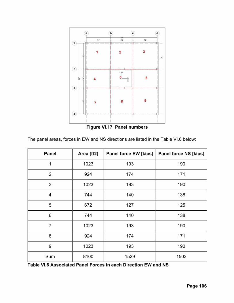
Page 106
Figure VI.17 Panel numbers
The panel areas, forces in EW and NS directions are listed in the Table VI.6 below:
Panel Area [ft2] Panel force EW [kips] Panel force NS [kips]
1 1023 193 190
2 924 174 171
3 1023 193 190
4 744 140 138
5 672 127 125
6 744 140 138
7 1023 193 190
8 924 174 171
9 1023 193 190
Sum 8100 1529 1503
Table VI.6 Associated Panel Forces in each Direction EW and NS

Page 107
The following figures shows the calculations of the Panel and Stringers in EW (and WE)
direction:
Figure VI.18 Panel Forces, EW
Figure VI.19 Forces Applied on Corners of the Panels (Panel forces divided by
four), EW

Page 108
Figure VI.20 Forces Applied on Corners of the Panels, Shear Flow Along the
Edges, EW
Figure VI.21 Axial Force Diagram for Stringers 1 & 4, EW

Page 109
Figure VI.22 Axial Force Diagram for Stringers 2 & 3, EW
Figure VI.23 Axial Force Diagram for Stringers A & D, EW

Page 110
Figure VI.24 Axial Force Diagram for Stringers C & B, EW
The following figures shows the calculations of the Panel and Stringers in NS direction:
Figure VI.25 Panel Forces, NS

Page 111
Figure VI.26 Forces Applied on Corners of the Panels (Panel forces divided by
four), NS
Figure VI.27 Forces Applied on Corners of the Panels, Shear Flow Along the
Edges, NS

Page 112
Figure VI.28 Axial Force Diagram for Stringers 1 & 4, NS
Figure VI.29 Axial Force Diagram for Stringers 2 & 3, NS

Page 113
Figure VI.30 Axial Force Diagram for Stringers A & D, NS

Page 114
Figure VI.31 Axial Force Diagram for Stringers C & B, NS
Panel Design:
Maximum shear flow from the figures above is 4.52 kip/ft.
No additional shear reinforcement is needed in the slab.

Page 115
Stringer Design:
Maximum tensile force from the figures above is 223.5 kips, the required reinforcement is
calculated as follows:
Stringer Reinforcement at peak load, and at a distance of 8’ from edge
For constructional reasons, the width of the stringer is chosen so that the reinforcement
ratio is less than 2% (preferable 1.5%). Detailing is shown in Figure VI.32 for the stringer
in the middle of the slab and at a distance of 8’ from slab edge.

Page 116
Figure VI.32 Stringer Detailing at the Center of the Building (top), and at 8’
Distance from the Slab Edge (bottom)

Page 117
12.7. Fire Sprinkler System
The sprinkler system shall remain functional at Life Safety. A fire sprinkler piping system
has been designed and will be placed hanging from the roof. The performance objective
for the piping system has been checked for both Fully Operational and Life Safety levels,
and in the context of this project, only for the building response in the NS direction.
The fundamental period of this system and effective viscous damping ratio have been
determined from a field test. Displacement record for freely vibrating sprinkler is shown in
Figure VI.33
Figure VI.33 Displacement Record for Freely Vibrating Sprinkler in NS Direction
From this figure the period could be calculated from average time between four
consequent peaks. Damping could be calculated from equation:
𝜁 =
𝜋𝑗𝑙𝑛
𝑢𝑖
𝑢𝑖+𝑗 (Chopra, Equation 2.2.14)
Where:
𝜁 is the damping ratio
𝑢𝑖 is the displacement at peak number 𝑖
𝑢𝑖+𝑗 is the displacement at peak number 𝑖 + 𝑗

Page 118
Peak 1 Peak 5
Time [sec.] 0.096 1.716
Amplitude 0.1275 0.0308
Delta-T [sec.] Nr. of peaks Period [sec.] amping
1.620 4 0.405 5.65%
Note that the calculated damping ratio depends on the range of the movement, in case
of 8 peaks, the damping would be 5.21% instead of 5.65% with 4 peaks.
Peak 1 Peak 9
Time [sec.] 0.096 3.060
Amplitude 0.1275 0.0093
Delta-T [sec.] Nr. of peaks Period [sec.] Damping
2.964 8 0.371 5.21%
A preliminary analysis shows that the threaded connections can satisfactorily, that is
without leaking, resist 18 mm relative floor-pipe displacement demands. With the
calculated period of 0.405 second and effective viscous damping ratio of 5.65 %, the
displacement response and the usage ratio of the piping system has been defined as
follows:
Full Occupancy motion (e.g. Covina)
Max. Displacement = 8.88 mm Usage Ratio = 8.88/18 = 49 % OK Life Safety motion (e.g. Joshua) Max. Displacement = 61.34 mm Usage Ratio = 61.34 /18 = 341 % N.G. The excessive displacement could be mitigated by adding additional seismic bracing on the piping to limit the movement of the pipe.

Page 119
12.8. Overhanging Projector
Considering a projector hanging of the slab level 14 of the building (roof). A free vibration
test for displacement was carried out for the projector, only NS direction will be
considered, Figure VI.34. The fundamental period (Tn, sec) and the percentage of critical
damping from the test data (ξ) has been calculated as below:
𝜁 =
𝜋𝑗𝑙𝑛
�̈�𝑖
�̈�𝑖+𝑗 (Chopra 5th edition, Equation 2.2.14)
Where:
𝜁 is the damping ratio
�̈�𝑖 is the acceleration at peak number 𝑖
�̈�𝑖+𝑗 is the acceleration at peak number 𝑖 + 𝑗
Figure VI.34 Acceleration Record for Freely Vibrating Projector in NS Direction

Page 120
Peak 1 Peak 5
Time [sec.] 0.160 0.772
Amplitude 0.337 0.195
Delta-T [sec.] Nr. of peaks Period [sec.] Damping
0.612 4 0.153 2.18%
Peak 1 Peak 11
Time [sec.] 0.160 1.672
Amplitude 0.337 0.099
Delta-T [sec.] Nr. of peaks Period [sec.] Damping
1.512 10 0.151 1.95%
The calculated damping ratio depends on the range of the movement considered too, in
case of 4 peaks the damping is 2.18%, in case of 10 peaks it is 1.95%.
Using the spectra, the maximum seismic force in the projector corresponding to its period
Tn=0.15 sec and weight (36 lb) has been calculated. With this force and the weight,
factorized tensile and shear forces in the anchorage system could be determined. This is
shown in the table and figure below.

Page 121
Using anchors KWIK Bolt TZ carbon steel, Hilti Volume 2: Anchor Fastening Technical
Guide, Edition 1.

Page 122
PART VII: Conclusion
An idea of performance based seismic design, that stems from analyzing nonlinear
response of the structure, is well justified given the merits in terms of better predictability
of structure performance compared to linear model. In conclusion, few learnings worth
taking note of are discussed below:
● Nonlinear, performance based seismic design, although time consuming and
expensive process, was the correct choice for the structure analysis. Had only
linear design been used, the transverse reinforcement would not have been
enough to withstand an MCE level earthquake, and a plastic hinge would have
formed at floor 6 instead of at the bottom of the building as intended.
● Nonlinear behavior is far more accurate at predicting the response of concrete, as
it is a nonlinear material when used for seismic design.
● Nonlinear response is governed by the predominant period which is intensity
dependent and hence, one can not uniquely predict modal properties of the
structure while considering nonlinear response of the structure.
● The structure subjected to nonlinear response, with effective coupling beam
model, can better predict the distribution of shear between coupled lateral force
resisting system. Hence, the design of lateral force resisting system for shear
demand can be done for higher shear demand.
● Resilience Base Seismic Design (RBSD) also proved why nonstructural
components need to be properly detailed for earthquakes if they are to be
operational after an earthquake. Even if the building structure manages to
withstand the earthquake, the building cannot be operational with broken
sprinklers, generators, utilities, etc.
● The cost of damage after an earthquake could be so high that the building may
need to be demolished. This reasoning can help engineers explain to owners the
economic benefits of PBSD and RBSD.
● Despite of all advanced computational framework, human error must be
considered. Everyone in this project got different results, although everyone
started with the same basic model. This uncertainty, which looks random at this
moment, it will be gradually reduced with better human machine interface that will
be able to post-process the data more efficiently. The review process for PBSD
needs to be extensive if it is to be used correctly. Hopefully one day PBSD will
become more common in practice, and the human error could be decreased as it
becomes more developed.

b
b
c
c
d
d
1 1
2 2
3 3
4 4
b1 c1
28' - 0"
a
a
31' - 0" 31' - 0"
33
' - 0
"
24
' - 0
"
33
' - 0
"10' - 6"
Scale
Project number
Date
Drawn by
Checked by
www.k1michel.com
1" = 20'-0"
4/2
4/20
20
2:3
4:1
5 A
M
S.001
Plan View, Level 2Project Number
Mr. Richman
14 Story Bldg in LAIssue Date
Author
Checker
No. Description Date
1" = 20'-0"1 Level 2

TY
P 4
.9"
#4 @4" - 14
#4 @2" - 26
#4 @2" - 15
#10 - 32
#4 @5" - 43
#4 @5" - 22
#3 @5" - 27
2' -
6"
-
---S.002
Level 00' - 0"
Level 116' - 0"
2
4' -
9"
16
' - 0
"
0' -
8"
5' -
0"
Scale
Project number
Date
Drawn by
Checked by
www.k1michel.com
As indicated
4/2
4/20
20
2:3
4:1
5 A
M
S.002
Boundary ElementProject Number
Mr. Richman
14 Story Bldg in LAIssue Date
Author
Checker
No. Description Date
1/4" = 1'-0"2 Section 2

2 2
3 3
b1
b1
c1
c1
Boundary Element
#10 @6 3/16" - 32
#4 @5" - 43
#4 @5" - 22
#3 @5" - 27
#4 @5" - 6#4 @5" - 6
#3 @5" - 29
11' - 9"
26
' - 6
"
Scale
Project number
Date
Drawn by
Checked by
www.k1michel.com
1/4" = 1'-0"
4/2
4/20
20
2:3
4:1
5 A
M
S.003
Walls ReinforcementProject Number
Mr. Richman
14 Story Bldg in LAIssue Date
Author
Checker
No. Description Date1 Revision 1 Date 1
1/4" = 1'-0"1 Level 2 _Walls

Level 228' - 0"
3
2 #6 @ 5"
#4 @ 5" -42
#4 @ 5" -41
#11 @ 5" -37
Level 00' - 0"
Level 116' - 0"
Level 228' - 0"
b cc1
1
S.004
S.004
Scale
Project number
Date
Drawn by
Checked by
www.k1michel.com
As indicated
4/2
4/20
20
2:3
4:1
8 A
M
S.004
Coupling BeamsProject Number
Mr. Richman
14 Story Bldg in LAIssue Date
Author
Checker
No. Description Date
1/4" = 1'-0"1 Section 4
1/8" = 1'-0"3 South


![SEISMIC PERFORMANCE AND ECONOMIC …SEISMIC PERFORMANCE AND ECONOMIC FEASIBILITY ... ... 4]](https://img.pdfslide.us/doc/110x75/5e730ef63a752763c8260684/seismic-performance-and-economic-seismic-performance-and-economic-feasibility-.jpg)