TECHNICAL REPORT ____________________________________________________________________________________________________________________

Title: Wind field simulations at Askervein hill

____________________________________________________________________________________________________________________

Client: Internal study

____________________________________________________________________________________________________________________

Date: October 1999 Number of pages: 37

____________________________________________________________________________________________________________________

Contract: - Classification: -

____________________________________________________________________________________________________________________

Author(s): Jerome Leroy, Stage ingeneur, Ecole Centrale de Nantes

___________________________________________________________________________________________________________________

Responsible: Arne Reidar Gravdahl, VECTOR AS

____________________________________________________________________________________________________________________

Distribution: -

Archive: VECTOR_9910_100

VE C T O R

C F D C O N S U L T I N G

VECTOR AS Phone: +47 33 38 18 00 E-mail: vector@vector.no Industrigaten 9 Telefax: +47 33 38 18 08 Internet: vector.no N-3117 Tønsberg Enterprise no.: NO 967 070 513 Norway

- 2 -

Abstract : This report presents the study that has been carried out from August to October 1999 in the VECTOR company by Jérôme LEROY, student at the Ecole Centrale de Nantes. VECTOR has been developing a wind code called WindSim these last years. The Askervein hill case, one of the most complete experimental study concerning full scale wind data measurements, is used in this study to test WindSim. The study of this particular case could be helpful towards the goal of meso scale atmospheric boundary layer modelling.

Acknowledgements : I want to thank Arne Reidar Gravdahl, who supervised this work, for his great welcome and his alertness. I also want to thank the rest of the Vector crew for their help and fellow feeling during my staying in Norway.

- 3 -

1. INTRODUCTION............................................................................................................. 4

1.1. THE HOST COMPANY......................................................................................................... 4 1.2. THE WINDSIM PROJECT.................................................................................................... 4

1.2.1. Electricity in Norway ................................................................................................ 4 1.2.2. Wind resources in Norway ........................................................................................ 5 1.2.3. Description of the project.......................................................................................... 5

1.3. SUBJECT OF THE PRESENT STUDY...................................................................................... 6 1.4. THE ASKERVEIN HILL CASE : BACKGROUND INFORMATION.............................................. 6

2. DESCRIPTION OF THE STUDY................................................................................... 8

2.1. PRELIMINARY ASSUMPTIONS............................................................................................. 8 2.2. TURBULENCE MODEL........................................................................................................ 8

2.2.1. Mixing length model.................................................................................................. 8 2.2.2. k-ε model ................................................................................................................... 9 2.2.3. Two scale k-ε model ................................................................................................ 10

2.3. NUMERICAL SETUP.......................................................................................................... 11 2.3.1. Calculation domain ................................................................................................. 11 2.3.2. Boundary conditions ............................................................................................... 11

3. SIMULATIONS AND RESULTS .................................................................................... 15

3.1. GRID TESTING................................................................................................................. 15 3.1.1. Number of cells........................................................................................................ 15 3.1.2. Grid grading............................................................................................................ 21

3.2. INLET PROFILES............................................................................................................... 26 3.3. BOUNDARY CONDITIONS................................................................................................. 26 3.4. TURBULENCE MODEL...................................................................................................... 29

4. CONCLUDING REMARKS ............................................................................................ 34

5. REFERENCES................................................................................................................... 36

- 4 -

1. INTRODUCTION

1.1. The host company I have done my internship in a Norwegian company called Vector. Vector is a CFD consulting company. It is located in Tønsberg, a town that lays on the western part of the Oslofjord, 100 km south of the capital of Norway. This business was created in 1993 by Arne Reidar GRAVDAHL, who supervised this work. Vector has realised several studies for Statoil, the major oil company in Norway. Currently is developing Vector a wind code in collaboration with the Norwegian Water Resources and Energy Administration.

1.2. The WindSim project

1.2.1. Electricity in Norway For the last decades, Norway has relied exclusively on hydroelectricity. But the electricity provided by water resources has turned out to be insufficient during the last years. Norway is no more independent from the energy point of view and has had to import electricity to supply its growing national demand. Therefore the Norwegian Water Resources and Energy Administration (NVE) decided to get interested in other renewable sources of energy. Wind energy proved to be an interesting option, considering the Norwegian wind resources.

Figure 1.1.Estimate of wind resources in Scandinavia

(mean wind speed in open terrain 50 meters above the ground)

- 5 -

1.2.2. Wind resources in Norway Norway is a country with rich wind resources. Still, their exploitation has been very modest so far. A cost effective energy production is only obtainable after careful positioning of wind turbines. The energy content of a wind field is proportional to the cube of the wind speed. Obviously, the energy production is most sensitive to varying wind conditions. The ideal situation would be to have historical data on wind speed and direction for every potential locations for wind turbines. This information is of course not available, but a combination of experimental and numerical methods can help to achieve this goal. Thus, the recent interest in wind energy has driven the NVE to launch a project on meso scale wind modelling.

1.2.3. Description of the project The project currently undertaken aims at assessing the wind resources along the Norwegian coast. Local models are established from the southern tip of Norway to the Russian border in the north. The wind resources are estimated on a so called meso scale. Available information on wind resources depends on which length scale phenomenon is considered. One can put in evidence three length scales. The synoptic scale typically covers whole countries. An estimate of the wind resources in Norway, Sweden and Finland has been established by the U.S. National Renewable Energy Laboratory (see figure 1.1). It shows the mean wind speed in open terrain 50 meters above the ground. The hatched area indicates hilly terrain. The figure, as can be seen, puts into evidence interesting wind resources along the Norwegian coast. The meso scale covers regions in the order of 100 km2. In contrast to the synoptic scale, on the meso scale the influence of local topography is included. It is well known that topographically induced speedups can be substantial. One must take advantage of these speedups when locating wind farms.

Figure 1.2. Meso scale models along the Norwegian coast

on which windfields are calculated

- 6 -

The micro scale covers typically an area in the order of 1 km2. On this scale, vegetation, infrastructure and the mutual interaction between wind turbines is important. Before any wind farm construction, information on the local windfields on this scale will naturally be obtained both experimentally and numerically. WindSim is a simulator for prediction of local wind fields, based on 3-D digital terrains models. Its main goal is the assessment of wind resources along the Norwegian coast. There are also other applications. WindSim is also used in prediction of dispersion of air pollution on a local scale. Accumulated exposure from continuous sources is determined from statistical weather data. During an uncontrolled release the dispersion scenario is calculated from a local weather forecast and input about the amount, position, time etc. given by the user. Other fields are concerned, for instance civil engineering. In certain locations, the wind load on buildings is important and must be taken into account. It can be interesting to have a precise idea of the wind field to design these buildings. Aviation safety is also a matter of interest in hazardous conditions such as mountainous terrain, where inhomogeneous flow can be observed : the airplane crash at Værøy Island in 1990 is an example (T. UTNES and K.J. EIDSVIK, 1996).

1.3. Subject of the present study The present study aims at testing WindSim on a known case (topography and experimental results) according to different parameters in order to improve the results. The conclusions of the study will help towards the goal of micro scale modelling. In order to test the results yielded by WindSim, they are compared with experimental data. The major experimental study that has been undertaken in this field is certainly the Askervein hill project. This project is regarded as a reference when it comes to test simulation of flow over hills, both in experimental and numerical studies.

1.4. The Askervein Hill case : background information This project was a collaborative study carried out under the auspices of the International Energy Agency Programme of R&D on Wind Energy Conversion System. The experiments were conducted in 1982 and 1983 on Askervein, a 116 meters high hill on the west coast of the island of South Uist in the Outer Hebrides of Scotland. The site was selected considering many goals such as suitability from a numerical point of view, easy access, good wind conditions (uniform and well defined direction), topography. The hill is nearly ellipsoidal in plan with minor and major axis of 1 and 2 kilometres respectively. It is the site of the most complete field experiment to date, with 50 towers deployed, and whose 27 of them were equipped with three component turbulence sensors.

- 7 -

A

AA HT

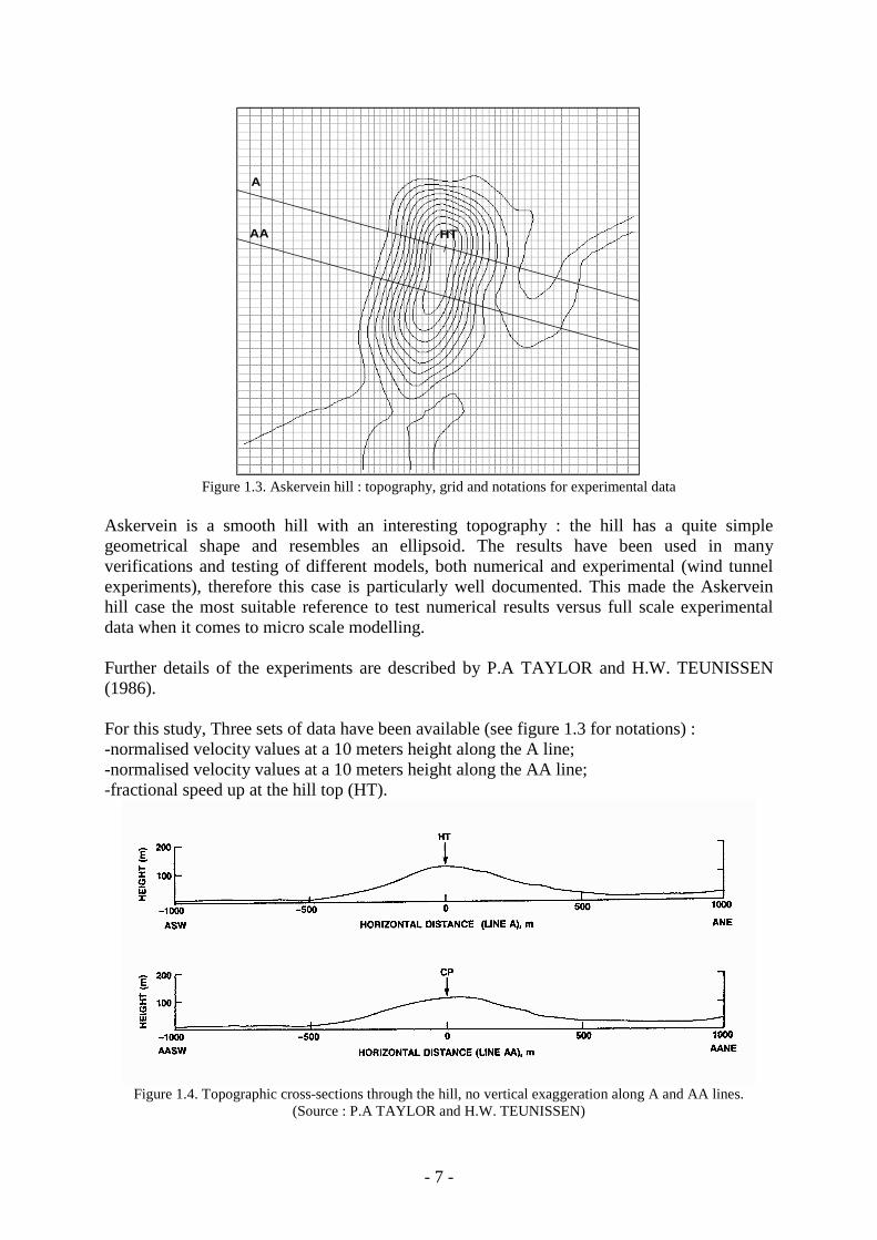
Figure 1.3. Askervein hill : topography, grid and notations for experimental data

Askervein is a smooth hill with an interesting topography : the hill has a quite simple geometrical shape and resembles an ellipsoid. The results have been used in many verifications and testing of different models, both numerical and experimental (wind tunnel experiments), therefore this case is particularly well documented. This made the Askervein hill case the most suitable reference to test numerical results versus full scale experimental data when it comes to micro scale modelling. Further details of the experiments are described by P.A TAYLOR and H.W. TEUNISSEN (1986). For this study, Three sets of data have been available (see figure 1.3 for notations) : -normalised velocity values at a 10 meters height along the A line; -normalised velocity values at a 10 meters height along the AA line; -fractional speed up at the hill top (HT).

Figure 1.4. Topographic cross-sections through the hill, no vertical exaggeration along A and AA lines.

(Source : P.A TAYLOR and H.W. TEUNISSEN)

- 8 -

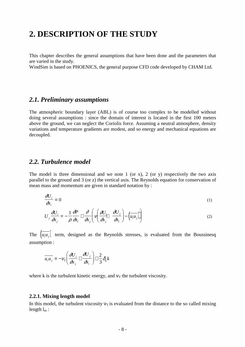
2. DESCRIPTION OF THE STUDY This chapter describes the general assumptions that have been done and the parameters that are varied in the study. WindSim is based on PHOENICS, the general purpose CFD code developed by CHAM Ltd.

2.1. Preliminary assumptions The atmospheric boundary layer (ABL) is of course too complex to be modelled without doing several assumptions : since the domain of interest is located in the first 100 meters above the ground, we can neglect the Coriolis force. Assuming a neutral atmosphere, density variations and temperature gradients are modest, and so energy and mechanical equations are decoupled.

2.2. Turbulence model The model is three dimensional and we note 1 (or x), 2 (or y) respectively the two axis parallel to the ground and 3 (or z) the vertical axis. The Reynolds equation for conservation of mean mass and momentum are given in standard notation by :

∂∂U

xi

i

= 0 (1)

( )UU

x

P

x x

U

x

U

xu uj

i

j i j

i

j

j

ii j

∂∂ ρ

∂∂

∂∂

ν∂∂

∂∂

= − + +

−

1 (2)

The ( )u ui j term, designed as the Reynolds stresses, is evaluated from the Boussinesq

assumption :

u uU

x

U

xki j T

i

j

j

iij= − +

+ν

∂∂

∂∂ δ

2

3

where k is the turbulent kinetic energy, and νT the turbulent viscosity.

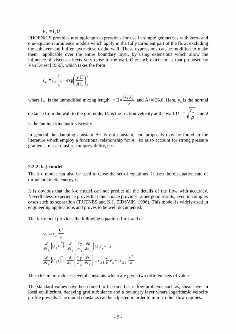
2.2.1. Mixing length model In this model, the turbulent viscosity νT is evaluated from the distance to the so called mixing length lm :

- 9 -

UlmT =ν

PHOENICS provides mixing-length expressions for use in simple geometries with zero- and one-equation turbulence models which apply in the fully turbulent part of the flow, excluding the sublayer and buffer layer close to the wall. These expressions can be modified to make them applicable over the entire boundary layer, by using extensions which allow the influence of viscous effects very close to the wall. One such extension is that proposed by Van Driest [1956], which takes the form:

++−=

A

yll mm exp10

where lm0 is the unmodified mixing length, ντ gyU

y =+ and A+= 26.0. Here, yg is the normal

distance from the wall to the grid node, Uτ is the friction velocity at the wall ρ

ττ

wU = and ν

is the laminar kinematic viscosity. In general the damping constant A+ is not constant, and proposals may be found in the literature which employ a functional relationship for A+ so as to account for strong pressure gradients, mass transfer, compressibility, etc.

2.2.2. k-εεεε model The k-ε model can also be used to close the set of equations. It uses the dissipation rate of turbulent kinetic energy ε. It is obvious that the k-ε model can not predict all the details of the flow with accuracy. Nevertheless, experience proves that this choice provides rather good results, even in complex cases such as separation (T.UTNES and K.J. EIDSVIK, 1996). This model is widely used in engineering applications and proves to be well documented. The k-ε model provides the following equations for k and ε :

ν εµT ck

=2

( )

( )

∂∂

∂∂

ν

σ∂∂ ε

∂∂ ε

∂∂

ν

σ ε

∂ ε∂ ε

εε

ε

xi

Ui

kx

i

T

k

k

xi

Pk

xi

Ui x

i

Tx

ic

kP

kc

k

=

+ −

=

+ −

1 2

2

This closure introduces several constants which are given two different sets of values. The standard values have been tuned to fit some basic flow problems such as, shear layer in local equilibrium, decaying grid turbulence and a boundary layer where logarithmic velocity profile prevails. The model constants can be adjusted in order to mimic other flow regimes.

- 10 -

Considering a neutral ABL, the standard k-ε model is unable to reproduce the right level of turbulence in the weak shear layer away from the ground. In this region the turbulent viscosity is overpredicted, (DETERING and ETLING, 1985). The standard model constants have been modified in an attempt to improve the situation. The value of Cε2, determined from experiments with decaying grid turbulence, remains unchanged. The diffusion constant σk, close to unity following Reynolds analogy, also remains unchanged. However, the constant Cµ, determined from a shear layer in local equilibrium where it is found to be equal to :

u u1 22

κ

, has been reduced in accordance with measurements in the ABL (Panofsky, 1977).

Finally, the constants Cε1 and Cε2 can be adjusted, guided by the relation from a boundary layer where the logarithmic law is valid :

C Cε εµ ε

κσ1 2

2

= −C

Note that κ is the Von Karman constant, set to be 0.4. The different values of the model constants tested in this work are given in the table below

Constants names Cµ Cε1 Cε2 σk σε Standard values 0.09 1.44 1.92 1.0 1.3 Modified values 0.0324 1.44 1.92 1.0 1.85

2.2.3. Two scale k-εεεε model In this model the total turbulence energy, k, is divided equally between the production range and transfer range, thus k is given by :

tp kkk +=

where kp is the turbulent kinetic energy of eddies in the production range and kt is the energy of eddies in the dissipation range. For high turbulent Reynolds numbers, the transport equations for the turbulent kinetic energies are:

( )( ) ( )pk

i

p

p

T

ip

i

pp

x

k

kCx

Uk

xt

kερρνρ

ρ−=

∂∂

−∂∂

∂∂+

∂∂

( ) ( ) ( )tpi

t

t

Tt

iit x

k

kCk

x

U

xk

tεερρνρρ −=

∂∂

−∂∂

∂∂+

∂∂

wherein; εp is the transfer rate of turbulent kinetic energy from the production range to the dissipation range; εt is the dissipation rate; pk is the volumetric production rate of turbulent kinetic energy; and C(kp) and C(kt) are constant coefficients. The corresponding transport equations for the energy transfer rate and the dissipation rate are given by :

- 11 -

( )( ) ( )2

322

1 pppkpkppi

p

p

T

ip

i

pCpCpC

kxCx

U

xtεερε

ερνρε

ρε−+=

∂∂

−∂∂

∂∂+

∂∂

( )( ) t

ttpttpt

i

t

t

T

it

i

t

k

CCC

xCx

U

xt

232

21 εεεε

ρεε

ρνρερε −+=

∂∂

−∂∂

∂∂+

∂∂

where C(εp), C(εt), Cp1, Cp2, Cp3, Ct1, Ct2 and Ct3 are constant model coefficients. The Cp1pk

2/kp and Ct1ε2/kt terms can be interpreted as variable energy transfer functions. The former term increases the energy transfer rate when production is high, and the second term increases the dissipation rate when the energy transfer rate is high. The model constants are given as:

C(kp) C(εp) C(kt) C(εp) Cp1 Ct2 Ct3 C1 Ct2 Ct3 0.75 1.15 0.75 1.15 0.21 1.24 1.84 0.29 1.28 1.66

The eddy viscosity is computed from:

tT

kC

εν µ

2

=

The model may be used in combination with equilibrium (GRND2) or non-equilibrium (GRND3) wall functions (see part 2.3.2.2).

2.3. Numerical setup

2.3.1. Calculation domain The physical domain is discretised with a 54*44 grid covering an area of about 3000 meters in x and y directions. The height of the domain is fixed at 1100 meters, with a variable number of cells and a variable geometrical distribution, who are tested in this study.

2.3.2. Boundary conditions 2.3.2.1. Inflow Two different inlet profiles have been tested. First, inlet profiles for velocity, kinetic energy and dissipation rate of kinetic energy are given by the following analytical expressions :

UU z

z10

=

* l nτ

κ for z<500m

U m s111 0= −. for z≥500m

kU

C

z

L B L

= −

*

2 2

1µ

- 12 -

ε κ= +

U

z L o b u k o v

*3 1 4

Where U* is calculated so that there is no discontinuity in the velocity profile at z=500m, LBL is the thickness of the boundary layer, and Lobukov is a parameter set to be equal to 1000 m. Another inlet profile is also tested in this study. This profile is fully developed, meaning that it is obtained by running the simulator on a flat computational domain. In practice, this profile is obtained by letting the model run itself on a 3 cells long computational domain having the same number of cells and distribution in y and z directions than the Askervein hill domain. The inlet condition is cyclic, that is to say that the outflow is constantly applied at the inlet of the domain. This is equivalent to compute the flow resulting from a constant profile on a long flat uniform terrain. Pressure is calculated at each node on the boundary, according to velocity so that the equation of continuity is satisfied (“mass flow” boundary condition). 2.3.2.2. Ground boundary On the ground, the law of the wall is applied, in order to bridge the viscous sublayer and cut computational costs. Thus, we apply "near-wall" boundary conditions for the mean flow and turbulence transport equations. It gives the value of the dependant variables at the first cell row above the ground. These grid nodes are presumed to lie outside the viscous sublayer in a fully turbulent flow. This approach reduces computation time and moreover simplifies computation outside the layer since viscous effects do not need to be taken into account any more. PHOENICS provides 2 different types of wall functions : equilibrium log-law functions and non-equilibrium log-law functions called respectively GRND2 and GNRD3 in the PHOENICS parlance. Equilibrium log-law wall functions

U

U

E.yr

τ κ=

+

ln (1)

kU

C= τ

µ

2

2 (2)

εκ

µ=C .k

.y

. .0 75 1 5 (3)

where : ρ is the fluid density, E the roughness parameter, κ the Von Karman constant, y the distance of the first grid point to the wall, Ur the resultant velocity parallel to the wall at the first grid node, y+ the dimensionless distance to the wall given by (4):

- 13 -

yU y+ = τ

υ (4)

and Uτ the resultant friction velocity defined by (5) :

U wτ

τρ

= (5)

The law (1), the so called logarithmic law of the wall, must be applied strictly at points where 30<y+<130. The law (2) assumes that turbulence is in local equilibrium (production = dissipation). These laws are implemented in the model by way of source terms. The E factor takes the roughness into account. This parameter is considered as a function of the roughness Reynolds number :

Reττ

ν=

U Hr , where Hr is the absolute value of the equivalent sand-grain roughness height.

Hr is given a value of 0.01 m, which is the typical value for the grass and few trees vegetation of the hill.

Rer<3.7 E=Em

3.7<Rer<100 E

ab

a

Er

m

=

+

−

1

12

2

Re

Rer>100 E=b/Rer Where :

Em = 0.9

a 1 2x 3x

b 29.7

x 0.02248100 Re

Re

3 2

r

r0.564

= + −=

=−

For the 2-scale k-ε model, the following boundary conditions are applied for the turbulence variables:

βκ+

=1pk

βκβ+

=1tk

y

KCp κ

ε µ5.175.0

=

- 14 -

pt εε =

Here

2

=

µ

τ

C

UK , Y is the normal distance of the first grid point from the wall, and β is given

by:

( ) ( ) 1C-C-C p2p1p3

2

2

−=

µεβ

CC

K

p

which yields a value of β=0.25. Non equilibrium log-law wall functions

This law uses the root of the kinetic energy k rather than the friction velocity as the characteristic length scale. Thus, equation (1) is replaced by :

U k

U

E k yr t

t

2

2

2

τ κ=

ln

where

κ κ µt C= 0 2 5.

E ECt = µ0 25.

The equations (2) to (5) remain unchanged. The value of k at the near wall point is calculated from its transport equation, considering that energy diffusion is set to zero to the wall. For the2-scale k-ε model, the treatment is similar to that employed for the standard k-ε model, with kp and kt determined from their respective balance equations and for simplicity it is assumed that εp=εt. 2.3.2.3. Other boundaries On the lateral sides and on the top of the domain are imposed zero normal derivatives and zero values for velocities, k and ε. At the outlet, zero gradient boundary conditions are imposed, meaning that plane geometry downwind the domain is assumed. Pressure is set to be equal to zero.

- 15 -

3. SIMULATIONS AND RESULTS

3.1. Grid testing The grid can be modified in z direction, according to the number of cells and their distribution. The cells distribution use an arithmetic sequence, providing a convenient method for smooth grid construction. Let us call hk the height of cell number k (from the ground), we have thus : h h hk k+ = +1 ∆ . n is the total number of cells in z direction, and g is the grid grading defined by:

gh

hn

= 1

Thus the height of the first cell is given by, noting H the total height of the domain:

hH

ng

g

1

11

2

=+

−

and the arithmetic reason by :

( )

∆hH

n nc

c

=− +

−

2

1 12

1

Note that tests have been done with the k-ε model and equilibrium boundary condition, with analytical profile at the inlet. Firstable, we study the effect of varying g, with a fixed number of cells. We choose a grading g=0.1.

3.1.1. Number of cells Table shows the different tested cases, figure 3.1 shows the different grid repartitions.

Grid Number of cells in

z direction Grading

A 20 0.1 B 25 0.1 C 30 0.1 D 35 0.1

- 16 -

a b c d0.0

500.0

1000.0

1500.0

heig

ht above g

round (

m)

Tested grids

varying n

Figure 3.1. Tested grids

Note that the total height of the domain is not a constant since the hill is 116m high, but this only affect the cells height in a 10% uniform rate. The results of simulations are compared against experimental data : see respectively figures 3.2, 3.3 and 3.4 for results along lines A, AA and at the HT point. Figure 3.2 displays the first velocity component along the A line. It should be noted one of the grids catches the maximum speed up. The error is about 15% at the hill top. Grids a, b, c and d give comparable results upwind the hill. Results on the lee side vary according to the grid. As expected, the results are getting better as the number of nodes in z-direction is increasing, Figure 3.3 is similar to figure 3.2 except that it is for the AA line. As in figure 3.2, the hill top speed up is under predicted. Nevertheless maximum speed up is quite good predicted. Grids a, b, c give about the same results right up to the top. Grid c predicts maximum speed up with very good accuracy. Grid d, on the contrary, gives good results for the first measurement points but largely underpredicts the hill top speed up. On the lee side, the finer he grid is, the lower velocities are predicted. Figure 3.4 displays the fractional speed up at the hill top point defined by :

)(

)()()(

zUref

zUrefzUzS

−=∆

where Uref is the upstream the hill (without obstacles). Note that for the Askervein hill case, the reference velocity profile is chosen 500 meters upwind the hill top. This is worth to notice since the results can be affected in the order of 10% whether reference is taken at the inlet of the domain or at some other point downstream. The simulations results are interpolated from the first grid node.

- 17 -

500.0 1000.0 1500.0 2000.0 2500.0

distance along A line (m)

0.0

0.5

1.0

1.5

2.0

no

rma

lize

d v

elo

city

A line

varying n

exp results

grid a

grid b

grid c

grid d

Figure 3.2

500.0 1000.0 1500.0 2000.0 2500.0

distance along AA line (m)

0.0

0.5

1.0

1.5

2.0

no

rma

lize

d v

elo

city

AA line

varying n

exp results

grid a

grid b

grid c

grid d

Figure 3.3

- 18 -

0.0 0.5 1.0 1.5

fractionnal speed up

1

10

100

he

igh

t a

bo

ve

gro

un

d (

m)

hill top

varying n

exp results

grid a

grid a

grid c

grid d

Figure 3.4

Figure 3.4 shows the inability of the grid to predict the flow within the first meters above the ground. Results of the simulations always underpredict experimental data below 20 meters. Figures 3.5 to 3.8 show the total velocity field for the different simulations with grids a, b, c and d. Velocities are displayed at the first cell row, with contours for the first component of velocity. These results can not be compared against experimental results but can help towards further understanding of the different cases.

- 19 -

PHOTON

DTM - WINDROSE, ANGLE = 270, ID=400

X

Y

UCRT

3.5

4.0

4.5

5.0

5.5

6.0

6.5

7.0

7.5

8.0

8.6

9.1

9.6

10.1

10.6

2.72E+01

Figure 3 5. Grid a

PHOTON

DTM - WINDROSE, ANGLE = 270, ID=400

X

Y

UCRT

2.8

3.4

3.9

4.5

5.0

5.6

6.1

6.7

7.3

7.8

8.4

8.9

9.5

10.1

10.6

2.72E+01

Figure 3.6. Grid b

- 20 -

PHOTON

DTM - WINDROSE, ANGLE = 270, ID=400

X

Y

UCRT

1.9

2.6

3.2

3.8

4.4

5.0

5.7

6.3

6.9

7.5

8.1

8.8

9.4

10.0

10.6

2.72E+01

Figure 3.7. Grid c

PHOTON

DTM - WINDROSE, ANGLE = 270, ID=400

X

Y

UCRT

-0.4

0.4

1.2

2.0

2.7

3.5

4.3

5.1

5.9

6.7

7.5

8.3

9.1

9.8

10.6

2.72E+01

Figure 3.8. Grid d

- 21 -

Figures 3.5 to 3.8 put on evidence a zone of low velocities downstream the hill. This zone is varying according to the different grids. Thus, grid d shows an area with reversed flow, which means that there is separation downwind the hill. However, grid d underpredicts velocity on the lee side for both of the lines. This means that separation is not as important as it is calculated. On the other hand, it should be noted that the grid can not be refined too much towards the ground, since too thin and long cells may cause numerical inaccuracy. Then the number of cells is fixed at 30 and the grading is varied.

3.1.2. Grid grading The table below shows the different tested cases :

Grid Number of cells in

z direction Grading

e 30 0.2 f 30 0.15 c 30 0.1 h 30 0.075

Figure 3.10 shows the different grid repartitions.

c e f g0.0

500.0

1000.0

1500.0

heig

ht above g

round (

m)

Tested grids

varying g

Figure 3.10

Figures 3.11 to 3.13 display data comparisons.

- 22 -

500.0 1000.0 1500.0 2000.0 2500.0

distance along A line (m)

0.0

0.5

1.0

1.5

2.0

norm

aliz

ed v

elo

city

A line

varying g

exp results

grid e

grid f

grid g

Figure 3.11

500.0 1000.0 1500.0 2000.0 2500.0

distance along AA line (m)

0.0

0.5

1.0

1.5

2.0

norm

aliz

ed v

elo

city

AA line

varying g

exp results

grid e

grid f

grid g

Figure 3.12

- 23 -

0.0 0.5 1.0 1.5

fractionnal speed up

1.00

10.00

100.00

heig

ht above g

round (

m)

hill top

varying g

exp results

grid e

grid f

grid g

Figure 3.13

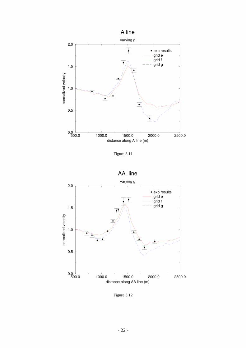
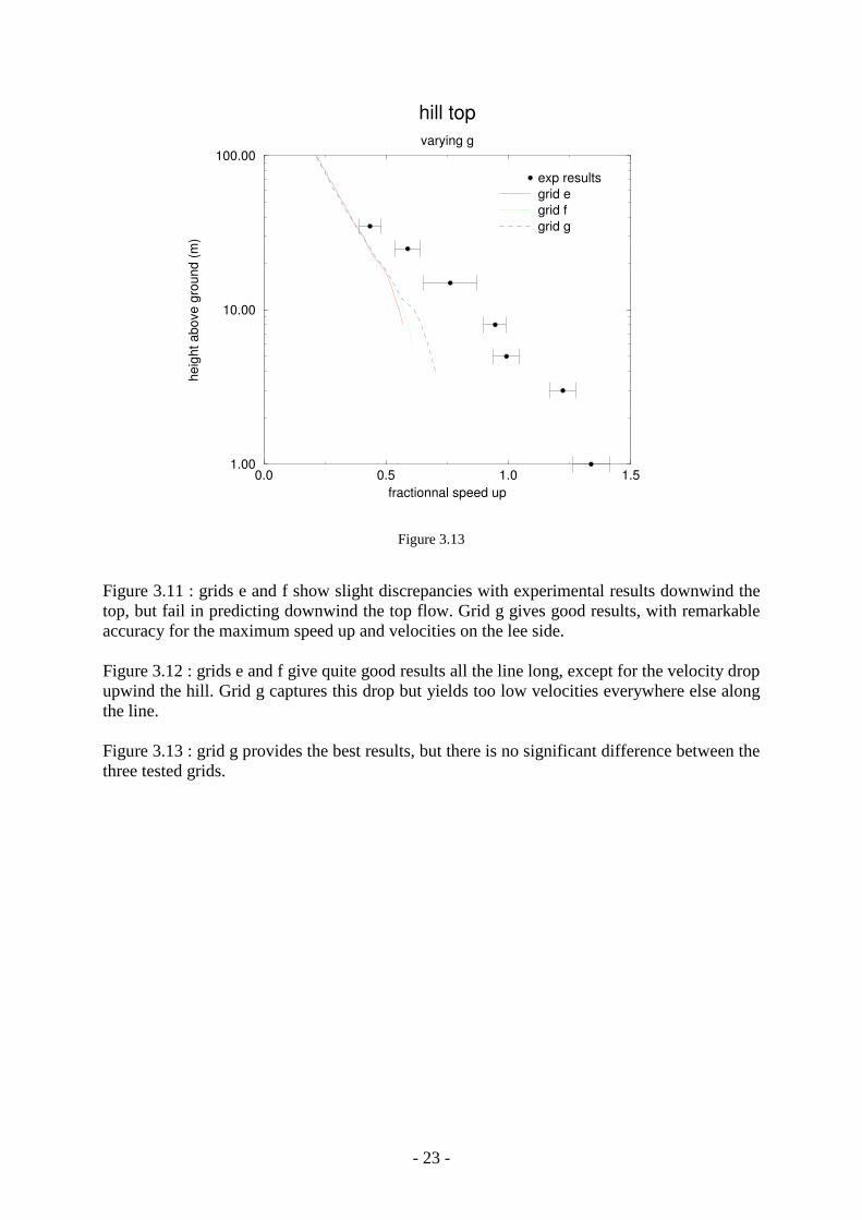
Figure 3.11 : grids e and f show slight discrepancies with experimental results downwind the top, but fail in predicting downwind the top flow. Grid g gives good results, with remarkable accuracy for the maximum speed up and velocities on the lee side. Figure 3.12 : grids e and f give quite good results all the line long, except for the velocity drop upwind the hill. Grid g captures this drop but yields too low velocities everywhere else along the line. Figure 3.13 : grid g provides the best results, but there is no significant difference between the three tested grids.

- 24 -

PHOTON

DTM - WINDROSE, ANGLE = 270, ID=400

X

Y

UCRT

3.3

3.9

4.4

4.9

5.4

6.0

6.5

7.0

7.5

8.1

8.6

9.1

9.6

10.1

10.7

2.76E+01

Figure 3.14. Grid e

PHOTON

DTM - WINDROSE, ANGLE = 270, ID=400

X

Y

UCRT

2.9

3.4

4.0

4.5

5.1

5.7

6.2

6.8

7.3

7.9

8.4

9.0

9.5

10.1

10.7

2.74E+01

Figure 3.15. Grid f

- 25 -

PHOTON

DTM - WINDROSE, ANGLE = 270, ID=400

X

Y

UCRT

0.5

1.2

1.9

2.6

3.4

4.1

4.8

5.5

6.3

7.0

7.7

8.4

9.2

9.9

10.6

2.70E+01

Figure 3.16. Grid g

Grid c seems to give the best results according to the experimental data. Therefore this is the grid that is going to be used in the following simulations.

- 26 -

3.2. Inlet profiles

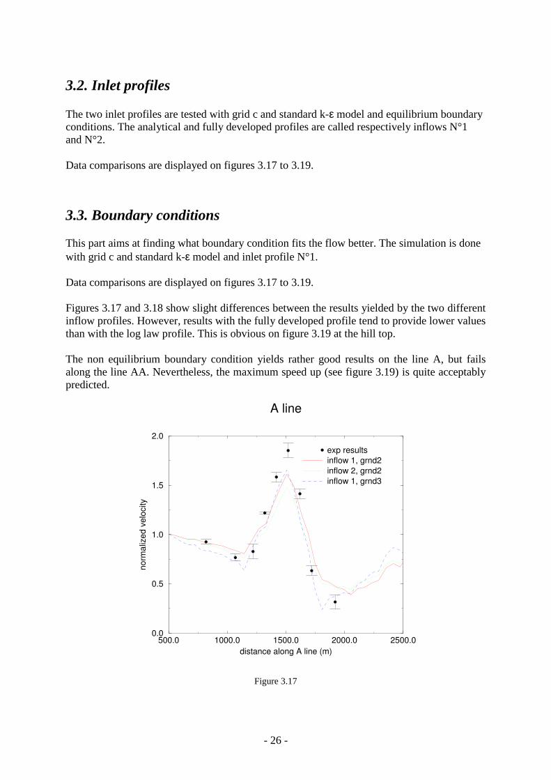
The two inlet profiles are tested with grid c and standard k-ε model and equilibrium boundary conditions. The analytical and fully developed profiles are called respectively inflows N°1 and N°2. Data comparisons are displayed on figures 3.17 to 3.19.

3.3. Boundary conditions This part aims at finding what boundary condition fits the flow better. The simulation is done with grid c and standard k-ε model and inlet profile N°1. Data comparisons are displayed on figures 3.17 to 3.19. Figures 3.17 and 3.18 show slight differences between the results yielded by the two different inflow profiles. However, results with the fully developed profile tend to provide lower values than with the log law profile. This is obvious on figure 3.19 at the hill top. The non equilibrium boundary condition yields rather good results on the line A, but fails along the line AA. Nevertheless, the maximum speed up (see figure 3.19) is quite acceptably predicted.

500.0 1000.0 1500.0 2000.0 2500.0

distance along A line (m)

0.0

0.5

1.0

1.5

2.0

norm

aliz

ed v

elo

city

A line

exp results

inflow 1, grnd2

inflow 2, grnd2

inflow 1, grnd3

Figure 3.17

- 27 -

500.0 1000.0 1500.0 2000.0 2500.0

distance along AA line (m)

0.0

0.5

1.0

1.5

2.0

norm

aliz

ed v

elo

city

AA line

varying inflow

exp results

inflow 1, grnd2

inflow 2, grnd2

inflow 1, grnd3

Figure 3.18

0.0 0.5 1.0 1.5

fractionnal speed up

1

10

100

heig

ht above g

round (

m)

hill top

inflow comparison

exp results

inflow 1, grnd2

inflow 2, grnd2

inflow 1, grnd3

Figure 3.19

- 28 -

PHOTON

DTM - WINDROSE, ANGLE = 270, ID=400

X

Y

UCRT

2.6

3.3

4.0

4.8

5.5

6.2

6.9

7.6

8.3

9.1

9.8

10.5

11.2

11.9

12.6

2.91E+01

Figure 3.17. Inlet profile n°2, GRND2

PHOTON

DTM - WINDROSE, ANGLE = 270, ID=400

X

Y

UCRT

0.7

1.4

2.1

2.8

3.5

4.3

5.0

5.7

6.4

7.1

7.8

8.5

9.3

10.0

10.7

2.71E+01

Figure 3.18. Inlet profile n°1, GRND3

- 29 -

As can be seen on figure 3.17, the inflow n°2 seems not to change the results a lot. On the contrary, the non equilibrium boundary condition seems to yield unphysical solution on the lee side (see figure 3.18). This boundary condition seems not to fit the case.

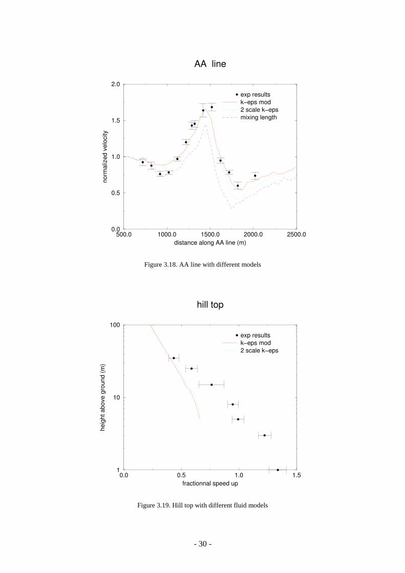
3.4. Turbulence model In this part, different turbulence models are tested : standard k-ε model, modified k-ε model, mixing length model and two-scale k-ε model. The c grid is chosen, boundary condition on the ground is GRND2, inflow is the log law profile.

500.0 1000.0 1500.0 2000.0 2500.0

distance along A line (m)

0.0

0.5

1.0

1.5

2.0

no

rma

lize

d v

elo

city

A line

exp results

k−eps mod

2 scale k−eps

mix length

Figure 3.17. A line with different models

Figures 3.17, 3.18 and 3.19 : The mixing length model yields rather good results along A line but underpredicts velocities along AA line. The modified constants in the k-ε model do not seem to improve the results in comparison with the standard values (is that a mistake in the simulation parameters ?), whereas the two-scale k-ε model, as expected, slightly improves results on the lee side, predicting the same results as the k-ε model upwind the hill top.

- 30 -

500.0 1000.0 1500.0 2000.0 2500.0

distance along AA line (m)

0.0

0.5

1.0

1.5

2.0

no

rma

lize

d v

elo

city

AA line

exp results

k−eps mod

2 scale k−eps

mixing length

Figure 3.18. AA line with different models

0.0 0.5 1.0 1.5

fractionnal speed up

1

10

100

he

igh

t a

bo

ve

gro

un

d (

m)

hill top

exp results

k−eps mod

2 scale k−eps

Figure 3.19. Hill top with different fluid models

- 31 -

PHOTON

DTM - WINDROSE, ANGLE = 270, ID=400

X

Y

UCRT

2.2

2.8

3.4

4.0

4.6

5.2

5.8

6.4

7.0

7.6

8.2

8.8

9.4

10.0

10.6

2.72E+01

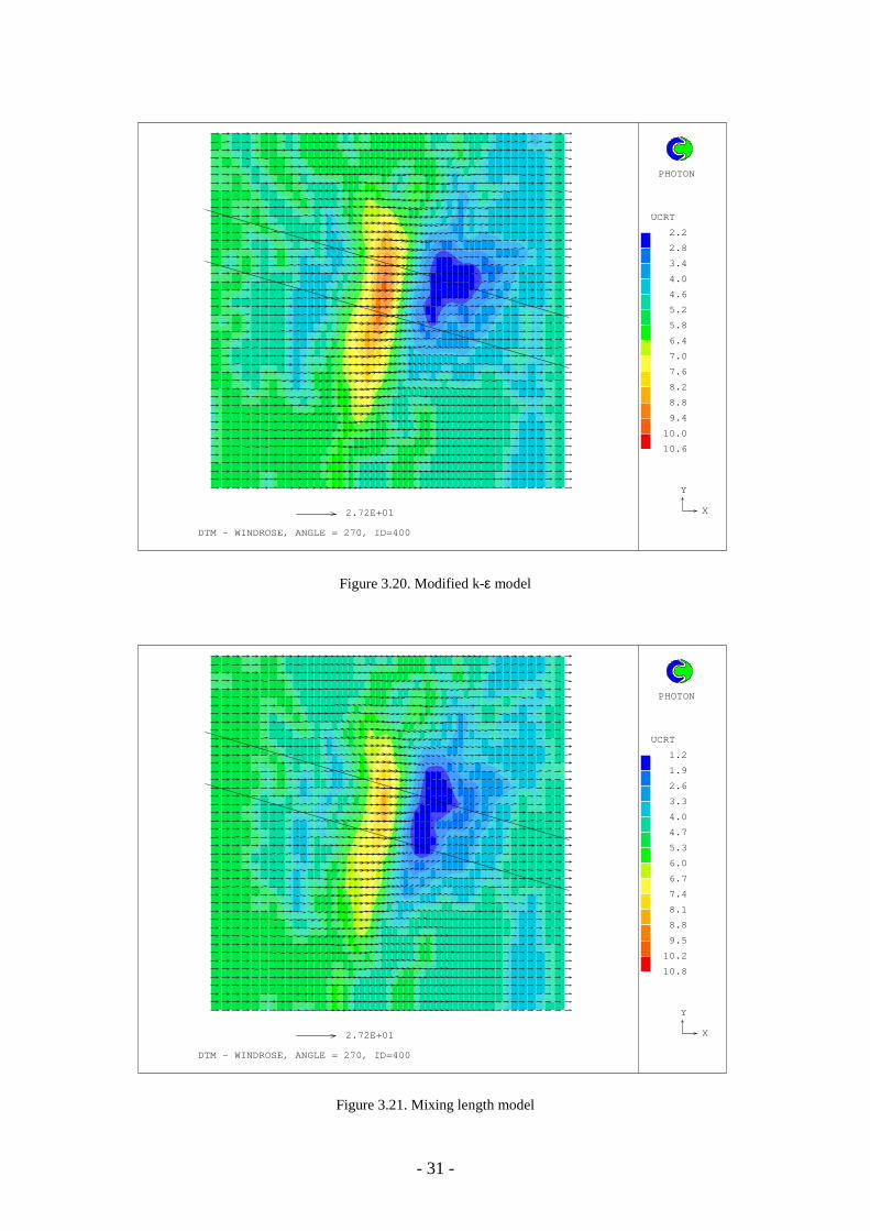
Figure 3.20. Modified k-ε model

PHOTON

DTM - WINDROSE, ANGLE = 270, ID=400

X

Y

UCRT

1.2

1.9

2.6

3.3

4.0

4.7

5.3

6.0

6.7

7.4

8.1

8.8

9.5

10.2

10.8

2.72E+01

Figure 3.21. Mixing length model

- 32 -

PHOTON

DTM - WINDROSE, ANGLE = 270, ID=400

X

Y

UCRT

0.8

1.5

2.2

2.8

3.5

4.2

4.9

5.6

6.3

7.0

7.7

8.3

9.0

9.7

10.4

2.70E+01

Figure 3.22. 2-scale k-ε model

Figures 3.24 and 3.25 show the different speed up profiles at 4 points along line A for both of the standard k-ε model and the two-scale k-ε model. The points are respectively located 400m before HT, HT, 400m after HT and 1000m after HT.

Figure 3.23. Schematic of flow over a hill show different regions of the flow :

inner, middle, outer and wake regions. Source : J.C. KAIMAL and J.J. FINNIGAN, 1994, "Atmospheric Boundary Layer Flows".

Figure 3.23 shows the regions of the flow and explains the shape of vertical profiles at different points on the hill. It should be noted that the wake region has large extension downwind the hill, as it can be seen on the following figures.

- 33 -

−0.20 −0.15 −0.10 −0.05 0.00 0.05

fractionnal speed up

0.0

500.0

1000.0

1500.0

he

igh

t a

bo

ve

gro

un

d (

m)

speed up profiles along line A

−400m

k−eps stand

2 scale k−eps

−0.2 0.0 0.2 0.4 0.6 0.8

fractionnal speed up

0.0

200.0

400.0

600.0

800.0

1000.0

he

igh

t a

bo

ve

gro

un

d (

m)

speed up profiles along line A

hill top

k−eps stand

2 scale k−eps

−0.8 −0.6 −0.4 −0.2 0.0 0.2

fractionnal speed up

0.0

500.0

1000.0

1500.0

heig

ht above g

round (

m)

speed up profiles along line A

+400m

k−eps stand

2 scale k−eps

−0.20 −0.15 −0.10 −0.05 0.00

fractionnal speed up

0.0

500.0

1000.0

1500.0

heig

ht above g

round (

m)

speed up profiles along line A

+1000m

k−eps stand

2 scale k−eps

Figure 3.24. Speed ups comparison -standard k-eps model/2scale k-eps model

at different points along line A

−0.5 0.0 0.5 1.0 1.5

fractionnal speed up

0.0

500.0

1000.0

1500.0

he

igh

t a

bo

ve

gro

un

d (

m)

speed up profiles along line A

grid c

−400 m

ht

+400 m

+1000 m

Figure 3.25. Speed up profiles : standard k-eps model

- 34 -

4. CONCLUDING REMARKS The results from the WindSim code have been tested against experimental data. We saw that the results turn out to be varying a lot according to grid changing. This grid dependency shows the need for grid refinement or improvement. The first cells above the ground are essential to capture the physics of the flow. There is an important gradient in this region. But a too high refinement in z-direction towards the ground causes long thin cells, which may lead to numerical inaccuracy. Therefore a more refined grid in x and y directions should be tested. This can not be done without a digitalisation from a more accurate map of the hill. Exponential distribution, that has not been tested in this study, might improve the results. Unfortunately, the complete results of the Askervein hill experience have not been available for this work. Additional experimental results concerning turbulence quantities could contribute to further analysis of the simulations for this study. This case still raises questions about separation. The question to know whether or not the separation bubble exists is crucial. Such a phenomenon affects the whole velocity field, not only in the separated region. In fact, it seems that separation occurs or almost occurs. Unfortunately, there is not yet simple applicable rules concerning rough wall turbulent separation. The slope of the hill, as well as surface roughness, are sensitive factors for separation. Finnnigan et al (1990) established that for rough cones, a 20 degree slope is the lower limit to ensure steady separation. For the Askervein hill, geometrical parameters have been measured to be approximately H=104 m and L=220 m (see figure), yielding a maximum slope of the order of 14 degrees.

Wind direction H/2 L H/2

Figure 4.1. Normal cross section of the hill with notations If there is separation -and it seems to be virtually the case- how should it be modelled? Is the modelling approach still valid ? Should the assumptions be questioned? Unfortunately, most of information we have about such cases come from mathematical simulations. It should be noted that carrying out experiments in these separated region conditions is not an easy thing to do, since the velocity never reaches its average value. Measurements have though to be carried out on a very large time scale. As emphasised by J.L. Walmsley and P.A. Taylor (1995), pointing out that a lower roughness gives better results for the hill top in a study on the Askervein hill case, there are still questions about the roughness length that should be adopted. A lower roughness seems to give better results for the hill top. Should we adopt a varying roughness model?

- 35 -

It is also stressed in this paper that the velocity field on Askervein may be affected by the neighbouring hills downwind. These hills may probably produce some upwind blockage. (see figure 4.2). Actually, in most cases, the speed on the hill top is underpredicted. This could be related with the fact that the topography around the site is not taken into account. It is assumed to be a flat plain, but even a low hill downwind the Askervein hill could explain that the model provides lower velocities than the measured ones.

Figure 4.2. Contour map of Askervein hill.

Source : P.A. TAYLOR and H.W TEUNISSEN (1986) "The Askervein Hill project : overview and background data"

However, the results are almost as accurate as experimental results, as far uncertainty allows us to judge. Note that as long as wind energy is the matter of interest, the most important point is to predict maximum speed up in the right locations, and, if possible, with good accuracy. The details of flows on the lee side is not relevant for such an application. However, in the interest of micro scale modelling aimed at other purposes-such as pollutant dispersion-, the study of other cases may be desirable.

- 36 -

5. REFERENCES A.R. GRAVDAHL (1998) "Meso scale modelling with a Reynolds Averaged Navier-Stokes solver-Assessment of wind resources along the Norwegian coast", 31st Meeting of experts-State of the art on wind resource estimation, Risø, Denmark October 29-30 1998. Vector, Tønsberg, Norway P.K. CHAVIAROPOULOS and D.I. DOUVIKAS (1998) "Mean-flow-field simulations over complex terrain scale", 31st Meeting of experts-State of the art on wind resource estimation, Risø, Denmark October 29-30 1998. Center for Renewable Energy Sources, Attiki, Greece L.K. ALM and T.A. NYGAARD (1995) "Flow over complex terrain estimated by a general purpose Navier Stokes solver" Institutt for energiteknikk, Kjeller, Norway T. UTNES and K.J. EIDSVIK (1996) "Turbulent flow over mountainous terrain modelled by the Reynolds equations" NTNU, Trondheim, Norway J.C. KAIMAL and J.J. FINNIGAN (1994) "Atmospheric Boundary Layer Flows" Oxford University Press P.A. TAYLOR and H.W TEUNISSEN (1986) "The Askervein Hill project : overview and background data" Atmospheric Environment Service, Downsview, Ontario, Canada K.J. EIDSVIK and T. UTNES (1997) "Flow separation and hydraulic transitions over hills modelled by the Reynolds equations, Journal of wind engineering and industrial aerodynamics" NTNU, Trondheim, Norway H.W. DETERING and D. ETLING (1985) "Application of the E-epsilon model to the atmospheric boundary layer" Institut für Meterologie und Klimatologie, Universität Hannover, Germany D.R. LEMELIN, D. SURRY and A.G. DAVENPORT (1988) "Simple approximations for wind speed-up over hills" Boundary Layer Wind Tunnel Laboratory, University of Western Ontario, London, Canada J.L. WALMSLEY and J. PADRO (1990) "Shear stress results from a mixed spectral finite-difference model : application to the Askervein hill project data" Atmospheric Environment Service, Downsview, Ontario, Canada J.L. WALMSLEY1 and P.A. TAYLOR2 (1995) "Boundary-layer flow over topography : impacts of the Askervein study" 1 : Atmospheric Environment Service, Downsview, Ontario, Canada

- 37 -

2 :Department of Earth Atmospheric Science, York University, Ontario, Canada J.R. SALMON1, A.J. BOWEN2, A.M. HOFF3, R. JOHNSON2, R.E. MICKLE2, P.A. TAYLOR2, G. TETZLAFF3 and J.L. WALMSLEY2 (1987) "The Askervein hill project : mean wind variations at fixed heights above ground" 1 : Contractor, Ontario, Canada 2 : Dept of Mechanical Engineering, University of Canterbury, New Zealand 3 : Institut für Meterologie und Klimatologie, Universität Hannover, Germany F.M. WHITE (1974) "Viscous fluid flow" McGraw-Hill Publishing Company PHOENICS documentation CHAM Ltd