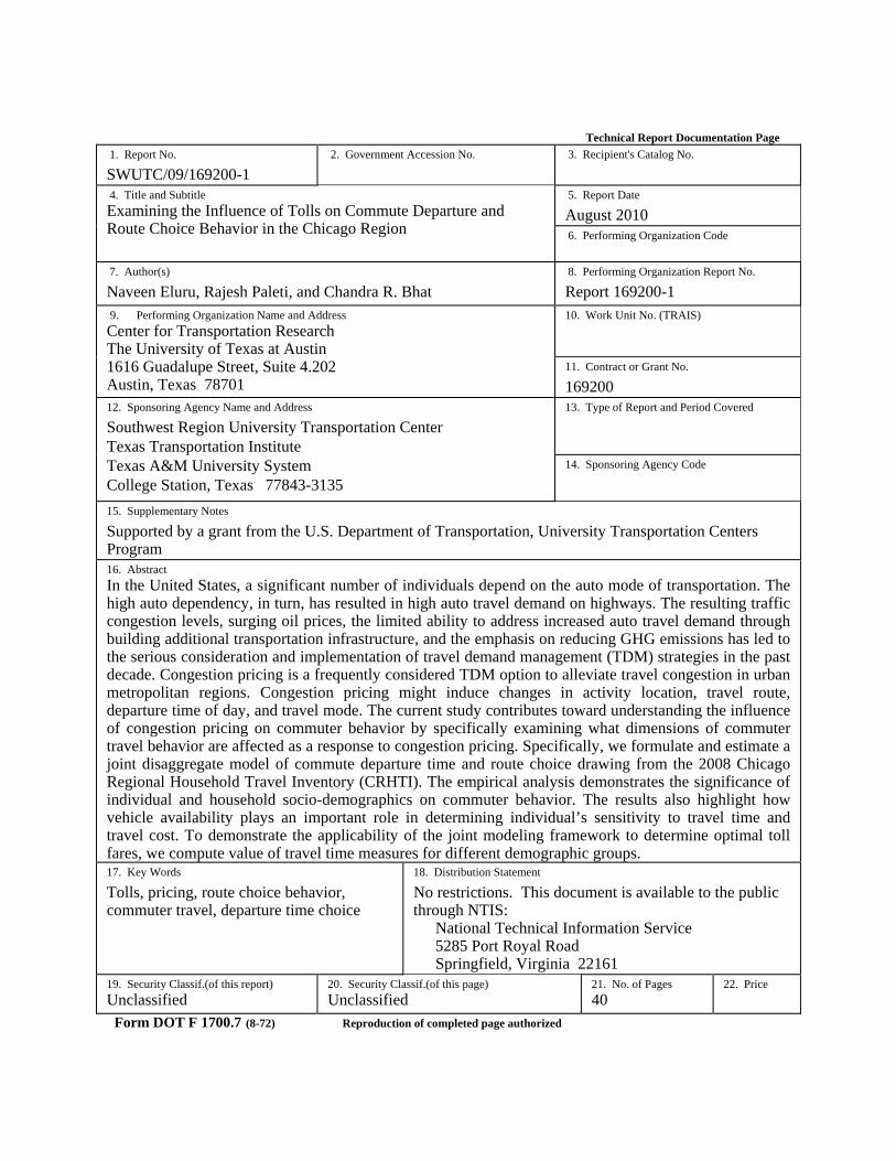
Technical Report Documentation Page 1. Report No.

SWUTC/09/169200-1

2. Government Accession No.

3. Recipient's Catalog No.

4. Title and Subtitle Examining the Influence of Tolls on Commute Departure and Route Choice Behavior in the Chicago Region

5. Report Date

August 2010 6. Performing Organization Code

7. Author(s)

Naveen Eluru, Rajesh Paleti, and Chandra R. Bhat 8. Performing Organization Report No.

Report 169200-1 9. Performing Organization Name and Address Center for Transportation Research The University of Texas at Austin 1616 Guadalupe Street, Suite 4.202 Austin, Texas 78701

10. Work Unit No. (TRAIS)

11. Contract or Grant No.

169200 12. Sponsoring Agency Name and Address

Southwest Region University Transportation Center Texas Transportation Institute Texas A&M University System College Station, Texas 77843-3135

13. Type of Report and Period Covered 14. Sponsoring Agency Code

15. Supplementary Notes

Supported by a grant from the U.S. Department of Transportation, University Transportation Centers Program 16. Abstract In the United States, a significant number of individuals depend on the auto mode of transportation. The high auto dependency, in turn, has resulted in high auto travel demand on highways. The resulting traffic congestion levels, surging oil prices, the limited ability to address increased auto travel demand through building additional transportation infrastructure, and the emphasis on reducing GHG emissions has led to the serious consideration and implementation of travel demand management (TDM) strategies in the past decade. Congestion pricing is a frequently considered TDM option to alleviate travel congestion in urban metropolitan regions. Congestion pricing might induce changes in activity location, travel route, departure time of day, and travel mode. The current study contributes toward understanding the influence of congestion pricing on commuter behavior by specifically examining what dimensions of commuter travel behavior are affected as a response to congestion pricing. Specifically, we formulate and estimate a joint disaggregate model of commute departure time and route choice drawing from the 2008 Chicago Regional Household Travel Inventory (CRHTI). The empirical analysis demonstrates the significance of individual and household socio-demographics on commuter behavior. The results also highlight how vehicle availability plays an important role in determining individual’s sensitivity to travel time and travel cost. To demonstrate the applicability of the joint modeling framework to determine optimal toll fares, we compute value of travel time measures for different demographic groups. 17. Key Words

Tolls, pricing, route choice behavior, commuter travel, departure time choice

18. Distribution Statement

No restrictions. This document is available to the public through NTIS:

National Technical Information Service 5285 Port Royal Road Springfield, Virginia 22161

19. Security Classif.(of this report) Unclassified

20. Security Classif.(of this page) Unclassified

21. No. of Pages 40

22. Price

Form DOT F 1700.7 (8-72) Reproduction of completed page authorized

Examining the Influence of Tolls on Commute Departure and Route Choice Behavior in the Chicago Region

by

Naveen Eluru The University of Texas at Austin

Department of Civil, Architectural and Environmental Engineering

Rajesh Paleti The University of Texas at Austin

Department of Civil, Architectural and Environmental Engineering

and

Dr. Chandra R. Bhat The University of Texas at Austin

Department of Civil, Architectural and Environmental Engineering

Research Report SWUTC/09/169200-1

Southwest Regional University Transportation Center Center for Transportation Research The University of Texas at Austin

Austin, Texas 78712

August 2010

iv

DISCLAIMER The contents of this report reflect the views of the authors, who are responsible for the facts and

the accuracy of the information presented herein. This document is disseminated under the

sponsorship of the Department of Transportation, University Transportation Centers Program in

the interest of information exchange. The U.S. Government assumes no liability for the contents

or use thereof.

v

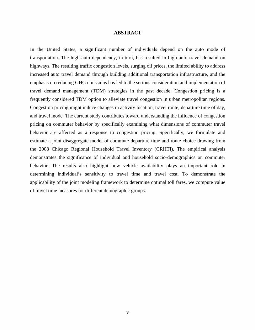
ABSTRACT

In the United States, a significant number of individuals depend on the auto mode of

transportation. The high auto dependency, in turn, has resulted in high auto travel demand on

highways. The resulting traffic congestion levels, surging oil prices, the limited ability to address

increased auto travel demand through building additional transportation infrastructure, and the

emphasis on reducing GHG emissions has led to the serious consideration and implementation of

travel demand management (TDM) strategies in the past decade. Congestion pricing is a

frequently considered TDM option to alleviate travel congestion in urban metropolitan regions.

Congestion pricing might induce changes in activity location, travel route, departure time of day,

and travel mode. The current study contributes toward understanding the influence of congestion

pricing on commuter behavior by specifically examining what dimensions of commuter travel

behavior are affected as a response to congestion pricing. Specifically, we formulate and

estimate a joint disaggregate model of commute departure time and route choice drawing from

the 2008 Chicago Regional Household Travel Inventory (CRHTI). The empirical analysis

demonstrates the significance of individual and household socio-demographics on commuter

behavior. The results also highlight how vehicle availability plays an important role in

determining individual’s sensitivity to travel time and travel cost. To demonstrate the

applicability of the joint modeling framework to determine optimal toll fares, we compute value

of travel time measures for different demographic groups.

vi

ACKNOWLEDGEMENTS

The authors recognize that support for this research was provided by a grant from the U.S.

Department of Transportation, University Transportation Centers Program to the Southwest

Region University Transportation Center.

vii

EXECUTIVE SUMMARY

This research study contributes to the existing literature on congestion pricing by analyzing the

influence of pricing on travel behavior. Specifically, congestion pricing might induce changes in

activity location, travel route, departure time of day, and travel mode. Commuter response to

pricing might involve (1) shifting their departure time interval for both the home-to-work (HW)

and the work-to-home (WH) segments, (2) altering their travel route and (3) shifting from auto

mode to other modes of transportation. In this effort, we investigate the travel route and time of

day choice for commuters who use the auto mode to travel to work. The data used in this study

are drawn from the 2008 Chicago Regional Household Travel Inventory.

The current study examines the commuter departure time interval and travel route

choice in a unified framework. Specifically, the departure time choice alternatives include a joint

combination of time interval of travel for the home-to-work (HW) and the work-to-home (WH)

segments. The travel route alternatives include “toll” and “no toll” routes. The route choice

alternatives are not readily available in the travel data set. So, we manually compiled travel route

characteristics using Google Maps (http://maps.google.com) for travel time information and the

Chicago Toll Calculator for toll fare information

(http://www.getipass.com/tollcalc/TollCalcMain.jsp). The classic multinomial logit model is

employed for the empirical analysis.

The empirical analysis considered several variables to explain departure time and route

choice, including level of service measures (travel time and travel cost measured as toll cost and

operational cost), HW and WH departure interval duration, and interactions of individual

attributes, (age, gender), household socio-demographics (household income, household vehicle

availability computed as number of vehicles per licensed driver), and commuter employment

characteristics (work schedule flexibility) with level of service attributes and departure time

attributes. The results from this exercise provide several insights into commuter behavior. First,

the model results highlight the significance of individual and household demographics on

commute departure choice and travel route choice. Second, individuals, as expected, exhibit an

overall disinclination towards using toll routes for commute unless the toll routes provide a

reasonable travel time savings. Third, female commuters and commuters with high work

flexibility are least likely to choose toll routes for their commute. Finally, the results highlight

the importance of household vehicle availability on commuter route choice. These model

viii

estimation results were employed to compute the implied money value of travel time for

different demographic segments (males, females, high work flexibility etc.) and for different

vehicle availability combinations. The value of time measures point out that commuters with

restricted access to vehicles are less sensitive to travel time compared to commuters with higher

access to vehicles. Further, the value of travel time measurements from the current research

effort allow us to determine the optimal toll pricing schemes for different demographics. The

model framework and the estimation results may be used in environmental justice studies and to

determine toll fares in urban regions.

ix

TABLE OF CONTENTS

CHAPTER 1: INTRODUCTION .................................................................................................1 

1.1  Transportation in the U.S. ...........................................................................................1 1.2  Commuting and Pricing Strategies .............................................................................1 1.3  Studying Commuter Response to Pricing ...................................................................3 

CHAPTER 2: EARLIER STUDIES AND THE CONTEXT OF THE CURRENT STUDY ......5 2.1  Studies Examining Auto-Based Travel Response to Pricing .....................................6 2.2  The Current Study ......................................................................................................7 2.3  Data Considerations ....................................................................................................7 

CHAPTER 3: ANALYSIS FRAMEWORK ................................................................................9 3.1  Departure Time Interval Choice .................................................................................9 3.2  Travel Route Choice .................................................................................................10 3.3  Methodology .............................................................................................................11 

CHAPTER 4: DATA COMPILATION .....................................................................................13 4.1  Data Sources .............................................................................................................13 4.2  Sample Formation and Description ..........................................................................13 4.3  Level of Service Attributes Compilation ..................................................................17 

CHAPTER 5: EMPIRICAL ANALYSIS ...................................................................................19 5.1  Variables Considered ................................................................................................19 5.2  Model Estimation Results .........................................................................................19 

5.2.1 Level of Service Attributes and their Interactions ...........................................20 5.2.2 Departure Time Alternative Characteristics ...................................................21 

5.3  Model Application ....................................................................................................22 5.3.1 Value of Travel Time........................................................................................22 

CHAPTER 6: CONCLUSION ...................................................................................................25 

REFERENCES ...........................................................................................................................27 

x

LIST OF ILLUSTRATIONS

Figure 1. Distribution of WH and HW Commute Departure Times in the Sample .....................15

Table 1. Home to Work and Work to Home Departure Intervals .................................................16

Table 2. Sample Characteristics ....................................................................................................17

Table 3. Estimates of the Joint Departure Time and Travel Route Choice Model .......................20

Table 4. Value of Travel Time Measures .....................................................................................23

4c. Base commuter.............................................................................................................23

4d. Female commuter .........................................................................................................24

4c. Commuter with high flexibility ...................................................................................24

4d. Commuter with high flexibility and household income greater than 100,000 ............24

1

CHAPTER 1: INTRODUCTION

1.1 Transportation in the U.S. In the United States, a significant number of individuals depend on the auto mode of

transportation, in part due to high auto-ownership affordability, inadequate public transportation

facilities (in many cities), and excess suburban land-use developments. The high auto

dependency, in turn, has resulted in high auto travel demand on highways. At the same time, the

ability to build additional infrastructure to meet this growing auto travel demand is limited by

capital costs, real-estate constraints, and environment considerations. The net result is that traffic

congestion levels and air pollution levels in metropolitan areas of the United States have

worsened substantially over the past decade. It is estimated that, in 2007, traffic congestion

resulted in urban residents of the United States traveling 4.2 billion hours longer and purchasing

2.8 billions of extra fuel amounting to a total loss of 87.2 billion dollars to the economy (see

Schrank and Lomax, 2009). Further, the auto-dependency in the U.S. and other developed

countries, combined with the increasing auto-inclination of developing economies, has resulted

in the high demand for oil which, in turn, has led to substantial fluctuations in oil prices that has

adversely affected the economic growth of the United States (Fackler, 2008). Besides, there is

increasing recognition, within the transportation community, that the transportation sector

significantly contributes to Greenhouse Gas (GHG) emissions into the environment. Specifically,

the GHG emissions from the transportation sector in the United States was estimated to account

for about 29% of total GHG emissions in 2006 (EPA, 2006). With the recent emphasis on Global

Climate Change, there is interest within the transportation community and growing political

support to reduce GHG emissions in the U.S. (Burger et al., 2009).

1.2 Commuting and Pricing Strategies Commute-based travel constitutes an important part of transportation travel. The majority of the

work commute travel is undertaken using a private vehicle. In fact, across the US, about 88% of

the commute trips are auto-based (CIA III, 2006). Although, over the years, the fraction of travel

attributable to commute has reduced from 40% of total trips in 1956 to only 16% of total trips in

2000 (CIA III, 2006), commuting still plays a significant role in determining peak travel demand

2

in urban areas. In addition to affecting the peak travel demand, individuals traveling to a work

place also plan significant travel around the work place that affects individuals’ choice of activity

location, route, time and mode of travel. Hence, commuting remains an important element of

overall travel and a significant contributor to peak period traffic congestion in urban areas.

The rising peak period traffic congestion levels, surging oil prices, the limited ability to

address increased auto travel demand through building additional transportation infrastructure,

and the emphasis on reducing GHG emissions has led to the serious consideration and

implementation of peak period travel demand management (TDM) strategies. The main objective

of TDM strategies is to encourage the efficient use of transportation resources by influencing

travel behavior during the peak periods. TDM strategies offer flexible solutions that can be

tailored to meet the specific requirements of a particular urban region.

TDM strategies include: (1) transportation options (such as promoting car sharing,

increased non-motorized connectivity, enhancing existing public transportation services and

building new services such as light rail transit), (2) incentives for reducing auto use and/or

promoting alternate mode use (such as road pricing, entry vehicle charges for central business

districts, promotion schemes for hybrid fuel vehicles, providing park and ride facilities, and

encouraging tele-commuting), and (3) land use strategies (such as neo-urbanist development,

parking pricing, and transit oriented development schemes) (see Litman, 2007 for more details

on TDM strategies). Overall, TDM strategies have the effect of presenting travelers with a

crisper set of commute choices in terms of the attributes characterizing activity location, travel

route, time of day and travel mode alternatives (FHWA, 2008). The implementation of TDM

strategies since 1970s has resulted in a number of studies evaluating how successful these

strategies are in attaining their stated objectives.

Within the context of TDM strategies, congestion pricing is a frequently considered

option to alleviate travel congestion in urban metropolitan regions (FHWA, 2008). Congestion

pricing (also referred to as value pricing) is an economic strategy to shift trips away from

congested routes, congested time periods and the solo-auto mode to less-congested routes, less-

congested time periods, and non-solo auto modes/non-auto modes. Congestion pricing

encompasses different schemes such as cordon tolls, expressway tolls, area-wide charges (for

example entering a central business district), and high occupancy toll lanes (FHWA, 2008).

These schemes, in addition to serving as congestion management tools, also generate revenue by

monetizing the negative externalities associated with the environment and travel times because

3

of congestion. Congestion pricing is prevalent in several states in the U.S. (including California,

Florida, Illinois, Massachusetts, New York, Ohio, Oklahoma, Pennsylvania, Texas, and West

Virginia; see FHWA, 2006a), several countries in Europe (including the United Kingdom,

France, Spain, Italy; see FHWA, 2006b), and other developed and developing countries.

Consequently, there has been substantial research on evaluating the influence of pricing

strategies and tolls on travel behavior.

1.3 Studying Commuter Response to Pricing The current research contributes to the existing literature on congestion pricing by analyzing the

influence of pricing on commute travel behavior. Commuter response to pricing can be rather

complex, and may involve (1) shifting time intervals for departure from home-to-work (HW) and

the time interval for departure from work-to-home (WH), (2) altering the commute travel route,

(3) shifting from auto mode to other modes of transportation, (4) shifting responsibilities for

some activities to other household members, (5) chaining or de-chaining non-work activity stops

from the commute, or combinations of all of these. In addition, in the longer term, commuters

may consider changing work locations and telecommuting. These complex shifts may be

considered in a predictive land-use and activity-based modeling system, though such a system

needs to have an underlying estimated model of commuter behavior. In this effort, we contribute

to such commuter behavioral models by focusing attention on the commuter departure time of

day choice (both to work and from work) and the commuter travel route choice, while assuming

no change to other choices.

Commuter decisions regarding departure time and route choice are a function of

individual work flexibility and travel time for different departure time/travel route combinations.

For instance, an individual with a flexible work schedule has greater freedom in the choice of

departure time. On the other hand, a person with no work flexibility will need to depart to work

well in advance of the work start time to arrive at work prior to the work start time. This decision

also implicitly incorporates a priori knowledge of travel time for the commuter. To illustrate

this, consider that a commuter without work flexibility has a work start time of 8:30 AM. Also,

the commuter has two possible travel routes A and B to arrive at work with travel times of 25

and 35 minutes, respectively. For the home-to-work departure time alternatives prior to 7:55

AM, the commuter has the option of choosing either route A or B. However, for HW departure

time alternatives after 7:55 AM the commuter has the option of route A only. The choice process

4

at hand needs to incorporate this explicitly. Similarly, the WH departure time interval choice

might also be constrained for the commuter based on his/her destination after work. For example,

if the commuter needs to pickup his/her kid from school, the departure time from work is

constrained based on the school end time of the child. In the current study, because we model

departure time and route choice in a joint framework, we are able to accommodate travel

considerations.

To summarize, the choice framework developed in this study simultaneously models the

home-to-work (HW) departure time, the work-to-home (WH) departure time, and the commute

route. The remainder of the report is organized in five sections. Section 2 presents a summary of

earlier literature, discusses implications of available data and positions the current research.

Section 3 describes the modeling methodology employed for the analysis. Section 4 describes the

data compilation effort in detail. Section 5 discusses the empirical results and implications form

the research. Section 6 concludes the report and identifies future directions of research.

5

CHAPTER 2: EARLIER STUDIES AND THE CONTEXT OF THE CURRENT

STUDY There has been considerable research undertaken to examine the influence of congestion pricing

on travel behavior. It is not within the scope of the current research effort to review all these

earlier research. The different aspects related to congestion pricing that have been examined (and

examples of research studies investigating these aspects) include: (1) implementation and

methodological advances of congestion pricing projects (for example see Small and Gomez-

Ibanez, 1998, Lindsey, 2003, Bonsall et al., 2007, Maruyama and Sumalee, 2007, Wichiensin et

al., 2007, Tsekeris and Voß, 2009), (2) feasibility and acceptability of congestion pricing among

road users (for example see Bhattacharjee et al., 1997, Verhoef et al., 1997, Harrington et al.,

2001, King et al., 2007), (3) lessons learned from implementation of congestion pricing projects

(for example see Goh, 2002, Litman, 2006, Santos and Fraser, 2006, Santos, 2008), (4) equity

and welfare cost distribution related to congestion pricing projects (for example see Kitamura et

al., 1999, Parry and Bento, 2001, Lindsey and Verhoef , 2001, Santos and Rojey, 2004, Armelius

and Hultkrantz, 2006, Schweitzer and Taylor, 2008, Ecola and Light, 2009), (5) changes to travel

behavior induced by congestion pricing (for example see Golob, 2001, Bhat and Castelar, 2002,

Brownstone and Small, 2005, Loukopolous et al., 2005, Bhat and Sardesai, 2006, and Hensher

and Puckett, 2007), and (6) transportation network impacts of congestion pricing (for example,

see Yang and Meng, 1998, Kuwahara, 2007, Stewart, 2007).

Among these studies, research efforts that investigate changes in travel behavior as a

result of pricing are of particular relevance to the current study. For instance, Del Mistro et al.,

2007 examined the triggers for changes in different dimensions of travel choice including

residential location, work location, travel mode and departure time. The study involved

descriptive analyses of a retrospective survey that posed questions regarding potential triggers

for changes in each of several choice dimensions. The study found that changes to work place,

change in access to a car, and transportation cost are the primary triggers for changes to travel

behavior. Bhat and Castelar (2002) formulated a mixed logit approach to jointly analyze revealed

and stated preference data. The choice alternatives included mode and time of day combinations.

The authors concluded that congestion pricing during the peak period reduces the likelihood of

6

using drive alone mode during peak periods, and increases off-peak travel, car pooling and travel

by public transportation.

The focus of the aforementioned studies, and several other studies (de Jong et al., 2003,

Bhat and Sardesai, 2006, Washbrook et al., 2006, Hensher and Rose, 2007), has been to compare

and contrast the various characteristics that influence travel mode choice in an effort to

understand how auto-oriented travel behavior can be altered. However, these studies do not

explicitly consider route choice decisions. For example, in an urban region with toll highways,

an individual may choose the auto mode of travel to work, but use a non-toll route to get to work.

The current effort investigates the determinants of such route choice decisions for commuters

using the auto mode of travel. In the rest of this section, we confine our review to studies that

investigate responses in auto-based travel behavior due to pricing.

2.1 Studies Examining Auto-Based Travel Response to Pricing Calfee and Winston (1998), in their research, highlight the need to explicitly consider only auto

alternatives to estimate how much the automobile commuter is willing to pay for reducing travel

time. They employ a stated preference approach to estimate the value of travel time. The authors

concluded that the money value of travel time obtained is low. Loukopolous et al. (2005)

examined possible changes induced in personal vehicle travel in the central business districts due

to congestion pricing. The study observed that introducing congestion pricing would reduce auto

trips, particularly those undertaken by males and low income individuals. Brownstone et al.

(2003) analyzed travel lane choice (characterized as free lanes, car pool lanes and toll lanes)

during peak periods on Interstate Highway 15 to determine the value of travel time for road

users. They report a very high value of travel times of up to 30$/hour. Small and colleagues have

also conducted a host of studies on passenger lane choice (between toll lanes versus free lanes).

Small et al. (2005) applied a joint framework to analyze stated and revealed preference data to

understand the behavior of commuters to choose between toll and non-toll lanes. The study

concluded that road pricing should take advantage of the heterogeneous preferences of travelers

in designing pricing policies by offering travelers with the option of choosing between the toll

and the non-toll option. Brownstone and Small (2005) extended the same framework employed

in Small et al. (2005) to compare results from two road pricing studies. The study found that the

value of time measurement is very close to those estimated in Small et al. (2005). Small et al.

(2006) conducted a study where, in addition to the passenger lane choice, the choice of acquiring

7

an electronic transponder (that permits car users the option to use toll lanes) and the number of

people in their vehicle were modeled.

2.2 The Current Study The preceding discussion provides an overview of earlier research on the influence of pricing on

commuter route (or lane) choice behavior. While these earlier research studies have provided

important insights on commuter responses to pricing, they have not adequately examined joint

decisions regarding travel route choice and departure time choice. Some other earlier studies

have examined the effect of pricing on commuter mode choice (for example, see Bhat and

Sardesai, 2006) or departure time choice (see Noland and Polak, 2002), but these studies also

have not paid attention to the effect of pricing on combinations of choice decisions. The current

study attempts to fill this gap by focusing on the effect of pricing on the joint decision of route

and departure time choice for commute trips. In doing so, we focus only on personal auto trips

and leave the inclusion of mode choice for future research. Further, data constraints lead us to

consider the case of a time-invariant pricing strategy (i.e., tolls). However, note that this does not

negate the value of jointly modeling route and departure time choice, since the choice of whether

to use a tolled route or not is intricately linked to when the commuter would have to depart home

to arrive at work at a certain time (with a certain desired level of reliability). Finally, in the

current study, we consider both the morning commute departure time from home as well as the

evening commute departure time from work, along with route choice, in a joint analysis

framework. This is achieved by formulating and estimating a joint disaggregate model of

commute departure time and route choice, using data from the 2008 Chicago Regional

Household Travel Inventory (CRHTI).

2.3 Data Considerations An important aspect of modeling commuter departure time and route choice travel behavior is

the availability of data for empirical investigation. In practice, it is difficult to obtain data on

route choice. The information on commute travel collected via conventional travel surveys is

generally limited to commute tour departure time intervals (both for the home-to-work or HW

trip, and the work-to-home or WH trip) and travel mode. In some surveys, such as the 2008

Chicago Regional Household Travel Inventory (CRHTI) survey used in the current study,

information on whether the commuter used a toll facility or not is also collected. But, even, in

8

such cases, the actual route alternatives considered by the commuter and the actual route chosen

are not collected. The main reason for not collecting such revealed preference (RP) information

is to avoid burdening the survey respondent and to ensure a reasonable survey response rate.

Some studies by Brownstone and Small (Brownstone et al., 2003, Brownstone and Small, 2005,

Small et al., 2005, and Small et al., 2006) have used RP data, but have focused on a specific

highway segment on which both toll and non-toll options are available to undertake a choice

analysis for users of the highway segment. However, this approach is rather restrictive and

cannot be employed to study response to congestion pricing in urban regions as a whole. The

approach is also unable to examine other dimensions of choice such as time-of-day choice.

Another alternative data collection strategy to examine pricing effects is based on stated

preference (SP) data, where respondents are presented with carefully controlled and designed

“priced” and non-priced” alternatives and asked to choose a particular alternative. SP data have

their own advantages and limitations vis-à-vis RP data sources. For instance, since SP exercises

provide respondents with the attributes of alternative competing routes, and ask respondents to

choose their preferred route, the resulting data immediately enables route choice modeling.

However, SP data collection methods can suffer from “non-reality” effects, since the choices are

being made in a hypothetical context rather than in a real decision-making context.

In this research, we use RP data, but supplement the RP data with route generation

procedures (including tolled and non-tolled routes) based on the home and work locations of

commuters (as we indicate later, we focus attention only on those commuters who travel directly

to work from home without any intermediate stops and who return home in the evening from

work without any intermediate stops). Then, since the 2008 Chicago Regional Household Travel

Inventory (CRHTI) survey did collect information on whether a toll or a non-toll route was used

by the commuter, we are able to combine the route generation exercise with a choice of route to

estimate a joint departure time-route choice model for the commute.

9

CHAPTER 3: ANALYSIS FRAMEWORK

In the current section, we discuss the framework employed to study how commuters respond to

toll pricing in the Chicago region. Prior to detailing the actual framework, we outline the

assumptions in formulating the study framework. First, in developing the commuter tour

departure time interval and route choice model, we consider the typical daily work start and end

time as being exogenously determined. Most activity based frameworks model daily work

departure time choice subsequent to determining typical work start and end times (see for

example Bhat et al., 2004). Second, we limit ourselves to commuters who travel from home-to-

work and back without any intermediate stops. This is done to make the route generation effort

manageable, given the home and work locations of each commuter. Specifically, in the current

study, the generation of travel level of service information for each commuter was manually

undertaken based on information from Google Maps. If we consider commuters with

intermediate stops during the commute, the level of this manual effort increases quite

substantially. At the same time, about half of the commuters in the Chicago region are observed

to commute without any stops. Thus, we focus on this fraction of the commuting population,

setting aside a more extensive analysis of other commuters for a future study.

As indicated earlier in the report, the choices examined in this research include the

commute departure time interval choice (for home-to-work (HW) and work-to-home (WH)

segments) and travel route choice. Each of these choice dimensions is discussed in turn in the

subsequent sections.

3.1 Departure Time Interval Choice The departure time choice interval alternatives include a joint combination of time interval of

travel for the home-to-work (HW) and the work-to-home (WH) segments. To develop the

discrete departure time alternatives, the day is classified into M discrete time periods for the HW

segment departure time, and N discrete time periods for the WH segment departure time,

resulting in a total of M*N possible departure time alternatives. To determine the feasibility of

these M*N possible alternatives for each commuter, we employed information on the typical

work day information (includes work flexibility, work start time, work end time, and work

10

duration) collected from respondents in the Chicago survey. The work flexibility information is

collected in three categories: (a) no flexibility, (b) medium flexibility and (c) high flexibility. For

individuals without any work flexibility, departure time alternatives for the HW trip that permit

the commuter to arrive prior to the typical work start time and departure time alternatives for the

WH trip that are after the typical work end time are considered feasible. For individuals with

medium work flexibility, commuters are allowed to arrive at work later, up to within 2 intervals

of their typical workday schedule. Similarly, these commuters are also allowed to end their work

2 intervals earlier than their typical work schedules. For individuals with high work flexibility,

all HW and WH departure time alternatives are available. The feasible alternatives obtained

based on the worker flexibility constraints are subsequently subjected to the work duration

constraint. Of the feasible combinations based on work flexibility and work start/end times, only

alternatives with work duration greater than the typical work duration are considered feasible.

For example, consider the case where 9:00 AM – 9:15 AM is a possible HW departure

alternative and 2:00 PM – 2:15 PM is a possible WH departure alternative, based on work

flexibility and work start/end times. The work duration for this alternative combination is

approximately 5 hours. However, if the commuter in consideration has a typical work duration of

8 hours, the alternative described above is infeasible. In this manner, there are bound to be

several infeasible combinations (say K) from the possible MN alternatives, resulting in (MN–K)

feasible alternatives for the joint departure time choice dimension. The reader would note that

the number of infeasible alternatives for each commuter is clearly a function of his/her work

flexibility, work duration information, and travel time to work on toll and non-toll routes. This is

where the route choice component becomes important, since the feasible alternatives for

departure time (and the actual chosen departure time alternative) would be a function of whether

a toll route or a non-toll route is chosen.

3.2 Travel Route Choice The generation of alternatives for examining route choice behavior is not straightforward. In

traditional household surveys, the analyst has detailed information only on the origin and

destination of each trip, though the Chicago survey includes information on whether a tolled

facility was used or not for each trip. So, for examining route choice behavior, the analyst needs

to generate possible competing alternatives. Within a transportation network, generating all

possible routes (and their attributes) between a commuter’s home and work locations is

11

infeasible. In the current study, we generated two routes for each commuter. These are: (1) the

best non-toll route between the commuter’s home and work locations and (2) the best toll route

between the commuter’s home and work locations. To determine the optimal toll and non-toll

routes between each home and work location pair, we used Google Maps. For all commuters, the

optimal non-toll and toll routes were not substantially different for the HW and WH segments.

So, we considered the same toll and non-toll routes for both these segments, and generated two

possible routes for the entire commute tour. After the information was compiled, the joint choice

set was obtained by combining the travel route choice dimension with departure time choice

dimension. The overall joint choice model has (MN–K)*2 choice alternatives. The chosen

departure time-route alternative is based on the observed departure times and the indication of

the commuter whether or not s/he chose a tolled route during the commute.

3.3 Methodology A simple classical Multinomial Logit (MNL) model is employed to examine the joint choice of

commute departure time and route choice. The modeling framework is briefly presented in this

section. Let q be the index for commuters (q = 1, 2, ..., Q) and i be the index for the possible

combinations of departure time and travel route choice (i = 1, 2, ..., (MN–K)*2). With this

notation, the random utility formulation takes the following familiar form:

* 'qi qi qiu xβ ε= + (1)

In the above equation, *qiu represents the utility obtained by the qth commuter in choosing the ith

alternative. qix is a column vector of attributes including: (1) level of service attributes (such as

travel time and travel cost), (2) departure time interval characteristics (such as duration length of

the interval), (3) interactions of individual and household socio-demographics (sex of individual,

presence of children, etc.) with the above two categories, and (4) interactions of employment

characteristics with the first two categories. β is a corresponding coefficient column vector of

parameters to be estimated, and qiε is an idiosyncratic error term assumed to be standard type-1

extreme value distributed. Then, in the usual spirit of utility maximization, commuter q will

choose the alternative that offers the highest utility. The probability expression for choosing

alternative i is given by:

12

exp( ' )

exp( ' )qi

qiqi

i

xP

xββ

=∑

(2)

The log-likelihood function is constructed based on the above probability expression, and

maximum likelihood estimation is employed to estimate the β parameter.

13

CHAPTER 4: DATA COMPILATION

4.1 Data Sources The data used in this study are drawn from the 2008 Chicago Regional Household Travel

Inventory (CRHTI), which was sponsored by the Chicago Metropolitan Agency for Planning

(CMAP), the Illinois Department of Transportation (IDOT), the Northwestern Indiana Regional

Planning Commission, and the Indiana Department of Transportation. The study area for the

survey included eight counties in Illinois (Cook, DuPage, Grundy, Kane, Kendall, Lake,

McHenry, and Will counties), and three counties in Indiana (Lake, LaPorte, and Porter). The

survey was administered using standard postal mail-based survey methods and computer-aided

telephone interview (CATI) technology through Travel Tracker Survey to facilitate the

organization and storage of the data. For details of the survey design and implementation

methods, the reader is referred to NuStats (2008). The primary objective of the survey was to

collect data to aid the development of regional travel demand models for the Chicago region. The

survey collected information on the activity and travel information for all household members

(regardless of age) during a randomly assigned 1-day or 2-day period (the 1-day period sample

focused only on weekdays, while the 2-day period sample targeted two consecutive days

including the Sunday/Monday and Friday/Saturday pairs but not the Saturday/Sunday pair).

Further, the survey respondents were also requested to provide information on household

demographics and individual demographics of each household member, household vehicle

ownership, employment characteristics, and geo-coded residence and work locations. The survey

also collected information regarding toll road usage and corresponding toll fare for every travel

episode.

4.2 Sample Formation and Description The activity and travel information collected in the survey formed the basis of the empirical

analysis. The data assembly process involved the following steps. First, employed individuals

were identified and their work travel patterns were screened for detailed analysis. Second, of the

employed individuals, workers who used the auto mode for their commute travel were selected.

Third, among the auto commuters, individuals who traveled directly to work from home and

14

vice-versa were identified. Fourth, household and individual attributes, geo-coded residential and

work location, and toll road usage and toll fare charges for these selected commuters were

appended to the dataset. Fifth, the dataset obtained was checked for consistency and records with

missing and/or inaccurate information were deleted. Sixth, the time periods for the HW and WH

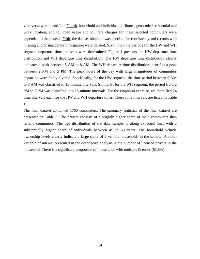
segment departure time intervals were determined. Figure 1 presents the HW departure time

distribution and WH departure time distribution. The HW departure time distribution clearly

indicates a peak between 5 AM to 8 AM. The WH departure time distribution identifies a peak

between 2 PM and 5 PM. The peak hours of the day with large magnitudes of commuters

departing were finely divided. Specifically, for the HW segment, the time period between 5 AM

to 8 AM was classified in 15-minute intervals. Similarly, for the WH segment, the period from 2

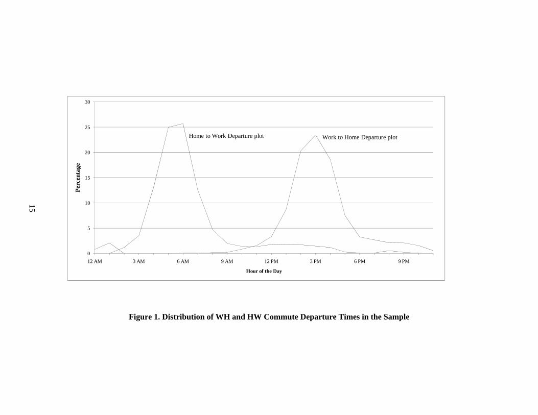
PM to 5 PM was classified into 15-minute intervals. For the empirical exercise, we identified 24

time intervals each for the HW and WH departure times. These time intervals are listed in Table

1.

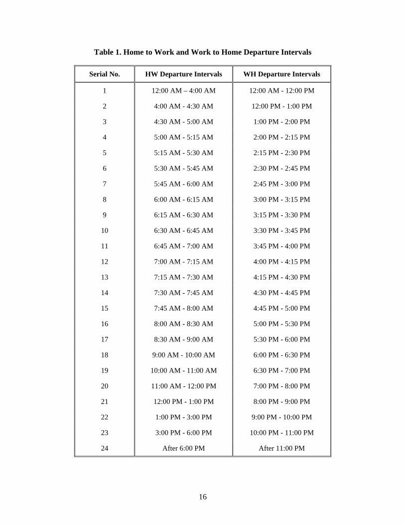
The final dataset contained 1760 commuters. The summary statistics of the final dataset are

presented in Table 2. The dataset consists of a slightly higher share of male commuters than

female commuters. The age distribution of the data sample is along expected lines with a

substantially higher share of individuals between 45 to 60 years. The household vehicle

ownership levels clearly indicate a large share of 2 vehicle households in the sample. Another

variable of interest presented in the descriptive analysis is the number of licensed drivers in the

household. There is a significant proportion of households with multiple licenses (82.8%).

0

5

10

15

20

25

30

12 AM 3 AM 6 AM 9 AM 12 PM 3 PM 6 PM 9 PM

Perc

enta

ge

Hour of the Day

Home to Work Departure plot Work to Home Departure plot

Figure 1. Distribution of WH and HW Commute Departure Times in the Sample

15

16

Table 1. Home to Work and Work to Home Departure Intervals

Serial No. HW Departure Intervals WH Departure Intervals

1 12:00 AM – 4:00 AM 12:00 AM - 12:00 PM

2 4:00 AM - 4:30 AM 12:00 PM - 1:00 PM

3 4:30 AM - 5:00 AM 1:00 PM - 2:00 PM

4 5:00 AM - 5:15 AM 2:00 PM - 2:15 PM

5 5:15 AM - 5:30 AM 2:15 PM - 2:30 PM

6 5:30 AM - 5:45 AM 2:30 PM - 2:45 PM

7 5:45 AM - 6:00 AM 2:45 PM - 3:00 PM

8 6:00 AM - 6:15 AM 3:00 PM - 3:15 PM

9 6:15 AM - 6:30 AM 3:15 PM - 3:30 PM

10 6:30 AM - 6:45 AM 3:30 PM - 3:45 PM

11 6:45 AM - 7:00 AM 3:45 PM - 4:00 PM

12 7:00 AM - 7:15 AM 4:00 PM - 4:15 PM

13 7:15 AM - 7:30 AM 4:15 PM - 4:30 PM

14 7:30 AM - 7:45 AM 4:30 PM - 4:45 PM

15 7:45 AM - 8:00 AM 4:45 PM - 5:00 PM

16 8:00 AM - 8:30 AM 5:00 PM - 5:30 PM

17 8:30 AM - 9:00 AM 5:30 PM - 6:00 PM

18 9:00 AM - 10:00 AM 6:00 PM - 6:30 PM

19 10:00 AM - 11:00 AM 6:30 PM - 7:00 PM

20 11:00 AM - 12:00 PM 7:00 PM - 8:00 PM

21 12:00 PM - 1:00 PM 8:00 PM - 9:00 PM

22 1:00 PM - 3:00 PM 9:00 PM - 10:00 PM

23 3:00 PM - 6:00 PM 10:00 PM - 11:00 PM

24 After 6:00 PM After 11:00 PM

17

Table 2. Sample Characteristics

Variable Sample shares

Gender Female 44.7 Male 55.3

Age categories 16-30 years 15.6 30-45 years 30.9 45-60 years 42.8 > 60 years 10.7

Number of Vehicles in the household 1 vehicle 18.2 2 vehicles 52.4 3 vehicles 20.6 4 or more vehicles 8.8

Number of licensed individuals in the household One 17.2 Two 58.9 Three or more 23.9

4.3 Level of Service Attributes Compilation As previously discussed, any revealed preference dataset contains information only on the

chosen alternatives i.e. for commuter opting for the “no toll” route the “toll” route information is

unavailable and vice-versa. The examination of the choice behavior necessitates generation of

information regarding other alternatives in the choice set. To do so, we need to obtain, for every

commuter, the travel time and travel cost for the optimal “no toll” and “toll” routes. For this

purpose, we used Google Maps web application to identify the two optimal routes and obtained

detailed level of service information (http://maps.google.com). Google Maps allows us to

generate potential travel routes by providing as input the geo-coded home and work locations

(latitude and longitude). In fact, the website provides up to three alternate routes for each origin

and destination. Under the default settings, Google Maps provides us the shortest route to the

destination by time. The application allows us to opt for “no toll” routes via the “avoid toll”

18

option that allows the identification of the shortest “no toll” option. For some commuters in the

dataset, it is possible that a “toll” route might not exist.

The level of service information provided by Google maps includes travel time

information during uncongested and congested time periods.1 In the current study, this

information was used to obtain travel times for peak and off-peak periods.2 However, the

website does not provide the toll cost for the “toll” routes. For this purpose, we used the Chicago

Toll Calculator (http://www.getipass.com/tollcalc/TollCalcMain.jsp). The Toll Calculator tool

allows the computation of the toll cost by the entry and exit points by vehicle type on all major

toll routes in the Chicago region. So, in this study effort, we manually identified the toll route

entry and exit points from the Google maps travel route and computed the toll cost from the

Calculator tool. The level of service information generated in this form was appropriately

appended to the commuter’s characteristics. Specifically, the level of service information

collected via Google Maps and Chicago Toll calculator is collated to obtain the total travel time

and travel cost for each HW, WH and travel route (“toll” versus “no toll”) combination. In this

process, and based on the time periods of the HW and WH segments, appropriate peak or non-

peak travel times were included in the travel time computation. The toll cost for each of the

alternative combinations does not vary for peak and off-peak periods because the Chicago city

employs a time invariant toll pricing scheme.

1 Google Maps does not explicitly provide information on the time of day for the congested travel. In this study, we assume that the congested travel occurs during the peak periods. 2 For this study, the 6 am to 9 am and 3 pm to 6 pm periods were considered peak travel periods.

19

CHAPTER 5: EMPIRICAL ANALYSIS

5.1 Variables Considered Several variables including level of service measures (travel time and travel cost for toll and

operational cost), HW and WH departure interval duration, and interactions of individual

attributes (age, gender), household socio-demographics (household income, household vehicle

availability computed as number of vehicles per licensed driver), and commuter employment

characteristics (work schedule flexibility) with level of service attributes and departure time

interval attributes were considered. The estimation effort involved the selection of variables and

their interactions based on prior research, removing statistically insignificant variables, and

combining variable effects when they were not statistically different from each other. Further, for

the continuous variables in the data (such as age), we tested different alternative functional forms

that included a linear form, a spline (or piece-wise linear) form, and dummy variables for

different ranges.

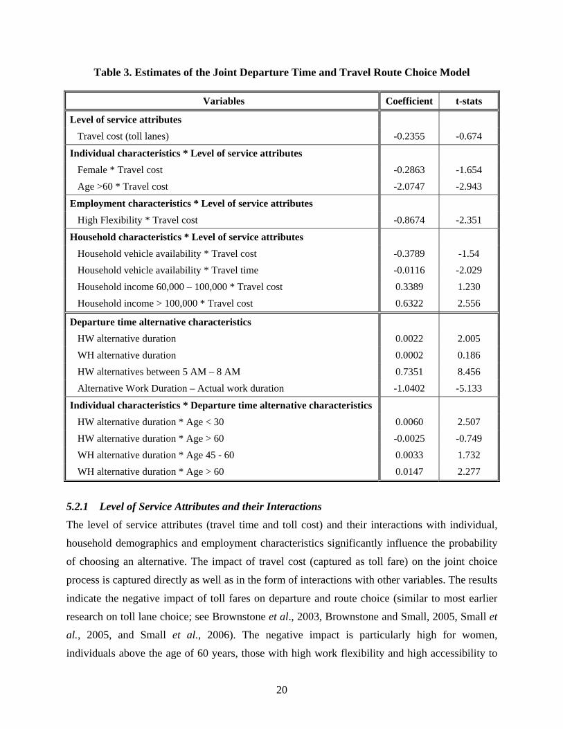
5.2 Model Estimation Results Table 3 provides the results of the MNL model. In the current research effort, the coefficient on

operational cost was statistically insignificant. We examined various interactions and different

plausible functional forms for the operation cost variable in the specification, but it consistently

turned out to be statistically insignificant. So, the travel cost variable used in the final

specification corresponds only to the toll fare.

The results of the joint departure time and travel route choice model are discussed in the

subsequent sections.

20

Table 3. Estimates of the Joint Departure Time and Travel Route Choice Model

Variables Coefficient t-stats

Level of service attributes Travel cost (toll lanes) -0.2355 -0.674

Individual characteristics * Level of service attributes Female * Travel cost -0.2863 -1.654 Age >60 * Travel cost -2.0747 -2.943

Employment characteristics * Level of service attributes High Flexibility * Travel cost -0.8674 -2.351

Household characteristics * Level of service attributes Household vehicle availability * Travel cost -0.3789 -1.54 Household vehicle availability * Travel time -0.0116 -2.029 Household income 60,000 – 100,000 * Travel cost 0.3389 1.230 Household income > 100,000 * Travel cost 0.6322 2.556

Departure time alternative characteristics HW alternative duration 0.0022 2.005 WH alternative duration 0.0002 0.186 HW alternatives between 5 AM – 8 AM 0.7351 8.456 Alternative Work Duration – Actual work duration -1.0402 -5.133

Individual characteristics * Departure time alternative characteristics HW alternative duration * Age < 30 0.0060 2.507 HW alternative duration * Age > 60 -0.0025 -0.749 WH alternative duration * Age 45 - 60 0.0033 1.732 WH alternative duration * Age > 60 0.0147 2.277

5.2.1 Level of Service Attributes and their Interactions

The level of service attributes (travel time and toll cost) and their interactions with individual,

household demographics and employment characteristics significantly influence the probability

of choosing an alternative. The impact of travel cost (captured as toll fare) on the joint choice

process is captured directly as well as in the form of interactions with other variables. The results

indicate the negative impact of toll fares on departure and route choice (similar to most earlier

research on toll lane choice; see Brownstone et al., 2003, Brownstone and Small, 2005, Small et

al., 2005, and Small et al., 2006). The negative impact is particularly high for women,

individuals above the age of 60 years, those with high work flexibility and high accessibility to

21

vehicles, and individuals in low income households (note that the household vehicle availability

variable is computed as the ratio of the number of household vehicles to the number of licensed

drivers in the commuter’s household; this variable provides an indication of how accessible a

vehicle is to the commuter). That is, women, older commuters, individuals with high work

flexibility and high vehicle access, and low income individuals are less likely to use the toll road

alternative relative to their peers.

The travel time effect indicates that commuters with higher access to vehicles are more

sensitive to travel time.

5.2.2 Departure Time Alternative Characteristics

The departure time interval alternative characteristics, as expected, affect commuter travel

behavior. As expected, the likelihood of choosing the HW and WH interval alternatives is

directly proportional to the interval duration (see Guo et al., 2005 for a similar result in work

start and end time modeling). Further, the results indicate a strong general propensity to choose a

HW departure between time periods 5 AM to 8 AM. The result clearly highlights commuters’

preference towards starting work early in the day. These findings are consistent with commuting

facts reported by Commuting in America report (CIA III, 2006). Another result of significant

interest from this group of variables is the influence of the difference in commuter work duration

for the chosen alternative and the commuter’s typical work duration. The result indicates that

commuters opt for HW and WH departure times such that the resulting work duration is not

substantially different from their typical work duration.

Within the departure time interval alternative characteristics, only the interactions with

individual characteristics affect commuter choice behavior. In particular, the interactions of

departure time interval with age of the commuter are statistically significant. Specifically,

commuters aged less than 30 years are positively influenced by HW departure interval duration

compared to commuters aged between 30 and 60 years. However, commuters aged more than 60

years exhibit lower proclivity to be affected by HW departure interval duration. Interactions of a

similar nature for the WH departure intervals yield slightly different results. These findings

indicate that commuters aged more than 45 years are positively influenced by alternative interval

duration with the effect being even more pronounced for older commuters (age >60).

22

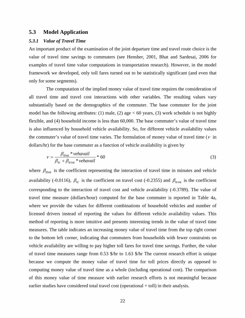
5.3 Model Application 5.3.1 Value of Travel Time

An important product of the examination of the joint departure time and travel route choice is the

value of travel time savings to commuters (see Hensher, 2001, Bhat and Sardesai, 2006 for

examples of travel time value computations in transportation research). However, in the model

framework we developed, only toll fares turned out to be statistically significant (and even that

only for some segments).

The computation of the implied money value of travel time requires the consideration of

all travel time and travel cost interactions with other variables. The resulting values vary

substantially based on the demographics of the commuter. The base commuter for the joint

model has the following attributes: (1) male, (2) age < 60 years, (3) work schedule is not highly

flexible, and (4) household income is less than 60,000. The base commuter’s value of travel time

is also influenced by household vehicle availability. So, for different vehicle availability values

the commuter’s value of travel time varies. The formulation of money value of travel time (ν in

dollars/hr) for the base commuter as a function of vehicle availability is given by

**

ttva

tc tcva

vehavailvehavail

βν

β β=

+* 60 (3)

where ttvaβ is the coefficient representing the interaction of travel time in minutes and vehicle

availability (-0.0116), tcβ is the coefficient on travel cost (-0.2355) and tcvaβ is the coefficient

corresponding to the interaction of travel cost and vehicle availability (-0.3789). The value of

travel time measure (dollars/hour) computed for the base commuter is reported in Table 4a,

where we provide the values for different combinations of household vehicles and number of

licensed drivers instead of reporting the values for different vehicle availability values. This

method of reporting is more intuitive and presents interesting trends in the value of travel time

measures. The table indicates an increasing money value of travel time from the top right corner

to the bottom left corner, indicating that commuters from households with fewer constraints on

vehicle availability are willing to pay higher toll fares for travel time savings. Further, the value

of travel time measures range from 0.53 $/hr to 1.63 $/hr The current research effort is unique

because we compute the money value of travel time for toll prices directly as opposed to

computing money value of travel time as a whole (including operational cost). The comparison

of this money value of time measure with earlier research efforts is not meaningful because

earlier studies have considered total travel cost (operational + toll) in their analysis.

23

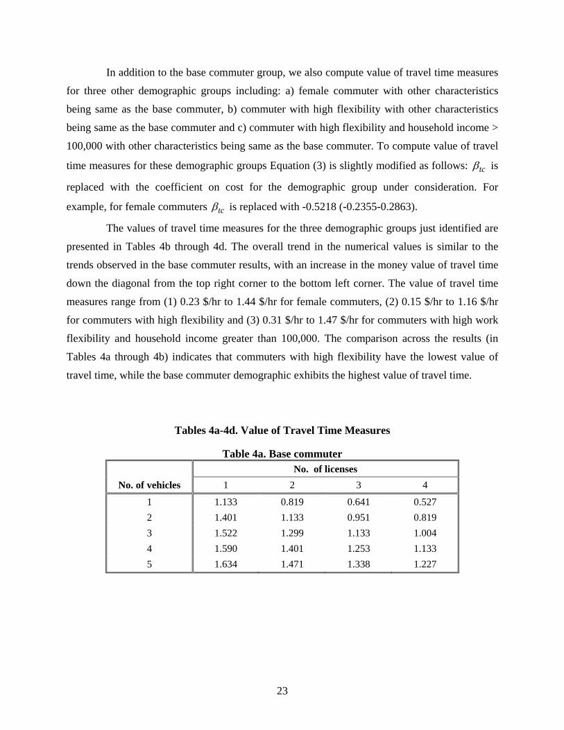
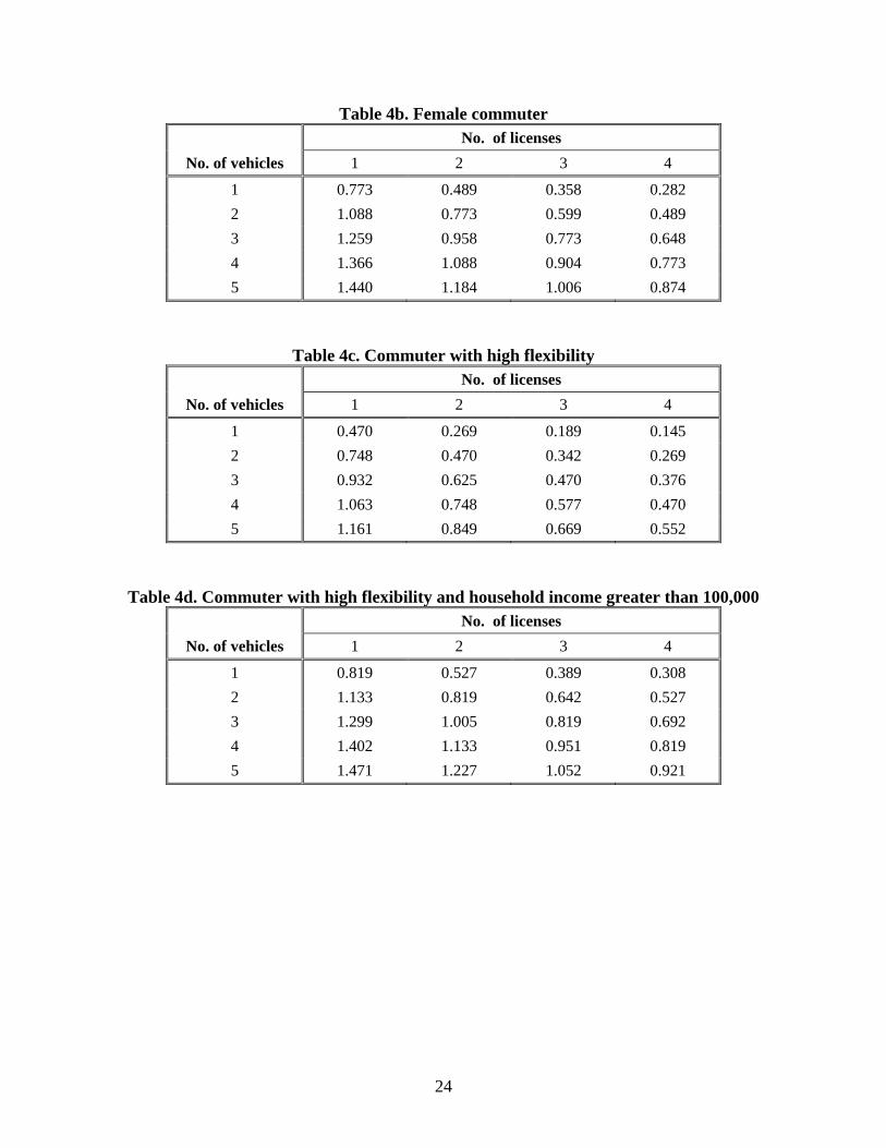
In addition to the base commuter group, we also compute value of travel time measures

for three other demographic groups including: a) female commuter with other characteristics

being same as the base commuter, b) commuter with high flexibility with other characteristics

being same as the base commuter and c) commuter with high flexibility and household income >

100,000 with other characteristics being same as the base commuter. To compute value of travel

time measures for these demographic groups Equation (3) is slightly modified as follows: tcβ is

replaced with the coefficient on cost for the demographic group under consideration. For

example, for female commuters tcβ is replaced with -0.5218 (-0.2355-0.2863).

The values of travel time measures for the three demographic groups just identified are

presented in Tables 4b through 4d. The overall trend in the numerical values is similar to the

trends observed in the base commuter results, with an increase in the money value of travel time

down the diagonal from the top right corner to the bottom left corner. The value of travel time

measures range from (1) 0.23 $/hr to 1.44 $/hr for female commuters, (2) 0.15 $/hr to 1.16 $/hr

for commuters with high flexibility and (3) 0.31 $/hr to 1.47 $/hr for commuters with high work

flexibility and household income greater than 100,000. The comparison across the results (in

Tables 4a through 4b) indicates that commuters with high flexibility have the lowest value of

travel time, while the base commuter demographic exhibits the highest value of travel time.

Tables 4a-4d. Value of Travel Time Measures

Table 4a. Base commuter No. of licenses

No. of vehicles 1 2 3 4

1 1.133 0.819 0.641 0.527 2 1.401 1.133 0.951 0.819 3 1.522 1.299 1.133 1.004 4 1.590 1.401 1.253 1.133 5 1.634 1.471 1.338 1.227

24

Table 4b. Female commuter No. of licenses

No. of vehicles 1 2 3 4

1 0.773 0.489 0.358 0.282 2 1.088 0.773 0.599 0.489 3 1.259 0.958 0.773 0.648 4 1.366 1.088 0.904 0.773 5 1.440 1.184 1.006 0.874

Table 4c. Commuter with high flexibility No. of licenses

No. of vehicles 1 2 3 4

1 0.470 0.269 0.189 0.145 2 0.748 0.470 0.342 0.269 3 0.932 0.625 0.470 0.376 4 1.063 0.748 0.577 0.470 5 1.161 0.849 0.669 0.552

Table 4d. Commuter with high flexibility and household income greater than 100,000 No. of licenses

No. of vehicles 1 2 3 4

1 0.819 0.527 0.389 0.308 2 1.133 0.819 0.642 0.527 3 1.299 1.005 0.819 0.692 4 1.402 1.133 0.951 0.819 5 1.471 1.227 1.052 0.921

25

CHAPTER 6: CONCLUSION

In the United States, a significant number of individuals depend on the auto mode of

transportation, in part due to high auto-ownership affordability, inadequate public transportation

facilities (in many cities), and excess suburban land-use developments. The high auto

dependency, in turn, has resulted in high auto travel demand on highways leading to increased

traffic congestion levels and air pollution levels in metropolitan areas of United States. Further,

with the recent emphasis on Global Climate Change, there is increasing interest within the

transportation community and growing political support to reduce GHG emissions in the U.S.

The rising traffic congestion levels, surging oil prices, the limited ability to address increased

auto travel demand through building additional transportation infrastructure, and the emphasis on

reducing GHG emissions has led to the serious consideration and implementation of travel

demand management (TDM) strategies in the past decade. Within the context of TDM strategies,

congestion pricing is a frequently considered option to alleviate travel congestion in urban

metropolitan regions. The current research contributes to the existing literature on congestion

pricing by analyzing the influence of pricing on travel behavior. Specifically, congestion pricing

might induce changes in activity location, travel route, departure time of day, and travel mode.

Commuter response to pricing might involve (1) shifting their departure time interval for both

the home-to-work (HW) and the work-to-home (WH) segments, (2) altering their travel route

and (3) shifting from auto mode to other modes of transportation. In this effort, we investigate

the travel route and time of day choice for commuters who use the auto mode to travel to work.

The data used in this study are drawn from the 2008 Chicago Regional Household Travel

Inventory.

The current study examines the commuter departure time interval and travel route

choice in a unified framework. Specifically, the departure time choice alternatives include a joint

combination of time interval of travel for the home-to-work (HW) and the work-to-home (WH)

segments. The travel route alternatives include “toll” and “no toll” routes. The route choice

alternatives are not readily available in the travel data set. So, we manually compiled travel route

characteristics using Google Maps (http://maps.google.com) for travel time information and the

Chicago Toll Calculator for toll fare information

26

(http://www.getipass.com/tollcalc/TollCalcMain.jsp). The classic multinomial logit model is

employed for the empirical analysis.

The empirical analysis considered several variables to explain departure time and route

choice, including level of service measures (travel time and travel cost measured as toll cost and

operational cost), HW and WH departure interval duration, and interactions of individual

attributes, (age, gender), household socio-demographics (household income, household vehicle

availability computed as number of vehicles per licensed driver), and commuter employment

characteristics (work schedule flexibility) with level of service attributes and departure time

attributes. The results from this exercise provide several insights into commuter behavior. First,

the model results highlight the significance of individual and household demographics on

commute departure choice and travel route choice. Second, individuals, as expected, exhibit an

overall disinclination towards using toll routes for commute unless the toll routes provide a

reasonable travel time savings. Third, female commuters and commuters with high work

flexibility are least likely to choose toll routes for their commute. Finally, the results highlight

the importance of household vehicle availability on commuter route choice. These model

estimation results were employed to compute the implied money value of travel time for

different demographic segments (males, females, high work flexibility etc.) and for different

vehicle availability combinations. The value of time measures point out that commuters with

restricted access to vehicles are less sensitive to travel time compared to commuters with higher

access to vehicles. Further, the value of travel time measurements from the current research

effort allow us to determine the optimal toll pricing schemes for different demographics. The

model framework and the estimation results may be used in environmental justice studies and to

determine toll fares in urban regions.

The empirical approach developed in this report is not without limitations. In the current

approach, the travel route alternatives were represented by a binary choice of a toll versus non-

toll classification. Modeling travel route choice at a finer resolution might enable us to better

characterize the effects of level of service measures on commute behavior. Another important

aspect to be explored in further research is the consideration of commuters who make stops on

their route to or from work.

27

REFERENCES Armelius, H., and L. Hultkrantz (2006) The politico-economic link between public transport and

road pricing: an ex-ante study of the Stockholm road-pricing trial. Transport Policy, 13(2), 162-172.

Bhat, C.R., and S. Castelar (2002) A unified mixed logit framework for modeling revealed and stated preferences: formulation and application to congestion pricing analysis in the San Francisco Bay Area. Transportation Research Part B, 36(7), 593-616.

Bhat, C.R., and R. Sardesai (2006) The impact of stop-making and travel time reliability on commute mode choice. Transportation Research Part B, 40(9), 709-730.

Bhat, C.R., J.Y. Guo, S. Srinivasan, and A. Sivakumar (2004) Comprehensive econometric microsimulator for daily activity-travel patterns. Transportation Research Record, 1894, 57-66.

Bhattacharjee, D., S.W. Haider, Y. Tanaboriboon, and K.C. Sinha (1997) Commuters’ attitudes towards travel demand management in Bangkok. Transportation Policy, 4(3), 161-170.

Bonsall, P., J. Shiresa, J. Mauleb, B. Matthews, and J. Beale (2007) Responses to complex pricing signals: theory, evidence and implications for road pricing. Transportation Research Part A, 41(7), 672-683.

Brownstone, D., and K.A. Small (2005) Valuing time and reliability: assessing the evidence from road pricing demonstrations. Transportation Research Part A, 39(4), 279-293.

Brownstone, D., A. Ghosh, T.F. Golob, C. Kazimi, and D. Van Amelsfort (2003) Drivers willingness-to-pay to reduce travel time: evidence from the San Diego I-15 congestion pricing project. Transportation Research Part A, 37(4), 373-387.

Burger, N., L. Ecola, T. Light, and M. Toman (2009) Evaluating options for U.S. greenhouse-gas mitigation using multiple criteria. Rand Corporation Occasional Series. Available at: http://wwwcgi.rand.org/pubs/occasional_papers/2009/RAND_OP252.pdf

Calfee, J., and C. Winston (1998) The value of automobile travel time: implications for congestion policy. Journal of Public Economics, 69, 83-102.

CIA III (2006) Commuting in America III. Transportation Research News, 241, 26-29. Del Mistro, R., R. Behrens, M. Lombard, and C. Venter (2007) The triggers of behaviour change

and implications for TDM targeting: Findings of a retrospective commuter travel survey in Cape Town. 26th Southern African Transport Conference, Pretoria.

Ecola, L., and T. Light (2009) Equity and congestion pricing: a review of the evidence. Technical Report, Rand Corporation. Available at: http://www.rand.org/pubs/technical_reports/2009/RAND_TR680.pdf

EPA (2006) Greenhouse gas emissions from the U.S. transportation sector 1990–2003. Office of Transportation and Air Quality, U.S. Environmental Protection Agency. Available at: http://www.epa.gov/OMS/climate/420r06003.pdf

Fackler, M. (2008) Surging oil and food prices threaten the world economy, finance ministers warn. New York Times Article June 15.

FHWA (2006a) Current toll road activity in the U.S.: a survey and analysis. U.S. Department of Transportation, Federal Highway Administration. Office of Transportation Policy Studies. Available at: http://www.fhwa.dot.gov/ipd/pdfs/toll_survey_0906.pdf

FHWA (2006b) Managing travel demand: applying European perspectives to the U.S. practice. U.S. Department of Transportation, Federal Highway Administration. Available at: http://international.fhwa.dot.gov/traveldemand/

28

FHWA (2008) Managing travel demand to mitigate congestion: new perspectives, innovative strategies and integrated approaches. Presented at FHWA Travel Demand Management Workshop, Detroit, MI. Available at: http://www.semcog.org/uploadedfiles/Services/SEMCOG_University/ExecutiveOverviewIntroduction.pdf

Goh, M. (2002) Congestion management and electronic road pricing in Singapore. Journal of Transport Geography, 10, 29-38.

Golob, T.F. (2001). Joint models of attitudes and behavior in evaluation of the San Diego I-15 congestion pricing project. Transportation Research Part A, 35(6), 495-514.

Guo, J.Y., S. Srinivasan, N. Eluru, A. Pinjari, R. Copperman, and C.R. Bhat (2005) Activity-based travel-demand analysis for metropolitan areas in Texas: CEMSELTS model estimations and prediction procedures, 4874 zone system CEMDAP model estimations and procedures, and the SPG software details. Report 4080-7, prepared for the Texas Department of Transportation, Center for Transportation Research, UT Austin.

Harrington, W., A. Krupnick, and A. Alberini (2001) Overcoming public aversion to congestion pricing. Transportation Research Part A 35, 93-111.

Hensher, D.A. (2001) Measurement of the valuation of travel time savings. Journal of Transport Economics and Policy (Special Issue in Honour of Michael Beesley), 35, 71-98.

Hensher, D.A., and S.M. Puckett (2007) Congestion and variable user charging as an effective travel demand management instrument. Transportation Research Part A, 41(7), 615-626.

Hensher, D.A., and J. Rose (2007) Development of commuter and non-commuter mode choice models for the assessment of new public transport infrastructure projects: a case study. Transportation Research Part A, 41, 428-443.

de Jong, G., A. Daly, M. Pieters, C. Vellay, M. Bradley, and F. Hofman (2003) A model for time of day and mode choice using error components logit. Transportation Research Part E, 39(3), 245-268.

King, D., M. Manville, and D. Shoup (2007) The political calculus of congestion pricing. Transport Policy, 14(2), 111-23.

Kitamura, R., S. Nakayama, and T. Yamamoto (1999) Self-reinforcing motorization: can TDM take us out of the social trap? Transport Policy, 6, 135-145.

Kuwahara, M. (2007). A theory and implications on dynamic marginal cost. Transportation Research Part A, 41(7), 627-643.

Lindsey, R. (2003) Road pricing issues and experiences in the US and Canada. Department of Economics, University of Alberta, Alberta. Available at: http://www.imprint-eu.org/public/Papers/IMPRINT4_lindsey-v2.pdf

Lindsey R., and E.T. Verhoef (2001) Traffic congestion and congestion pricing. Handbook of Transport Systems and Traffic Control, K.J. Button and D.A. Hensher (eds), Pergamon Press, 77-104.

Litman, T. (2006) London congestion pricing: implications for other cities. Victoria Transport Policy Institute.

Litman, T. (2007) Congestion reduction strategies: identifying and evaluating strategies to reduce traffic congestion. Victoria Transport Policy Institute.

Loukopoulos, P., T. Garling, and B. Vilhelmson (2005). Mapping the potential consequences of car-use reduction in urban areas. Journal of Transport Geography, 13, 135-150.

Maruyama, T., and A. Sumalee (2007). Efficiency and equity comparison of cordon- and area based road pricing schemes using a trip-chain equilibrium model. Transportation Research Part A, 41(7), 655-671.

29

Noland, R.B., and J.W. Polak (2002) Travel time variability: a review of theoretical and empirical issues. Transport Reviews, 22(1), 39-54.

NuStats (2008) Chicago regional household travel inventory draft final report. Prepared for Chicago Metropolitan Agency for Planning. Available at: http://www.cmap.illinois.gov/TravelTrackerData.aspx

Parry, I.W.H., and A. Bento (2001) Revenue recycling and the welfare effects of road pricing. Scandinavian Journal of Economics, 103(4), 645-71.

Santos, G. (2008) London congestion charging. Brookings-Wharton Papers on Urban Affairs, 9, 177-207.

Santos, G., and G. Fraser (2006) Road pricing: lessons from London. Economic Policy, 21(46), 264-310.

Santos, G., and L. Rojey (2004) Distributional impacts of road pricing: the truth behind the myth. Transportation, 31(1), 21-42.

Schrank, D., and T. Lomax (2009) The 2009 urban mobility report. Texas Transportation Institute, The Texas A&M University System.

Schweitzer, L., and B.D. Taylor (2008). Just pricing: the distributional effects of congestion pricing and sales taxes. Transportation, 35(6), 797-812.

Small, K.A., and J. Gomez-Ibáñez (1998) Road pricing for congestion management: the transition from theory to policy. Road Pricing, Traffic Congestion and the Environment: Issues of Efficiency and Social Feasibility, K.J. Button and E.T. Verhoefs (eds), Edward Elgar Publishing, Northampton.

Small, K.A., C. Winston, and J. Yan (2005) Uncovering the distribution of motorists' preferences for travel time and reliability. Econometrica, 73(4), 1367-1382.

Small, K.A., C. Winston and J. Yan (2006). Differentiated pricing, express lanes, and carpools: Exploiting heterogeneous preferences in policy design. Brookings-Wharton Papers on Urban Affairs, 7, 53-96.

Stewart, K. (2007) Tolling traffic links under stochastic assignment: modelling the relationship between the number and price level of tolled links and optimal traffic flows. Transportation Research Part A, 41(7), 644-654.

Tsekeris, T., and S. Voß (2009) Design and evaluation of road pricing: state-of-the-art and methodological advances. Netnomics: Economic Research and Electronic Networking, 10(1), 141-160

Verhoef, E., P. Nijkamp, and P. Rietveld (1997) The social feasibility of road pricing: a case study for the Randstad area. Journal of Transport Economic and Policy, 31, 255-276.

Washbrook, K., W. Haider, and M. Jaccard (2006) Estimating commuter mode choice: a discrete choice analysis of the impact of road pricing and parking charges. Transportation, 33(6), 621-639.

Wichiensin, M., M.G.H. Bell, and H. Yang (2007) Impact of congestion charging on the transit market: an inter-modal equilibrium model. Transportation Research Part A, 41, 703-713.

Yang, H., and Q. Meng (1998) Departure time, route choice and congestion tolls in a queuing network with elastic-demand. Transportation Research Part B, 32(4), 247-160.

30