Embed Size (px)
Citation preview


Technical Report Documentation Page
1. Report No.
FHWA-NH-RD-14282H 2. Gov. Accession No.
3. Recipient's Catalog No.
4. TITLE AND SUBTITLE
AN EVALUATION OF THE MOISTURE SUSCEPTIBILITY OF WARM MIX ASPHALT MIXTURES
5. Report Date
May 2010
6. Performing Organization Code
7. Author(s)
Jo Sias Daniel, Ph.D., P.E., Marcelo Medeiros, Heather Bolton, William Meagher
8. Performing Organization Report No.
9. Performing Organization Name and Address
Department of Civil Engineering University of New Hampshire
10. Work Unit No. (TRAIS)
W183B Kingsbury Hall Durham, NH 03824
11. Contract or Grant No.
14282H, X-A000(505)
12. Sponsoring Agency Name and Address
New Hampshire Department of Transportation 7 Hazen Drive, PO Box 483 Concord, NH 03302-0483
13. Type of Report and Period Covered
FINAL REPORT
14. Sponsoring Agency Code
15. Supplementary Notes
In cooperation with the U. S. Department of Transportation, Federal Highway Administration
16. Abstract
This paper describes the results of a laboratory study conducted to evaluate the influence of Aspha-min® and Sasobit®
additives on the behaviour of warm asphalt mixtures. Specimens were compacted at two temperatures, 100 and 1458C, and
were subjected to two different testing procedures. The one-third model mobile traffic simulator and the thermal stress
restrained specimen test were chosen to assess the susceptibility to moisture and thermal cracking. Results showed that
warm asphalt mixtures prepared with Sasobit may be more susceptible to moisture damage, and both additives may
negatively impact the low-temperature cracking performance compared with the control mixture.
17. Key Words
Warm mix asphalt, Aggregate mixtures, Low temperature tests, Performance tests, Load tests, Tensile strength, Creep, Thermal stresses, Tension tests, Rutting, Moisture content, New Hampshire
18. Distribution Statement
No restrictions. This document is available to the public through the National Technical Information Service, Springfield, Virginia, 22161
19. Security Classif. (of this report)
Unclassified
20. Security Classif. (of this page)
Unclassified
21. No. of Pages
116
22. Price

DISCLAIMER
This document is disseminated under the sponsorship of the New Hampshire Department of
Transportation (NHDOT) and the U.S. Department of Transportation Federal Highway Administration (FHWA) in the interest of information exchange. The NHDOT and FHWA assume no liability for the use of information contained in this report. The document does not constitute a standard, specification, or regulation. The NHDOT and FHWA do not endorse products, manufacturers, engineering firms, or software. Products, manufacturers, engineering firms, software, or proprietary trade names appearing in this report are included only because they are considered essential to the objectives of the document.
AN EVALUATION OF THE MOISTURE SUSCEPTIBILITY OF
WARM MIX ASPHALT MIXTURES
Final Research Report
Submitted to:
New Hampshire Department of Transportation
By:
Jo Sias Daniel, Ph.D., P.E. Associate Professor of Civil Engineering
University of New Hampshire Principal Investigator Ph: (603) 862-3277 Fax: (603) 862-2364
Email: [email protected]
Marcelo Medeiros Graduate Research Assistant
Department of Civil Engineering University of New Hampshire
Heather Bolton
Former Graduate Research Assistant Department of Civil Engineering
University of New Hampshire
William Meagher Undergraduate Research Assistant Department of Civil Engineering
University of New Hampshire
May 2010
iii
TABLE OF CONTENTS LIST OF TABLES…………….………………………………………………………….v LIST OF FIGURES……………………………………………………………………...vi EXECUTIVE SUMMARY….…………………………………………………………viii CHAPTER PAGE CHAPTER 1 ....................................................................................................................... 1
1.1 - Background of Research ....................................................................................... 1
1.2 - Objective of Research ........................................................................................... 1
1.3 - Report organization ........................................................................................ 2
CHAPTER 2 ....................................................................................................................... 3
2.1 - Warm Mix Asphalt ............................................................................................... 3
2.2 - Moisture Damage ................................................................................................. 4
2.3 - Current State of Research ..................................................................................... 5
CHAPTER 3 ....................................................................................................................... 7
3.1 - Materials ............................................................................................................... 7
3.1.1 - Hooksett Crushed Stone Test Strip Specimens ............................................... 7
3.1.2 - Material Selection ............................................................................................ 7
3.1.3 - Aggregate......................................................................................................... 7
3.1.4 - Asphalt Binder ................................................................................................. 8
3.1.5 - Sasobit ............................................................................................................. 9
3.1.6 - Aspha-min ....................................................................................................... 9
3.2 - Design of Mixtures ............................................................................................. 10
3.2.1 - Superpave Mix Design Procedure ................................................................. 10
3.2.2 - Mixture Design .............................................................................................. 12
3.3 - Laboratory Setup and Testing Equipment .......................................................... 14
3.3.1 - Wet Saw Jig and Template ............................................................................ 14
3.3.2 - Third-Scale Model Mobile Load Simulator (MMLS3) ................................. 14
3.3.3 - MMLS3 Test Bed .......................................................................................... 15
3.3.4 - MMLS3 Wet Pavement Heater ..................................................................... 16
3.3.5 - MMLS3 Dry Heating/Cooling Unit .............................................................. 17
3.3.6 - MMLS3 Profilometer .................................................................................... 18
3.4 - Specimen Fabrication ......................................................................................... 19
3.4.1 - Sieving ........................................................................................................... 19
3.4.2 - Specimen Fabrication .................................................................................... 19
3.5 - Specimen Preparation ......................................................................................... 20
3.5.1 - Test Strip Field Cores .................................................................................... 20
3.5.2 - Plant mix gyratory Specimens ....................................................................... 20
3.5.3 - Laboratory Fabricated Specimens ................................................................. 20
3.5.4 - Specimen Identification ................................................................................. 20
3.6 - MMLS3 Testing Setup ....................................................................................... 26
3.6.1 - Specimen Loading ......................................................................................... 26
3.6.2 - Wet Pavement Heater Setup .......................................................................... 26
iv
3.6.3 - Dry Heating Unit Setup ................................................................................. 26
3.6.4 - Initial Profile and Sitting Load ...................................................................... 27
CHAPTER 4 ..................................................................................................................... 28
4.1 - Third-Scale Model Mobile Load Simulator Testing .......................................... 28
4.1.1 - Theory ............................................................................................................ 28
4.1.2 - Loading Intervals ........................................................................................... 28
4.1.3 - Data Collection.............................................................................................. 29
4.1.4 - Data Analysis ................................................................................................. 29
4.2 - Indirect Tensile Testing ...................................................................................... 30
4.2.1 - Theory ............................................................................................................ 30
4.2.2 - Data Collection.............................................................................................. 31
4.3 - Creep Compliance Testing ................................................................................. 32
4.3.1 - Theory ............................................................................................................ 32
4.3.2 - Data Collection.............................................................................................. 33
4.3.3 - Data Analysis ................................................................................................. 33
4.4 - Thermal Stress Restrained Specimen Test (TSRST) .......................................... 34
4.4.1 - Theory ............................................................................................................ 34
4.4.2 - Data Analysis ................................................................................................. 35
4.5 - Experimental Plan............................................................................................... 37
CHAPTER 5 ..................................................................................................................... 39
5.1 - TEST STRIP FIELD CORES ..................................................................................... 39
5.2 - FIELD TEST .......................................................................................................... 41
5.3 - PLANT MIX GYRATORY SPECIMENS ..................................................................... 43
5.4 - LABORATORY FABRICATED SPECIMENS ............................................................... 45
5.4.1 - Control Specimens ........................................................................................... 45
5.4.2 - Sasobit Specimens ............................................................................................ 47
5.4.3 - Aspha-min Specimens ...................................................................................... 49
5.4.4 - Mixture Type Comparison ............................................................................... 51
5.5 - INDIRECT TENSION TESTING ................................................................................ 55
5.6 - CREEP COMPLIANCE ............................................................................................ 59
5.7 - Thermal stress restrained specimen test (TSRST) .............................................. 64
5.8 - Results Summary ................................................................................................ 69
CHAPTER 6 ..................................................................................................................... 75
REFERENCES ................................................................................................................. 77
APPENDICES .................................................................................................................. 79
APPENDIX A ................................................................................................................... 80
APPENDIX B ................................................................................................................... 85
APPENDIX C ................................................................................................................... 89
APPENDIX D ................................................................................................................... 94
APPENDIX E ................................................................................................................... 99
v
LIST OF TABLES
TABLE PAGE CHAPTER 3 Table 3-1: Gradation of Elliot Aggregate Stockpiles ......................................................... 8
Table 3-2: Superpave Volumetric Mixture Design Requirements ................................... 11
Table 3-3: Summary of Mixing and Compaction Parameters .......................................... 12
Table 3-4: Summary of Mix Design Results .................................................................... 13
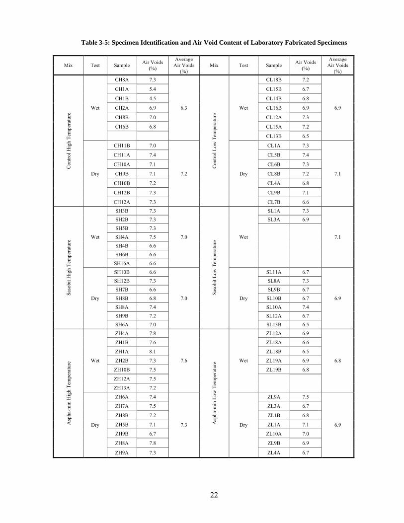
Table 3-5: Specimen Identification and Air Void Content of Laboratory Fabricated Specimens ................................................................................................................. 22
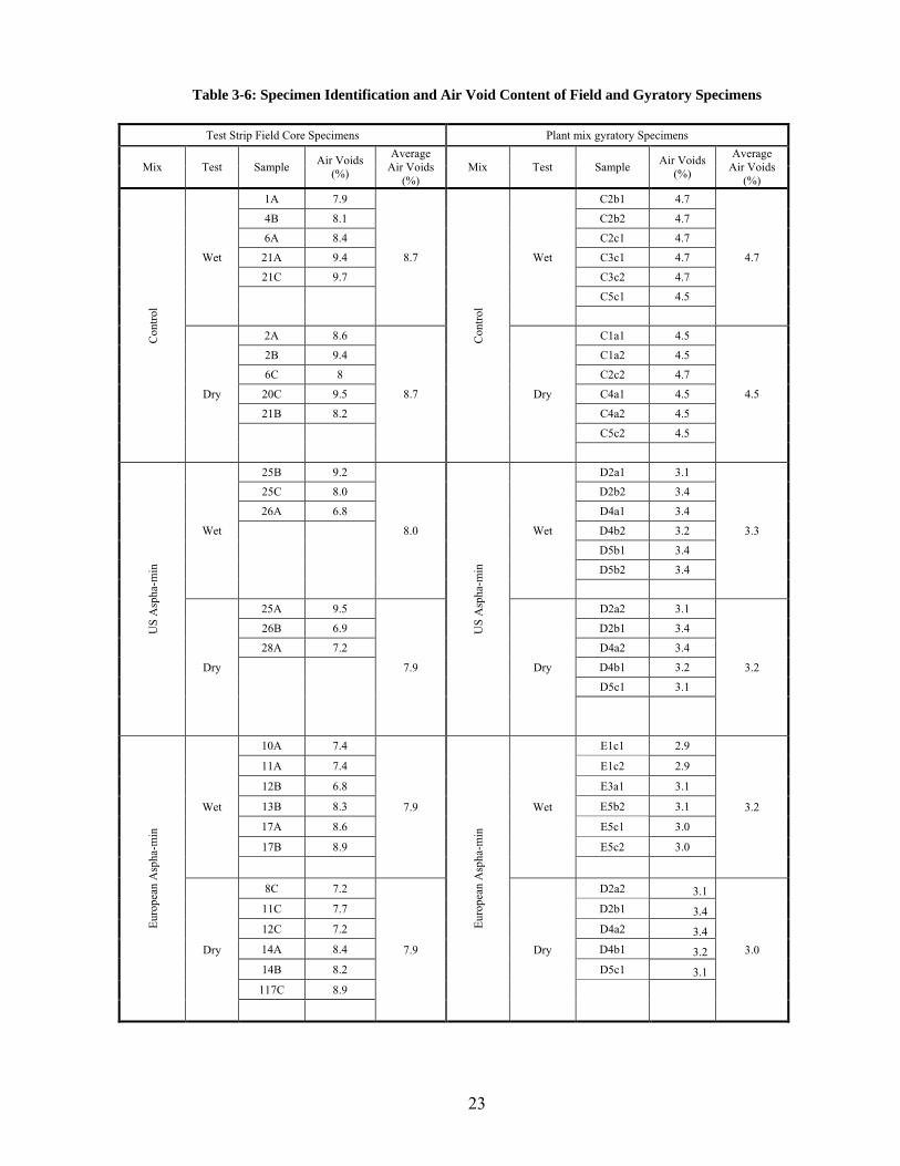
Table 3-6: Specimen Identification and Air Void Content of Field and Gyratory Specimens ................................................................................................................. 23
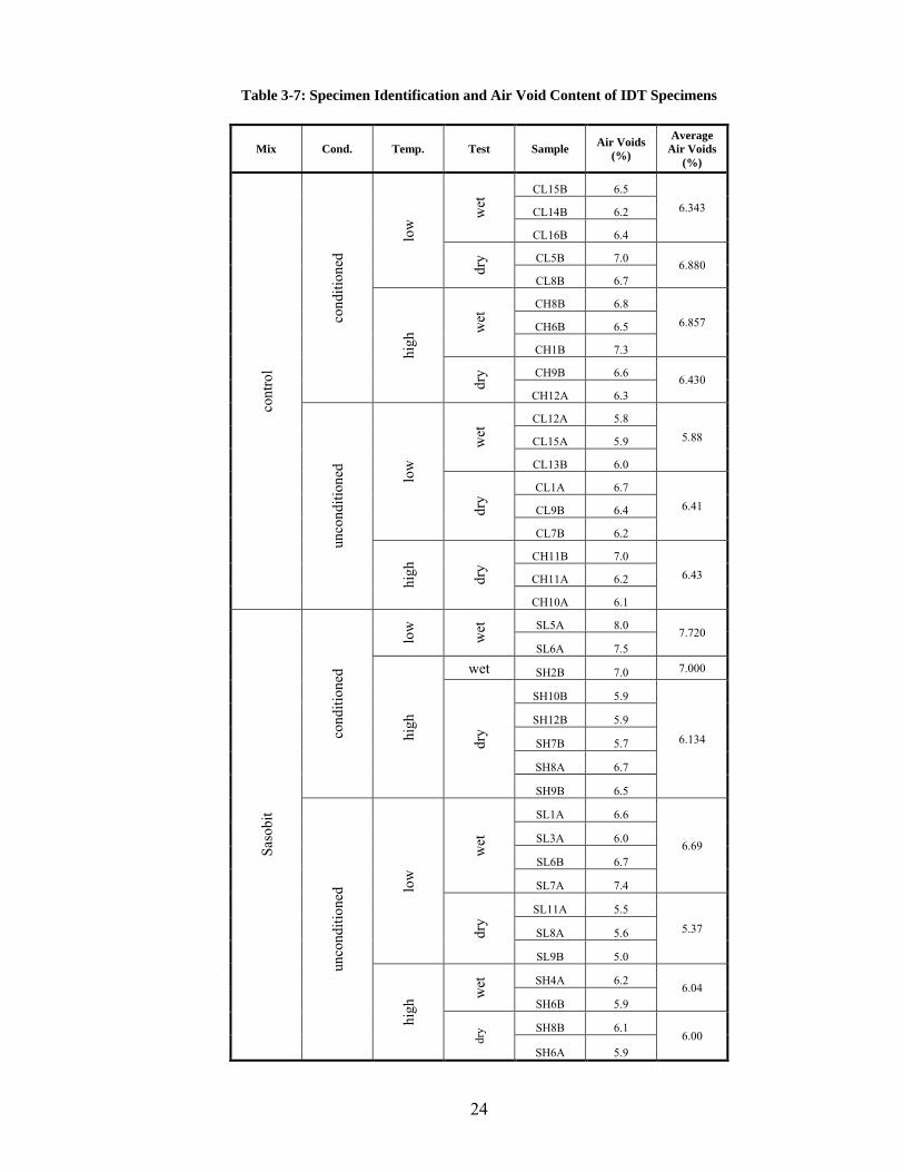
Table 3-7: Specimen Identification and Air Void Content of IDT Specimens ................. 24
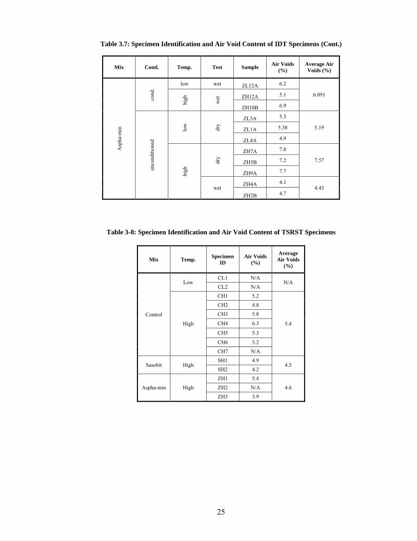
Table 3-8: Specimen Identification and Air Void Content of TSRST Specimens ........... 25 CHAPTER 5 Table 5-1: Comparison of Rut Depths for Plant Mix Gyratory Samples ......................... 45
Table 5-2: Comparison of Rut Depths of Laboratory Control Samples ........................... 46
Table 5-3: Comparison of Rut Depths of Sasobit Mixtures ............................................. 48
Table 5-4: Comparison of Rut Depths of Aspha-Min Vs. Laboratory Control Samples . 50
Table 5-5: Differences in rut depths among laboratory samples ...................................... 54
Table 5-6: Tensile strength summary ............................................................................... 56
Table 5-7: Comparison of IDT Strength Depths of US Aspha-Min and Sasobit Vs. Laboratory Control Samples ..................................................................................... 56
Table 5-8: m-values Obtained from the Master Curves of each Mixture ......................... 63
Table 5-9: Summary of TSRST Results ........................................................................... 65 APPENDICES Table B-0-1: Compaction data for trial asphalt binder content specimens ....................... 86
Table B-0-2: Volumetric properties of trial asphalt binder content specimens ................ 88 Table C-0-1: Field core cumulative rut depth summary ................................................... 93 Table D-0-1: Gyratory Specimen Cumulative Rut Depth Summary ................................ 98 Table E-0-1: Laboratory Fabricated Specimen Cumulative Rut Depth Summary ......... 105
vi
LIST OF FIGURES
FIGURE PAGE CHAPTER 3 Figure 3-1: 0.45 Power Gradation Chart for Elliot Aggregate Stockpiles .......................... 8
Figure 3-2: Sasobit Additive ............................................................................................... 9
Figure 3-3: Aspha-min Zeolite Additive ........................................................................... 10
Figure 3-4: Servopac Superpave Gyratory compactor and PC ......................................... 11
Figure 3-5: Corelok System Used to Determine Theoretical and Bulk Specific Gravities................................................................................................................................... 12
Figure 3-6: 0.45 Power chart for aggregate blend ............................................................ 13
Figure 3-7: Metal template Used to Prepare MMLS3 Specimens and a Cut and Prepared Specimen ................................................................................................................... 14
Figure 3-8: Third-Scale Model Mobile Load Simulator ................................................... 15
Figure 3-9: Schematic of MMLS3 Test Bed (13) ............................................................. 15
Figure 3-10: Specimens Clamped into MMLS3 Test Bed ................................................ 16
Figure 3-11: Wet heater Connected to MMLS3 Test Bed ................................................ 16
Figure 3-12: MMLS3 Dry Heating/Cooling Unit with Attached Heating Ducts ............. 17
Figure 3-13: Environmental Chamber with Attached Blowers ........................................ 18
Figure 3-14: MMLS3 Profilometer Resting on Index Bars .............................................. 19 CHAPTER 4 Figure 4-1: Individual Specimen and Average Rut Depth Versus Loading Interval ........ 30
Figure 4-2: IDT Load Fixture inside the Temperature Chamber ...................................... 32
Figure 4-3: D(t) Master Curve for Sasobit High Temperature Mixture ........................... 34
Figure 4-4: Schematic View of the TSRST Setup ............................................................ 35
Figure 4-5: Typical Stress Versus Temperature Curve ..................................................... 36
Figure 4-6: Schematic View of the Experimental Plan for Test Strip Field Core and Plant Mix Gyratory Specimens .......................................................................................... 37
Figure 4-7: Schematic View of the Experimental Plan For Test Strip Field Core and Plant Mix Gyratory Specimens .......................................................................................... 38
CHAPTER 5 Figure 5-1: Field Core Cumulative Rutting Summary ..................................................... 39
Figure 5-2: Field Core Cumulative Rutting up to 2000 Cycles ........................................ 40
Figure 5-3: Control Field Test Wet Cumulative Rutting Summary ................................. 41
Figure 5-4: Control field test dry cumulative rutting summary ........................................ 42
Figure 5-5: U.S. Aspha-min field test wet cumulative rutting summary .......................... 42
Figure 5-6: U.S. Aspha-min Field Test Dry Cumulative Rutting Summary .................... 43
Figure 5-7: Plant Mix Gyratory Cumulative Rutting Summary ....................................... 44
Figure 5-8: Wet/Dry Ratio of Plant Mix Gyratory Samples ............................................. 45
Figure 5-9: Laboratory Control Cumulative Rutting Summary ....................................... 46
Figure 5-10: Wet/Dry Ratio of Laboratory Control Samples at 100k loading ................. 47
Figure 5-11: Laboratory Sasobit Cumulative Rutting Summary ...................................... 48
vii
Figure 5-12: Wet/Dry rut Depth Ratio of Laboratory Sasobit Specimens at 100k Loading................................................................................................................................... 49
Figure 5-13: Laboratory Aspha-min Cumulative Rutting Summary ................................ 50
Figure 5-14: Wet/Dry Rut Depth Ratio of Laboratory Aspha-Min Samples at 100k Loading ..................................................................................................................... 51
Figure 5-15: Cumulative Rutting Summary for All Laboratory Specimens Fabricated at High Temperature ..................................................................................................... 52
Figure 5-16: Cumulative Rutting Summary for All Laboratory Specimens Fabricated at Low Temperature ...................................................................................................... 52
Figure 5-17: Cumulative Rutting Summary for All Laboratory Samples Tested Wet ..... 53
Figure 5-18: Cumulative Rutting Summary for All Laboratory Samples Tested Wet ..... 53
Figure 5-19: Wet/Dry Rut Ratio for All Mmls3 Tested Specimens at 100k Loading ...... 55
Figure 5-20: Laboratory Samples Dry Unconditioned Tensile Strength .......................... 57
Figure 5-21: Laboratory Samples Wet Unconditioned Tensile Strength .......................... 57
Figure 5-22: Plant Mix Gyratory Samples Tensile Strength ............................................ 58
Figure 5-23: Tensile Strength Ratio .................................................................................. 58
Figure 5-24: D(t) Curves for Sasobit High Temperature Mixture .................................... 59
Figure 5-25: D(t) Master Curve for Sasobit High Temperature Mixture ......................... 60
Figure 5-26: D(t) Master Curves for High Temperature Mixtures ................................... 61
Figure 5-27: D(t) Master Curves for Low Temperature Mixtures .................................... 61
Figure 5-28: D(t) Master Curves for Sasobit Mixture ...................................................... 62
Figure 5-29: Master curves for Aspha-min mixture ......................................................... 63
Figure 5-30: TSRST Fracture and Transition Stresses ..................................................... 66
Figure 5-31: TSRST Fracture and Transition Temperatures ............................................ 66
Figure 5-32: Average Slope of Each Group of Specimens ............................................... 67
Figure 5-33: Fracture Temperature Versus Fracture Stress .............................................. 68
Figure 5-34: Rank of Results For Rut Performance of the Test Strip Mixes ................... 70
Figure 5-35: Ranking of Results for Rut Performance of the Lab Fabricated Specimens 71
Figure 5-36: Ranking of Results for Moisture Susceptibility Performance of the Lab Fabricated Specimens Using TSR ............................................................................ 72
Figure 5-37: Rank of Results for Thermal Cracking Performance of the Lab Fabricated Specimens ................................................................................................................. 73
Figure 5-38: Ranking of Results for Moisture Susceptibility using MMLS3 Wet/Dry Ratio .......................................................................................................................... 74
Figure 5-39: Rank of Results for Moisture Susceptibility of the Lab. Fabricated Specimens .................................................................. Error! Bookmark not defined.
APPENDICES Figure B-0-1: Densification curves for trial asphalt binder content specimens ................ 86
Figure B-0-2: Mixture design volumetric properties plots ............................................... 87
Figure C-0-1: European aspha-min wet test ..................................................................... 90
Figure C-0-2: European aspha-min dry test ...................................................................... 90
Figure C-0-3: US Aspha-min wet test .............................................................................. 91
Figure C-0-4: US Aspha-min dry test ............................................................................... 91
Figure C-0-5: Control mix wet test ................................................................................... 92
viii
Figure C-0-6: Control Mix Dry Test ................................................................................. 92
Figure D-0-1: European Aspha-min Wet Test .................................................................. 95
Figure D-0-2: European Aspha-min Dry Test .................................................................. 95
Figure D-0-3: US Aspha-min Wet Test ............................................................................ 96
Figure D-0-4: US Aspha-min Dry Test ............................................................................ 96
Figure D-0-5: Control Mix Wet Test ................................................................................ 97
Figure D-0-6: Control Mix Dry Test ................................................................................ 97
Figure E-0-1: Control Mix Hot Mix Temp Wet Test ..................................................... 100
Figure E-0-2: Control Mix Hot Mix Temp Dry Test ...................................................... 100
Figure E-0-3: Control Mix Warm Mix Temp Wet Test ................................................. 101
Figure E-0-4: Control Mix Warm Mix Temp Dry Test .................................................. 101
Figure E-0-5: Sasobit Mix Hot Mix Temp Wet Test ...................................................... 102
Figure E-0-6: Sasobit Mix Hot Mix Temp Dry Test ...................................................... 102
Figure E-0-7: Sasobit Mix Warm Mix Temp Wet Test .................................................. 103
Figure E-0-8: Sasobit Mix Warm Mix Temp Dry Test .................................................. 103
Figure E-0-9: Aspha-min Mix Hot Mix Temp Wet Test ................................................ 104
Executive Summary This paper describes the results of a laboratory study conducted to evaluate the influence of Aspha-min® and Sasobit® additives on the behaviour of warm asphalt mixtures. Specimens were compacted at two temperatures, 100 and 1458C, and were subjected to two different testing procedures. The one-third model mobile traffic simulator and the thermal stress restrained specimen test were chosen to assess the susceptibility to moisture and thermal cracking. Results showed that warm asphalt mixtures prepared with Sasobit may be more susceptible to moisture damage, and both additives may negatively impact the low-temperature cracking performance compared with the control mixture.

1
CHAPTER 1
INTRODUCTION
1.1 - BACKGROUND OF RESEARCH
Warm mix asphalt (WMA) technologies were first pursued in Europe as a means of reducing the emission of greenhouse gasses during asphalt production. Warm mix technologies allow for mixing and compaction temperatures to be reduced 2 to 38°C below that of typical hot mix asphalt (HMA). Popularity of WMA is rising in the United States due to the reduction in emissions, decreased energy cost to the production plants, and less aging of the asphalt binder. There are several other potential benefits to WMA including the ability to extend the paving season into cooler weather, allow longer hauling distances, and use as a compaction aid for stiffer asphalt mixtures. The production of warm mix asphalt typically involves introducing an additive to the heated aggregate and liquid asphalt binder mixture. There are several warm mix additives that work by creating a reduction in viscosity of the asphalt binder. Reduced viscosity allows better coating of the aggregate structure and reduces the temperature required to achieve adequate workability of the mixture. Although there are many possible advantages to warm mix asphalt, the potential negative impacts on the performance of the mixtures must be fully evaluated. Laboratory testing of warm mix asphalt has shown the possibility of increased moisture sensitivity in comparison to typical hot mix asphalt. Moisture damage reduces the strength and performance capabilities of asphalt pavements. Before warm mix asphalt technologies are implemented in large scale paving projects, the performance and quality of the mixtures must be evaluated. The New Hampshire Department of Transportation (NHDOT) provided funding for this research. The results of this research will help the NHDOT evaluate the performance of WMA pavements in the lab under accelerated loading conditions that are representative of actual field conditions. This research will provide information that the DOT can use to make decisions on the use of WMA pavements in New Hampshire.
1.2 - OBJECTIVE OF RESEARCH
The objective of this research was to evaluate the moisture and low temperature cracking susceptibility of warm mixes made using Aspha-min and Sasobit additives. Evaluation of moisture susceptibility was accomplished by testing lab specimens, available cores, and field sections using the accelerated loading in the lab. Low temperature cracking performance was evaluated by testing lab specimens according to AASHTO T322 Standard Method of Test for Determining the Creep Compliance and
Strength of Hot-Mix Asphalt (HMA) Using the Indirect Tensile Test Device, and

2
AASHTO Standard Test Method for Thermal Stress Restrained Specimen Tensile
Strength
1.3 - REPORT ORGANIZATION Chapter 2 of this report presents an introduction to warm mix asphalt and moisture induced damage as well as the current state of research on WMA. Chapter 3 discusses the materials and mix designs used in this research, specimen fabrication, laboratory set-up, and testing equipment used. The test method and data analysis used to interpret the testing results are presented in Chapter 4. The results obtained and a discussion of these results is provided in Chapter 5. Chapter 6 includes conclusions and recommendations for future research on warm mix asphalt.
3
CHAPTER 2
LITERATURE REVIEW
2.1 - WARM MIX ASPHALT
Warm mix asphalt (WMA) technologies allow for the production and placement of asphalt as temperatures 20 to 55°C lower than typical hot mix asphalt (HMA) (1). These technologies, typically in the form of additives, reduce the viscosity of the asphalt binder, allowing it to fully coat the aggregate mix at lower temperatures.
Development of WMA technologies as a means of reducing greenhouse gas emissions began in Europe as a result of the German Bitumen Forum in 1997 (2). The Kyoto Protocol of 1997 was adopted to commit the European community to reduce greenhouse gas emissions an average of 5% against 1990 levels by the year 2012 (1). The utilization of WMA was the European response to the Kyoto Protocol and a means of ensuring sustainable development for the future.
Although the United States has not ratified the Kyoto Protocol, WMA research has begun as a result of other legislation. The US Environmental Protection Agency issued the Clean Air Interstate Rule (CAIR) in 2005, which was designed to reduce sulfur dioxide and nitrogen oxide emissions, both of which contribute to the formation of ground-level ozone. A reduction in ground-level ozone production from asphalt plants may be achieved through use of WMA. (1)
Several benefits are possible with WMA in addition to lower greenhouse gas emissions. A reduction in odor and fumes that may contribute to health issues are possible and have been proven (3). Lower production temperatures at asphalt mixing plants require less fuel to heat the asphalt binder. Based on a 28°C (50°F) reduction in temperature, fuel consumption is reduced by an average of 11% (1). Hauling loads of asphalt over longer distances as well as extending the paving season into cool weather without critical temperature loss may be possible utilizing WMA technologies.
Currently, there are about twenty additives or processes to make WMA. This research project focused on two: Aspha-min® and Sasobit®. (referred to as Aspha-min and Sasobit hereafter)
Aspha-min is a zeolite asphalt modifier and consists of a manufactured synthetic sodium aluminum silicate that has been hydro-thermally crystallized. Aspha-min is a product of Eurovia Services GmbH based in Bottrop, Germany. It is a framework silicate that has large empty spaces in its crystal structure. These empty spaces hold water, which is released in the presence of heat. Aspha-min contains 21% water by mass that is released in the temperature range of 85 to 182˚C (185 to 360˚F). Eurovia recommends
that Aspha-min be added to the heated aggregate at the same time as the liquid binder at a rate of 0.3% by mass of the mix. When added to the aggregate-liquid binder mix, Aspha-
4
min releases its internal moisture which microscopically foams the liquid binder, allowing it to better coat the aggregate. (5)
Sasobit, a product of Sasol Wax, is a fine crystalline, long-chain aliphatic polymethylene hydrocarbon produced from coal gassification using the Fischer-Tropsch process. The long molecular chains of Sasobit give the wax a higher melting point than typical paraffin waxes, and the smaller crystalline structure of Sasobit reduces its brittleness at low temperatures when compared to paraffin waxes. Sasobit has a congealing temperature of approximately 102˚C (216˚F) and is completely soluble in
liquid asphalt binder above 120˚C (248˚F). Sasol Wax recommends that Sasobit be added
to the liquid asphalt binder at 0.8 to 3.0% by mass of the binder. When added to the liquid binder, Sasobit reduces the viscosity of the asphalt binder, allowing it to coat the aggregate at temperatures up to 54˚C (97˚F) lower than HMA mixing temperatures. (6)
2.2 - MOISTURE DAMAGE
Moisture susceptibility is the deterioration of asphalt pavements due to the damaging influences of moisture. Moisture-induced damage, or stripping, depends on many variables but will not occur in the absence of moisture. The strength of an asphalt pavement comes from the frictional resistance of the aggregate as well as the cohesional resistance of the asphalt binder and aggregate grain interlock. The cohesional resistance can weaken or deteriorate completely if the bond between the binder and the aggregate is poor. Failure at the binder-aggregate interface can lead to premature damage to the asphalt pavement. Stripping can be difficult to identify as its physical manifestation can be in the form of rutting, shoving, corrugations, raveling, or cracking. The best way to confirm stripping is to physically break open a core sample from the pavement structure and look for partially or fully uncoated aggregate in the cross-section. (7) Although physical properties of the asphalt binder and the aggregate can contribute to stripping, moisture susceptibility has a number of externally contributing factors as well. Inadequate pavement drainage permits saturation of the air voids within the pavement structure. An increase in ambient temperature can cause expansion of the moisture leading to excessive pore pressure and stripping. Additionally, traffic induced stress on saturated pores can lead to binder-aggregate bond failure. (8) Proper mix density is essential in combating moisture-induced damage. A properly designed mixture can be subject to stripping if the air void content is high enough to allow moisture into the structure. Pavements compacted to 4 to 5% air voids are almost impervious due to the lack of interconnected void space. Pavement air voids content are typically between 6 to 8% but the mixture will continue to densify to 3 to 5% air voids under normal trafficking. When pavements are compacted with more than 8% air voids they remain pervious to moisture for an extended period of time. The high air void content of these pavements allows moisture to build, introducing the possibility of moisture-induced damage. (7, 8)
Inadequate drying of aggregate before and during the mixing process has been shown to contribute to moisture susceptibility of asphalt mixtures. Dry aggregates will bond more effectively with asphalt binder than moist aggregates. (7)
5
The moisture susceptibility of warm mix asphalt is in question. Because the mixing process for WMA occurs at a low temperature, the aggregate may not be completely dry prior to mixing, causing a weaker bond between the aggregate and asphalt binder. Additionally, some additives used during production of WMA release moisture to the mixture in order to lower the viscosity of the aggregate binder. This added moisture may contribute to moisture susceptibility, regardless of how thoroughly the aggregate was dried prior to mixing. Any moisture present in the mix may prohibit a complete bond between the aggregate surface and the asphalt binder and contribute to moisture damage.
The property of asphalt most commonly linked with stripping is viscosity (7). The lowering of the asphalt binder viscosity through the use of WMA additives may contribute to the moisture susceptibility of warm asphalt mixtures. High viscosity asphalt binders have shown to be more resistant to displacement by water than low viscosity asphalt binders.
2.3 - CURRENT STATE OF RESEARCH Research on warm mix asphalt technologies has only begun in the United States
in recent years. In 2006, the Warm Mix Asphalt Technical Working Group (WMA TWG) was initiated by the National Asphalt Pavement Association (NAPA) and the Federal Highway Administration (FHWA) to promote and implement proactive WMA policies, practices, and procedures and to evaluate and implement WMA technologies. The TWG is made up of representatives from FHWA, NAPA, State Highway Agencies (SHA), State Asphalt Pavement Associations (SAPA), American Association of State Highway Transportation Officials (AASHTO), National Center for Asphalt Technology (NCAT), the Hot Mix Asphalt Industry, Labor, and National Institute for Occupational Safety and Health (NIOSH). The WMA TWG meets several times a year and provides a forum-like environment where government and industry officials can share new and innovative or proven WMA concepts. (9) Initial research on the feasibility of using WMA technologies in the United States was conducted in 2005 through a cooperative agreement between NCAT and FHWA. Sasobit, Aspha-min, and WAM Foam were studied to determine any affect the additives have on compactability, resilient modulus, rutting potential, and moisture susceptibility (9). Results of the Sasobit and Aspha-min investigations are of interest to this research.
The Sasobit study indicated that compactability improved and Resilient Modulus was not affected in mixes made with Sasobit. Most notable to this research is the indication that Sasobit mixes tended to have increased rutting resistance at low mixing temperatures when compared with control mixes. Also, stripping and reduced tensile strength in both Sasobit and control mixes were evident, but the addition of an anti-stripping agent improved the tensile strength ratios to above Superpave criteria. (6)
Similar to the results of the Sasobit study, the Aspha-min study indicated that the addition of Aspha-min to the mixture improved compactability and had no affect on Resilient Modulus of the mixture. The study indicated that rutting potential was not affected by the addition of Aspha-min, but reduced tensile strength and stripping was apparent in both Aspha-min and control specimens mixed at low temperatures. The addition of hydrated lime improved the tensile strength ratios to above Superpave criteria.
6
The increased susceptibility to moisture damage was attributed to residual moisture left in the aggregate at the lower mixing and compaction temperatures. (5)
In order to gain firsthand experience with WMA technologies being used in Europe, AASHTO and FHWA organized a scanning tour to four European countries and invited 13 ‘materials experts’ to perform research on the tour. In May 2007,
representatives from AASHTO, FHWA, NAPA, Asphalt Institute (AI), asphalt suppliers, contractors, and consultants visited Norway, Germany, Belgium, and France to assess and evaluate various WMA technologies. The tour allowed the group to discuss current technologies with European agencies, view in-service WMA pavements, visit construction sites, and learn how HMA practices in Europe and the United States may affect WMA use. (10)
Observations and discussions during the scanning tour led the group to several conclusions regarding WMA implementation in the U.S.: WMA should be an acceptable alternative to HMA; an approval system based on WMA performance needed to be developed; best practice guidelines for aggregate handling and storage to minimize moisture content needed to be developed; more field trials in the U.S. were needed; and the economic factors such as additive costs, plant modifications, and emissions compliance needed to be identified and tracked. (10)
Currently, there are two research projects being conducted by the National Cooperative Highway Research Program (NCHRP), NCHRP 09-43: Mix Design
Practices for Warm Mix Asphalt, and NCHRP 09-47: Engineering Properties, Emissions,
and Field Performance of Warm Mix Asphalt Technologies. The objective of NCHRP 09-43, due to be complete in 2010, is to develop a mix design procedure for WMA based on the Superpave mix design procedure which will include performance tests to evaluate field performance. The objectives of NCHRP 09-47 are 1) to establish relationships among engineering properties of WMA binders and mixes and the field performance of WMA pavements, 2) to determine relative measures of performance between WMA and HMA pavements, 3) to compare production and laydown practices and costs between WMA and HMA pavements, and 4) to provide relative emissions measurement of WMA technologies as compared to HMA technologies. This project will include at least two full-scale field trials, complemented by accelerated pavement testing when possible. (9)
Although warm mix asphalt testing is relatively new in the United States, there is a progressive move to evaluate and understand the possibilities of WMA. Initial research indicates that there is increased susceptibility to moisture induced damaged that is possibly due to incomplete drying of the aggregate prior to mixing. The specimens for this research will be mixed with aggregate oven-dried for a minimum of 8 hours in order to eliminate the possibility of residual moisture. By utilizing only completely dry aggregate, the effect of warm mix additives on the moisture susceptibility of test specimens is isolated. Testing control specimens and specimens with warm mix additives in the presence of moisture in the Third-scale Model Mobile Load Simulator (MMLS3) will help identify if the additives contribute to moisture damage in the pavement specimens.
7
CHAPTER 3 MATERIALS AND METHODS
3.1 - MATERIALS
3.1.1 - Hooksett Crushed Stone Test Strip Specimens
In November 2005, a test strip was laid at the entrance to Hooksett Crushed Stone in Hooksett, NH. The test strip consisted of two control sections, two sections containing a European Aspha-min© zeolite, and one section containing a domestic Aspha-min zeolite. Each mix type for the test strip was produced with an asphalt content of 5.8%. The material for each section was mixed in the on-site batch plant and field compacted. Field cores were obtained from each section and brought to the lab for testing. These samples are referred to as “field cores” throughout the report. Prior to placement, loose material from each section was obtained and compacted in the on-site laboratory. These specimens will be referred to as “gyratory” specimens.
3.1.2 - Material Selection
Materials for the laboratory fabricated specimens were selected to be typical of the materials used by the New Hampshire Department of Transportation (NHDOT) in state paving projects. A single aggregate gradation was selected to be mixed with a single performance grade (PG) asphalt binder to minimize the number of variables in the mixtures. PIKE Industries in Portsmouth, NH was contacted for a typical NH state mix using a single 12.5 mm nominal maximum aggregate size aggregate blend. The blend obtained from PIKE Industries utilized Elliot crushed aggregate and was used as a guideline for the gradation in this research. The warm mix additives Sasobit and Aspha-min were chosen for their ease of use in laboratory mixing and for their use in previous research done to evaluate warm asphalt mixtures and also based on the interest of NHDOT.
3.1.3 - Aggregate
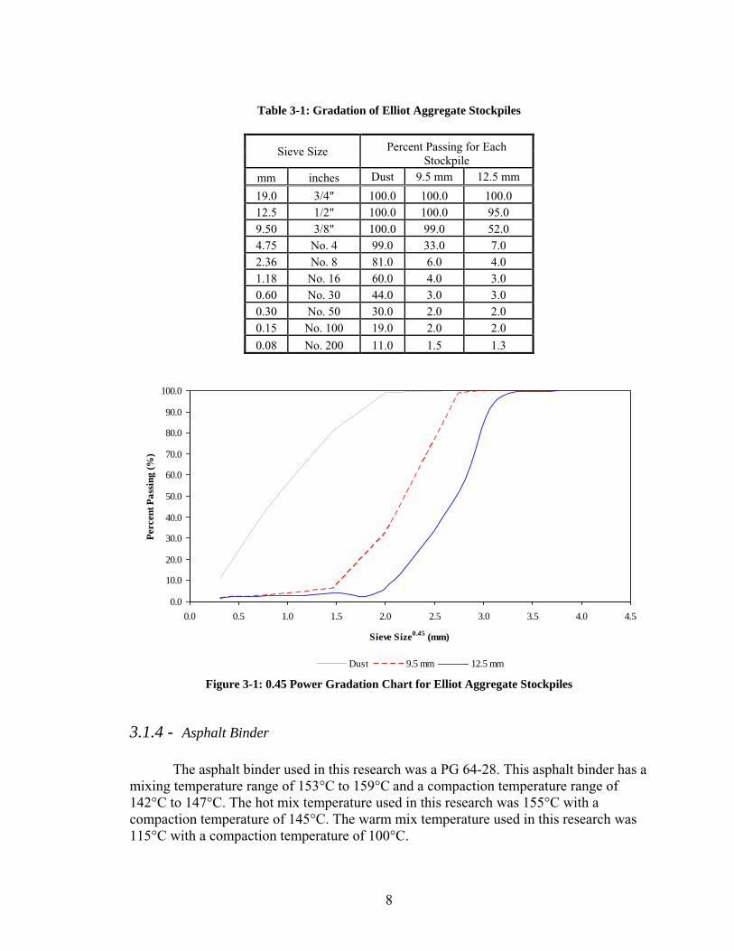
The aggregate for this research was obtained from PIKE Industries in Portsmouth, NH. The Elliot aggregate used in this research came from the Dust, 9.5 mm, and 12.5 mm stockpiles. The gradation of the aggregate is given in Table 3-1 and is illustrated in Figure 3-1. The required aggregate from each stockpile was loaded into separate 50 gallon barrels and transported to the University of New Hampshire. The stockpiles were stored in separate barrels to minimize the sieving required to obtain a specific size aggregate for sample preparation.
8
Table 3-1: Gradation of Elliot Aggregate Stockpiles
Sieve Size Percent Passing for Each Stockpile
mm inches Dust 9.5 mm 12.5 mm
19.0 3/4" 100.0 100.0 100.0 12.5 1/2" 100.0 100.0 95.0 9.50 3/8" 100.0 99.0 52.0 4.75 No. 4 99.0 33.0 7.0 2.36 No. 8 81.0 6.0 4.0 1.18 No. 16 60.0 4.0 3.0 0.60 No. 30 44.0 3.0 3.0 0.30 No. 50 30.0 2.0 2.0 0.15 No. 100 19.0 2.0 2.0
0.08 No. 200 11.0 1.5 1.3
Figure 3-1: 0.45 Power Gradation Chart for Elliot Aggregate Stockpiles
3.1.4 - Asphalt Binder
The asphalt binder used in this research was a PG 64-28. This asphalt binder has a mixing temperature range of 153°C to 159°C and a compaction temperature range of 142°C to 147°C. The hot mix temperature used in this research was 155°C with a compaction temperature of 145°C. The warm mix temperature used in this research was 115°C with a compaction temperature of 100°C.
0.0
10.0
20.0
30.0
40.0
50.0
60.0
70.0
80.0
90.0
100.0
0.0 0.5 1.0 1.5 2.0 2.5 3.0 3.5 4.0 4.5
Sieve Size0.45
(mm)
Percen
t P
ass
ing
(%
)
Dust 9.5 mm 12.5 mm
9
3.1.5 - Sasobit
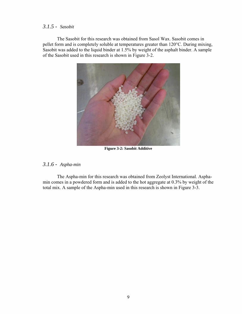
The Sasobit for this research was obtained from Sasol Wax. Sasobit comes in pellet form and is completely soluble at temperatures greater than 120°C. During mixing, Sasobit was added to the liquid binder at 1.5% by weight of the asphalt binder. A sample of the Sasobit used in this research is shown in Figure 3-2.
Figure 3-2: Sasobit Additive
3.1.6 - Aspha-min
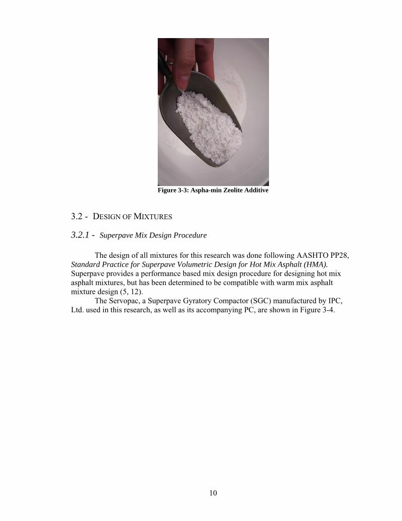
The Aspha-min for this research was obtained from Zeolyst International. Aspha-min comes in a powdered form and is added to the hot aggregate at 0.3% by weight of the total mix. A sample of the Aspha-min used in this research is shown in Figure 3-3.
10
Figure 3-3: Aspha-min Zeolite Additive
3.2 - DESIGN OF MIXTURES
3.2.1 - Superpave Mix Design Procedure
The design of all mixtures for this research was done following AASHTO PP28, Standard Practice for Superpave Volumetric Design for Hot Mix Asphalt (HMA).
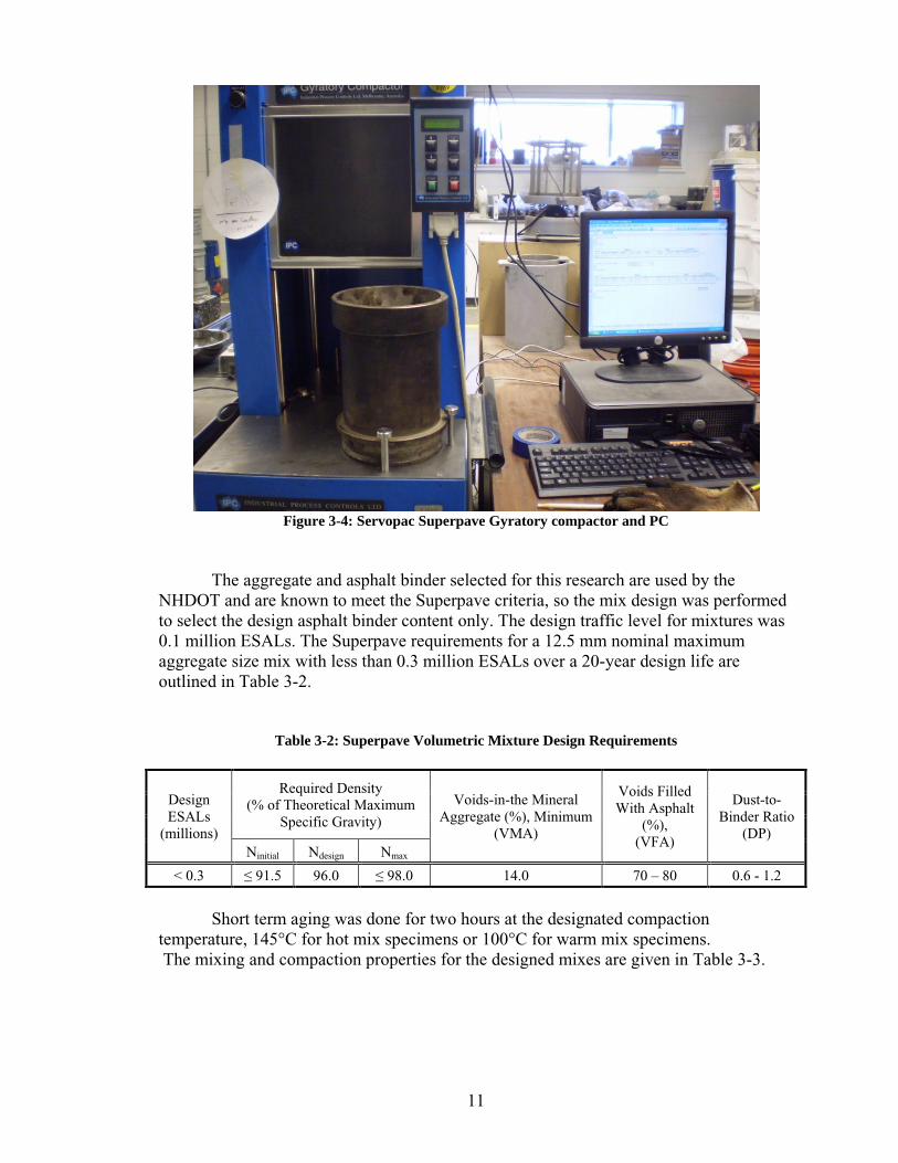
Superpave provides a performance based mix design procedure for designing hot mix asphalt mixtures, but has been determined to be compatible with warm mix asphalt mixture design (5, 12). The Servopac, a Superpave Gyratory Compactor (SGC) manufactured by IPC, Ltd. used in this research, as well as its accompanying PC, are shown in Figure 3-4.
11
Figure 3-4: Servopac Superpave Gyratory compactor and PC
The aggregate and asphalt binder selected for this research are used by the NHDOT and are known to meet the Superpave criteria, so the mix design was performed to select the design asphalt binder content only. The design traffic level for mixtures was 0.1 million ESALs. The Superpave requirements for a 12.5 mm nominal maximum aggregate size mix with less than 0.3 million ESALs over a 20-year design life are outlined in Table 3-2.
Table 3-2: Superpave Volumetric Mixture Design Requirements
Design ESALs
(millions)
Required Density (% of Theoretical Maximum
Specific Gravity)
Voids-in-the Mineral Aggregate (%), Minimum
(VMA)
Voids Filled With Asphalt
(%), (VFA)
Dust-to-Binder Ratio
(DP) Ninitial Ndesign Nmax
< 0.3 ≤ 91.5 96.0 ≤ 98.0 14.0 70 – 80 0.6 - 1.2
Short term aging was done for two hours at the designated compaction temperature, 145°C for hot mix specimens or 100°C for warm mix specimens. The mixing and compaction properties for the designed mixes are given in Table 3-3.
12
Table 3-3: Summary of Mixing and Compaction Parameters
Parameter Value
Hot Mix Warm Mix
Asphalt Binder Grade PG 64-28 Initial Aggregate Drying Time and Temperature 8 Hrs @ 170°C 8 Hrs @ 130°C
Mixing Temperature 155°C 115°C Compaction Temperature 145°C 100°C
Short Term Aging Time and Temperature 2 Hrs @ 145°C 2 Hrs @ 100°C Design Number of Gyrations, Ndes 50 50
Compaction Ram Pressure 600 kPa Compaction Mold Diameter 150 mm
Compaction Rate 30 gyrations/minute Compaction Angle 1.25°
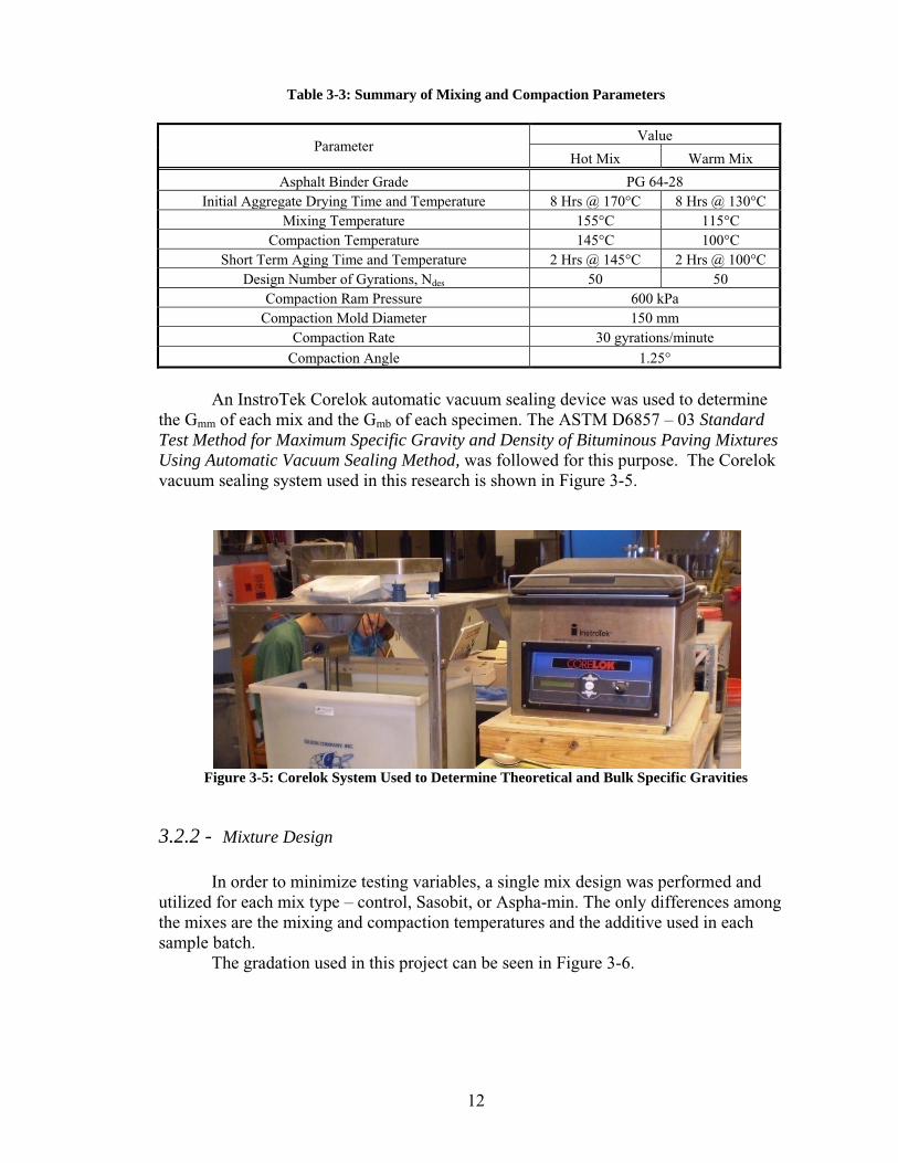
An InstroTek Corelok automatic vacuum sealing device was used to determine the Gmm of each mix and the Gmb of each specimen. The ASTM D6857 – 03 Standard
Test Method for Maximum Specific Gravity and Density of Bituminous Paving Mixtures
Using Automatic Vacuum Sealing Method, was followed for this purpose. The Corelok
vacuum sealing system used in this research is shown in Figure 3-5.
Figure 3-5: Corelok System Used to Determine Theoretical and Bulk Specific Gravities
3.2.2 - Mixture Design
In order to minimize testing variables, a single mix design was performed and utilized for each mix type – control, Sasobit, or Aspha-min. The only differences among the mixes are the mixing and compaction temperatures and the additive used in each sample batch. The gradation used in this project can be seen in Figure 3-6.
13
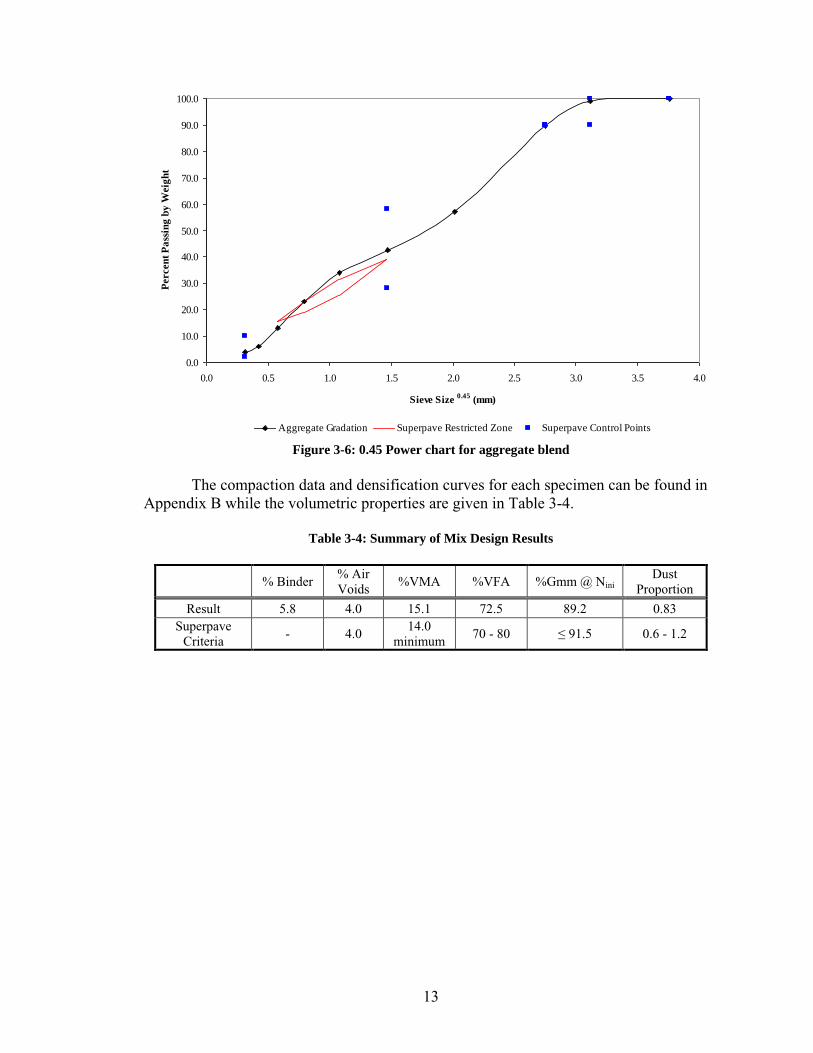
Figure 3-6: 0.45 Power chart for aggregate blend
The compaction data and densification curves for each specimen can be found in
Appendix B while the volumetric properties are given in Table 3-4.
Table 3-4: Summary of Mix Design Results
% Binder % Air Voids
%VMA %VFA %Gmm @ Nini Dust
Proportion
Result 5.8 4.0 15.1 72.5 89.2 0.83 Superpave
Criteria - 4.0
14.0 minimum
70 - 80 ≤ 91.5 0.6 - 1.2
0.0
10.0
20.0
30.0
40.0
50.0
60.0
70.0
80.0
90.0
100.0
0.0 0.5 1.0 1.5 2.0 2.5 3.0 3.5 4.0
Sieve Size 0.45
(mm)
Percen
t P
ass
ing
by
Weig
ht
Aggregate Gradation Superpave Restricted Zone Superpave Control Points
14
3.3 - LABORATORY SETUP AND TESTING EQUIPMENT
3.3.1 - Wet Saw Jig and Template
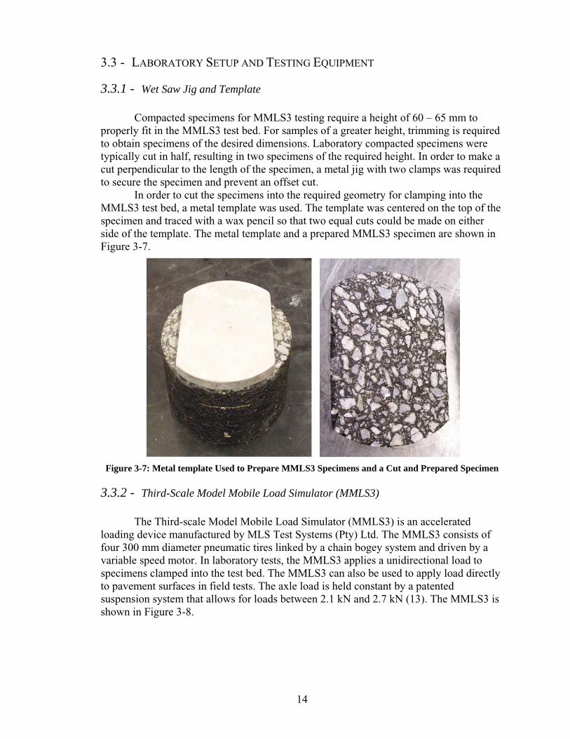
Compacted specimens for MMLS3 testing require a height of 60 – 65 mm to properly fit in the MMLS3 test bed. For samples of a greater height, trimming is required to obtain specimens of the desired dimensions. Laboratory compacted specimens were typically cut in half, resulting in two specimens of the required height. In order to make a cut perpendicular to the length of the specimen, a metal jig with two clamps was required to secure the specimen and prevent an offset cut. In order to cut the specimens into the required geometry for clamping into the MMLS3 test bed, a metal template was used. The template was centered on the top of the specimen and traced with a wax pencil so that two equal cuts could be made on either side of the template. The metal template and a prepared MMLS3 specimen are shown in Figure 3-7.
Figure 3-7: Metal template Used to Prepare MMLS3 Specimens and a Cut and Prepared Specimen
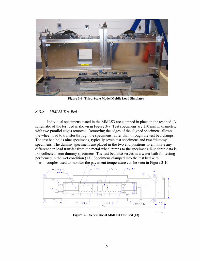
3.3.2 - Third-Scale Model Mobile Load Simulator (MMLS3)
The Third-scale Model Mobile Load Simulator (MMLS3) is an accelerated loading device manufactured by MLS Test Systems (Pty) Ltd. The MMLS3 consists of four 300 mm diameter pneumatic tires linked by a chain bogey system and driven by a variable speed motor. In laboratory tests, the MMLS3 applies a unidirectional load to specimens clamped into the test bed. The MMLS3 can also be used to apply load directly to pavement surfaces in field tests. The axle load is held constant by a patented suspension system that allows for loads between 2.1 kN and 2.7 kN (13). The MMLS3 is shown in Figure 3-8.
15
Figure 3-8: Third-Scale Model Mobile Load Simulator
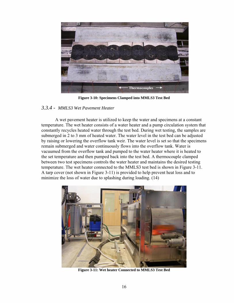
3.3.3 - MMLS3 Test Bed
Individual specimens tested in the MMLS3 are clamped in place in the test bed. A schematic of the test bed is shown in Figure 3-9. Test specimens are 150 mm in diameter, with two parallel edges removed. Removing the edges of the aligned specimens allows the wheel load to transfer through the specimens rather than through the test bed clamps. The test bed holds nine specimens, typically seven test specimens and two “dummy”
specimens. The dummy specimens are placed in the two end positions to eliminate any difference in load transfer from the metal wheel ramps to the specimens. Rut depth data is not collected from dummy specimens. The test bed also serves as a water bath for testing performed in the wet condition (13). Specimens clamped into the test bed with thermocouples used to monitor the pavement temperature can be seen in Figure 3-10.
Figure 3-9: Schematic of MMLS3 Test Bed (13)
16
Figure 3-10: Specimens Clamped into MMLS3 Test Bed
3.3.4 - MMLS3 Wet Pavement Heater
A wet pavement heater is utilized to keep the water and specimens at a constant temperature. The wet heater consists of a water heater and a pump circulation system that constantly recycles heated water through the test bed. During wet testing, the samples are submerged in 2 to 3 mm of heated water. The water level in the test bed can be adjusted by raising or lowering the overflow tank weir. The water level is set so that the specimens remain submerged and water continuously flows into the overflow tank. Water is vacuumed from the overflow tank and pumped to the water heater where it is heated to the set temperature and then pumped back into the test bed. A thermocouple clamped between two test specimens controls the water heater and maintains the desired testing temperature. The wet heater connected to the MMLS3 test bed is shown in Figure 3-11. A tarp cover (not shown in Figure 3-11) is provided to help prevent heat loss and to minimize the loss of water due to splashing during loading. (14)
Figure 3-11: Wet heater Connected to MMLS3 Test Bed
17
3.3.5 - MMLS3 Dry Heating/Cooling Unit
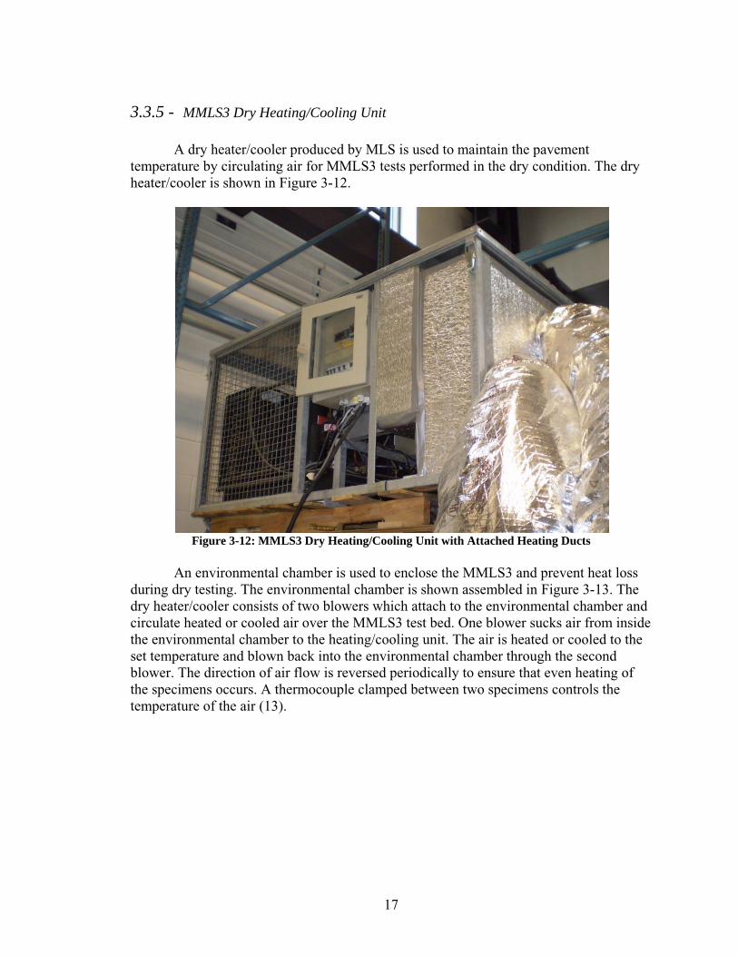
A dry heater/cooler produced by MLS is used to maintain the pavement temperature by circulating air for MMLS3 tests performed in the dry condition. The dry heater/cooler is shown in Figure 3-12.
Figure 3-12: MMLS3 Dry Heating/Cooling Unit with Attached Heating Ducts
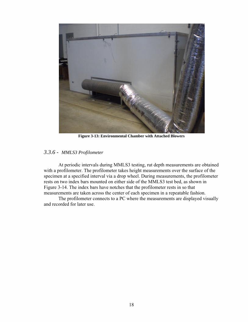
An environmental chamber is used to enclose the MMLS3 and prevent heat loss during dry testing. The environmental chamber is shown assembled in Figure 3-13. The dry heater/cooler consists of two blowers which attach to the environmental chamber and circulate heated or cooled air over the MMLS3 test bed. One blower sucks air from inside the environmental chamber to the heating/cooling unit. The air is heated or cooled to the set temperature and blown back into the environmental chamber through the second blower. The direction of air flow is reversed periodically to ensure that even heating of the specimens occurs. A thermocouple clamped between two specimens controls the temperature of the air (13).
18
Figure 3-13: Environmental Chamber with Attached Blowers
3.3.6 - MMLS3 Profilometer
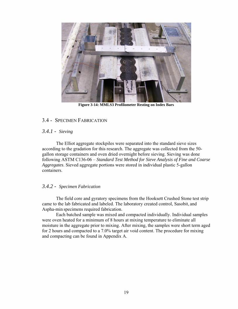
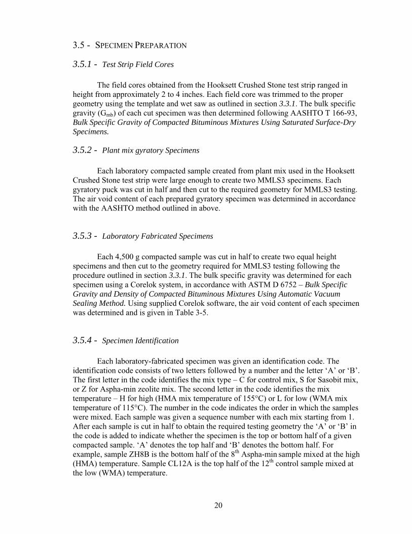
At periodic intervals during MMLS3 testing, rut depth measurements are obtained with a profilometer. The profilometer takes height measurements over the surface of the specimen at a specified interval via a drop wheel. During measurements, the profilometer rests on two index bars mounted on either side of the MMLS3 test bed, as shown in Figure 3-14. The index bars have notches that the profilometer rests in so that measurements are taken across the center of each specimen in a repeatable fashion. The profilometer connects to a PC where the measurements are displayed visually and recorded for later use.
19
Figure 3-14: MMLS3 Profilometer Resting on Index Bars
3.4 - SPECIMEN FABRICATION
3.4.1 - Sieving
The Elliot aggregate stockpiles were separated into the standard sieve sizes according to the gradation for this research. The aggregate was collected from the 50-gallon storage containers and oven dried overnight before sieving. Sieving was done following ASTM C136-06 – Standard Test Method for Sieve Analysis of Fine and Coarse
Aggregates. Sieved aggregate portions were stored in individual plastic 5-gallon containers.
3.4.2 - Specimen Fabrication
The field core and gyratory specimens from the Hooksett Crushed Stone test strip came to the lab fabricated and labeled. The laboratory created control, Sasobit, and Aspha-min specimens required fabrication. Each batched sample was mixed and compacted individually. Individual samples were oven heated for a minimum of 8 hours at mixing temperature to eliminate all moisture in the aggregate prior to mixing. After mixing, the samples were short term aged for 2 hours and compacted to a 7.0% target air void content. The procedure for mixing and compacting can be found in Appendix A.
20
3.5 - SPECIMEN PREPARATION
3.5.1 - Test Strip Field Cores
The field cores obtained from the Hooksett Crushed Stone test strip ranged in height from approximately 2 to 4 inches. Each field core was trimmed to the proper geometry using the template and wet saw as outlined in section 3.3.1. The bulk specific gravity (Gmb) of each cut specimen was then determined following AASHTO T 166-93, Bulk Specific Gravity of Compacted Bituminous Mixtures Using Saturated Surface-Dry
Specimens.
3.5.2 - Plant mix gyratory Specimens
Each laboratory compacted sample created from plant mix used in the Hooksett Crushed Stone test strip were large enough to create two MMLS3 specimens. Each gyratory puck was cut in half and then cut to the required geometry for MMLS3 testing. The air void content of each prepared gyratory specimen was determined in accordance with the AASHTO method outlined in above.
3.5.3 - Laboratory Fabricated Specimens
Each 4,500 g compacted sample was cut in half to create two equal height specimens and then cut to the geometry required for MMLS3 testing following the procedure outlined in section 3.3.1. The bulk specific gravity was determined for each specimen using a Corelok system, in accordance with ASTM D 6752 – Bulk Specific
Gravity and Density of Compacted Bituminous Mixtures Using Automatic Vacuum
Sealing Method. Using supplied Corelok software, the air void content of each specimen was determined and is given in Table 3-5.
3.5.4 - Specimen Identification
Each laboratory-fabricated specimen was given an identification code. The identification code consists of two letters followed by a number and the letter ‘A’ or ‘B’.
The first letter in the code identifies the mix type – C for control mix, S for Sasobit mix, or Z for Aspha-min zeolite mix. The second letter in the code identifies the mix temperature – H for high (HMA mix temperature of 155°C) or L for low (WMA mix temperature of 115°C). The number in the code indicates the order in which the samples were mixed. Each sample was given a sequence number with each mix starting from 1. After each sample is cut in half to obtain the required testing geometry the ‘A’ or ‘B’ in
the code is added to indicate whether the specimen is the top or bottom half of a given compacted sample. ‘A’ denotes the top half and ‘B’ denotes the bottom half. For
example, sample ZH8B is the bottom half of the 8th Aspha-min sample mixed at the high (HMA) temperature. Sample CL12A is the top half of the 12th control sample mixed at the low (WMA) temperature.

21
The gyratory samples from the Hooksett Crushed Stone test strip came to the lab labeled with a letter denoting the type of mix (E for European Aspha-min, D for United States (US) Aspha-min, C for control). When the samples were cut in half to create two equal height MMLS3 specimens a ‘1’ or ‘2’ was added to the label denoting top or
bottom, respectively, of the original sample. The field cores from the Hooksett Crushed Stone test strip came to the lab labeled sequentially. A summary of the specimens tested in this research is given in Table 3-5 through,
Table 3-7.
22
Table 3-5: Specimen Identification and Air Void Content of Laboratory Fabricated Specimens
Mix Test Sample Air Voids
(%)
Average Air Voids
(%) Mix Test Sample
Air Voids (%)
Average Air Voids
(%) C
ontr
ol H
igh
Tem
pera
ture
Wet
CH8A 7.3
6.3
Con
trol
Low
Tem
pera
ture
Wet
CL18B 7.2
6.9
CH1A 5.4 CL15B 6.7
CH1B 4.5 CL14B 6.8
CH2A 6.9 CL16B 6.9
CH8B 7.0 CL12A 7.3
CH6B 6.8 CL15A 7.2
CL13B 6.5
Dry
CH11B 7.0
7.2 Dry
CL1A 7.3
7.1
CH11A 7.4 CL5B 7.4
CH10A 7.1 CL6B 7.3
CH9B 7.1 CL8B 7.2
CH10B 7.2 CL4A 6.8
CH12B 7.3 CL9B 7.1
CH12A 7.3 CL7B 6.6
Saso
bit H
igh
Tem
pera
ture
Wet
SH3B 7.3
7.0
Saso
bit L
ow T
empe
ratu
re Wet
SL1A 7.3
7.1
SH2B 7.3 SL3A 6.9
SH5B 7.3
SH4A 7.5
SH4B 6.6
SH6B 6.6
SH16A 6.6
Dry
SH10B 6.6
7.0 Dry
SL11A 6.7
6.9
SH12B 7.3 SL8A 7.3
SH7B 6.6 SL9B 6.7
SH8B 6.8 SL10B 6.7
SH8A 7.4 SL10A 7.4
SH9B 7.2 SL12A 6.7
SH6A 7.0 SL13B 6.5
Asp
ha-m
in H
igh
Tem
pera
ture
Wet
ZH4A 7.8
7.6
Asp
ha-m
in L
ow T
empe
ratu
re Wet
ZL12A 6.9
6.8
ZH1B 7.6 ZL18A 6.6
ZH1A 8.1 ZL18B 6.5
ZH2B 7.3 ZL19A 6.9
ZH10B 7.5 ZL19B 6.8
ZH12A 7.5
ZH13A 7.2
Dry
ZH6A 7.4
7.3 Dry
ZL9A 7.5
6.9
ZH7A 7.5 ZL3A 6.7
ZH8B 7.2 ZL1B 6.8
ZH5B 7.1 ZL1A 7.1
ZH9B 6.7 ZL10A 7.0
ZH8A 7.8 ZL9B 6.9
ZH9A 7.3 ZL4A 6.7
23
Table 3-6: Specimen Identification and Air Void Content of Field and Gyratory Specimens
Test Strip Field Core Specimens Plant mix gyratory Specimens
Mix Test Sample Air Voids
(%)
Average Air Voids
(%) Mix Test Sample
Air Voids (%)
Average Air Voids
(%)
Con
trol
Wet
1A 7.9
8.7
Con
trol
Wet
C2b1 4.7
4.7
4B 8.1 C2b2 4.7
6A 8.4 C2c1 4.7
21A 9.4 C3c1 4.7
21C 9.7 C3c2 4.7
C5c1 4.5
Dry
2A 8.6
8.7 Dry
C1a1 4.5
4.5
2B 9.4 C1a2 4.5
6C 8 C2c2 4.7
20C 9.5 C4a1 4.5
21B 8.2 C4a2 4.5
C5c2 4.5
US
Asp
ha-m
in
Wet
25B 9.2
8.0
US
Asp
ha-m
in
Wet
D2a1 3.1
3.3
25C 8.0 D2b2 3.4
26A 6.8 D4a1 3.4
D4b2 3.2
D5b1 3.4
D5b2 3.4
Dry
25A 9.5
7.9 Dry
D2a2 3.1
3.2
26B 6.9 D2b1 3.4
28A 7.2 D4a2 3.4
D4b1 3.2
D5c1 3.1
Eur
opea
n A
spha
-min
Wet
10A 7.4
7.9
Eur
opea
n A
spha
-min
Wet
E1c1 2.9
3.2
11A 7.4 E1c2 2.9
12B 6.8 E3a1 3.1
13B 8.3 E5b2 3.1
17A 8.6 E5c1 3.0
17B 8.9 E5c2 3.0
Dry
8C 7.2
7.9 Dry
D2a2 3.1
3.0
11C 7.7 D2b1 3.4
12C 7.2 D4a2 3.4
14A 8.4 D4b1 3.2
14B 8.2 D5c1 3.1
117C 8.9
24
Table 3-7: Specimen Identification and Air Void Content of IDT Specimens
Mix Cond. Temp. Test Sample Air Voids
(%)
Average
Air Voids
(%)
cont
rol
cond
ition
ed
low
wet
CL15B 6.5
6.343 CL14B 6.2
CL16B 6.4
dry CL5B 7.0
6.880 CL8B 6.7
high
wet
CH8B 6.8
6.857 CH6B 6.5
CH1B 7.3
dry CH9B 6.6
6.430 CH12A 6.3
unco
nditi
oned
low
wet
CL12A 5.8
5.88 CL15A 5.9
CL13B 6.0 dr
y CL1A 6.7
6.41 CL9B 6.4
CL7B 6.2
high
dry
CH11B 7.0
6.43 CH11A 6.2
CH10A 6.1
Saso
bit
cond
ition
ed
low
wet
SL5A 8.0 7.720
SL6A 7.5
high
wet SH2B 7.0 7.000
dry
SH10B 5.9
6.134
SH12B 5.9
SH7B 5.7
SH8A 6.7
SH9B 6.5
unco
nditi
oned
low
wet
SL1A 6.6
6.69 SL3A 6.0
SL6B 6.7
SL7A 7.4
dry
SL11A 5.5
5.37 SL8A 5.6
SL9B 5.0
high
wet
SH4A 6.2 6.04
SH6B 5.9
dry SH8B 6.1
6.00
SH6A 5.9
25
Table 3.7: Specimen Identification and Air Void Content of IDT Specimens (Cont.)
Mix Cond. Temp. Test Sample Air Voids
(%)
Average Air
Voids (%)
Asp
ha-m
in
cond
.
low wet ZL12A 6.2
6.091
high
wet
ZH12A 5.1
ZH10B 6.9
unco
nditi
oned
low
dry
ZL3A 5.3
5.19 ZL1A 5.38
ZL4A 4.9
high
dry
ZH7A 7.8
7.57 ZH5B 7.2
ZH9A 7.7
wet ZH4A 4.1
4.43
ZH2B 4.7
Table 3-8: Specimen Identification and Air Void Content of TSRST Specimens
Mix Temp. Specimen
ID
Air Voids
(%)
Average
Air Voids
(%)
Control
Low CL1 N/A
N/A CL2 N/A
High
CH1 5.2
5.4
CH2 4.8
CH3 5.8
CH4 6.3
CH5 5.3
CH6 5.2
CH7 N/A
Sasobit High SH1 4.9
4.5 SH2 4.2
Aspha-min High
ZH1 5.4
4.6 ZH2 N/A
ZH3 3.9
26
3.6 - MMLS3 TESTING SETUP
3.6.1 - Specimen Loading
Seven specimens and two dummy specimens were loaded into the MMLS3 test bed for wet and dry heated testing. Metal spacers of three different sizes were used to slightly adjust the height of the test specimens to provide a level surface for the pneumatic tires to load. Once the specimens were leveled using the metal spacers, several thermocouple wires were placed between adjacent specimens. A minimum of four thermocouples were placed per test to ensure pavement temperature readings were taken continuously. The thermocouples were placed at least one inch below the surface of the specimens to prevent exposure during loading. An additional thermocouple was inserted between specimens and connected to the wet or dry heater to control the testing temperature. To prevent any movement of the specimens during wheel loading, the end plate was tightened until the wheel ramp aligned vertically with the surface of the specimens. Tightening the end plate confines the specimens in the direction of loading. The specimen clamps were then tightened via the clamp screws to confine the specimens laterally. Once the specimens were clamped into place in the test bed, the MMLS3 was lowered onto the four leg stands of the test bed. The four MMLS3 tires were then inflated to the desired air pressure. The MMLS3 was locked into place and then connected to the control box and power supply.
3.6.2 - Wet Pavement Heater Setup
Wet heated MMLS3 tests were performed with the wet pavement heater. The vacuum suction hose of the heater was connected to the test bed overflow tank and a hose was used to connect the test bed inlet to the wet heater feed valve. The wet heater was then connected to an outside water supply. Before turning on the wet heater power supply, the outside water supply was turned on and all valves on the wet heater opened so that the test bed filled with water and the specimens were submerged. Once the test bed is filled, the wet heater power supply was turned on and the desired testing temperature set. Once the pavement temperature reached the desired test temperature, the specimens were conditioned at this temperature for four hours before loading began.
3.6.3 - Dry Heating Unit Setup
Dry heated tests were performed using the dry heating unit and the environmental chamber. The environmental chamber was assembled over the MMLS3. The dry heating ducts were connected to the dry heating unit using duct clamps. The two blowers attached to the ducts were positioned in the two openings of the environmental chamber. In this position, the air flow from the dry heater blew directly over the surface of the specimens. The dry heater was then turned on and the desired test temperature set. The specimens took up to five hours to reach the desired test temperature, but no additional conditioning was needed once the test temperature was reached.

27
3.6.4 - Initial Profile and Sitting Load
Prior to loading the specimens, an initial profile measurement was performed to obtain a ‘zero’ height reference for each specimen. This initial height was the basis for evaluating any rutting that occured in each loading cycle. A seating load of 20 wheel loads was then applied to the specimens to set the specimens into the test bed, putting them in full contact with the metal spacers. The initial profile was compared to a profile obtained after the seating load was applied. If settlement occurred during the seating load, the seating load was used as the ‘zero’ height
reference for rut depth measurements obtained in further testing.
28
CHAPTER 4
TESTING OF MIXTURES
4.1 - THIRD-SCALE MODEL MOBILE LOAD SIMULATOR TESTING 4.1.1 - Theory
The Third-scale Model Mobile Load Simulator is an accelerated loading device used to test asphalt pavements in scenarios simulating real world conditions. Accelerated pavement testing (APT) devices are typically utilized to evaluate pavement materials in a fraction of the time required for normal loading. Scaled APT allows for testing to be performed in a laboratory setting, where parameters such as pavement temperature, loading conditions, and material aging can be more easily controlled. The MMLS3 is used to evaluate the critical performance of asphalt pavements under modeled real-world conditions in a fraction of the time needed for full-scale pavement testing. Accelerated pavement damage is achieved by applying an axle load of 2.7 kN delivered through a tire inflated to 634 kPa at a rate of 2.5 m/s (7,200 loads per hour). MMLS3 testing allows for pavement temperature, load level and tire pressure, loading frequency, and the number of loading cycles to be controlled. Setting these parameters to a fixed level during testing allows the rutting performance of hot mix specimens and warm mix specimens to be compared directly. Moisture induced damage of a mixture can be evaluated by comparing the rutting performance of specimens tested in the dry condition to specimens tested in the wet condition. Although MMLS3 testing protocols have not been standardized, it is the opinion of the developers that sufficient evidence exists to warrant the MMLS3 as a design and research tool (15). 4.1.2 - Loading Intervals
In order to monitor and record the progression in rutting of the test specimens, several profile measurements were taken over the course of an MMLS3 test. Prior to wheel loading, an initial surface profile was taken on each specimen as a reference point to measure subsequent deformation. Wheel loading cycles were applied between profile measurements. Typically profile measurements were taken at 0, 20, 1000, 2000, 4000, 8000, 16000, 30000, 50000, 75000, and 100000 loading cycles. Extrapolation of deformation data after 100,000 loading cycles gives a reliable estimation of rutting after one million loading cycles (16). Taking frequent profile measurements early in the MMLS3 test allowed for the loading intervals to be adjusted if the specimens appeared to be deforming excessively.
29
4.1.3 - Data Collection
The data collection software included with the P900 profilometer from MLS Test Systems records the specimen surface profile depth measured in increments specified by the user as well as the loading increment input by the user (17). In this research, profile depth measurements were taken every 5 mm over the surface of each specimen. This data was recorded and saved as a text file. For each specimen being tested, a separate text file for each loading interval was created, resulting in numerous files for each MMLS3 test.
At the end of a MMLS3 test, the software compiled each loading interval text file into one data file for each specimen. The resulting file for one specimen had 200 height measurements taken every 5 mm repeated at each loading interval. This file was imported into Microsoft Excel and a separate analysis conducted for each individual specimen.
Specimen temperature was recorded using several type J thermocouples and HOBO data loggers. The HOBO data loggers were activated at the start of each MMLS3 test and were programmed to record temperature every three seconds for the duration of the test. After testing was complete, the data was converted to Microsoft Excel format using HOBO BoxCar Software. During one MMLS3 test, each data logger recorded nearly 24,000 temperature readings. 4.1.4 - Data Analysis
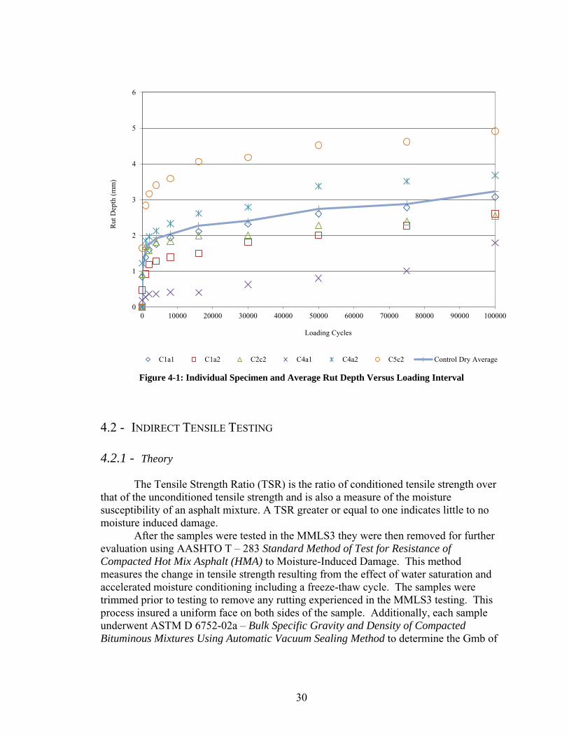
Using Microsoft Excel, the raw deformation data collected for each tested specimen was first zeroed to the initial height reading and reduced to show only the width of the individual specimen. The profilometer measures heights over a set width and may include measurements of the clamps holding the specimen in place and the edges of the tire loading. This data must be eliminated to give an accurate average rut depth reading. In this project a 50 mm width from 80 mm to 130 mm lateral position was chosen through visual analysis of all the profile graphs. After the height data was zeroed to the initial profile reading and the excess measurements were eliminated, the average rut depth from the baseline for each loading interval was calculated and recorded. This procedure was then repeated for each specimen in the MMLS3 test. The average rut depth for each specimen for each loading interval was then complied in a new Microsoft Excel file. Using the rut depths of each specimen from a specific mixture, the overall average rut depth for each loading interval was calculated. This resulting average rut depth was plotted versus loading interval to show the progression in rutting over the duration of the MMLS3 test. The average rut depth values and plots were used for comparison to other mixtures tested with the MMLS3. A sample average rut depth plot is shown in Figure 4-1
30
Figure 4-1: Individual Specimen and Average Rut Depth Versus Loading Interval
4.2 - INDIRECT TENSILE TESTING 4.2.1 - Theory
The Tensile Strength Ratio (TSR) is the ratio of conditioned tensile strength over that of the unconditioned tensile strength and is also a measure of the moisture susceptibility of an asphalt mixture. A TSR greater or equal to one indicates little to no moisture induced damage.
After the samples were tested in the MMLS3 they were then removed for further evaluation using AASHTO T – 283 Standard Method of Test for Resistance of
Compacted Hot Mix Asphalt (HMA) to Moisture-Induced Damage. This method measures the change in tensile strength resulting from the effect of water saturation and accelerated moisture conditioning including a freeze-thaw cycle. The samples were trimmed prior to testing to remove any rutting experienced in the MMLS3 testing. This process insured a uniform face on both sides of the sample. Additionally, each sample underwent ASTM D 6752-02a – Bulk Specific Gravity and Density of Compacted
Bituminous Mixtures Using Automatic Vacuum Sealing Method to determine the Gmb of
0
1
2
3
4
5
6
0 10000 20000 30000 40000 50000 60000 70000 80000 90000 100000
Rut
Dep
th (
mm
)
Loading Cycles
C1a1 C1a2 C2c2 C4a1 C4a2 C5c2 Control Dry Average

31
each compacted specimen. The Gmm from the original mix design and Gmb values obtained from the trimmed samples were then used to calculate the air void content. 4.2.2 - Data Collection
The test was conducted in an INSTRON® universal testing machine where a servo hydraulic actuator applied a constant displacement load at a rate of 50.8 mm/min on the loading strip until the specimen broke. The load was recorded throughout the test by the data acquisition system and the maximum value before the failure of the specimen was then used to calculate the ultimate indirect tensile strength using the following equation;
(1)
Where:
St = indirect tensile strength; P = failure load; Csx = horizontal stress correction factor; ν = Poisson’s ratio; X/Y = ratio of horizontal to vertical deformation. t = thickness of specimen; D = diameter of specimen; Csx = 0.948 − 0.01114 × (t/D) − 0.2693 × ν + 1.436 × (t/D) × ν; ν = −0.1 + 1.480 × (X/Y)2 − 0.778 × (t/D)2 × (X/Y)2
The Figure 4-2 shows the fixture used in the test.
32
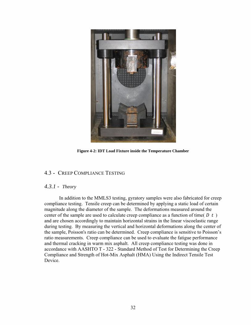
Figure 4-2: IDT Load Fixture inside the Temperature Chamber
4.3 - CREEP COMPLIANCE TESTING 4.3.1 - Theory
In addition to the MMLS3 testing, gyratory samples were also fabricated for creep compliance testing. Tensile creep can be determined by applying a static load of certain magnitude along the diameter of the sample. The deformations measured around the center of the sample are used to calculate creep compliance as a function of time( ) and are chosen accordingly to maintain horizontal strains in the linear viscoelastic range during testing. By measuring the vertical and horizontal deformations along the center of the sample, Poisson's ratio can be determined. Creep compliance is sensitive to Poisson’s
ratio measurements. Creep compliance can be used to evaluate the fatigue performance and thermal cracking in warm mix asphalt. All creep compliance testing was done in accordance with AASHTO T - 322 - Standard Method of Test for Determining the Creep Compliance and Strength of Hot-Mix Asphalt (HMA) Using the Indirect Tensile Test Device.
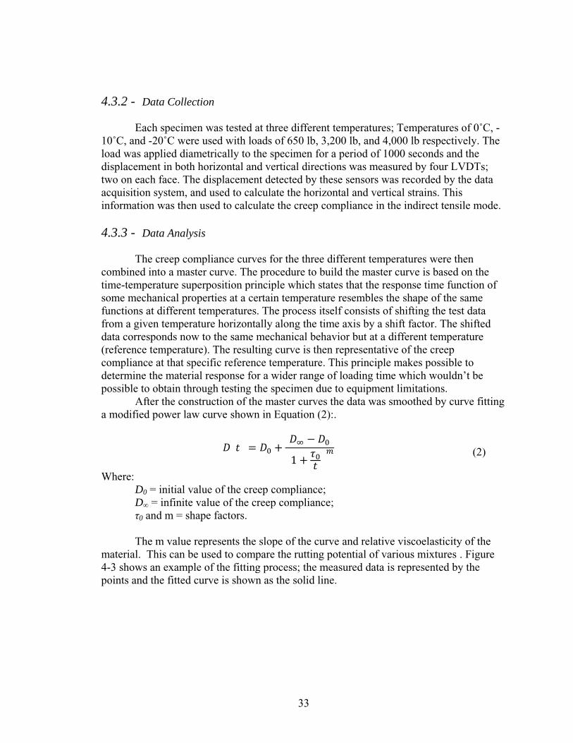
33
4.3.2 - Data Collection
Each specimen was tested at three different temperatures; Temperatures of 0˚C, -10˚C, and -20˚C were used with loads of 650 lb, 3,200 lb, and 4,000 lb respectively. The
load was applied diametrically to the specimen for a period of 1000 seconds and the displacement in both horizontal and vertical directions was measured by four LVDTs; two on each face. The displacement detected by these sensors was recorded by the data acquisition system, and used to calculate the horizontal and vertical strains. This information was then used to calculate the creep compliance in the indirect tensile mode. 4.3.3 - Data Analysis
The creep compliance curves for the three different temperatures were then combined into a master curve. The procedure to build the master curve is based on the time-temperature superposition principle which states that the response time function of some mechanical properties at a certain temperature resembles the shape of the same functions at different temperatures. The process itself consists of shifting the test data from a given temperature horizontally along the time axis by a shift factor. The shifted data corresponds now to the same mechanical behavior but at a different temperature (reference temperature). The resulting curve is then representative of the creep compliance at that specific reference temperature. This principle makes possible to determine the material response for a wider range of loading time which wouldn’t be
possible to obtain through testing the specimen due to equipment limitations. After the construction of the master curves the data was smoothed by curve fitting
a modified power law curve shown in Equation (2):.
(2)
Where: D0 = initial value of the creep compliance; D∞ = infinite value of the creep compliance; τ0 and m = shape factors.
The m value represents the slope of the curve and relative viscoelasticity of the material. This can be used to compare the rutting potential of various mixtures . Figure 4-3 shows an example of the fitting process; the measured data is represented by the points and the fitted curve is shown as the solid line.
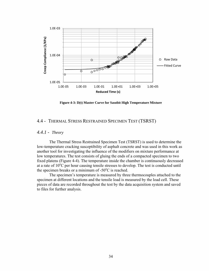
34
Figure 4-3: D(t) Master Curve for Sasobit High Temperature Mixture
4.4 - THERMAL STRESS RESTRAINED SPECIMEN TEST (TSRST) 4.4.1 - Theory
The Thermal Stress Restrained Specimen Test (TSRST) is used to determine the
low-temperature cracking susceptibility of asphalt concrete and was used in this work as another tool for investigating the influence of the modifiers on mixture performance at low temperatures. The test consists of gluing the ends of a compacted specimen to two fixed platens (Figure 4-4). The temperature inside the chamber is continuously decreased at a rate of 10oC per hour causing tensile stresses to develop. The test is conducted until the specimen breaks or a minimum of -50oC is reached.
The specimen’s temperature is measured by three thermocouples attached to the specimen at different locations and the tensile load is measured by the load cell. These pieces of data are recorded throughout the test by the data acquisition system and saved to files for further analysis.
1.0E-05
1.0E-04
1.0E-03
1.0E-05 1.0E-03 1.0E-01 1.0E+01 1.0E+03 1.0E+05
Cre
ep
Co
mp
lian
ce (
1/K
Pa)
Reduced Time (s)
Raw Data
Fitted Curve
35
Figure 4-4: Schematic View of the TSRST Setup
4.4.2 - Data Analysis
Four parameters can be obtained for each test. These parameters are graphically illustrated in Figure 4-5. The fracture strength and fracture temperature are the ultimate stress and temperature recorded by the system before the specimen’s failure. The transition temperature is defined as the temperature where the material changes from viscoelastic to elastic behavior. Below this temperature, thermally induced stresses are not relaxed any longer and the tensile stress follows a linear relationship with
temperature. The slope of the stress temperature curve (T
) is also an important
information and can be used to infer the material behavior at low temperatures. The temperature data was continuously recorded along the test however a data
point reduction was performed and the temperatures used in the analysis were picked at every 0.5oC. The procedure adopted to find the transition temperature consisted in calculating the second derivative of the whole curve. The temperature considered as the transition point was the one where the second derivative changed from zero.
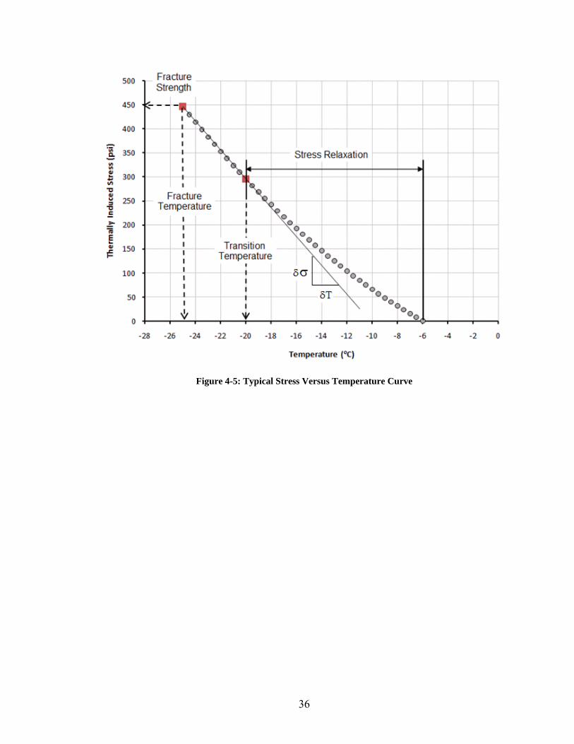
36
Figure 4-5: Typical Stress Versus Temperature Curve

37
4.5 - EXPERIMENTAL PLAN
The experimental plan executed during the course of this work is summarized graphically in the following figures. Figure 4-6 is a schematic view of the tests performed on the test strip field cores and on the plant mix gyratory specimens. Figure 4-7 is a similar schematic for the lab fabricated specimens.
Figure 4-6: Schematic View of the Experimental Plan for Test Strip Field Core and Plant Mix
Gyratory Specimens
TEST STRIP FIELD CORE SPECIMENS TEST STRIP GYRATORY SPECIMENS
MMLS3 MMLS3
European Aspha-minUS Aspha-minCONTROL
WET DRY DRYWET DRYWETWET DRYWET DRYDRYWET
CONTROL US Aspha-min European Aspha-min
50oC Co50
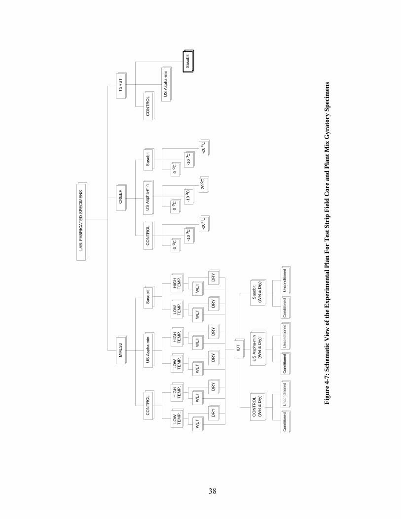
38
LA
B.
FA
BR
ICA
TE
D S
PE
CIM
EN
S
MM
LS
3
IDT
CR
EE
PT
SR
ST
CO
NT
RO
LU
S A
sp
ha
-min
Sa
so
bit
Co
nd
itio
ned
Un
con
ditio
ned
Sa
so
bit
US
Asp
ha
-min
CO
NT
RO
L
CO
NT
RO
LU
S A
sp
ha
-min
Sa
so
bit
0oC
Co
-10
-20
oC
Co
-20
-10
oC
Co
00
oC
Co
-10
-20
oC
CO
NT
RO
L US
Asp
ha
-min
Sa
so
bit
(We
t &
Dry
)(W
et
& D
ry)
(We
t &
Dry
)
Un
con
ditio
ned
Co
nd
itio
ned
Un
con
ditio
ned
Co
nd
itio
ned
LO
WT
EM
P.
TE
MP
.H
IGH
HIG
HT
EM
P.
TE
MP
.L
OW
HIG
HT
EM
P.
TE
MP
.L
OW
WE
T
DR
Y
WE
T
DR
Y
WE
T
DR
Y
WE
T
DR
Y
WE
T
DR
YD
RY
WE
T
Fig
ure
4-7
: S
chem
ati
c V
iew
of
the
Exp
erim
enta
l P
lan
Fo
r T
est
Str
ip F
ield
Co
re a
nd
Pla
nt
Mix
Gy
rato
ry S
pec
imen
s
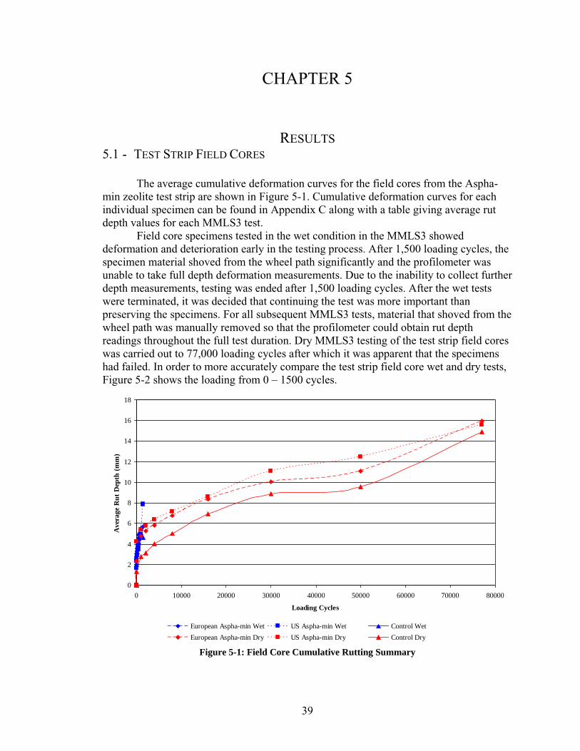
39
CHAPTER 5
RESULTS 5.1 - TEST STRIP FIELD CORES
The average cumulative deformation curves for the field cores from the Aspha-min zeolite test strip are shown in Figure 5-1. Cumulative deformation curves for each individual specimen can be found in Appendix C along with a table giving average rut depth values for each MMLS3 test. Field core specimens tested in the wet condition in the MMLS3 showed deformation and deterioration early in the testing process. After 1,500 loading cycles, the specimen material shoved from the wheel path significantly and the profilometer was unable to take full depth deformation measurements. Due to the inability to collect further depth measurements, testing was ended after 1,500 loading cycles. After the wet tests were terminated, it was decided that continuing the test was more important than preserving the specimens. For all subsequent MMLS3 tests, material that shoved from the wheel path was manually removed so that the profilometer could obtain rut depth readings throughout the full test duration. Dry MMLS3 testing of the test strip field cores was carried out to 77,000 loading cycles after which it was apparent that the specimens had failed. In order to more accurately compare the test strip field core wet and dry tests, Figure 5-2 shows the loading from 0 – 1500 cycles.
Figure 5-1: Field Core Cumulative Rutting Summary
0
2
4
6
8
10
12
14
16
18
0 10000 20000 30000 40000 50000 60000 70000 80000
Loading Cycles
Aver
age
Ru
t D
epth
(m
m)
European Aspha-min Wet US Aspha-min Wet Control Wet
European Aspha-min Dry US Aspha-min Dry Control Dry
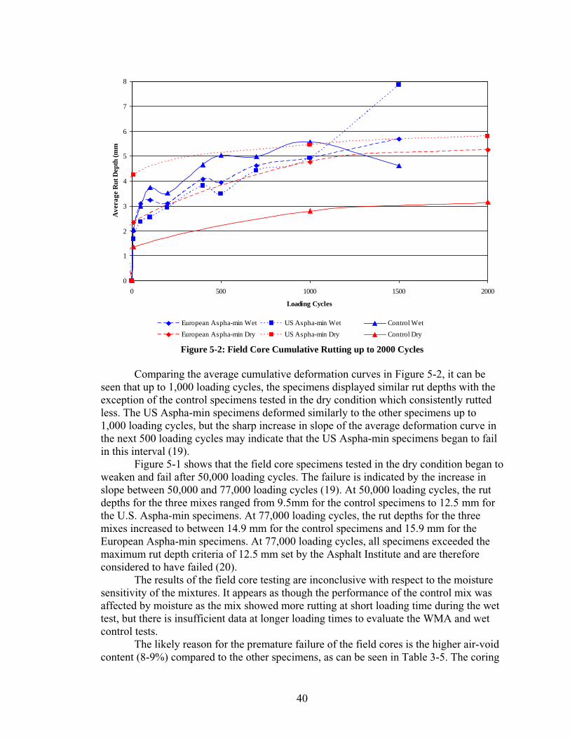
40
Figure 5-2: Field Core Cumulative Rutting up to 2000 Cycles
Comparing the average cumulative deformation curves in Figure 5-2, it can be seen that up to 1,000 loading cycles, the specimens displayed similar rut depths with the exception of the control specimens tested in the dry condition which consistently rutted less. The US Aspha-min specimens deformed similarly to the other specimens up to 1,000 loading cycles, but the sharp increase in slope of the average deformation curve in the next 500 loading cycles may indicate that the US Aspha-min specimens began to fail in this interval (19). Figure 5-1 shows that the field core specimens tested in the dry condition began to weaken and fail after 50,000 loading cycles. The failure is indicated by the increase in slope between 50,000 and 77,000 loading cycles (19). At 50,000 loading cycles, the rut depths for the three mixes ranged from 9.5mm for the control specimens to 12.5 mm for the U.S. Aspha-min specimens. At 77,000 loading cycles, the rut depths for the three mixes increased to between 14.9 mm for the control specimens and 15.9 mm for the European Aspha-min specimens. At 77,000 loading cycles, all specimens exceeded the maximum rut depth criteria of 12.5 mm set by the Asphalt Institute and are therefore considered to have failed (20). The results of the field core testing are inconclusive with respect to the moisture sensitivity of the mixtures. It appears as though the performance of the control mix was affected by moisture as the mix showed more rutting at short loading time during the wet test, but there is insufficient data at longer loading times to evaluate the WMA and wet control tests. The likely reason for the premature failure of the field cores is the higher air-void content (8-9%) compared to the other specimens, as can be seen in Table 3-5. The coring
0
1
2
3
4
5
6
7
8
0 500 1000 1500 2000
Loading Cycles
Av
era
ge R
ut
Dep
th (
mm
)
European Aspha-min Wet US Aspha-min Wet Control Wet
European Aspha-min Dry US Aspha-min Dry Control Dry
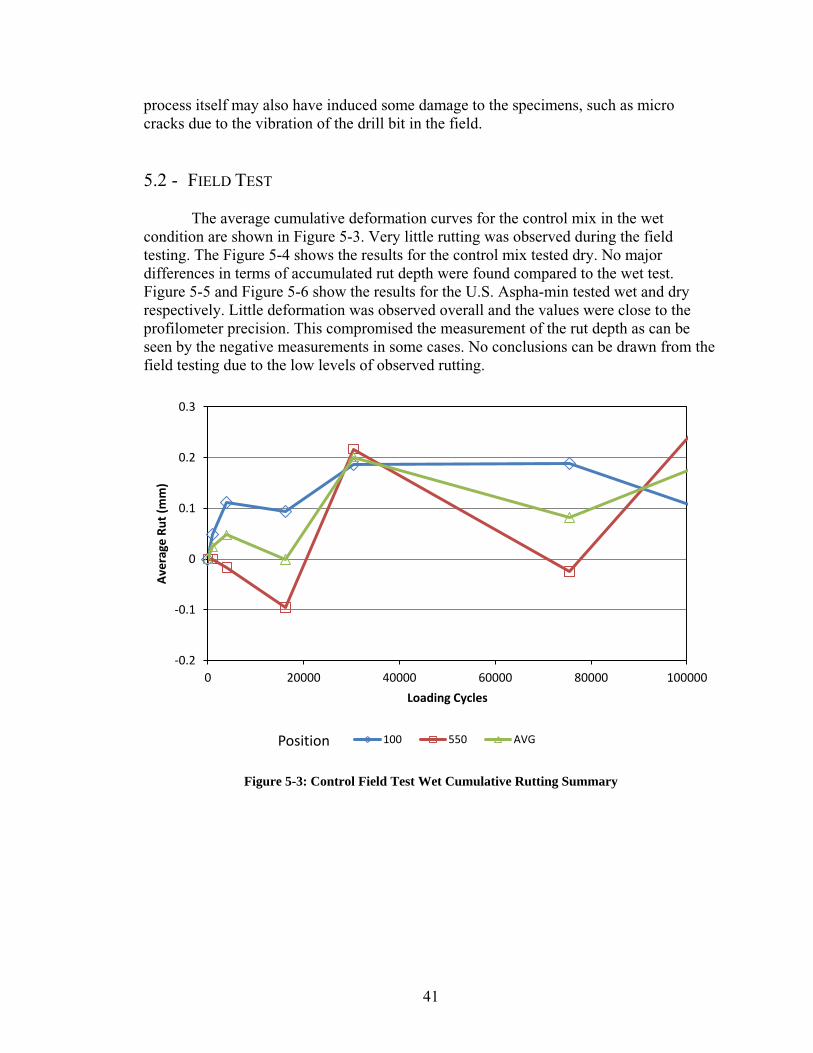
41
process itself may also have induced some damage to the specimens, such as micro cracks due to the vibration of the drill bit in the field. 5.2 - FIELD TEST
The average cumulative deformation curves for the control mix in the wet condition are shown in Figure 5-3. Very little rutting was observed during the field testing. The Figure 5-4 shows the results for the control mix tested dry. No major differences in terms of accumulated rut depth were found compared to the wet test. Figure 5-5 and Figure 5-6 show the results for the U.S. Aspha-min tested wet and dry respectively. Little deformation was observed overall and the values were close to the profilometer precision. This compromised the measurement of the rut depth as can be seen by the negative measurements in some cases. No conclusions can be drawn from the field testing due to the low levels of observed rutting.
Figure 5-3: Control Field Test Wet Cumulative Rutting Summary
-0.2
-0.1
0
0.1
0.2
0.3
0 20000 40000 60000 80000 100000
Ave
rage
Ru
t (m
m)
Loading Cycles
Position 100 550 AVG
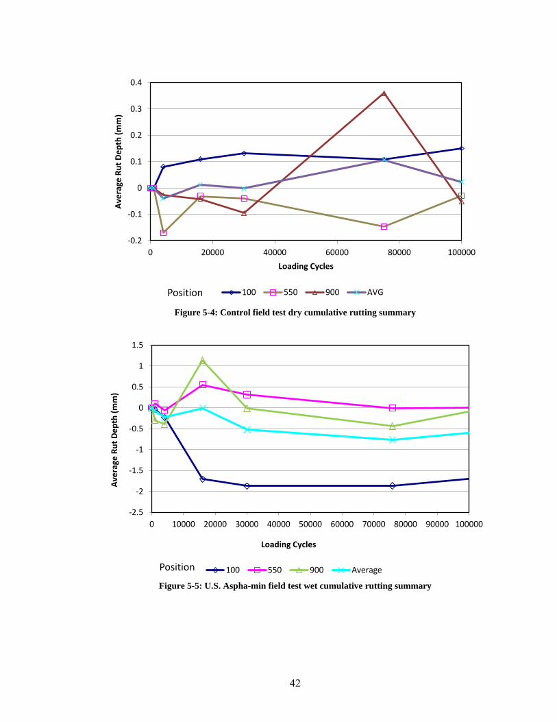
42
Figure 5-4: Control field test dry cumulative rutting summary
Figure 5-5: U.S. Aspha-min field test wet cumulative rutting summary
-0.2
-0.1
0
0.1
0.2
0.3
0.4
0 20000 40000 60000 80000 100000
Ave
rage
Ru
t D
ep
th (
mm
)
Loading Cycles
Position 100 550 900 AVG
-2.5
-2
-1.5
-1
-0.5
0
0.5
1
1.5
0 10000 20000 30000 40000 50000 60000 70000 80000 90000 100000
Ave
rage
Ru
t D
ep
th (
mm
)
Loading Cycles
Position 100 550 900 Average
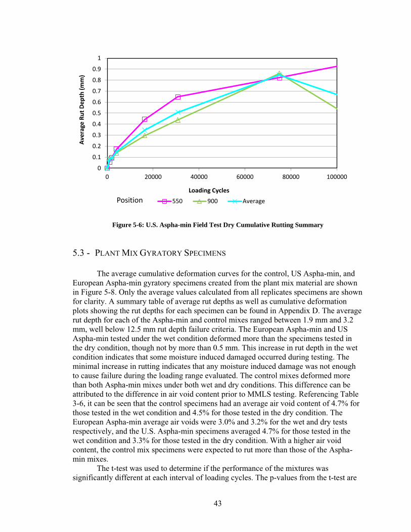
43
Figure 5-6: U.S. Aspha-min Field Test Dry Cumulative Rutting Summary
5.3 - PLANT MIX GYRATORY SPECIMENS
The average cumulative deformation curves for the control, US Aspha-min, and European Aspha-min gyratory specimens created from the plant mix material are shown in Figure 5-8. Only the average values calculated from all replicates specimens are shown for clarity. A summary table of average rut depths as well as cumulative deformation plots showing the rut depths for each specimen can be found in Appendix D. The average rut depth for each of the Aspha-min and control mixes ranged between 1.9 mm and 3.2 mm, well below 12.5 mm rut depth failure criteria. The European Aspha-min and US Aspha-min tested under the wet condition deformed more than the specimens tested in the dry condition, though not by more than 0.5 mm. This increase in rut depth in the wet condition indicates that some moisture induced damaged occurred during testing. The minimal increase in rutting indicates that any moisture induced damage was not enough to cause failure during the loading range evaluated. The control mixes deformed more than both Aspha-min mixes under both wet and dry conditions. This difference can be attributed to the difference in air void content prior to MMLS testing. Referencing Table 3-6, it can be seen that the control specimens had an average air void content of 4.7% for those tested in the wet condition and 4.5% for those tested in the dry condition. The European Aspha-min average air voids were 3.0% and 3.2% for the wet and dry tests respectively, and the U.S. Aspha-min specimens averaged 4.7% for those tested in the wet condition and 3.3% for those tested in the dry condition. With a higher air void content, the control mix specimens were expected to rut more than those of the Aspha-min mixes. The t-test was used to determine if the performance of the mixtures was significantly different at each interval of loading cycles. The p-values from the t-test are
0
0.1
0.2
0.3
0.4
0.5
0.6
0.7
0.8
0.9
1
0 20000 40000 60000 80000 100000
Ave
rage
Ru
t D
ep
th (
mm
)
Loading Cycles
Position 550 900 Average
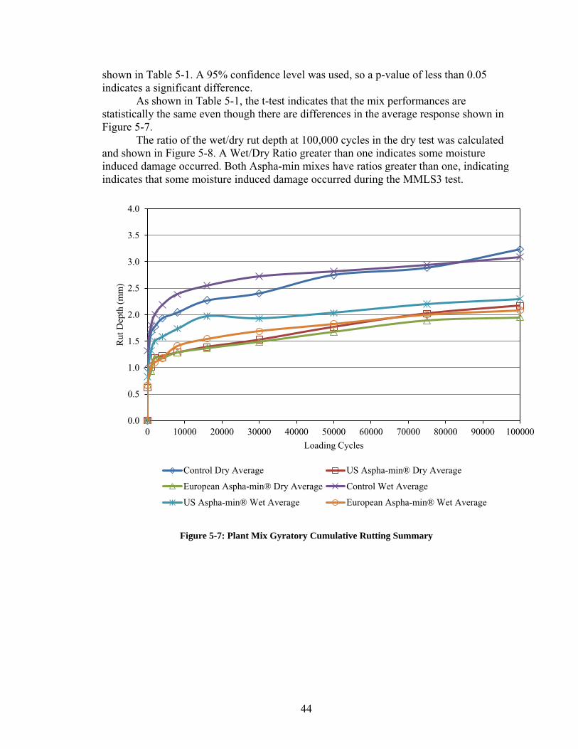
44
shown in Table 5-1. A 95% confidence level was used, so a p-value of less than 0.05 indicates a significant difference. As shown in Table 5-1, the t-test indicates that the mix performances are statistically the same even though there are differences in the average response shown in Figure 5-7. The ratio of the wet/dry rut depth at 100,000 cycles in the dry test was calculated and shown in Figure 5-8. A Wet/Dry Ratio greater than one indicates some moisture induced damage occurred. Both Aspha-min mixes have ratios greater than one, indicating indicates that some moisture induced damage occurred during the MMLS3 test.
Figure 5-7: Plant Mix Gyratory Cumulative Rutting Summary
0.0
0.5
1.0
1.5
2.0
2.5
3.0
3.5
4.0
0 10000 20000 30000 40000 50000 60000 70000 80000 90000 100000
Rut
Dep
th (
mm
)
Loading Cycles
Control Dry Average US Aspha-min® Dry Average
European Aspha-min® Dry Average Control Wet Average
US Aspha-min® Wet Average European Aspha-min® Wet Average
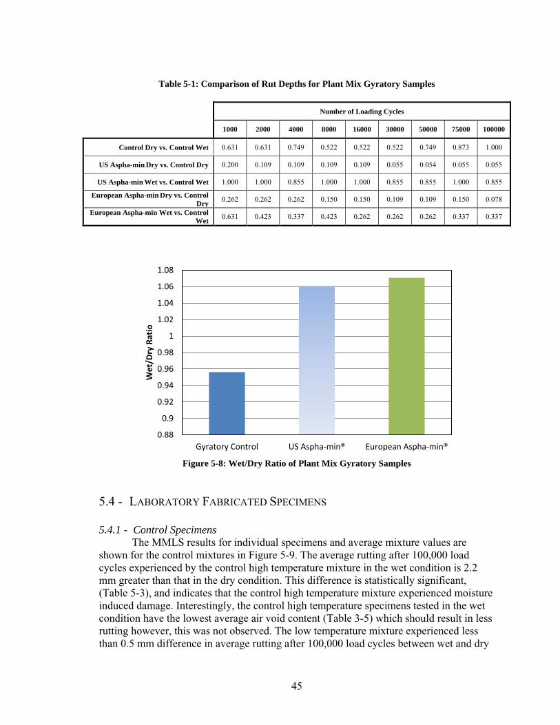
45
Table 5-1: Comparison of Rut Depths for Plant Mix Gyratory Samples
Number of Loading Cycles
1000 2000 4000 8000 16000 30000 50000 75000 100000
Control Dry vs. Control Wet 0.631 0.631 0.749 0.522 0.522 0.522 0.749 0.873 1.000
US Aspha-min Dry vs. Control Dry 0.200 0.109 0.109 0.109 0.109 0.055 0.054 0.055 0.055
US Aspha-min Wet vs. Control Wet 1.000 1.000 0.855 1.000 1.000 0.855 0.855 1.000 0.855
European Aspha-min Dry vs. Control
Dry 0.262 0.262 0.262 0.150 0.150 0.109 0.109 0.150 0.078
European Aspha-min Wet vs. Control
Wet 0.631 0.423 0.337 0.423 0.262 0.262 0.262 0.337 0.337
Figure 5-8: Wet/Dry Ratio of Plant Mix Gyratory Samples
5.4 - LABORATORY FABRICATED SPECIMENS 5.4.1 - Control Specimens
The MMLS results for individual specimens and average mixture values are shown for the control mixtures in Figure 5-9. The average rutting after 100,000 load cycles experienced by the control high temperature mixture in the wet condition is 2.2 mm greater than that in the dry condition. This difference is statistically significant, (Table 5-3), and indicates that the control high temperature mixture experienced moisture induced damage. Interestingly, the control high temperature specimens tested in the wet condition have the lowest average air void content (Table 3-5) which should result in less rutting however, this was not observed. The low temperature mixture experienced less than 0.5 mm difference in average rutting after 100,000 load cycles between wet and dry
0.88
0.9
0.92
0.94
0.96
0.98
1
1.02
1.04
1.06
1.08
Gyratory Control US Aspha-min® European Aspha-min®
We
t/D
ry R
atio
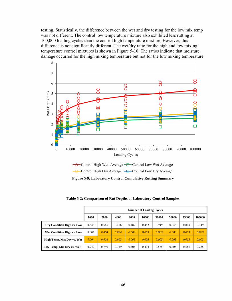
46
testing. Statistically, the difference between the wet and dry testing for the low mix temp was not different. The control low temperature mixture also exhibited less rutting at 100,000 loading cycles than the control high temperature mixture. However, this difference is not significantly different. The wet/dry ratio for the high and low mixing temperature control mixtures is shown in Figure 5-10. The ratios indicate that moisture damage occurred for the high mixing temperature but not for the low mixing temperature.
Figure 5-9: Laboratory Control Cumulative Rutting Summary
Table 5-2: Comparison of Rut Depths of Laboratory Control Samples
Number of Loading Cycles
1000 2000 4000 8000 16000 30000 50000 75000 100000
Dry Condition High vs. Low 0.848 0.565 0.406 0.482 0.482 0.949 0.848 0.848 0.749
Wet Condition High vs. Low 0.007 0.004 0.004 0.003 0.003 0.003 0.003 0.003 0.003
High Temp. Mix Dry vs. Wet 0.004 0.004 0.003 0.003 0.003 0.003 0.003 0.003 0.003
Low Temp. Mix Dry vs. Wet 0.949 0.749 0.749 0.406 0.494 0.565 0.406 0.565 0.225
0
1
2
3
4
5
6
7
8
0 10000 20000 30000 40000 50000 60000 70000 80000 90000 100000
Rut
Dep
th (
mm
)
Loading Cycles
Control High Wet Average Control Low Wet Average
Control High Dry Average Control Low Dry Average
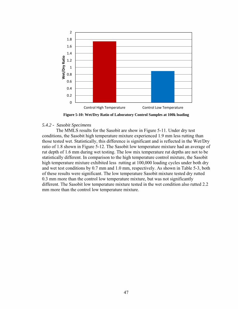
47
Figure 5-10: Wet/Dry Ratio of Laboratory Control Samples at 100k loading
5.4.2 - Sasobit Specimens
The MMLS results for the Sasobit are show in Figure 5-11. Under dry test conditions, the Sasobit high temperature mixture experienced 1.9 mm less rutting than those tested wet. Statistically, this difference is significant and is reflected in the Wet/Dry ratio of 1.8 shown in Figure 5-12. The Sasobit low temperature mixture had an average of rut depth of 1.6 mm during wet testing. The low mix temperature rut depths are not to be statistically different. In comparison to the high temperature control mixture, the Sasobit high temperature mixture exhibited less rutting at 100,000 loading cycles under both dry and wet test conditions by 0.7 mm and 1.0 mm, respectively. As shown in Table 5-3, both of these results were significant. The low temperature Sasobit mixture tested dry rutted 0.3 mm more than the control low temperature mixture, but was not significantly different. The Sasobit low temperature mixture tested in the wet condition also rutted 2.2 mm more than the control low temperature mixture.
0
0.2
0.4
0.6
0.8
1
1.2
1.4
1.6
1.8
2
Control High Temperature Control Low Temperature
We
t/D
ry R
atio

48
Figure 5-11: Laboratory Sasobit Cumulative Rutting Summary
Table 5-3: Comparison of Rut Depths of Sasobit Mixtures
Number of Loading Cycles
1000 2000 4000 8000 16000 30000 50000 75000 100000
Control vs. Sasobit: High Dry 0.009 0.018 0.018 0.048 0.110 0.180 0.085 0.048 0.048
Control vs. Sasobit: Low Dry 0.180 0.225 0.482 0.749 0.110 0.085 0.110 0.338 0.225
Control vs. Sasobit: High Wet 0.038 0.046 0.046 0.046 0.022 0.007 0.010 0.016 0.022
Control vs. Sasobit: Low Wet 0.242 0.143 0.143 0.143 0.079 0.079 0.040 0.040 0.040
High Temp. Sasobit Dry vs. Wet 0.006 0.006 0.006 0.006 0.009 0.009 0.003 0.003 0.002
Low Temp. Sasobit Dry vs. Wet 0.079 0.079 0.079 0.079 0.079 0.242 0.143 0.242 0.143
0
1
2
3
4
5
6
7
8
0 10000 20000 30000 40000 50000 60000 70000 80000 90000 100000
Rut
Dep
th (
mm
)
Loading Cycles
Sasobit® High Wet Average Sasobit® Low Wet Average
Sasobit® High Dry Average Sasobit® Low Dry Average
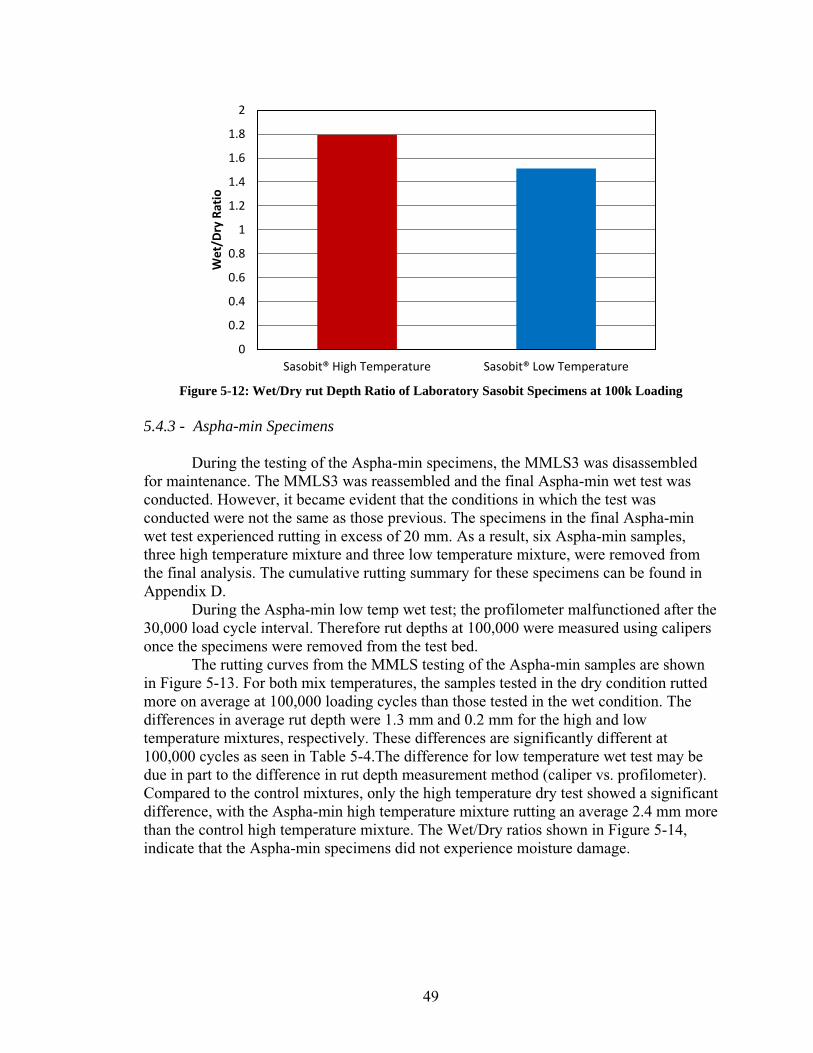
49
Figure 5-12: Wet/Dry rut Depth Ratio of Laboratory Sasobit Specimens at 100k Loading
5.4.3 - Aspha-min Specimens
During the testing of the Aspha-min specimens, the MMLS3 was disassembled for maintenance. The MMLS3 was reassembled and the final Aspha-min wet test was conducted. However, it became evident that the conditions in which the test was conducted were not the same as those previous. The specimens in the final Aspha-min wet test experienced rutting in excess of 20 mm. As a result, six Aspha-min samples, three high temperature mixture and three low temperature mixture, were removed from the final analysis. The cumulative rutting summary for these specimens can be found in Appendix D.
During the Aspha-min low temp wet test; the profilometer malfunctioned after the 30,000 load cycle interval. Therefore rut depths at 100,000 were measured using calipers once the specimens were removed from the test bed.
The rutting curves from the MMLS testing of the Aspha-min samples are shown in Figure 5-13. For both mix temperatures, the samples tested in the dry condition rutted more on average at 100,000 loading cycles than those tested in the wet condition. The differences in average rut depth were 1.3 mm and 0.2 mm for the high and low temperature mixtures, respectively. These differences are significantly different at 100,000 cycles as seen in Table 5-4.The difference for low temperature wet test may be due in part to the difference in rut depth measurement method (caliper vs. profilometer). Compared to the control mixtures, only the high temperature dry test showed a significant difference, with the Aspha-min high temperature mixture rutting an average 2.4 mm more than the control high temperature mixture. The Wet/Dry ratios shown in Figure 5-14, indicate that the Aspha-min specimens did not experience moisture damage.
0
0.2
0.4
0.6
0.8
1
1.2
1.4
1.6
1.8
2
Sasobit® High Temperature Sasobit® Low Temperature
We
t/D
ry R
atio
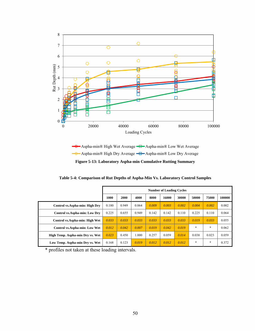
50
Figure 5-13: Laboratory Aspha-min Cumulative Rutting Summary
Table 5-4: Comparison of Rut Depths of Aspha-Min Vs. Laboratory Control Samples
Number of Loading Cycles
1000 2000 4000 8000 16000 30000 50000 75000 100000
Control vs.Aspha-min: High Dry 0.180 0.949 0.064 0.009 0.003 0.002 0.004 0.002 0.002
Control vs.Aspha-min: Low Dry 0.225 0.655 0.949 0.142 0.142 0.110 0.225 0.110 0.064
Control vs.Aspha-min: High Wet 0.033 0.033 0.033 0.033 0.033 0.033 0.019 0.033 0.055
Control vs.Aspha-min: Low Wet 0.012 0.042 0.007 0.019 0.042 0.019 * * 0.062
High Temp. Aspha-min Dry vs. Wet 0.023 0.450 1.000 0.257 0.059 0.014 0.038 0.023 0.059
Low Temp. Aspha-min Dry vs. Wet 0.168 0.123 0.019 0.012 0.012 0.012 * * 0.372
* profiles not taken at these loading intervals.
0
1
2
3
4
5
6
7
8
0 20000 40000 60000 80000 100000
Rut
Dep
th (
mm
)
Loading Cycles
Aspha-min® High Wet Average Aspha-min® Low Wet Average
Aspha-min® High Dry Average Aspha-min® Low Dry Average
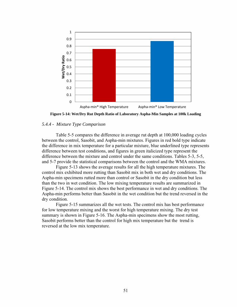
51
Figure 5-14: Wet/Dry Rut Depth Ratio of Laboratory Aspha-Min Samples at 100k Loading
5.4.4 - Mixture Type Comparison
Table 5-5 compares the difference in average rut depth at 100,000 loading cycles between the control, Sasobit, and Aspha-min mixtures. Figures in red bold type indicate the difference in mix temperature for a particular mixture, blue underlined type represents difference between test conditions, and figures in green italicized type represent the difference between the mixture and control under the same conditions. Tables 5-3, 5-5, and 5-7 provide the statistical comparisons between the control and the WMA mixtures.
Figure 5-13 shows the average results for all the high temperature mixtures. The control mix exhibited more rutting than Sasobit mix in both wet and dry conditions. The Aspha-min specimens rutted more than control or Sasobit in the dry condition but less than the two in wet condition. The low mixing temperature results are summarized in Figure 5-14. The control mix shows the best performance in wet and dry conditions. The Aspha-min performs better than Sasobit in the wet condition but the trend reversed in the dry condition.
Figure 5-15 summarizes all the wet tests. The control mix has best performance for low temperature mixing and the worst for high temperature mixing. The dry test summary is shown in Figure 5-16. The Aspha-min specimens show the most rutting, Sasobit performs better than the control for high mix temperature but the trend is reversed at the low mix temperature.
0
0.1
0.2
0.3
0.4
0.5
0.6
0.7
0.8
0.9
1
Aspha-min® High Temperature Aspha-min® Low Temperature
We
t/D
ry R
atio
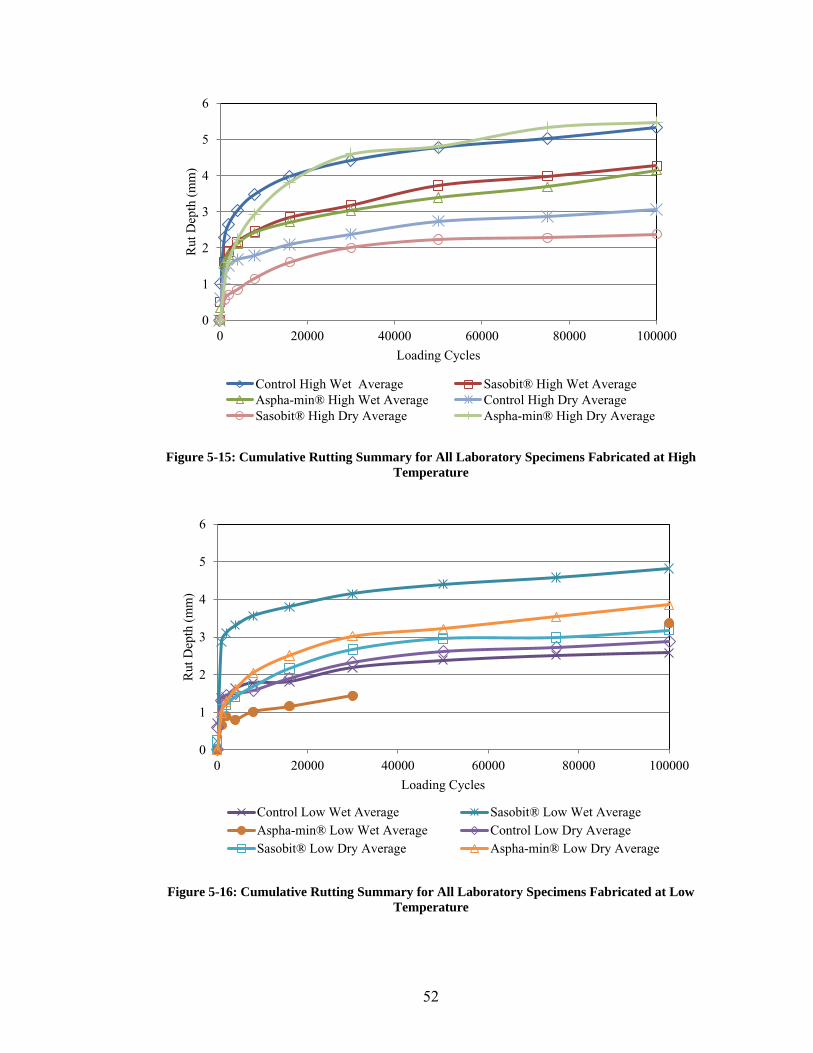
52
Figure 5-15: Cumulative Rutting Summary for All Laboratory Specimens Fabricated at High
Temperature
Figure 5-16: Cumulative Rutting Summary for All Laboratory Specimens Fabricated at Low
Temperature
0
1
2
3
4
5
6
0 20000 40000 60000 80000 100000
Rut
Dep
th (
mm
)
Loading Cycles
Control High Wet Average Sasobit® High Wet AverageAspha-min® High Wet Average Control High Dry AverageSasobit® High Dry Average Aspha-min® High Dry Average
0
1
2
3
4
5
6
0 20000 40000 60000 80000 100000
Rut
Dep
th (
mm
)
Loading Cycles
Control Low Wet Average Sasobit® Low Wet AverageAspha-min® Low Wet Average Control Low Dry AverageSasobit® Low Dry Average Aspha-min® Low Dry Average
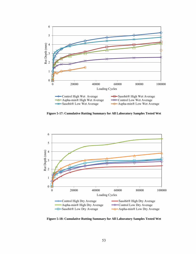
53
Figure 5-17: Cumulative Rutting Summary for All Laboratory Samples Tested Wet
Figure 5-18: Cumulative Rutting Summary for All Laboratory Samples Tested Wet
0
1
2
3
4
5
6
0 20000 40000 60000 80000 100000
Rut
Dep
th (
mm
)
Loading Cycles
Control High Wet Average Sasobit® High Wet AverageAspha-min® High Wet Average Control Low Wet AverageSasobit® Low Wet Average Aspha-min® Low Wet Average
0
1
2
3
4
5
6
0 20000 40000 60000 80000 100000
Rut
Dep
th (
mm
)
Loading Cycles
Control High Dry Average Sasobit® High Dry AverageAspha-min® High Dry Average Control Low Dry AverageSasobit® Low Dry Average Aspha-min® Low Dry Average
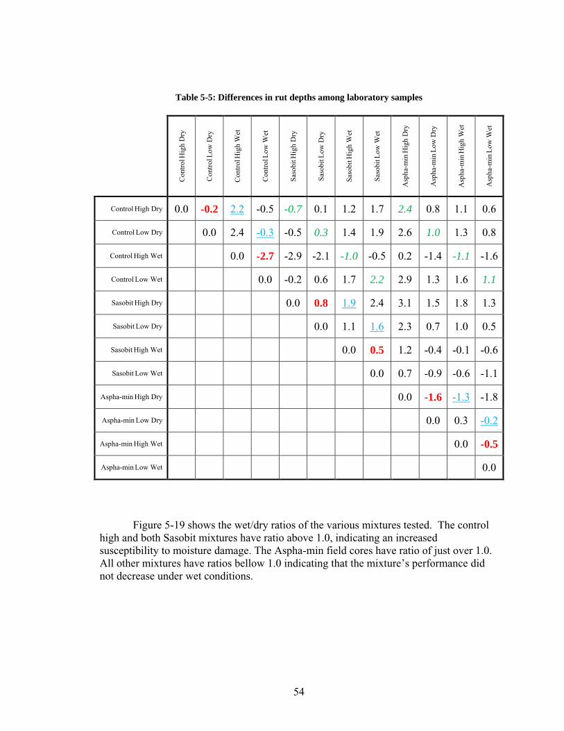
54
Table 5-5: Differences in rut depths among laboratory samples
Con
trol
Hig
h D
ry
Con
trol
Low
Dry
Con
trol
Hig
h W
et
Con
trol
Low
Wet
Saso
bit H
igh
Dry
Saso
bit L
ow D
ry
Saso
bit H
igh
Wet
Saso
bit L
ow W
et
Asp
ha-m
in H
igh
Dry
Asp
ha-m
in L
ow D
ry
Asp
ha-m
in H
igh
Wet
Asp
ha-m
in L
ow W
et
Control High Dry 0.0 -0.2 2.2 -0.5 -0.7 0.1 1.2 1.7 2.4 0.8 1.1 0.6
Control Low Dry 0.0 2.4 -0.3 -0.5 0.3 1.4 1.9 2.6 1.0 1.3 0.8
Control High Wet 0.0 -2.7 -2.9 -2.1 -1.0 -0.5 0.2 -1.4 -1.1 -1.6
Control Low Wet 0.0 -0.2 0.6 1.7 2.2 2.9 1.3 1.6 1.1
Sasobit High Dry 0.0 0.8 1.9 2.4 3.1 1.5 1.8 1.3
Sasobit Low Dry 0.0 1.1 1.6 2.3 0.7 1.0 0.5
Sasobit High Wet 0.0 0.5 1.2 -0.4 -0.1 -0.6
Sasobit Low Wet 0.0 0.7 -0.9 -0.6 -1.1
Aspha-min High Dry 0.0 -1.6 -1.3 -1.8
Aspha-min Low Dry 0.0 0.3 -0.2
Aspha-min High Wet 0.0 -0.5
Aspha-min Low Wet 0.0
Figure 5-19 shows the wet/dry ratios of the various mixtures tested. The control
high and both Sasobit mixtures have ratio above 1.0, indicating an increased susceptibility to moisture damage. The Aspha-min field cores have ratio of just over 1.0. All other mixtures have ratios bellow 1.0 indicating that the mixture’s performance did not decrease under wet conditions.
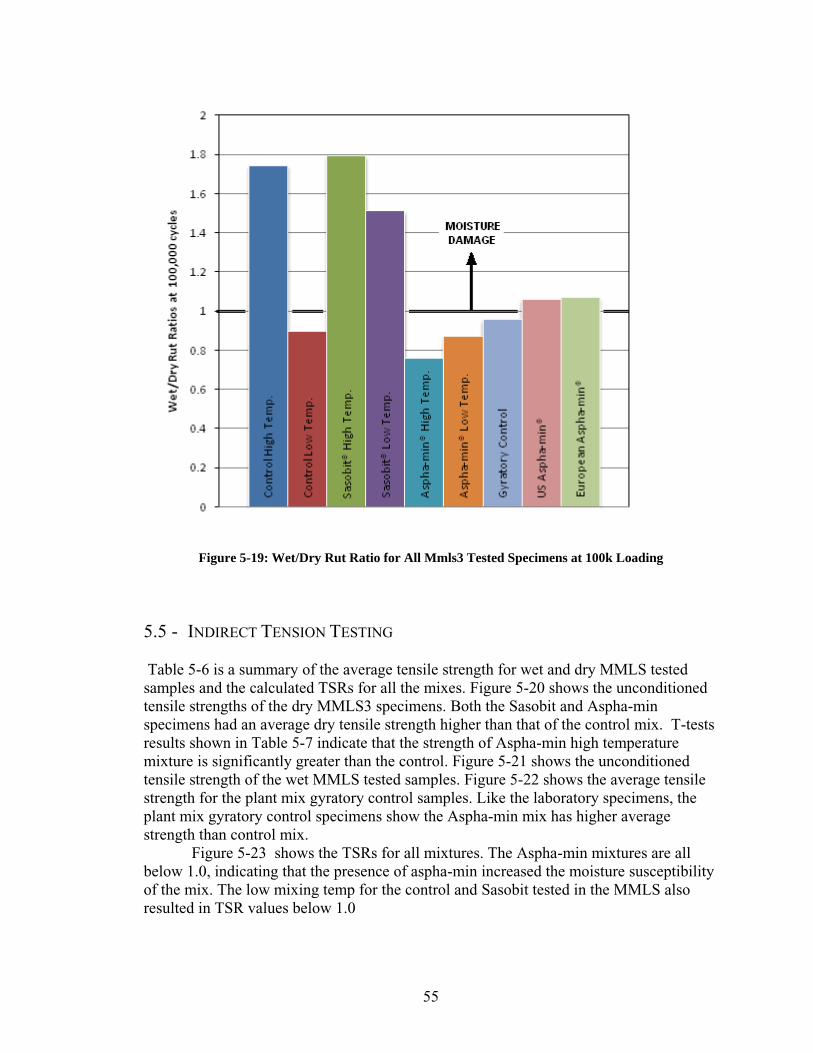
55
Figure 5-19: Wet/Dry Rut Ratio for All Mmls3 Tested Specimens at 100k Loading
5.5 - INDIRECT TENSION TESTING Table 5-6 is a summary of the average tensile strength for wet and dry MMLS tested samples and the calculated TSRs for all the mixes. Figure 5-20 shows the unconditioned tensile strengths of the dry MMLS3 specimens. Both the Sasobit and Aspha-min specimens had an average dry tensile strength higher than that of the control mix. T-tests results shown in Table 5-7 indicate that the strength of Aspha-min high temperature mixture is significantly greater than the control. Figure 5-21 shows the unconditioned tensile strength of the wet MMLS tested samples. Figure 5-22 shows the average tensile strength for the plant mix gyratory control samples. Like the laboratory specimens, the plant mix gyratory control specimens show the Aspha-min mix has higher average strength than control mix. Figure 5-23 shows the TSRs for all mixtures. The Aspha-min mixtures are all below 1.0, indicating that the presence of aspha-min increased the moisture susceptibility of the mix. The low mixing temp for the control and Sasobit tested in the MMLS also resulted in TSR values below 1.0
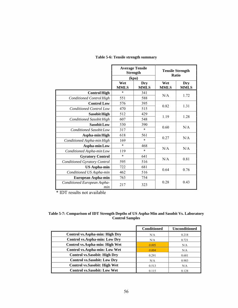
56
Table 5-6: Tensile strength summary
Average Tensile
Strength Tensile Strength
Ratio
(kpa)
Wet
MMLS
Dry
MMLS
Wet
MMLS
Dry
MMLS
Control High * 341
N/A 1.72 Conditioned Control High 551 588
Control Low 576 395 0.82 1.31
Conditioned Control Low 470 515 Sasobit
High 512 429
1.19 1.28 Conditioned Sasobit High 607 548
Sasobit Low 530 390
0.60 N/A Conditioned Sasobit Low 317 *
Aspha-min High 618 561
0.27 N/A Conditioned Aspha-min High 169 *
Aspha-min Low * 468
N/A N/A Conditioned Aspha-min Low 119 *
Gyratory Control * 641 N/A 0.81
Conditioned Gyratory Control 595 516 US Aspha-min 722 681
0.64 0.76 Conditioned US Aspha-min 462 516
European Aspha-min 763 754 0.28 0.43 Conditioned European Aspha-
min 217 323
* IDT results not available
Table 5-7: Comparison of IDT Strength Depths of US Aspha-Min and Sasobit Vs. Laboratory
Control Samples
Conditioned Unconditioned
Control vs.Aspha-min: High Dry N/A 0.218
Control vs.Aspha-min: Low Dry N/A 0.721
Control vs.Aspha-min: High Wet 0.005 N/A
Control vs.Aspha-min: Low Wet 0.004 N/A
Control vs.Sasobit: High Dry 0.291 0.681
Control vs.Sasobit: Low Dry N/A 0.983
Control vs.Sasobit: High Wet 0.513 N/A
Control vs.Sasobit: Low Wet 0.115 0.128
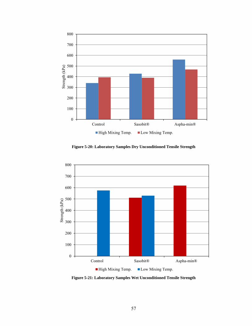
57
Figure 5-20: Laboratory Samples Dry Unconditioned Tensile Strength
Figure 5-21: Laboratory Samples Wet Unconditioned Tensile Strength
0
100
200
300
400
500
600
700
800
Control Sasobit® Aspha-min®
Stre
ngth
(kP
a)
High Mixing Temp. Low Mixing Temp.
0
100
200
300
400
500
600
700
800
Control Sasobit® Aspha-min®
Stre
ngth
(kP
a)
High Mixing Temp. Low Mixing Temp.
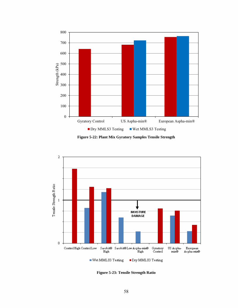
58
Figure 5-22: Plant Mix Gyratory Samples Tensile Strength
Figure 5-23: Tensile Strength Ratio
0
100
200
300
400
500
600
700
800
Gyratory Control US Aspha-min® European Aspha-min®
Stre
ngth
(kP
a)
Dry MMLS3 Testing Wet MMLS3 Testing
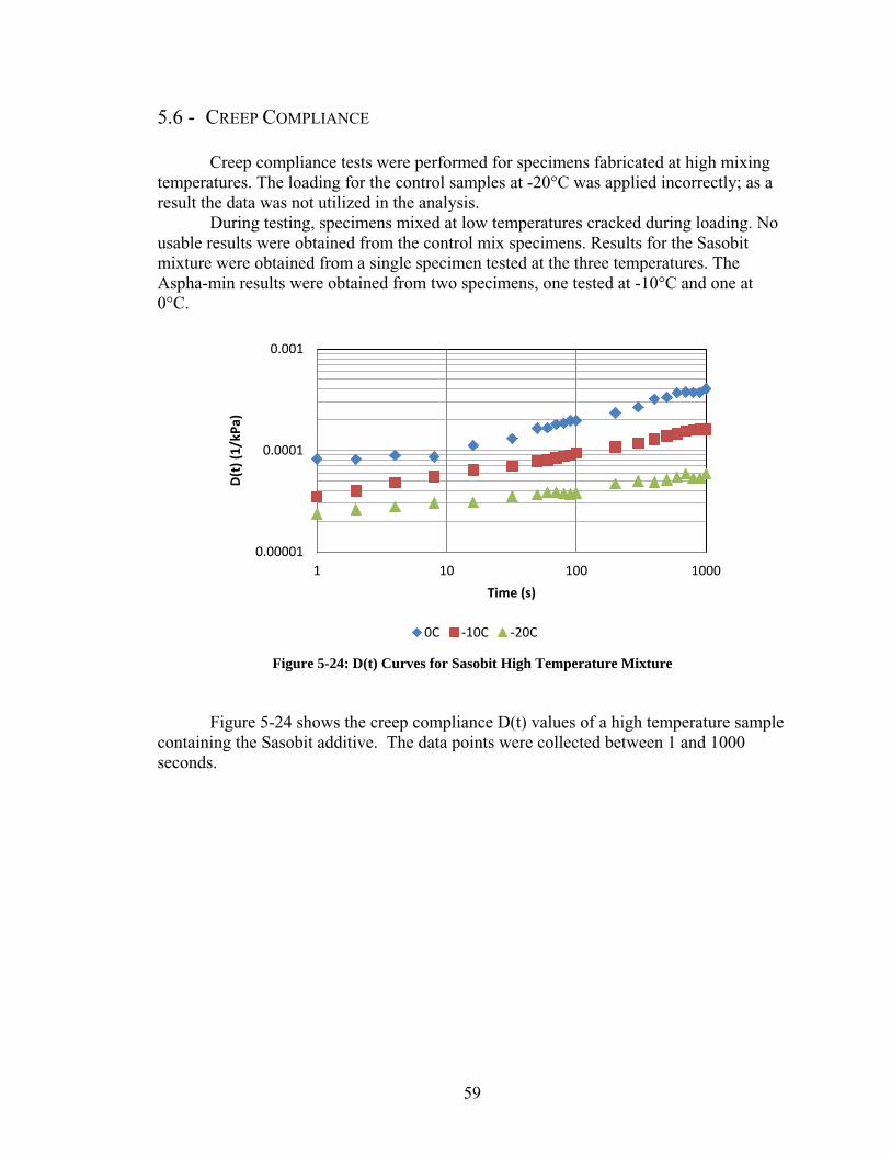
59
5.6 - CREEP COMPLIANCE
Creep compliance tests were performed for specimens fabricated at high mixing temperatures. The loading for the control samples at -20°C was applied incorrectly; as a result the data was not utilized in the analysis.
During testing, specimens mixed at low temperatures cracked during loading. No usable results were obtained from the control mix specimens. Results for the Sasobit mixture were obtained from a single specimen tested at the three temperatures. The Aspha-min results were obtained from two specimens, one tested at -10°C and one at 0°C.
Figure 5-24: D(t) Curves for Sasobit High Temperature Mixture
Figure 5-24 shows the creep compliance D(t) values of a high temperature sample containing the Sasobit additive. The data points were collected between 1 and 1000 seconds.
0.00001
0.0001
0.001
1 10 100 1000
D(t
) (1
/kP
a)
Time (s)
0C -10C -20C
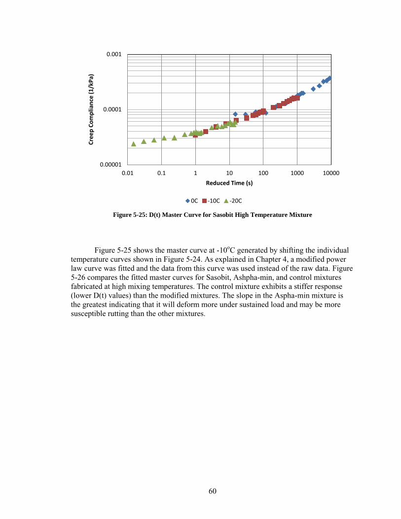
60
Figure 5-25: D(t) Master Curve for Sasobit High Temperature Mixture
Figure 5-25 shows the master curve at -10oC generated by shifting the individual
temperature curves shown in Figure 5-24. As explained in Chapter 4, a modified power law curve was fitted and the data from this curve was used instead of the raw data. Figure 5-26 compares the fitted master curves for Sasobit, Ashpha-min, and control mixtures fabricated at high mixing temperatures. The control mixture exhibits a stiffer response (lower D(t) values) than the modified mixtures. The slope in the Aspha-min mixture is the greatest indicating that it will deform more under sustained load and may be more susceptible rutting than the other mixtures.
0.00001
0.0001
0.001
0.01 0.1 1 10 100 1000 10000
Cre
ep
Co
mp
lian
ce (
1/k
Pa)
Reduced Time (s)
0C -10C -20C
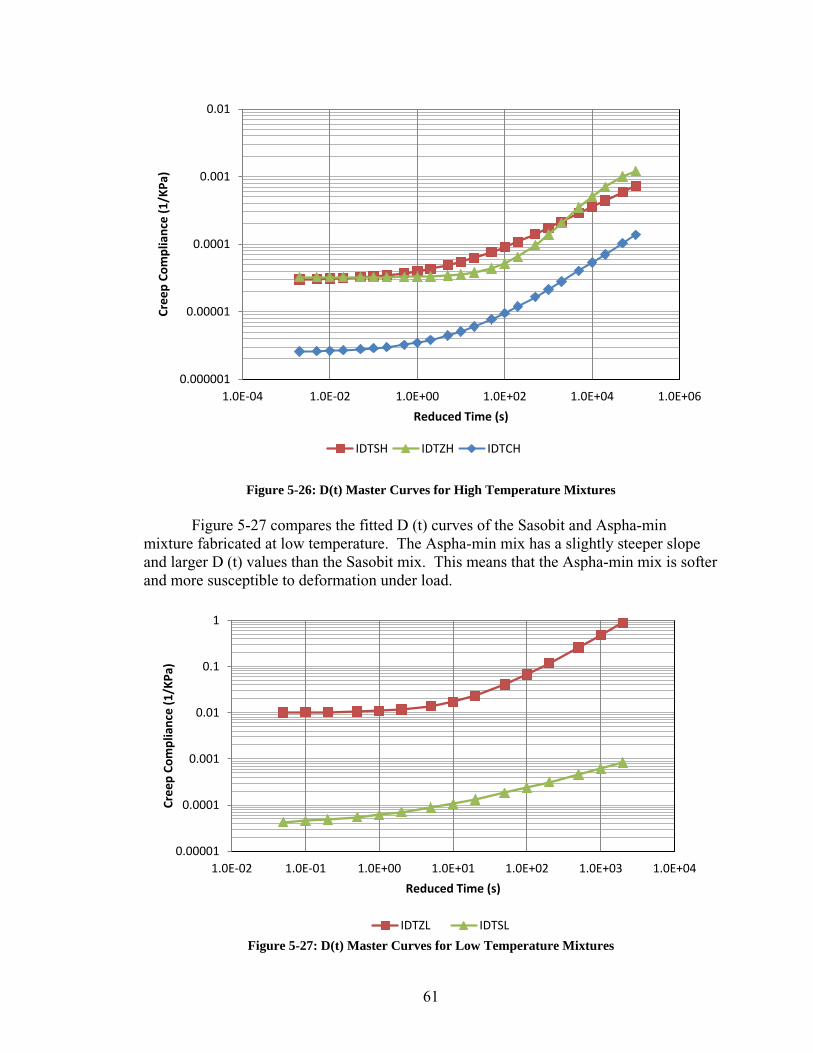
61
Figure 5-26: D(t) Master Curves for High Temperature Mixtures
Figure 5-27 compares the fitted D (t) curves of the Sasobit and Aspha-min
mixture fabricated at low temperature. The Aspha-min mix has a slightly steeper slope and larger D (t) values than the Sasobit mix. This means that the Aspha-min mix is softer and more susceptible to deformation under load.
Figure 5-27: D(t) Master Curves for Low Temperature Mixtures
0.000001
0.00001
0.0001
0.001
0.01
1.0E-04 1.0E-02 1.0E+00 1.0E+02 1.0E+04 1.0E+06
Cre
ep
Co
mp
lian
ce (
1/K
Pa)
Reduced Time (s)
IDTSH IDTZH IDTCH
0.00001
0.0001
0.001
0.01
0.1
1
1.0E-02 1.0E-01 1.0E+00 1.0E+01 1.0E+02 1.0E+03 1.0E+04
Cre
ep
Co
mp
lian
ce (
1/K
Pa)
Reduced Time (s)
IDTZL IDTSL
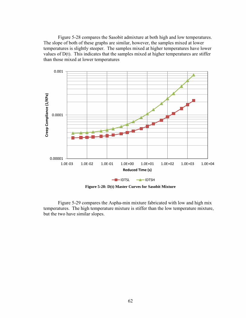
62
Figure 5-28 compares the Sasobit admixture at both high and low temperatures.
The slope of both of these graphs are similar, however, the samples mixed at lower temperatures is slightly steeper. The samples mixed at higher temperatures have lower values of D(t). This indicates that the samples mixed at higher temperatures are stiffer than those mixed at lower temperatures
Figure 5-28: D(t) Master Curves for Sasobit Mixture
Figure 5-29 compares the Aspha-min mixture fabricated with low and high mix temperatures. The high temperature mixture is stiffer than the low temperature mixture, but the two have similar slopes.
0.00001
0.0001
0.001
1.0E-03 1.0E-02 1.0E-01 1.0E+00 1.0E+01 1.0E+02 1.0E+03 1.0E+04
Cre
ep
Co
mp
lian
ce (
1/K
Pa)
Reduced Time (s)
IDTSL IDTSH
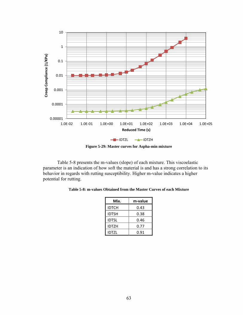
63
Figure 5-29: Master curves for Aspha-min mixture
Table 5-8 presents the m-values (slope) of each mixture. This viscoelastic parameter is an indication of how soft the material is and has a strong correlation to its behavior in regards with rutting susceptibility. Higher m-value indicates a higher potential for rutting.
Table 5-8: m-values Obtained from the Master Curves of each Mixture
Mix. m-value
IDTCH 0.43
IDTSH 0.38
IDTSL 0.46
IDTZH 0.77
IDTZL 0.91
0.00001
0.0001
0.001
0.01
0.1
1
10
1.0E-02 1.0E-01 1.0E+00 1.0E+01 1.0E+02 1.0E+03 1.0E+04 1.0E+05
Cre
ep
Co
mp
lian
ce (
1/K
Pa)
Reduced Time (s)
IDTZL IDTZH

64
5.7 - Thermal stress restrained specimen test (TSRST)
Specimens for TSRST were compacted in the SGC and cut and cored to final dimensions of 150 mm height and 75 mm in diameter. The specimens were glued to the metal platens using 24h epoxy glue one day prior to testing. The thermocouples were attached to the specimens’ surface using modeling clay, which provides adherence and
insulate the thermocouples from the temperature fluctuations inside the chamber. The specimens were left in the chamber for 6 hours at an initial temperature of -5oC to assure an even temperature distribution. The environmental chamber controller was programmed to drop the temperature at a constant rate of 10oC per hour. Due to a shortage of material, TSRST was performed on 12 specimens only. Table 5-9 presents the summary of the results for all the specimens tested.
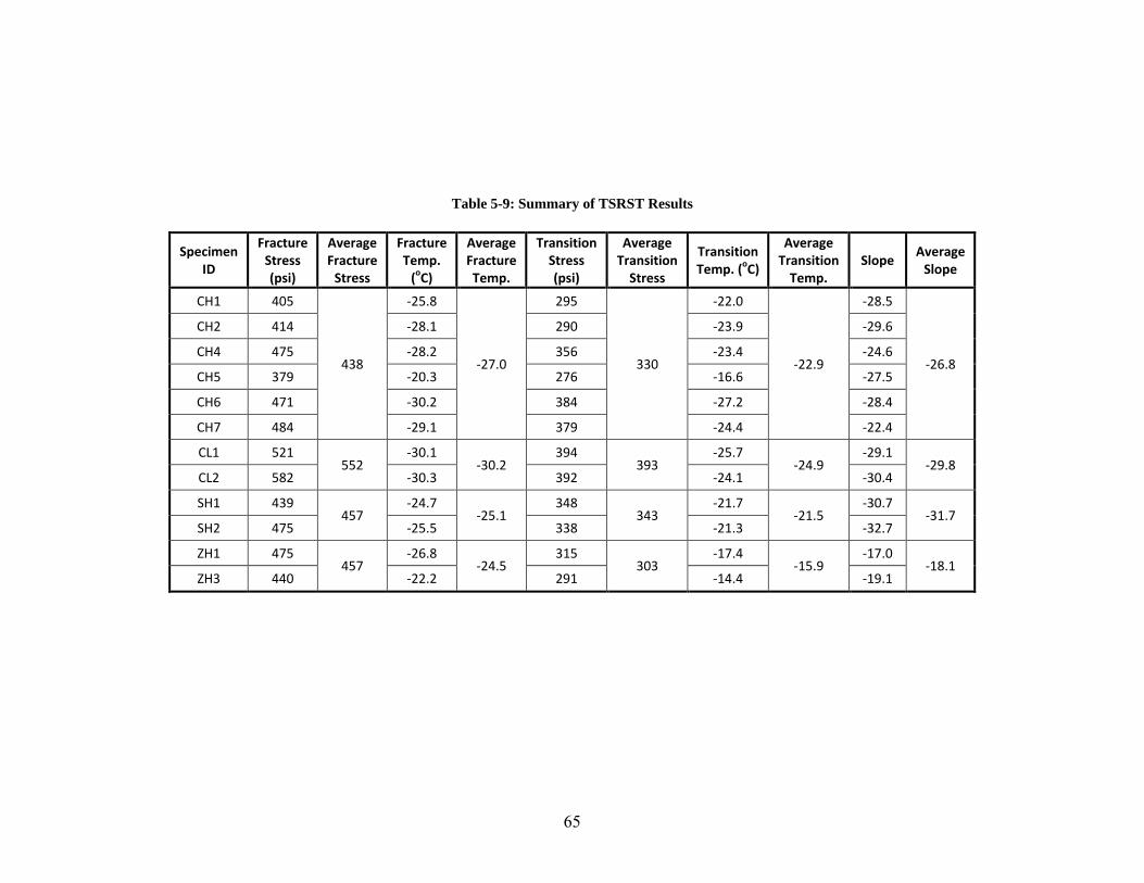
65
Table 5-9: Summary of TSRST Results
Specimen ID
Fracture Stress (psi)
Average Fracture
Stress
Fracture Temp.
(oC)
Average Fracture Temp.
Transition Stress (psi)
Average Transition
Stress
Transition Temp. (oC)
Average Transition
Temp. Slope
Average Slope
CH1 405
438
-25.8
-27.0
295
330
-22.0
-22.9
-28.5
-26.8
CH2 414 -28.1 290 -23.9 -29.6
CH4 475 -28.2 356 -23.4 -24.6
CH5 379 -20.3 276 -16.6 -27.5
CH6 471 -30.2 384 -27.2 -28.4
CH7 484 -29.1 379 -24.4 -22.4
CL1 521 552
-30.1 -30.2
394 393
-25.7 -24.9
-29.1 -29.8
CL2 582 -30.3 392 -24.1 -30.4
SH1 439 457
-24.7 -25.1
348 343
-21.7 -21.5
-30.7 -31.7
SH2 475 -25.5 338 -21.3 -32.7
ZH1 475 457
-26.8 -24.5
315 303
-17.4 -15.9
-17.0 -18.1
ZH3 440 -22.2 291 -14.4 -19.1
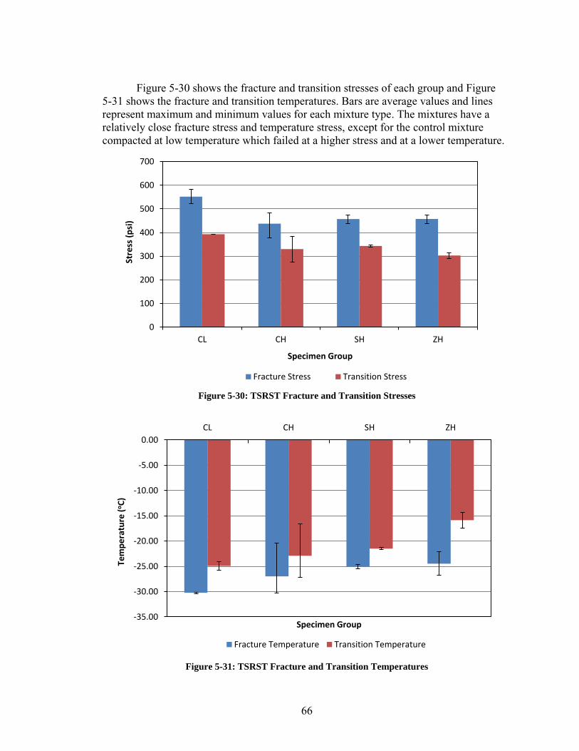
66
Figure 5-30 shows the fracture and transition stresses of each group and Figure
5-31 shows the fracture and transition temperatures. Bars are average values and lines represent maximum and minimum values for each mixture type. The mixtures have a relatively close fracture stress and temperature stress, except for the control mixture compacted at low temperature which failed at a higher stress and at a lower temperature.
Figure 5-30: TSRST Fracture and Transition Stresses
Figure 5-31: TSRST Fracture and Transition Temperatures
0
100
200
300
400
500
600
700
CL CH SH ZH
Stre
ss (
psi
)
Specimen Group
Fracture Stress Transition Stress
-35.00
-30.00
-25.00
-20.00
-15.00
-10.00
-5.00
0.00
CL CH SH ZH
Tem
pe
ratu
re (
oC
)
Specimen Group
Fracture Temperature Transition Temperature
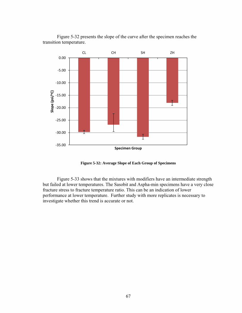
67
Figure 5-32 presents the slope of the curve after the specimen reaches the
transition temperature.
Figure 5-32: Average Slope of Each Group of Specimens
Figure 5-33 shows that the mixtures with modifiers have an intermediate strength but failed at lower temperatures. The Sasobit and Aspha-min specimens have a very close fracture stress to fracture temperature ratio. This can be an indication of lower performance at lower temperature. Further study with more replicates is necessary to investigate whether this trend is accurate or not.
-35.00
-30.00
-25.00
-20.00
-15.00
-10.00
-5.00
0.00
CL CH SH ZHSl
op
e (
psi
/oC
)
Specimen Group
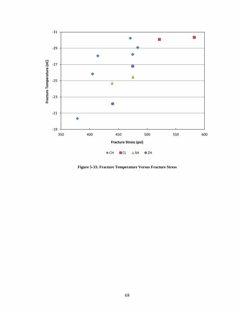
68
Figure 5-33: Fracture Temperature Versus Fracture Stress
-31
-29
-27
-25
-23
-21
-19
350 400 450 500 550 600
Frac
ture
Te
mp
era
ture
(o
C)
Fracture Stress (psi)
CH CL SH ZH

69
5.8 - Results Summary
In this section a summary of the results is presented graphically. The results were divided into four groups: the field mixes ranked according to rutting performance (Figure 5-34), the lab fabricated specimens ranked according to rutting performance (Figure 5-35) and the lab fabricated specimens ranked according to thermal cracking performance (Figure 5-37) and moisture susceptibility (Figure 5-36 and Figure 5-38). This approach makes it possible to evaluate the effects of the mixture’s overall moisture susceptibility
and low temperature performance in a qualitative way. The ranking procedure for rutting performance of the MMLS3 tested specimens
consisted in sorting the results according to the average amount of rutting for each mix. The mix that had the lowest rut depth was ranked first. Only accumulated rut depths after 2000 cycles were taken into account because that was when the measurements became steady and consistent. The creep stiffness from lab fabricated specimens was also used to assess the potential rut resistance.
The m-value was used to rank the mixtures with respect to creep compliance. Larger m-values indicate greater susceptibility to rutting. The IDT results were ranked from highest to lowest TSR value. Thermal cracking performance was ranked using the fracture strength and fracture temperature.
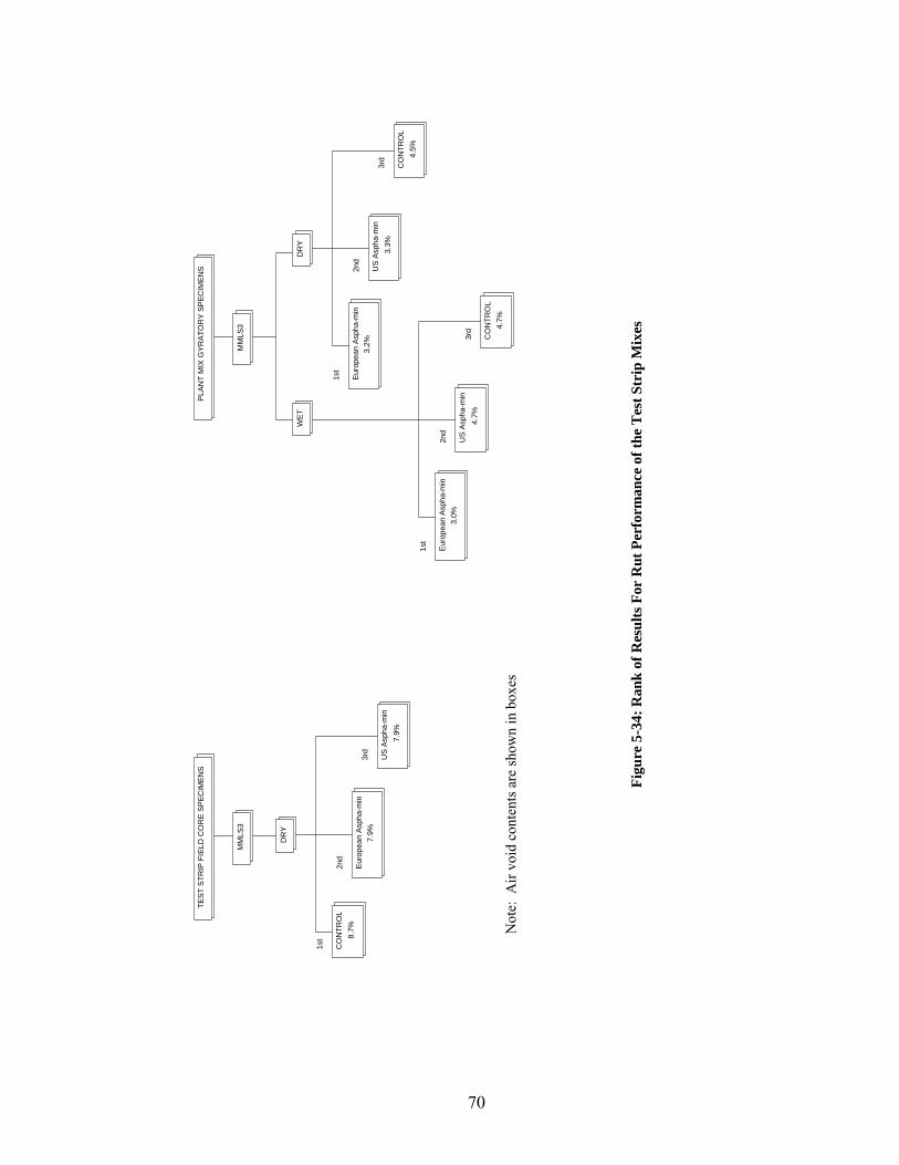
70
MM
LS
3
TE
ST
ST
RIP
FIE
LD
CO
RE
SP
EC
IME
NS
DR
Y
Euro
pea
n A
sph
a-m
in
US
Asph
a-m
in
CO
NT
RO
L
8.7
%
7.9
%
7.9
%
DR
YW
ET
PL
AN
T M
IX G
YR
AT
OR
Y S
PE
CIM
EN
S
Euro
pea
n A
sph
a-m
in
US
Asph
a-m
in
CO
NT
RO
L
4.7
%
3.0
%
4.7
%
3.3
%
3.2
%
4.5
%
CO
NT
RO
L
US
Asph
a-m
in
Euro
pea
n A
sph
a-m
in
1st
2nd
3rd
1st
2nd
3rd
2nd
1st
3rd
MM
LS
3
Fig
ure
5-3
4:
Ra
nk
of
Res
ult
s F
or
Ru
t P
erfo
rma
nce
of
the
Tes
t S
trip
Mix
es
Not
e: A
ir v
oid
cont
ents
are
sho
wn
in b
oxes
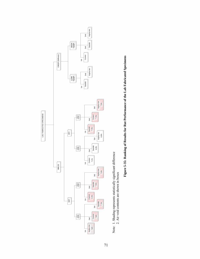
71
CR
EE
P (
Stiffness)
MM
LS
3
LA
B. F
AB
RIC
AT
ED
SP
EC
IME
NS
HIG
HT
EM
P.
TE
MP
.L
OW
WE
TD
RY
LO
WT
EM
P.
TE
MP
.H
IGH
3rd
2nd
1st
7.3
%
Asph
a-m
in
Saso
bit
7.0
%
7.2
%
Con
trol
Saso
bit
7.0
%
6.3
%
Con
trol
Asph
a-m
in
7.6
%
1st
2nd
3rd
3rd
2nd
1st
6.9
%
Asph
a-m
in
Con
trol
7.1
%
6.9
%
Saso
bit
N/A
Asph
a-m
in
7.1
%
3rd
2nd
1st
Con
trol
N/A
Saso
bit
Asph
a-m
inS
aso
bit
Con
trol
1st
2nd
2nd
TE
MP
.LO
WH
IGH
TE
MP
.
2nd
1st Saso
bit
Asph
a-m
in
Fig
ure
5-3
5:
Ra
nk
ing
of
Res
ult
s fo
r R
ut
Per
form
an
ce o
f th
e L
ab
Fa
bri
cate
d S
pec
imen
s
Not
e: 1
. Sha
ding
rep
rese
nts
stat
istic
ally
sig
nifi
cant
dif
fere
nce
2
. Air
voi
d co
nten
ts a
re s
how
n in
box
es
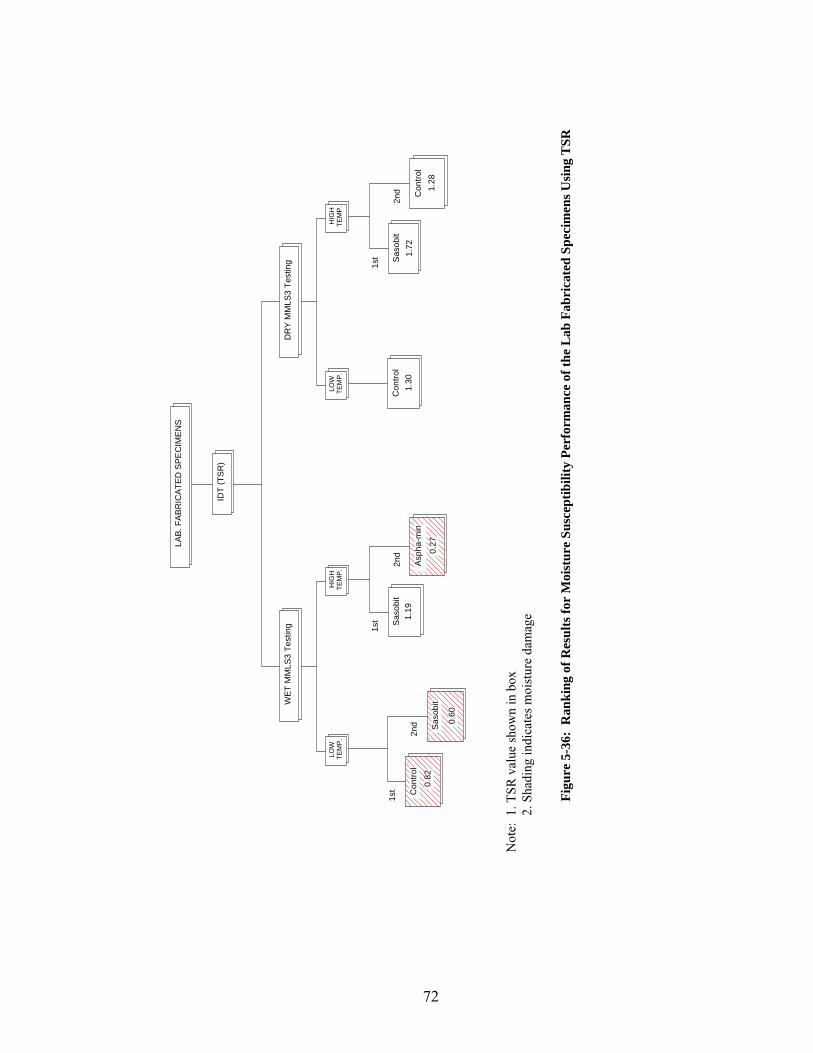
72
Sa
so
bit
Con
tro
l
1st
2n
d
Con
tro
l2
nd
1st
Asp
ha
-min
Sa
so
bit
Con
tro
l
Sa
so
bit
1st
2n
d
HIG
HT
EM
P.
TE
MP
.L
OW
WE
T M
ML
S3
Te
stin
g
LO
WT
EM
P.
TE
MP
.H
IGH
IDT
(T
SR
)
DR
Y M
ML
S3
Te
stin
g
LA
B.
FA
BR
ICA
TE
D S
PE
CIM
EN
S
0.8
2
0.6
0
1.1
9
0.2
7
1.3
0
1.2
8
1.7
2
Fig
ure
5-3
6:
Ran
kin
g o
f R
esu
lts
for
Mo
istu
re S
usc
epti
bil
ity
Per
form
an
ce o
f th
e L
ab
Fa
bri
cate
d S
pec
imen
s U
sin
g T
SR
Not
e: 1
. TSR
val
ue s
how
n in
box
2. S
hadi
ng in
dica
tes
moi
stur
e da
mag
e
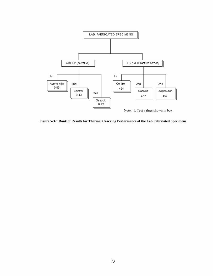
73
Figure 5-37: Rank of Results for Thermal Cracking Performance of the Lab Fabricated Specimens
Note: 1. Test values shown in box
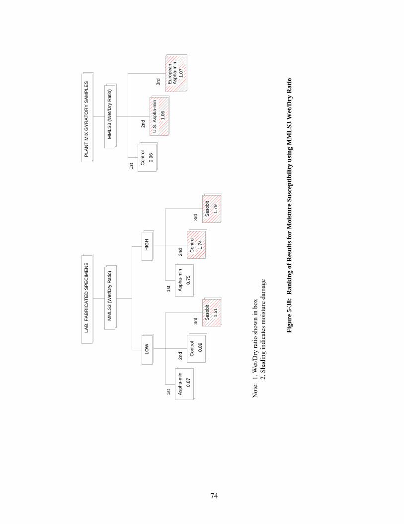
74
LA
B.
FA
BR
ICA
TE
D S
PE
CIM
EN
S
LO
W
Sa
so
bit
0.8
9
Co
ntr
ol
1st
2n
d
3rd
1.5
1
Asp
ha
-min
0.8
7
1st
3rd
2n
d
0.7
5
Asp
ha
-min
Sa
so
bit
1.7
9
1.7
4
Co
ntr
ol
HIG
H
MM
LS
3 (
We
t/D
ry R
atio)
MM
LS
3 (
We
t/D
ry R
atio)
Co
ntr
ol
0.9
6 U
.S. A
sp
ha
-min
1.0
6
2n
d
3rd
1st
PL
AN
T M
IX G
YR
AT
OR
Y S
AM
PLE
S Euro
pean
1.0
7
Asp
ha
-min
Fig
ure
5-3
8:
Ran
kin
g o
f R
esu
lts
for
Mo
istu
re S
usc
epti
bil
ity
usi
ng
MM
LS
3 W
et/D
ry R
ati
o
Not
e: 1
. Wet
/Dry
rat
io s
how
n in
box
2. S
hadi
ng in
dica
tes
moi
stur
e da
mag
e
75
CHAPTER 6
CONCLUSIONS
This report presents the results of a study conducted to evaluate the moisture and
low temperature cracking susceptibility of warm asphalt mixtures made using Aspha-min and Sasobit additives. Evaluation of moisture susceptibility was accomplished by testing lab specimens, available cores, and field sections under accelerated loading (MMLS3) in wet and dry conditions. Low temperature cracking was evaluated through creep compliance and TSRST tests. A secondary goal of this research was to assess whether any difference exists between the American and European versions of the Aspha-min. The conclusions drawn from this study are listed below according to each type of distress:
Rutting
- European Aspha-min exhibited better performance than the US Aspha-min in
the field tests, however the difference is not statistically significant.
- No difference in performance between WMA and HMA was observed from lab specimen results
- Control specimens had the highest modulus for the high mixing temperature
and the Sasobit specimens had the highest modulus for the low mixing temperature. These two mixtures would be expected to have more resistance to rutting in the field than the other mixtures when subjected to the same environmental, structural and loading conditions. However very few specimens were tested and no statistical analysis could be performed
Thermal Cracking
- The results show that the warm mixture additives decrease the thermal cracking performance. More replicate specimens need to be tested in order to verify this behavior.

76
Moisture Susceptibility
- Wet/Dry Rut ratios from MMLS3 testing indicate that Aspha-min mixtures are more susceptible to moisture damage as compared to control specimens, although TSR results from the same specimens didn’t show the same trend.
- The Sasobit mixtures did not exhibit moisture susceptibility. The overall analysis of the data showed that mixtures fabricated with Aspha-min have potential for moisture susceptibility and both Aspha-min and Sasobit have potential for thermal cracking when compared to the control mixture. Future Work Some topics are listed below as recommendation for further study :
- Study of plant mix material. This would make it possible to investigate the effects of the plant production on the performance of the warm mixtures
- Additional testing with more replicates in order to verify the trends observed in this study specially in regards with low temperature testing
- Field section evaluation
77
REFERENCES 1. D’Angelo, John, et al. “Warm-Mix Asphalt: European Practice”. FHWA Report
No. PL-08-007, Federal Highway Administration, US Department of Transportation, February 2008.
2. Newcomb, David. “An Introduction to Warm-Mix Asphalt”. National Asphalt
Paving Association, August 2007. Website: http://fs1.hotmix.org/mbc/ Introduction_to_Warm_Mix_Asphalt.pdf
3. Kristjansdottir, Olof. “Warm Mix Asphalt for Cold Weather Paving”. M.S.
Thesis, University of Washington, 2006. 4. Western Research Institute. “Fundamental Properties of Asphalts and Modified
Asphalts, III”. Report prepared for Federal Highway Administration under Contract No. DTFH61-07-D-00005, December 2007.
5. Hurley, Graham C., and B.D. Prowell. “Evaluation of Aspha-Min Zeolite For Use
In Warm Mix Asphalt”. NCAT Report No. 05-04, National Center for Asphalt Technology, June 2005.
6. Hurley, Graham C., and B.D. Prowell. “Evaluation of Sasobit For Use In Warm
Mix Asphalt”. NCAT Report No. 05-06, National Center for Asphalt Technology, June 2005.
7. Roberts, Freddy L. et al. “Hot Mix Asphalt, Materials, Mixture Design, and
Construction”. National Asphalt Pavement Association Research and Education Foundation, Lanham, MD. 2nd Edition, 1996.
8. Kandhal, Prithvi S. “Moisture Susceptibility of HMA Mixes: Identification of
Problem and Recommended Solutions”. NCAT Report No. 92-1, National Center for Asphalt Technology, May 1992.
9. Corrigan, Matthew. “Warm Mix Asphalt Technologies and Research”. Federal
Highway Administration, October 2008. Website: http://www.fhwa.dot.gov/ pavement/asphalt/wma.cfm
10. Prowell, Brian D. “Warm Mix Asphalt Scan Summary Report”. Federal Highway
Administration – The International Technology Scanning Program, July 2007. 11. “Superpave Mix Design (SP-2)”. Asphalt Institute Executive Offices and
Research Center, Lexington, KY. 3rd Edition, 2001. 12. Mogawer, Walaa S., A.J. Austerman, and M. Turo. “Massachusetts Laboratory
and Field Evaluation of Warm Mix Asphalt”. University of Massachusetts
Dartmouth, July 2006.
78
13. MLS Test Systems. “MMLS3 Traffic Simulator Operator’s Manual”. MLS Test
Systems, April 2002. 14. MLS Test Systems. “MMLS3 Wet Pavement Heater Preliminary Users Manual”.
MLS Test Systems, June 2002. 15. Smit, André de Fortier and F. Hugo. “The Model Mobile Load Simulator as a
Tool for Evaluating Asphalt Performance Under Wet Conditions”. Proceedings of
the 9th International Conference on Asphalt Pavements, Copenhagen, Denmark, August 2002.
16. Smit, André de Fortier et al. “Model Mobile Load Simulator Testing at National
Center for Asphalt Technology Test Track”. Transportation Research Record No.
1832, Paper No. 03-4179, Transportation Research Board, Washington, D.C., 2003
17. MLS Test Systems. “MLS Test Systems P900 Profilometer Operator’s Manual”.
MLS Test Systems, April 2002. 18. Singh, Abhijeet. “Adjustment of Rutting Profiles Obtained Through MMLS3 &
Relation Between Densification Indices and Bailey Parameters”. Research
Internship Report, University of New Hampshire, July 2007. 19. Hugo, Fred et al. “Distress of Hot Mix Asphalt on the NCAT Test Track Due to
Accelerated Wet Trafficking with the MMLS3”. Proceedings of the 2nd
International APT Conference, Minneapolis, MN, 2004. 20. Huang, Yang H. “Pavement Analysis and Design”. Pearson Prentice Hall, Upper
Saddle River, NJ. 2nd Edition, 2004. 21. MLS Test Systems (Pty) Ltd. - Development and Production of Pavement Testing
Systems. Website: http://academic.sun.ac.za/mls/index.htm 22. Smit, André de Fortier et al. “A Discussion of MMLS3 Performance Testing of
Laboratory Prepared HMA Slabs and Briquettes Compared with Hamburg and APA Wheel Tracking Tests”. Proceedings of the 2
nd International APT Conference, Seattle, WA, 2004.
23. Hugo, Fred, R. de Witt, and A. Helmich. “Application of the MMLS3 as APT
Tool for Evaluating Asphalt Performance on a Highway in Namibia”.
Proceedings of the 8th Conference on Asphalt Pavements for Southern Africa, Sun City, South Africa, September 2004.

79
APPENDICES

80
APPENDIX A BATCHING, MIXING, AND COMPACTION PROCEDURE

81
Batching
Equipment Needed:
1. Flat bottom pans (one for each specimen) 2. Scoop 3. Small metal bowl 4. Balance 5. Aluminum Foil Procedure:
1. Create a batching sheet that lists each sieve size and the mass of aggregate required for one specimen for each respective sieve size. The total aggregate should equal the specimen size you are batching (i.e. 4500 g or 2000 g).
2. Gather all buckets containing the required dried aggregate. 3. Place the small metal bowl on the scale and zero the mass. The metal bowl will be
used to transfer measured aggregate to each individual specimen’s pan. 4. Using the scoop measure out the required mass for one specimen (according to the
batching sheet from step #1) from the first aggregate bucket. 5. Transfer the mass of aggregate from the small metal bowl to the first specimen’s pan.
Repeat for each of the remaining specimens. Repeat the measuring process for each of the remaining aggregate buckets. Pile
each aggregate size in a new pile in the pan so that a pile can be removed easily if a mistake is made.
6. Batch the smaller sized aggregate on top of the larger sizes so that the smaller aggregate, especially the dust, does not stick to the bottom of the pan.
7. Cover each pan with a sheet of aluminum foil to prevent contamination or loss of aggregate dust. Label each pan with specimen number and mass of the batch.
Mixing
Equipment Needed:
1. Oven 2. Metal spoons and spatulas 3. Thermometer or hotplate with temperature probe 4. 5 gallon mixing bucket with blade and mixer 5. Propane torch 6. Balance 7. Paper towels 8. Heat resistant gloves 9. Safety glasses Procedure:
1. Place the pans of batched out aggregate into the oven for at least 4 hours at 15°C above the mixing temperature. Mixing bucket, paddle, spoons, and spatulas can be placed in the oven at the same time as batched aggregate or for at least 2 hours prior to mixing.

82
2. Place the asphalt binder in the oven at 15°C above the mixing temperature for 2 hours. Use a thermometer to monitor the temperature of the binder while in the oven. Alternatively the binder can be placed on a hotplate set to the mixing temperature
after approximately 1-1/2 hours in the oven. 3. Begin mixing when the asphalt binder reaches mixing temperature. 4. Remove the mixing bucket from the oven and place it on the scale, zeroing the mass. 5. Remove a pan of batched aggregate from the oven and remove the aluminum foil
cover. 6. Carefully pour the aggregate into the mixing bucket and crate a small well in the
aggregate with a metal spoon. Place the empty aggregate pan back into the oven. 7. Record the mass of the aggregate.
For mixing with Aspha-min zeolite: After the mass of the aggregate is recorded determine the mass of Aspha-min
required (0.3% by weight of total mix) Zero the scale with aggregate in mixing barrel. Using a small scoop, slowly pour the required amount of Aspha-min directly
into the mixing bucket. Using a spoon, mix the Aspha-min and aggregate before adding the liquid
binder. 8. Calculate the amount of asphalt binder required using the mass of the aggregate
For mixing with Sasobit: The total mass of the asphalt binder in a can should be determined before
heating. Measure the mass of Sasobit to be added to the binder (1.5% weight of asphalt
binder) in a small metal bowl. Add Sasobit to the heated liquid binder and stir thoroughly before adding to
the aggregate. 9. Zero the scale. 10. Remove the liquid asphalt from the oven or hotplate and carefully pour the required
mass of binder into the well in the aggregate. A paper towel can be used to remove any excess binder from the aggregate well.
11. Place the asphalt binder back into the oven or onto the hotplate. 12. Insert the mixing bucket into the mixer. Insert the mixing blade and push it down into
the aggregate/binder until it is fully inserted. 13. Turn on the mixer and allow it to mix the aggregate with the binder.
Use the propane torch to heat the outside of the mixing bucket while the mixer is turned on.
Rotate the mixing blade on its peg to scrape the bottom and sides of the mixing bucket while the mixer is turned on. This prevents the fine aggregate from accumulating in the center of the bucket or on the bucket sides.
Be sure to wear safety glasses while the mixer is turned on. 14. When the aggregate is fully coated with asphalt binder stop heating the sides of the
bucket and turn off the mixer. 15. Remove the empty aggregate pan from the oven and place it on the scale, zeroing the
mass.

83
16. Remove the mixing blade and using a spatula, scrape of any accumulated mixture into the empty pan.
17. Remove the mixing bucket from the mixer and carefully pour the mixture into the pan. Use a metal spoon to scrape out any accumulated mixture and add to the pan.
18. Record the resulting mass of the mixture. 19. Spread the mixture evenly in the pan and cover with aluminum foil. 20. Place the pan into the oven set at compaction temperature for the desired aging
period. 21. Place the mixing bucket, blade, spoons, and spatula back into the oven for the next
specimen. This process is repeated for each additional mixing batch. Be sure that spoons, spatulas, mixing bucket and blade are scraped clean of fine aggregate and binder between batches. Aging
For aging, the asphalt mixture should be spread evenly in flat bottom pans, covered with aluminum foil, and labeled with specimen name. Place the pan into the oven set at the compaction temperature for 2 hours.
Compaction
Equipment Needed:
1. Superpave Gyratory Compactor and PC 2. 150 mm diameter Compaction Mold 3. 150 mm diameter Paper Discs (2 per specimen) 4. Spoon and spatula 5. Fan 6. China marker Procedure:
1. Place the mold, spoon, and spatula into the oven at compaction temperature at least one hour before compaction.
2. Turn on the gyratory compactor and open the accompanying software on the PC. 3. Check that the compaction pressure, angle, and gyration speed are set to the correct
values. 4. Set the compaction height to the desired value. 5. After the aging period, remove the compaction mold from the oven and place one
paper disc into the mold. 6. Remove the aged asphalt mixture from the oven and stir with a spoon. 7. Scoop the mixture into the mold being sure to scrape any fine material stuck on the
bottom of the pan into the mold.

84
8. Use a large spatula to ‘rod’ along the inside of the compaction mold, removing any large air voids from the sides.
9. Spread the mixture to level off the top inside the mold and place a paper disc on top of the mixture.
10. Insert the mold into the gyratory compactor. Lower and lock the mold with the corresponding buttons on the gyratory compactor.
11. Start compaction with the PC program’s ‘start’ button. 12. When compaction is complete remove the mold from the compactor and place in
front of the fan to cool. 13. After 5 to 10 minutes, place the mold onto the gyratory compactor’s extrusion ram.
Flip the extrusion switch and allow the specimen to be pushed from the mold. 14. Remove the top paper disc and label the specimen with it’s ID. Allow the specimen to
cool for an additional 5 minutes. 15. When the specimen is cooled sufficiently, carefully remove the specimen from the
ram, remove the bottom paper disc, and label the bottom with the specimen’s ID. 16. Place the specimen in front of the fan to completely cool. 17. Lower the extrusion ram and place the mold spoon, and spatula back in the oven to
reheat for the next specimen. Repeat this process for each additional aged specimen.

85
APPENDIX B
SUPPLEMENTAL MIX DESIGN DATA
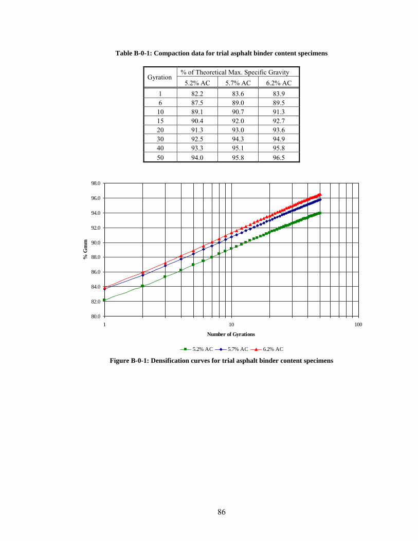
86
Table B-0-1: Compaction data for trial asphalt binder content specimens
Gyration % of Theoretical Max. Specific Gravity
5.2% AC 5.7% AC 6.2% AC
1 82.2 83.6 83.9 6 87.5 89.0 89.5
10 89.1 90.7 91.3 15 90.4 92.0 92.7 20 91.3 93.0 93.6 30 92.5 94.3 94.9 40 93.3 95.1 95.8 50 94.0 95.8 96.5
Figure B-0-1: Densification curves for trial asphalt binder content specimens
80.0
82.0
84.0
86.0
88.0
90.0
92.0
94.0
96.0
98.0
1 10 100
Number of Gyrations
% G
mm
5.2% AC 5.7% AC 6.2% AC
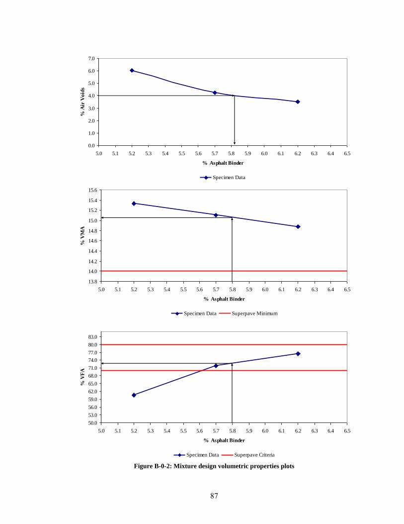
87
Figure B-0-2: Mixture design volumetric properties plots
0.0
1.0
2.0
3.0
4.0
5.0
6.0
7.0
5.0 5.1 5.2 5.3 5.4 5.5 5.6 5.7 5.8 5.9 6.0 6.1 6.2 6.3 6.4 6.5
% Asphalt Binder
% A
ir V
oid
s
Specimen Data
13.8
14.0
14.2
14.4
14.6
14.8
15.0
15.2
15.4
15.6
5.0 5.1 5.2 5.3 5.4 5.5 5.6 5.7 5.8 5.9 6.0 6.1 6.2 6.3 6.4 6.5
% Asphalt Binder
% V
MA
Specimen Data Superpave Minimum
50.0
53.0
56.0
59.0
62.0
65.0
68.0
71.0
74.0
77.0
80.0
83.0
5.0 5.1 5.2 5.3 5.4 5.5 5.6 5.7 5.8 5.9 6.0 6.1 6.2 6.3 6.4 6.5
% Asphalt Binder
% V
FA
Specimen Data Superpave Criteria
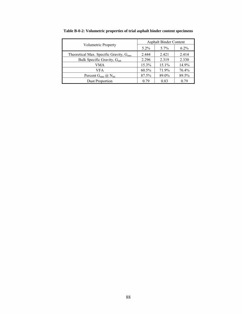
88
Table B-0-2: Volumetric properties of trial asphalt binder content specimens
Volumetric Property Asphalt Binder Content
5.2% 5.7% 6.2%
Theoretical Max. Specific Gravity, Gmm 2.444 2.421 2.414 Bulk Specific Gravity, Gmb 2.296 2.319 2.330
VMA 15.3% 15.1% 14.9% VFA 60.5% 71.9% 76.4%
Percent Gmm @ Nini 87.5% 89.0% 89.5% Dust Proportion 0.79 0.83 0.79
89
APPENDIX C
TEST STRIP FIELD CORE CUMULATIVE DEFORMATION CURVES
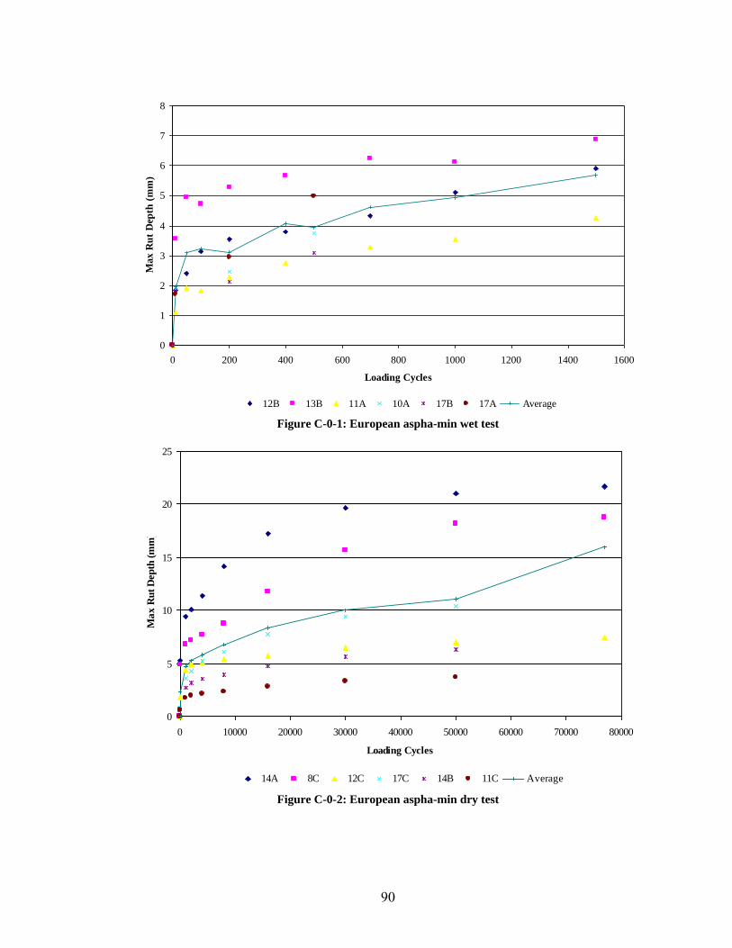
90
Figure C-0-1: European aspha-min wet test
Figure C-0-2: European aspha-min dry test
0
1
2
3
4
5
6
7
8
0 200 400 600 800 1000 1200 1400 1600
Loading Cycles
Max
Ru
t D
epth
(m
m)
12B 13B 11A 10A 17B 17A Average
0
5
10
15
20
25
0 10000 20000 30000 40000 50000 60000 70000 80000
Loading Cycles
Ma
x R
ut
Dep
th (
mm
)
14A 8C 12C 17C 14B 11C Average
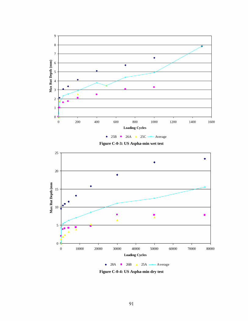
91
Figure C-0-3: US Aspha-min wet test
Figure C-0-4: US Aspha-min dry test
0
1
2
3
4
5
6
7
8
9
0 200 400 600 800 1000 1200 1400 1600
Loading Cycles
Max
Ru
t D
epth
(m
m)
25B 26A 25C Average
0
5
10
15
20
25
0 10000 20000 30000 40000 50000 60000 70000 80000
Loading Cycles
Ma
x R
ut
Dep
th (
mm
)
28A 26B 25A Average
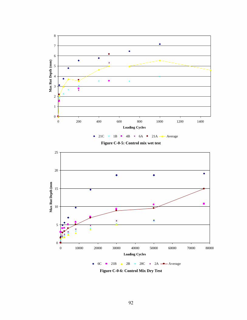
92
Figure C-0-5: Control mix wet test
Figure C-0-6: Control Mix Dry Test
0
1
2
3
4
5
6
7
8
0 200 400 600 800 1000 1200 1400
Loading Cycles
Max
Ru
t D
epth
(m
m)
21C 1B 4B 6A 21A Average
0
5
10
15
20
25
0 10000 20000 30000 40000 50000 60000 70000 80000
Loading Cycles
Ma
x R
ut
Dep
th (
mm
)
6C 21B 2B 20C 2A Average
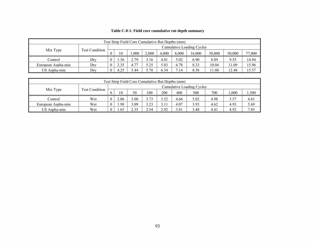
93
Table C-0-1: Field core cumulative rut depth summary
Test Strip Field Core Cumulative Rut Depths (mm)
Mix Type Test Condition Cumulative Loading Cycles
0 10 1,000 2,000 4,000 8,000 16,000 30,000 50,000 77,000
Control Dry 0 1.36 2.79 3.16 4.01 5.02 6.90 8.89 9.55 14.94 European Aspha-min Dry 0 2.35 4.77 5.25 5.83 6.78 8.33 10.04 11.09 15.96
US Aspha-min Dry 0 4.25 5.44 5.78 6.34 7.14 8.58 11.08 12.48 15.57
Test Strip Field Core Cumulative Rut Depths (mm)
Mix Type Test Condition Cumulative Loading Cycles
0 10 50 100 200 400 500 700 1,000 1,500
Control Wet 0 2.06 3.00 3.73 3.52 4.66 5.02 4.98 5.57 4.61 European Aspha-min Wet 0 1.98 3.09 3.23 3.11 4.07 3.93 4.62 4.93 5.69
US Aspha-min Wet 0 1.65 2.35 2.54 2.92 3.81 3.48 4.41 4.92 7.85
94
APPENDIX D
PLANT MIX GYRATORY SPECIMEN CUMULATIVE DEFORMATION
CURVES
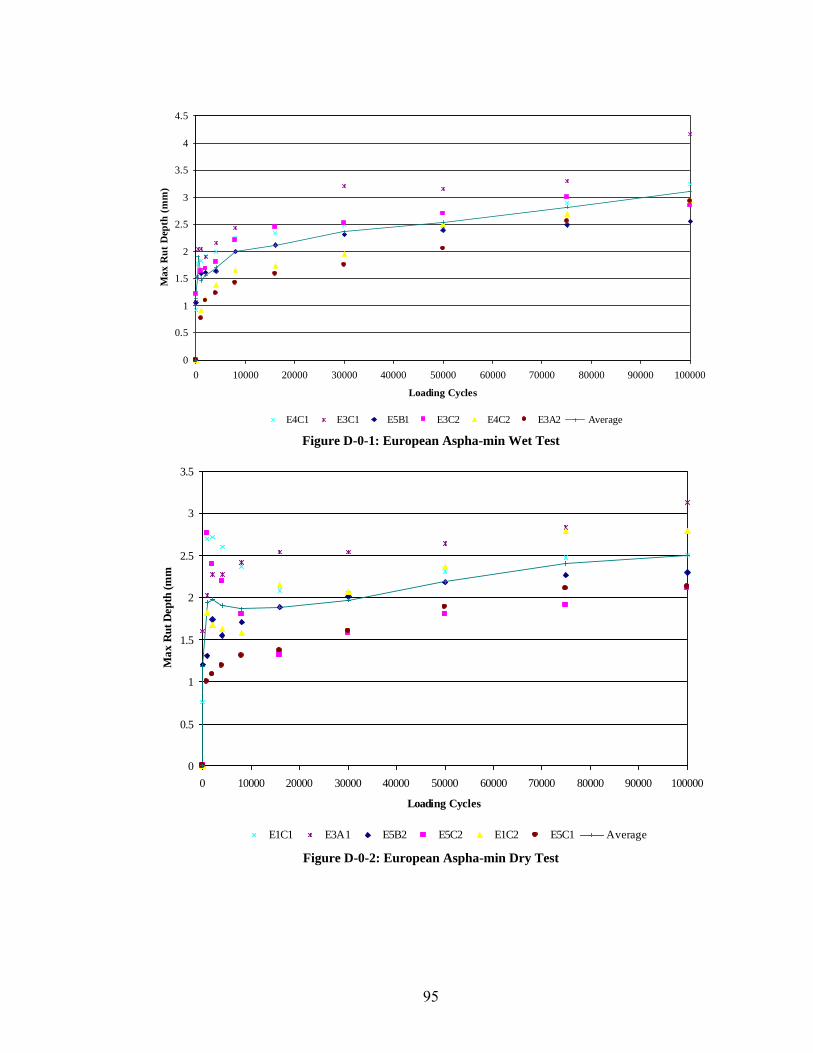
95
Figure D-0-1: European Aspha-min Wet Test
Figure D-0-2: European Aspha-min Dry Test
0
0.5
1
1.5
2
2.5
3
3.5
4
4.5
0 10000 20000 30000 40000 50000 60000 70000 80000 90000 100000
Loading Cycles
Ma
x R
ut
Dep
th (
mm
)
E4C1 E3C1 E5B1 E3C2 E4C2 E3A2 Average
0
0.5
1
1.5
2
2.5
3
3.5
0 10000 20000 30000 40000 50000 60000 70000 80000 90000 100000
Loading Cycles
Ma
x R
ut
Dep
th (
mm
)
E1C1 E3A1 E5B2 E5C2 E1C2 E5C1 Average
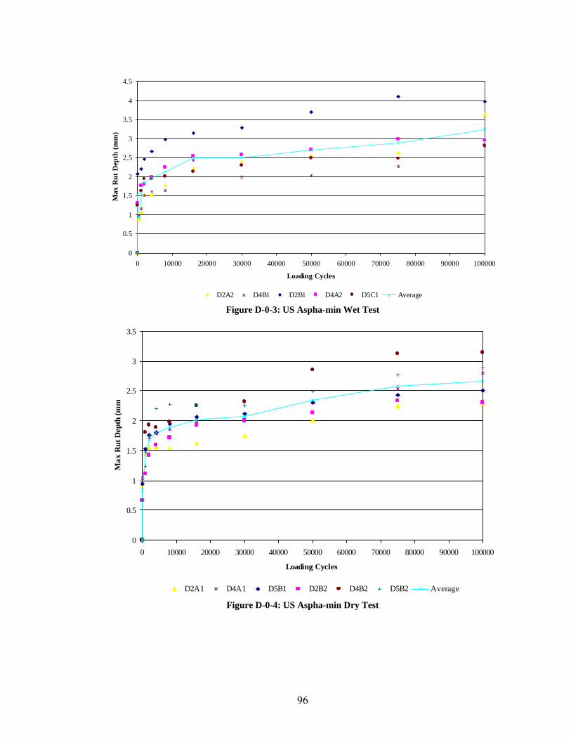
96
Figure D-0-3: US Aspha-min Wet Test
Figure D-0-4: US Aspha-min Dry Test
0
0.5
1
1.5
2
2.5
3
3.5
4
4.5
0 10000 20000 30000 40000 50000 60000 70000 80000 90000 100000
Loading Cycles
Ma
x R
ut
Dep
th (
mm
)
D2A2 D4B1 D2B1 D4A2 D5C1 Average
0
0.5
1
1.5
2
2.5
3
3.5
0 10000 20000 30000 40000 50000 60000 70000 80000 90000 100000
Loading Cycles
Ma
x R
ut
Dep
th (
mm
)
D2A1 D4A1 D5B1 D2B2 D4B2 D5B2 Average
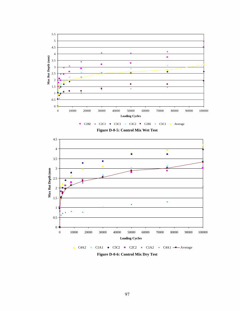
97
Figure D-0-5: Control Mix Wet Test
Figure D-0-6: Control Mix Dry Test
0
0.5
1
1.5
2
2.5
3
3.5
4
4.5
5
5.5
0 10000 20000 30000 40000 50000 60000 70000 80000 90000 100000
Loading Cycles
Ma
x R
ut
Dep
th (
mm
)
C2B2 C2C1 C3C1 C3C2 C2B1 C5C1 Average
0
0.5
1
1.5
2
2.5
3
3.5
4
4.5
0 10000 20000 30000 40000 50000 60000 70000 80000 90000 100000
Loading Cycles
Ma
x R
ut
Dep
th (
mm
)
C4A2 C1A1 C5C2 C2C2 C1A2 C4A1 Average
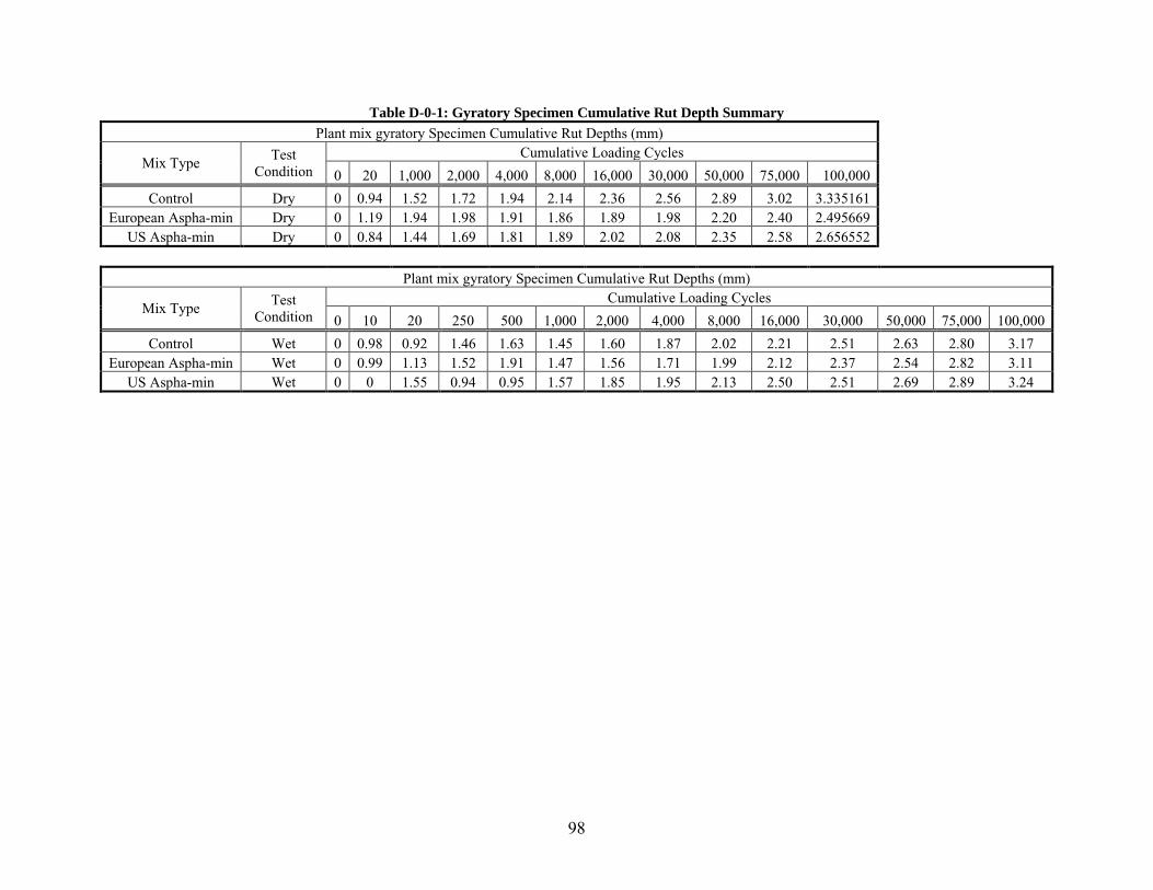
98
Table D-0-1: Gyratory Specimen Cumulative Rut Depth Summary
Plant mix gyratory Specimen Cumulative Rut Depths (mm)
Mix Type Test
Condition Cumulative Loading Cycles
0 20 1,000 2,000 4,000 8,000 16,000 30,000 50,000 75,000 100,000
Control Dry 0 0.94 1.52 1.72 1.94 2.14 2.36 2.56 2.89 3.02 3.335161 European Aspha-min Dry 0 1.19 1.94 1.98 1.91 1.86 1.89 1.98 2.20 2.40 2.495669
US Aspha-min Dry 0 0.84 1.44 1.69 1.81 1.89 2.02 2.08 2.35 2.58 2.656552
Plant mix gyratory Specimen Cumulative Rut Depths (mm)
Mix Type Test
Condition Cumulative Loading Cycles
0 10 20 250 500 1,000 2,000 4,000 8,000 16,000 30,000 50,000 75,000 100,000
Control Wet 0 0.98 0.92 1.46 1.63 1.45 1.60 1.87 2.02 2.21 2.51 2.63 2.80 3.17 European Aspha-min Wet 0 0.99 1.13 1.52 1.91 1.47 1.56 1.71 1.99 2.12 2.37 2.54 2.82 3.11
US Aspha-min Wet 0 0 1.55 0.94 0.95 1.57 1.85 1.95 2.13 2.50 2.51 2.69 2.89 3.24
99
APPENDIX E
LABORATORY FABRICATED SPECIMEN CUMULATIVE
DEFORMATION CURVES
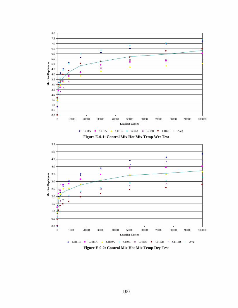
100
Figure E-0-1: Control Mix Hot Mix Temp Wet Test
Figure E-0-2: Control Mix Hot Mix Temp Dry Test
0.0
0.5
1.0
1.5
2.0
2.5
3.0
3.5
4.0
4.5
5.0
5.5
6.0
6.5
7.0
7.5
8.0
0 10000 20000 30000 40000 50000 60000 70000 80000 90000 100000
Loading Cycles
Ma
x R
ut
Dep
th (
mm
)
CH8A CH1A CH1B CH2A CH8B CH6B Avg
0.0
0.5
1.0
1.5
2.0
2.5
3.0
3.5
4.0
4.5
5.0
5.5
0 10000 20000 30000 40000 50000 60000 70000 80000 90000 100000
Loading Cycles
Ma
x R
ut
Dep
th (
mm
)
CH11B CH11A CH10A CH9B CH10B CH12B CH12B Avg
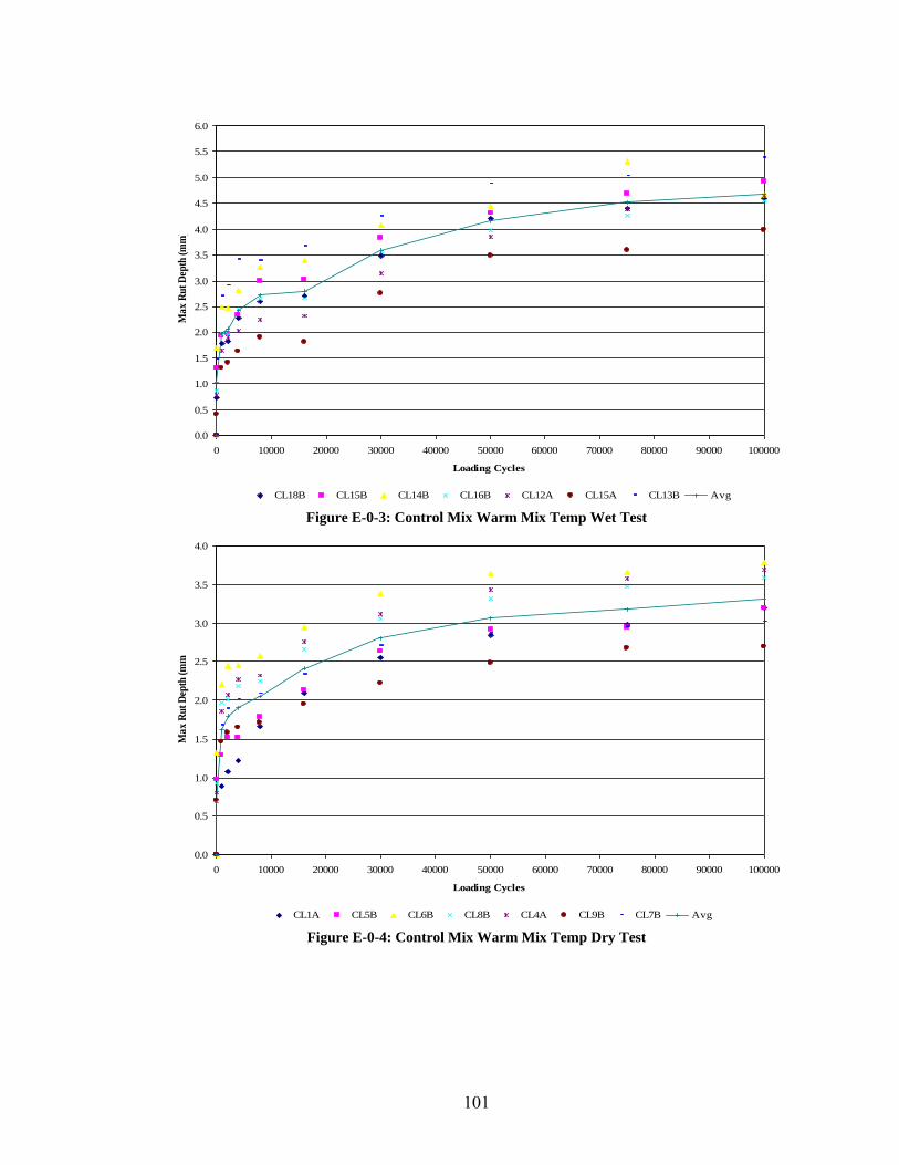
101
Figure E-0-3: Control Mix Warm Mix Temp Wet Test
Figure E-0-4: Control Mix Warm Mix Temp Dry Test
0.0
0.5
1.0
1.5
2.0
2.5
3.0
3.5
4.0
4.5
5.0
5.5
6.0
0 10000 20000 30000 40000 50000 60000 70000 80000 90000 100000
Loading Cycles
Ma
x R
ut
Dep
th (
mm
)
CL18B CL15B CL14B CL16B CL12A CL15A CL13B Avg
0.0
0.5
1.0
1.5
2.0
2.5
3.0
3.5
4.0
0 10000 20000 30000 40000 50000 60000 70000 80000 90000 100000
Loading Cycles
Ma
x R
ut
Dep
th (
mm
)
CL1A CL5B CL6B CL8B CL4A CL9B CL7B Avg
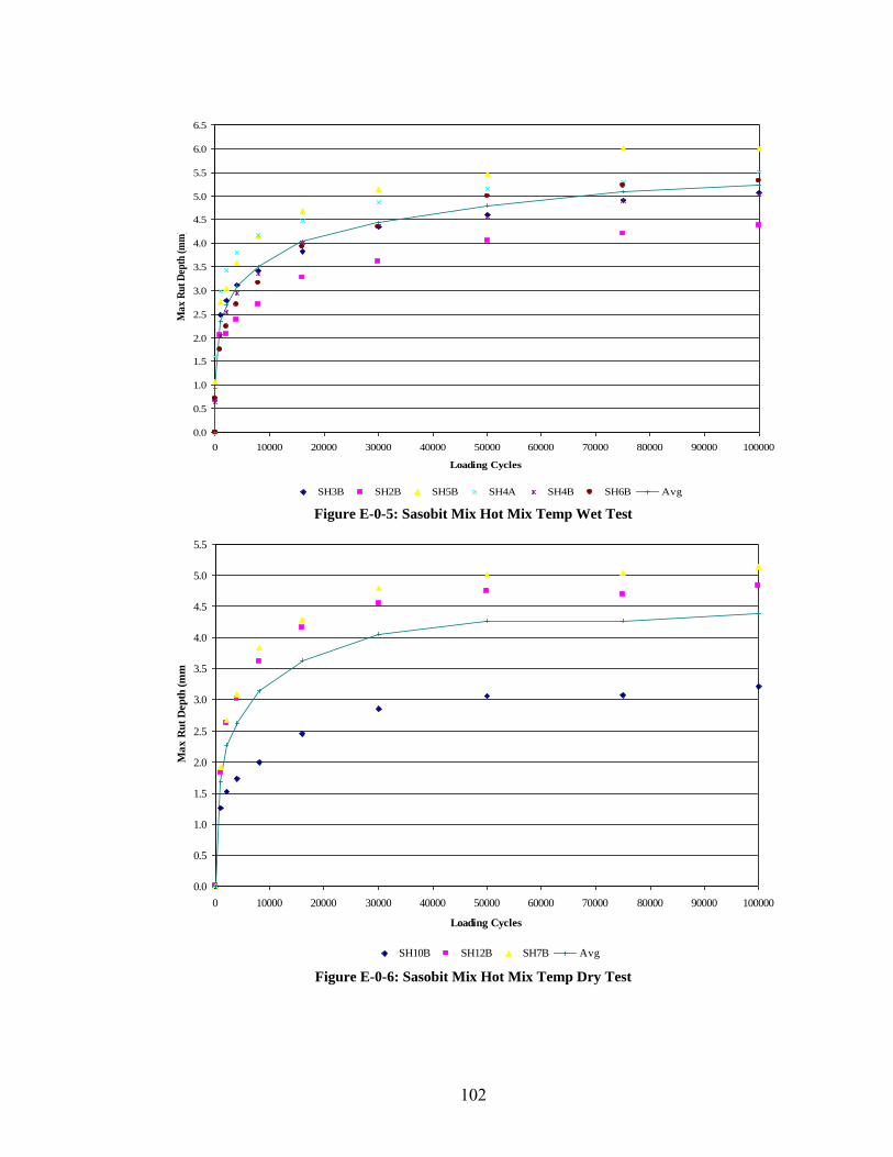
102
Figure E-0-5: Sasobit Mix Hot Mix Temp Wet Test
Figure E-0-6: Sasobit Mix Hot Mix Temp Dry Test
0.0
0.5
1.0
1.5
2.0
2.5
3.0
3.5
4.0
4.5
5.0
5.5
6.0
6.5
0 10000 20000 30000 40000 50000 60000 70000 80000 90000 100000
Loading Cycles
Ma
x R
ut
Dep
th (
mm
)
SH3B SH2B SH5B SH4A SH4B SH6B Avg
0.0
0.5
1.0
1.5
2.0
2.5
3.0
3.5
4.0
4.5
5.0
5.5
0 10000 20000 30000 40000 50000 60000 70000 80000 90000 100000
Loading Cycles
Ma
x R
ut
Dep
th (
mm
)
SH10B SH12B SH7B Avg
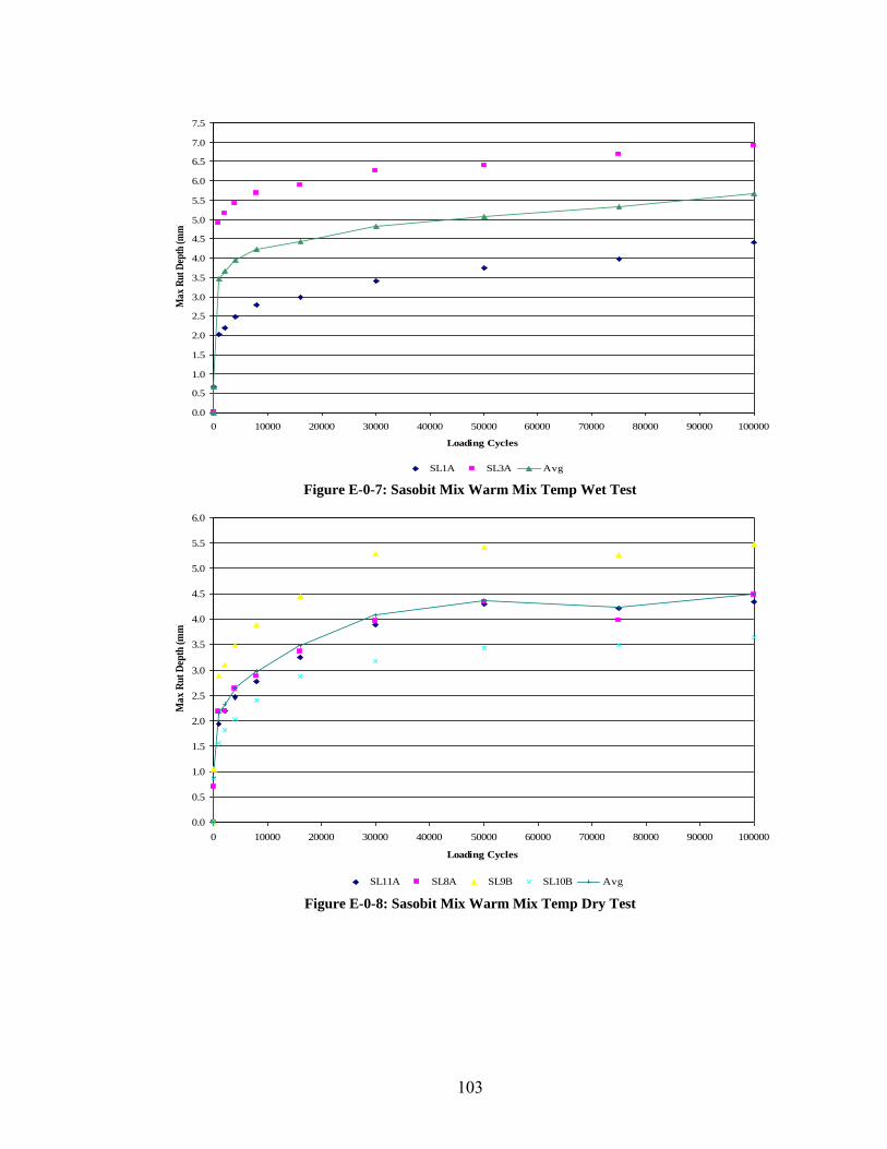
103
Figure E-0-7: Sasobit Mix Warm Mix Temp Wet Test
Figure E-0-8: Sasobit Mix Warm Mix Temp Dry Test
0.0
0.5
1.0
1.5
2.0
2.5
3.0
3.5
4.0
4.5
5.0
5.5
6.0
6.5
7.0
7.5
0 10000 20000 30000 40000 50000 60000 70000 80000 90000 100000
Loading Cycles
Ma
x R
ut
Dep
th (
mm
)
SL1A SL3A Avg
0.0
0.5
1.0
1.5
2.0
2.5
3.0
3.5
4.0
4.5
5.0
5.5
6.0
0 10000 20000 30000 40000 50000 60000 70000 80000 90000 100000
Loading Cycles
Ma
x R
ut
Dep
th (
mm
)
SL11A SL8A SL9B SL10B Avg
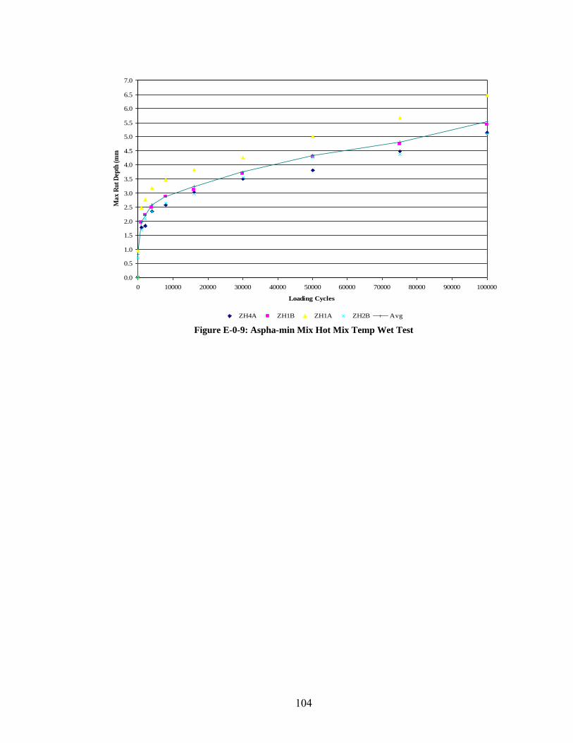
104
Figure E-0-9: Aspha-min Mix Hot Mix Temp Wet Test
0.0
0.5
1.0
1.5
2.0
2.5
3.0
3.5
4.0
4.5
5.0
5.5
6.0
6.5
7.0
0 10000 20000 30000 40000 50000 60000 70000 80000 90000 100000
Loading Cycles
Ma
x R
ut
Dep
th (
mm
)
ZH4A ZH1B ZH1A ZH2B Avg
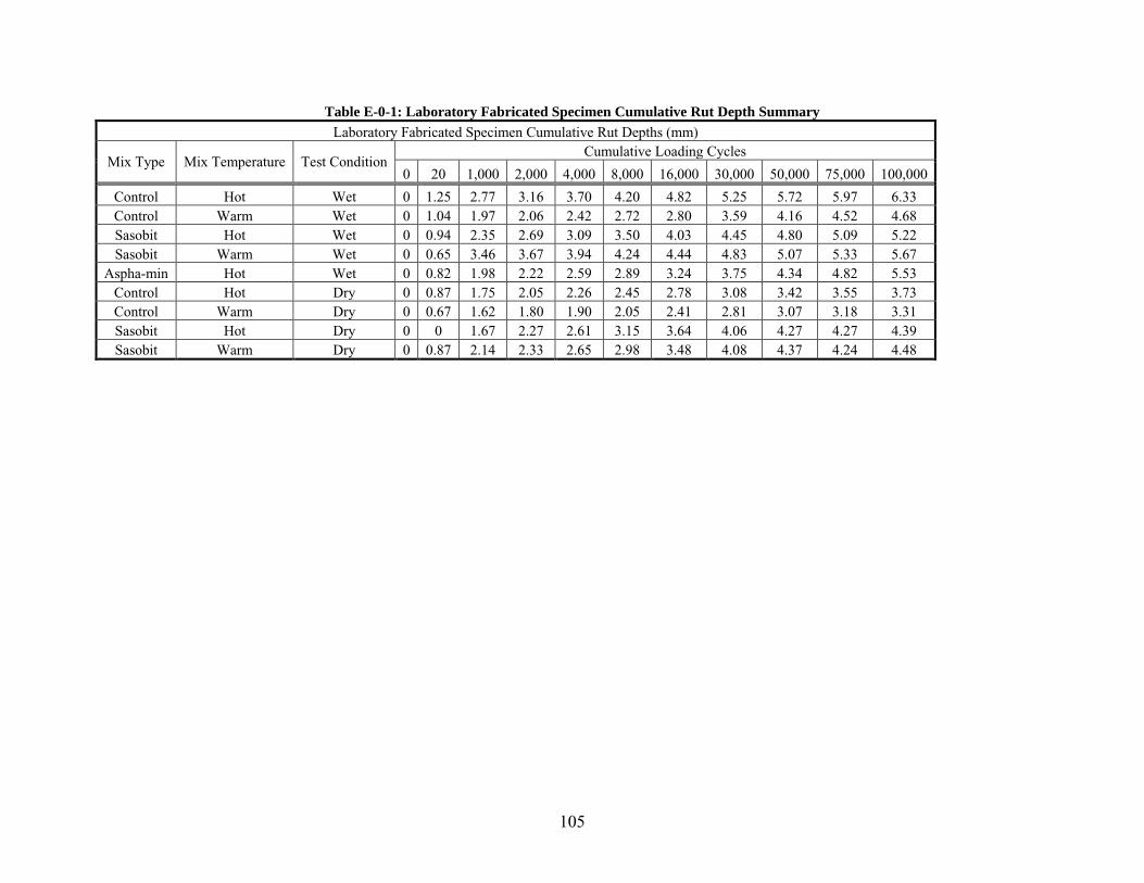
105
Table E-0-1: Laboratory Fabricated Specimen Cumulative Rut Depth Summary
Laboratory Fabricated Specimen Cumulative Rut Depths (mm)
Mix Type Mix Temperature Test Condition Cumulative Loading Cycles
0 20 1,000 2,000 4,000 8,000 16,000 30,000 50,000 75,000 100,000
Control Hot Wet 0 1.25 2.77 3.16 3.70 4.20 4.82 5.25 5.72 5.97 6.33 Control Warm Wet 0 1.04 1.97 2.06 2.42 2.72 2.80 3.59 4.16 4.52 4.68 Sasobit Hot Wet 0 0.94 2.35 2.69 3.09 3.50 4.03 4.45 4.80 5.09 5.22 Sasobit Warm Wet 0 0.65 3.46 3.67 3.94 4.24 4.44 4.83 5.07 5.33 5.67
Aspha-min Hot Wet 0 0.82 1.98 2.22 2.59 2.89 3.24 3.75 4.34 4.82 5.53 Control Hot Dry 0 0.87 1.75 2.05 2.26 2.45 2.78 3.08 3.42 3.55 3.73 Control Warm Dry 0 0.67 1.62 1.80 1.90 2.05 2.41 2.81 3.07 3.18 3.31 Sasobit Hot Dry 0 0 1.67 2.27 2.61 3.15 3.64 4.06 4.27 4.27 4.39 Sasobit Warm Dry 0 0.87 2.14 2.33 2.65 2.98 3.48 4.08 4.37 4.24 4.48