Technical Report Documentation Page 1. Report No.

SWUTC/09/476660-00015-1

2. Government Accession No.

3. Recipient's Catalog No.

4. Title and Subtitle

SUSTAINABLE INTERSECTION CONTROL TO ACCOMMODATE URBAN FREIGHT MOBILITY

5. Report Date

August, 2009 6. Performing Organization Code

7. Author(s)

Bruce X. Wang and Kai Yin 8. Performing Organization Report No.

9. Performing Organization Name and Address

Texas Transportation Institute Texas A&M University System College Station, Texas 77843-3135

10. Work Unit No. (TRAIS)

11. Contract or Grant No.

DTRT07-G-0006 12. Sponsoring Agency Name and Address

Southwest Region University Transportation Center Texas Transportation Institute Texas A&M University System College Station, Texas 77843-3135

13. Type of Report and Period Covered

Technical Report Sep. 2008 – Aug. 2009 14. Sponsoring Agency Code

15. Supplementary Notes

Supported by a Grant From the U.S. Department of Transportation, University Transportation Centers Program

16. Abstract

In this research, we studied green extension of a two-phased vehicle−actuated signal at an isolated intersection between two one-way streets. The green phase is extended by a preset time interval, referred to as critical gap, from the time of a vehicle arrival. The green phase switches if there is no arrival during the critical gap. We developed a model following a Poisson process that studied the intersection performance of traffic. We extended the model to cover the case of general traffic. Additionally, we derived system performance measures. Our findings show that our model is fairly flexible in accommodating freight traffic, and our model in the general case is asymptotically accurate under heavy traffic. Numerical tests show that the presence of critical gaps increases vehicle delay in most cases. This finding is enlightening regarding current practices.

17. Key Words

Intersection Control; Signal Timing; Actuated Signal System

18. Distribution Statement

No restrictions. This document is available to the public through NTIS: National Technical Information Service Springfield, Virginia 22161 http://www.ntis.gov

19. Security Classif.(of this report)

Unclassified

20. Security Classif.(of this page)

Unclassified 21. No. of Pages

54

22. Price

Form DOT F 1700.7 (8-72)

Reproduction of completed page authorized

Sustainable Intersection Control

Accommodating Urban Freight Mobility

by

Bruce X. Wang and Kai Yin Department of Civil Engineering

Texas A&M University

Research Report SWUTC/09/476660-00015-1

August 2009

TEXAS TRANSPORTATION INSTITUTE Texas A&M University System

College Station, Texas 77843-3135

v

ABSTRACT

In this report, we studied green extension of a two-phased vehicle actuated signal at an isolated

intersection between two one-way streets. The green phase is extended by a preset time interval,

referred to as critical gap, from the time of a vehicle arrival. The green phase switches if there is

no arrival during the critical gap. We developed a model following a Poisson process that studied

the intersection performance of traffic. We extended the model to the case of general traffic.

Additionally, we derived the system performance measures. Our findings show that our model is

flexible in accommodating freight traffic and that our model in the general case is asymptotically

accurate under heavy traffic. Numerical tests show that presence of critical gaps increases

vehicle delay in most cases. This finding is enlightening regarding current practices.

vi

vii

EXECUTIVE SUMMARY Traffic engineers always believe that appropriate design of signals can effectively improve the

urban mobility for both passenger and commercial vehicles. However, the complexity in signal

control and traffic behavior often makes it difficult to understand the effects of control policies.

Although many theoretical papers have conducted analyses of signal control strategies, a clear

view on how critical factors determine signal efficiency is still lacking. The objectives of this

study are to systematically examine the performance of a popular vehicle-actuated signal control.

We chose to study an intersection between two one-way streets. We hope through this special

case to gain insights into the properties of general actuated signal systems.

This study was sponsored by the Southwest Regional University Transportation Center

(SWUTC) at Texas A&M University from September 1, 2008, through August 31, 2009. Dr.

Bruce Wang was the principal investigator of this research. Some of the results herein are from

Dr. Wang’s research prior to this project.

In this research, we studied a particular operational strategy for the actuated signal system. An

advance detector is located at a certain distance prior to an intersection such that an arriving

vehicle triggers a green time extension after the queue has been discharged. The extended green

period actuated by the vehicle is called critical gap in this report. If there is no vehicle actuation

during the critical gap, the green phase switches to clear queues in other approaches. In this way,

the actuated system dynamically allocates green time according to vehicle arrivals from multiple

approaches. The control strategy therefore reduces to determining the green extension.

Vehicle waiting time at an intersection is a critical performance measure of intersection control.

Because of the uncertainty of traffic arrivals, the average waiting time for vehicles is used. The

average waiting time is a function of several signal and intersection characteristics, such as the

expectation and the variance of green time, which themselves also serve as performance

measures. In considering environmental impact, the number of stop-and-goes is used as an

alternative performance measure as opposed to the average waiting time. Developing stochastic

viii

models is necessary for the performance because of their capability of accommodating the

stochastic traffic.

The optimal solution is developed for the case in which traffic follows Poisson arrival processes.

However, when the traffic follows a general stochastic process, such as a general renewal

process, an approximated method is needed for performance analysis. Therefore, approximated

solutions have been developed for the case of general but heavy traffic. In the case of heavy

traffic, the results are asymptotically optimal.

We have found in almost all cases that the optimal control is to switch the signal as soon as the

queue had been cleared in one direction. This strategy leads to minimized average vehicle

waiting time, regardless of consideration of environmental emissions, with both homogeneous

and heterogeneous traffic. The research team believes that this finding can be generalized to the

actuated signal system with more than two approaches. In practice, detection of queue existence

could adopt various technologies. If vehicle headway is used for this purpose, it would be

impossible to reduce the critical gap to zero. In this case, the critical gap is set to an appropriate

small value. This practical convenience, however, takes a toll on the system performance in most

cases, according to our findings in this research.

ix

TABLE OF CONTENTS

Page List of Illustrations ........................................................................................................................ x

Figures ......................................................................................................................................... x

Tables........................................................................................................................................... x

Disclaimer ...................................................................................................................................... xi

Acknowledgments ....................................................................................................................... xii

Chapter 1: Introduction ................................................................................................................ 1

Background .................................................................................................................................. 1

Objective of This Study ............................................................................................................... 3

Chapter 2: Expectation and Variance of Green Times .............................................................. 5

Problem Statement ....................................................................................................................... 5

Expected Green Times ................................................................................................................. 8

Variance of Green Times ........................................................................................................... 11

Symmetric Intersections ............................................................................................................ 16

Chapter 3: Vehicle Delay ............................................................................................................ 19

Vehicle Delay for a Single Cycle .............................................................................................. 19

Vehicle Delay Per Unit Time .................................................................................................... 21

Environmental Concerns ........................................................................................................... 24

Optimal Control to Accommodate Commercial Vehicle Movement ........................................ 25

Chapter 4: General Vehicle Headway Under Heavy Traffic .................................................. 27

Chapter 5: Discussion and Conclusion ...................................................................................... 32

References ..................................................................................................................................... 35

Appendix....................................................................................................................................... 37

A. Derivation .......................................................................................................................... 37

B. Figures ............................................................................................................................... 39

x

LIST OF ILLUSTRATIONS

FIGURES

Page

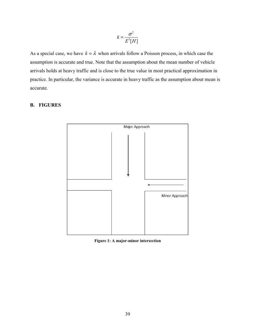
Figure 1: A major-minor intersection ............................................................................................ 39

Figure 2: An illustrative queueing process in minor approach ...................................................... 40

Figure 3: Example average delay per unit time with 2.0δ = , 0.15sλ = and 0.25Lλ = ............... 40

Figure 4: Example average delay per unit time with 4.0δ = , 0.02sλ = and 0.25Lλ = ................ 41

Figure 5: Realizations of cumulative queue .................................................................................. 42

TABLES

Page

Table 1: Optimal critical gap and intersection performance with 2.0δ = .................................... 23

Table 2: Optimal critical gap and intersection performance with 4.0δ = .................................... 23

Table 3: Optimal critical gap and environmental concerns with 2.0δ = ..................................... 25

Table 4: Optimal critical gap and environmental concerns with 4.0δ = ..................................... 25

Table 5: Optimal critical gap and heterogeneous traffic with 2.0δ = .......................................... 26

Table 6: Optimal critical gap and heterogeneous traffic with 4.0δ = .......................................... 26

xi

DISCLAIMER

The contents of this report reflect the views of the authors, who are responsible for the facts and

accuracy of the information presented herein. This document is disseminated under the

sponsorship of the U.S. Department of Transportation, University Transportation Centers

Program in the interest of information exchange. The U.S. Government assumes no liability for

the contents or use thereof.

xii

ACKNOWLEDGMENTS

This project was conducted with support from the U.S. Department of Transportation, University

Transportation Centers Program to the Southwest Regional University Transportation Center.

1

CHAPTER 1: INTRODUCTION

BACKGROUND

Vehicle-actuated signal systems have been widely adopted in traffic control for their adaptability

to traffic arrivals in urban areas. Vehicle mobility, including that of commercial vehicles, and

transportation system sustainability are closely related to design of the control strategies at these

intersections. A number of studies and practical applications have concluded that vehicle-

actuated intersection control promotes sustainability and urban mobility.

Intersection control has several implications. One is reduction of overall vehicle delay at

intersections. This is important for growing urban areas. Second, proper intersection control

helps improve environment protection. Vehicle stop-and-go at intersections causes

environmental concerns, and appropriate intersection control can minimize the number of stop-

and-goes. A third implication is that signal control can adapt to different traffic mixes with

vehicles of differing characteristics, such as varying values of time. For instance, commercial

vehicles’ value of time is significantly different from that of passenger cars. An optimal

intersection control strategy should explicitly consider heterogeneity of traffic mix.

This study concerns the optimal structure of intersection control at vehicle-actuated signals.

Despite the fact that single systems have been used for decades, the optimal structure of the

control policy for a vehicle-actuated intersection has not been clear, especially with

heterogeneous vehicle mixes. We address these challenges in this project.

Historical Evolution

There is a long history of vehicle-actuated signals. The first traffic signals appeared in London in

the United Kingdom in December, 1868. They resembled railway signals of the time. In the

United States, the first electric signals were installed in Cleveland, Ohio, in 1914, for the purpose

of allowing police and fire stations to control the signals in case of an emergency (USPTO,

1913). In 1926, the first vehicle-actuated signal (a horn-actuated signal) was made in the United

2

States by placing microphones on the side of the road. In the 1930s and thereafter, vehicle-

actuated signals were constructed. During the 1950s and 1960s, with the improvement of

engineering techniques, the vehicle-actuated signal system became more and more popular and

attracted the attention of traffic engineering researchers.

Relevant Literature

Research on vehicle-actuated control traces back to the 1940s. Clayton (1941) studied the

average delay at vehicle-actuated signals on a minor road with light traffic. Tanner (1953)

estimated the delays of two opposing streams of vehicles trying to cross a length of road wide

enough for only one vehicle at a time. Based on his assumption, he found explicit results for

waiting times for only some special cases.

Darroch et al. (1964) gave a complete analysis based on assumptions of general distribution of

departure vehicle headways and lost time, and of exponential distributed arrival headways. The

authors used results of standard queueing theory to investigate the influence of green extension

to signal cycle and average delay. In addition, Newell (1969) was primarily concerned with

vehicle-actuated control strategies under the arrival probability invariant to time translations.

This model did not assume any specific probability function for the arrivals but a linear

relationship between the mean and variance of arrivals within any given time period.

Furthermore, he evaluated the mean and variance of the cycle time. An important result is that he

showed that the cycle time had a gamma distribution.

Based on a binomial vehicle arrival, Dunne (1967) presented a discrete model following Darroch

et al. (1964). He gave an analytic expression of the probability generating function for vehicle

delay and showed a connection to the discrete cases of Darroch et al. (1964). Little (1971) also

considered a classic discrete model and obtained probability distribution of queue length in the

steady state.

Taking bunching arrivals into consideration, Cowan (1978) also considered vehicle-actuated

traffic control. The intersection under his consideration was similar to that of Darroch et al.

(1964) in that the intersection was between two one-way streets. The difference between the two

3

was that the latter assumed a vehicle detector upstream of the intersection while Cowan (1978)

assumed it at the stop line of the intersection. He assumed that the bunch of arrivals, separated by

inter-bunch headway of shifted exponential distribution, has a general distribution size and the

intra-bunch gap has a constant one unit time. The control policy he considered is that the green

phase ceases as soon as there is no departure at an allotted time for a particular backward interval

length. Our research here follows the assumption in Cowan (1978).

There are also many other proposed models similar to the ones above. Examples include Morris

and Pak-Poy (1967) and Lin (1982). Recently, Viti and Zuylen (2009) developed a

computational probability model based on an assumption of any temporal distribution of input.

Thus, the temporal evolution of queue length, signal sequence probabilities, delay, and waiting

time can be computed. Their model can serve as a probabilistic evaluation for microscopic

simulations and is also suitable for planning. However, their computational model does not give

theoretical insight to control strategy. Readers cannot obtain an optimal control strategy through

their analysis.

On the practical front, Kruger et al. (1990) studied the real implementation of vehicle-actuated

control at an intersection. They investigated the location of detectors for a specific strategy:

queue control. Queue control strategy aims to detect the end of the queue and switches the signal

at the same time that the end of the queue is expected to reach the intersection. Based on

numerical simulation, they showed that, in general, queue control at an isolated intersection is

better than other control strategies. The queue control strategy corresponds to the case in our

model that the critical gap is zero. We analytically show why queue control is optimal in most

cases.

OBJECTIVES OF THIS STUDY

This study mainly focused on assessment of properties for vehicle-actuated signal timing. In

particular, it had the following objectives.

• Examining the stochastic properties of signal timing in this particularly popular signal

control scheme when vehicle arrivals follow Poisson processes,

4

• Identifying optimal signal control strategies in this actuated signal system,

• Examining the impact of freight mobility on the optimal configuration of signal

control with the concerns of total delays and environmental impact respectively, and

• Examining the stochastic properties of signal timing with a general arrival

distribution under heavy traffic.

Outline of This Report

In this report, we define our problem in Chapter 2. This is followed by a derivation of analytical

formulas for the expected green time, as well as variances. Chapter 3 addresses the average

vehicle delay in terms of expected green time and variance of green time. Also, numerical

solutions and some important implications from the optimal control strategy are presented in this

chapter. Chapter 4 reports the actuated control under general arrival pattern. We conclude this

report in Chapter 5 by summarizing the major results and highlighting some future challenges.

5

CHAPTER 2: EXPECTATION AND VARIANCE OF GREEN TIMES

PROBLEM STATEMENT

Modeling methodologies of actuated intersection control highly depends on configuration of

intersections. Sometimes, a slight difference as small as the presence of left turning lanes can

pose great challenges in model development or its resultant accuracy. Problem setup therefore

appears critical. In choosing an intersection for this study, we have several concerns. First, the

intersection should provide general insights to other intersections. Second, the intersection setup

should be mathematically maneuverable.

In order to guide the subsequent model development, the study problem is defined as follows1.

We consider an actuated signal system at an isolated intersection between two one-way streets

without turning vehicles, denoted by major and minor approaches respectively. We assume that

there are only two green phases, each dedicated to traffic in one approach. Vehicle arrivals from

the two approaches follow two independent, homogeneous Poisson processes. We consider a

special yet popular control scheme that first of all ensures queue clearance during a green phase.

After waiting vehicles are discharged, if there is a vehicle arrival at time t , the green phase is

extended until time t + Δ . Δ is called critical gap. If, however, there is no vehicle arrival during

the green period extended, say, [ , ]t t + Δ , the green phase switches to its conflict approach

automatically, resulting in a loss of effective green time. The critical gaps are denoted by sΔ and

LΔ for the minor and major approaches, respectively. In each approach, there is a constant

discharge rate to clear waiting vehicles. Obviously, the critical gaps sΔ and LΔ are the only

control variables. The objective is to decide the values of sΔ and LΔ such that the average vehicle

delay at the intersection over a long period is minimized.

1 Similar setups are also seen in Darroch et al. (1964), Newell (1969), and Cowan (1978).

6

It is clear that the critical gap is the only control variable in this control scheme. Figure 1 in

Appendix B illustrates such an intersection. For the ease of understanding, we assume that there

is only one lane in each direction.

Note that in this idealized study problem, we do not consider the physical location of the loop

detector. We assume that it is determined by the critical gap, or that it is simply located at the

intersection. We further assume that there is no minimum green time in each approach, as we

assume that there is an available technology to detect the vehicle queue presence. The queue

clearance time is therefore assumed known to the system each time. Each time after dissipating

the queue, the preset critical gap is applied. This setup allows us to study for the full potential in

efficient signal control. In addition, we do not consider the physical sizes of the roadway, the

intersection, or the vehicles, which is consistent to the point queue model. For the purpose of

presentation, we only consider homogeneous passenger cars in the model. In a later section, we

will discuss impact and strategies of commercial vehicles.

Strategy

For simplicity, we assume a strategy in which the green phase always switches to its conflict

approach when there is no vehicle arrival during the period of a critical gap.

We refer to this strategy as the always-switch strategy. This strategy is also assumed in Darroch

et al. (1964). Although the always-switch strategy could give rise to a `peculiar' situation in

which the green phase switches to the minor approach without any waiting vehicles, and then

switches back to the major approach, there is a high probability of vehicle presence at the time of

switch. Therefore, we have reasonable confidence that the analysis under this strategy makes a

good approximation to the actual performance.

The always-switch strategy could also have practical representations. For example, a mobile

server travels between two different locations to serve customers in two different geographic

areas. Each time the machine moves, some effective service time is lost. If there is no

communication between the two service sites, we have an always-switch strategy.

7

As will be seen, vehicle delay and green times are functions of the total green time loss during a

signal cycle, irrespective of its split between the two switches. For simplicity, we denote the total

green time loss withδ , which, in another word, is the total time loss for the two switches during

one signal cycle.

We present the notation next. Note that the subscripts s and L correspond to minor and major

approaches, respectively.

Notation

sλ vehicle arrival rate along the minor approach

Lλ vehicle arrival rate along the major approach

sΔ critical gap in the minor approach

LΔ critical gap in the major approach

st random green time in the minor approach

Lt random green time in the major approach

sf discharge rate of vehicular queue along the minor approach

Lf discharge rate of vehicular queue along the major approach

δ total green time loss in a signal cycle due to phase switches

[ ]E expected value function

( )Var variance function

( )COV covariance function

( )X random number of arrivals with the parameter being time period.

The parameters of the intersection, such as the green time loss and queue discharge rates, are all

considered deterministic in this report. We believe that assuming randomness for them would

only increase technical complexity slightly and that it would not dramatically change the nature

of the results. In addition, the critical gaps, once set up, do not change.

8

EXPECTED GREEN TIMES

In each approach, the green time consists of two random components: queue clearance time and

free flow time. The queue clearance time represents the period in which the discharging rate of

vehicles equals the saturation rate, denoted by sat and Lat for both approaches, respectively. The

free flow time, denoted by sbt and Lbt for both approaches respectively, corresponds to the period

of time, the length of which is a function of the critical gap and vehicle arrivals. In the free flow

time, there is no presence of vehicular queue. Note that the duration of free flow time is a

function of the critical gap, while the latter is the endogenous variable to be studied. For

instance, if the critical gap is set to be zero, which means the signal switches immediately after

queue clearance, the free flow time turns to be zero.

As studied in Wang (2007), sbt and Lbt are determined by an information relay process:

1 1[ ] s s

sbs s

E t eλ

λ λΔ= − and

1 1[ ] L L

LbL L

E t eλ

λ λΔ= − . To summarize, we have s sa sbt t t= + and

L La Lbt t t= + . Due to the Markov property, sat and sbt are independent of each other. The same is

true for sbt and Lbt . In Appendix B, Figure 2 shows an illustrative queueing process in the minor

direction during a cycle. Next, we show how to evaluate sat . Since the discharge rate of vehicles

at the intersection remains constant, then sat should be a multiple of sf . However, for convenient

analysis, we can still use the continuous model to evaluate the stochastic properties. Doing this

would not make the results different. Therefore, sat satisfies the following relationship for traffic

flow conservation.

( ) ( ) 0L sa s saX t X t f tδ+ + − = (1)

where ( )X represents the number of arrivals in a Poisson process along the minor approach.

Equation (1) states that the total number of vehicles discharged at the saturation rate in time sat

equals the total arrivals during L sat tδ+ + . Equation (1) ensures a full discharge rate during sat .

9

Taking expectation at both sides of Equation (1) gives the following expected queue clearance

time. It is worthy to note that sat is a function of arrival distribution and departure rate; thus any

attempt to take expectation or variance by conditioning on sat and Lt will lead to incorrect results.

Here we can replace sat and Lt by their expectation first and then take expectation at both sides of

Equation (1). In the next section, another method using queueing theory will be provided.

[ ]

[ ] s L ssa

s s

E tE t

f

λ λ δλ+=

−

Similarly,

[ ][ ] L s L

LaL L

E tE t

f

λ λ δλ+=

−

Therefore, we have

[ ] [ ] [ ]

[ ] 1 1s s

s sa sb

s L s

s s s s

E t E t E t

E te

fλλ λ δ

λ λ λΔ

= ++= + −

− (2)

In the same way,

[ ] [ ] [ ]

[ ] 1 1L L

L La Lb

L s L

L L L L

E t E t E t

E te

fλλ λ δ

λ λ λΔ

= ++= + −

− (3)

Solving Equations (2) and (3) gives [ ]sE t and [ ]LE t as follows.

Proposition 1. The expected lengths of green phases are given as follows.

( )( ) 1 1[ ]

1 1

s s

s L

L L

s s L L ss

L s L s s s s s

s L

s s L L L L

f fE t e

f f f f f

ef f

λ

λ

λ λ λ δλ λ λ λ λ

λ λ δλ λ λ λ

Δ

Δ

− −= × + −− − −

+ + − − −

(4a)

10

and

( )( ) 1 1[ ]

1 1

L L

s L

s s

s s L L LL

L s L s L L L L

sL

L L s s s s

f fE t e

f f f f f

ef f

λ

λ

λ λ λ δλ λ λ λ λ

λ δλλ λ λ λ

Δ

Δ

− −= × + −− − −

+ + − − −

(4b)

From Proposition 1, it is clear that green duration in each approach is a function of the critical

gaps and all other characteristics (such as discharge rate, arrival rate, and green loss) in both

approaches. This demonstrates the dynamics between both approaches. As 1s L

s Lf f

λ λ+ → , the

expected green times in both approaches become infinite. This is clear by making a change to the

denominator in the first term: (1 )s L

s LL s L s L s

s L

f f f f f ff f

λ λλ λ− − = − − .

The effect of the green lossδ becomes clearer when we set the critical gaps to zero. In this case,

Equations (4a) and (4b) become the following.

[ ]s L

s Ls

L s L s

fE t

f f f f

λ δλ λ

=− −

(5a)

and

[ ]s L

L sL

L s L s

fE t

f f f f

λ δλ λ

=− −

(5b)

We can easily have the following result.

[ ]

[ ]s s L

L L s

E t f

E t f

λλ

=

Specially, the ratio of green times is proportionate to the ratio of vehicle arrival intensities if the

discharge rates are equal in both approaches.

11

Then in this case, the expected duration of a full signal cycle becomes as follows.

[ ] [ ]

1

s L

s L

s L

C E t E t

f f

δδ

λ λ

= + +

=− −

(6)

It is clear from above that the expected cycle length is proportionate to the green loss and that it

increases with the intersection saturation rate: s L

s Lf f

λ λ+ .

The following result summarizes the above discussion.

Corollary 1. When the critical gaps are set to zero, the ratio between the expected green

duration and the cycle length in both approaches is proportionate to s

sf

λ and L

Lf

λ, respectively.

The expected cycle length is 1 s L

s Lf f

δλ λ− −

.

The above property mimics that from the preset timing system with uniform vehicle arrivals.

VARIANCE OF GREEN TIMES

One objective of this study is to investigate the stochastic properties of the signal system cycle.

For this purpose, we need to evaluate the variances of green phases. Variances of green phases

are an important measure of intersection stability. They are also needed in the calculation of the

average vehicle delay.

Variances in both approaches are inter-related. If the duration of the green phase in one approach

becomes longer, expectedly the duration of the green phase in its conflict approach becomes

longer as well. As a result, if the variance of the green duration in one approach becomes larger,

expectedly the variance in its conflict approach becomes larger as well. The derivation in this

section exploits this observation to establish recursive equations. Note that the following

derivation implies an assumption that there exist stationary variances in both approaches.

12

To evaluate variance of green time, we can resort to the results from standard queueing theory

when the discharge headway follows a general distribution. This will lead to results that are not

transparent. Furthermore, it is still debatable whether or not this makes the model more realistic.

In addition, our observation shows a very stable and constant discharge rate when vehicle queues

are present. Therefore, in this section the vehicle departure headway at an intersection is seen as

constant and this treatment cannot change the results far from reality.

We suppose there is a vehicle at the stop line at the beginning of the green time in the minor

approach. Discharging this vehicle takes a time interval, sH , where 1

ss

Hf

= . During this interval

there might be several vehicles arriving to join the queue, and those vehicles also need to be

discharged. This discharging procedure continues until the queue is cleared. We denote the time

period for this discharging procedure by 1χ and denote its probability distribution function by

( )P x where 1( ) { }P x P xχ= ≤ . If there is a queue containing ivehicles at the beginning of the

green time, we denote the similar period for discharging this queue by iχ and its related

distribution by ( )iP x where ( ) { }i iP x P xχ= ≤ . It is easy to see that ( )iP x is an i-fold convolution

of ( )P x , which is equivalent to cleaning iqueues of only one vehicle each. By the theorem of

total probability, we have the relationship:

10

( ){ } { }

!s s

iHs s

i si

HP x e P x H

iλλχ χ

∞−

=

≤ = ≤ −

To prove this relationship, we only need to note that during the departure period sH of the first

vehicle, the number of arrivals follows Poisson distribution. If we let 1( ) ( )ss E e χ−Γ = , the

Laplace-Stieltjes transform of ( )P x , then from the above analysis we have the following

relationship:

( )

0

0

( )( ) { }

!

( )( ( ))

!

s s i s

s s s

iH s Hs s

i

iH sH is s

i

Hs e E e

i

He e s

i

λ χ

λ

λ

λ

∞− − +

=

∞− −

=

Γ =

= Γ

13

To get this equation we need to note that Laplace-Stieltjes transform of ( )iP x is i-th product of

( )sΓ . Hence we have:

( ) exp{ ( ( ) )}s s ss H s sλ λΓ = Γ − − (7)

Using the derivatives of Equation (7) at the point where 0s = , we can get any moment of 1χ .

Now we can evaluate the random variable sat . Suppose in the minor approach that the red time

Lt and the lost time,δ , are known. During the time interval Lt δ+ , the number of arrivals

follows Poisson distribution. By the theorem of total probability, we have:

( )

0

( ( )){ } { }

!s L

its L

sa ii

tP t x e P x

iλ δλ δ χ

∞− +

=

+≤ = ≤

Forming the Laplace-Stieltjes transform of { }saP t x≤ , denoted by ( )F s , we have the following

equation:

0

( )

00

( ) { }

( ( )){ }

!

exp{ ( )( ( ) 1)}

i L

sxsa

it sxs L

ii

s L

F s e dP t x

te e dP x

i

t s

λ δλ δ χ

λ δ

+∞ −

+∞ +∞− + −

=

= ≤

+= ≤

= + Γ −

(8)

From Equation (7) it is easy to evaluate the first and second derivatives of ( )sΓ at 0s = :

' 1(0)

s sf λΓ = −

− (9a)

''3

(0)( )

s

s s

f

f λΓ =

− (9b)

Hence, the expected sat conditional on Lt δ+ is:

' ( )[ | ] (0) s L

sa Ls s

tE t t F

f

λ δδλ++ = − =

− (10)

This equation agrees with the equation in the previous section if we take expectation of Lt δ+ .

The variance of sat conditional on Lt δ+ can be estimated as:

14

'' ' 2

3

( | ) (0) ( (0))

( )

( )

sa L

s s L

s s

Var t t F F

f t

f

δλ δ

λ

+ = −+=

− (11)

To obtain unconditional variances of sat and Lat , we need to use the relation:

( ) [ ( | )] ( [ | ])sa sa L sa LVar t E Var t t Var E t tδ δ= + + +

By using Equations (10) and (11) we have:

2

3 2

( [ ] )( ) ( )

( ) ( )s s L s

sa Ls s s s

f E tVar t Var t

f f

λ δ λλ λ

+= +− −

(12)

In previous analyses, the green time contains two periods: queue clearance time and free flow

time. Because of the Markov property, these two periods are independent of each other. As a

result, we have:

( ) ( ) ( )s sa sbVar t Var t Var t= +

According to Wang (2007), 2

2 2

21( )

s s s ss

sbs s s

e eVar t

λ λ

λ λ λ

Δ ΔΔ= − − + . Therefore, we have the equations

for variances:

22

3 2 2 2

( [ ] ) 21( ) ( )

( ) ( )

s s s ss s L s s

s Ls s s s s s s

f E t e eVar t Var t

f f

λ λλ δ λλ λ λ λ λ

Δ Δ+ Δ= + − − +− −

(13a)

and similarly,

22

3 2 2 2

( [ ] ) 21( ) ( )

( ) ( )

L L L LL L s L L

L sL L L L L L L

f E t e eVar t Var t

f f

λ λλ δ λλ λ λ λ λ

Δ Δ+ Δ= + − − +− −

(13b)

It is clear now that ( )sVar t and ( )LVar t are linear functions of each other. Solving Equations

(13a) and (13b) gives values of ( )sVar t and ( )LVar t as follows.

15

Proposition 2. The equilibrium solutions for variances of green phases are given as follows.

12 2 2

2 2 3 2

3

( [ ] )( ) 1

( ) ( ) ( ) ( )

( [ ] ) ( ) ( )

( )

s L s s L ss

s s L L s s s s

L L sLb sb

L L

f E tVar t

f f f f

f E tVar t Var t

f

λ λ λ δ λλ λ λ λ

λ δλ

− += − + − − − −

+× + + −

(14a)

12 2 2

2 2 3 2

3

( [ ] )( ) 1

( ) ( ) ( ) ( )

( [ ] ) ( ) ( )

( )

s L L L s LL

s s L L L L L L

s s Lsb Lb

s s

f E tVar t

f f f f

f E tVar t Var t

f

λ λ λ δ λλ λ λ λ

λ δλ

− += − + − − − −

+× + + −

(14b)

where 2

2 2

21( )

s s s ss

sbs s s

e eVar t

λ λ

λ λ λ

Δ ΔΔ= − − + and2

2 2

21( )

L L L LL

LbL L L

e eVar t

λ λ

λ λ λ

Δ ΔΔ= − − + . [ ]sE t and [ ]LE t

are given by Equations (4a) and (4b). It is interesting to evaluate the green phases when the critical gap is set to zero, as indicated in

the optimal solution later. This strategy is in fact the queue control strategy studied by Kruger et

al. (1990). In this case, both ( )saVar t and ( )LaVar t become zero. Equations (14a) and (14b)

become:

2 2( ) ( [ ] ) ( [ ] )( )

( ) ( )

L L s s L s L L ss

s s L L

f f E t f E tVar t C

f f

λ λ δ λ λ δλ λ

− + += + − − (15a)

and

2 2( ) ( [ ] ) ( [ ] )( )

( ) ( )

s s L L s L s s LL

L L s s

f f E t f E tVar t C

f f

λ λ δ λ λ δλ λ

− + += + − − (15b)

where

16

2 2

1

1 1 2s sL Ls L s s L L

s L s L

C

f f f ff f f f

λ λλ λ λ λ=

− − − − +

(16)

With Equations (15a) and (15b), we can examine the impact of saturation rate on variances and

intersection stability. Now we take a look at the constant C , represented as Equation (16) at the

right-hand sides of both Equations (15a) and (15b).

It is easily seen by Equations (5a) and (5b) that as ( LVar t , the expected green times increase at a

rate of 1

1 s L

s L

Of f

λ λ−

− −

. But the variances shown by Equations (15a) and (15b) approach

infinity much faster, at a rate of 1

1 s L

s L

Of f

λ λ−

− −

. This means that as the traffic flow reaches

the capacity of an intersection, the system quickly becomes instable. Combined with Equations

(5a) and (5b), Equations (15a) and (15b) imply the following result.

Proposition 3. Given an actuated intersection with zero critical gap, both the expected values

and variances of the green times increase in a linear manner with the total green time lossδ .

The above result indicates the critical role of green time loss in the performance of an

intersection.

SYMMETRIC INTERSECTIONS

In particular, if the two approaches are symmetric, we have s Lλ λ λ= = and s Lf f f= = . The

following result becomes obvious when the critical gaps are further set to zero.

[ ] [ ]2s LE t E t

f

λδλ

= =−

(17)

In this case, the entire cycle length becomes2f

λδλ−

, a linear function of the green time

lossδ .

17

Furthermore, the variances in this case increase proportionately with δ , as shown below.

2( ) ( )

( 2 )s LVar t Var tf

λδλ

= =−

(18)

It is interesting to note that ( ) ( ) 1

[ ] [ ]s L

s L

Var t Var t

E t E t λδ= = , which is a constant. This result agrees

with the conclusion by Newell (1969), which indicates the green time distribution can be

approximately Gamma type.

19

CHAPTER 3: VEHICLE DELAY

The cycles of green and red times vary in length due to the random nature of traffic arrivals.

Considering that each signal cycle repeats the same process with an identical probability

distribution, we may treat the cycle times as a renewal process. The renewal process must have a

stationary state in which a certain probability distribution governs the cycle time including both

the green and red. We will therefore develop analytical results in this chapter based on this

stationary property.

VEHICLE DELAY FOR A SINGLE CYCLE

We start with the minor approach, assuming that Lt and δ are given. The waiting time has two

components. When the signal turns green in the minor approach, there has been a queue, the

number of vehicles of which is denoted by sN ; there is also a corresponding expected waiting

time that has been incurred, denoted by 1sW . The other component of the waiting time is

determined during the period in which the queue is being discharged. We denote this waiting

time by saW . Be aware that there is no new queue during the free flow period sbt and Lbt , as

explained before. Note that LN , 1LW , and LaW are the corresponding notations for the major

approach. By approximating the total waiting time based on continuous methods, we have the

following result.

Proposition 4. At the time when the green light first turns on in the minor approach, the total

vehicle delay, denoted by 1sW , of those arrivals sN , during the red signal period is given as

follows.

1 2 21[ ] ( ( ) [ ] 2 [ ] )

2s s L L LE W Var t E t E tλ δ δ= + + +

and, similarly for the major approach,

1 2 21[ ] ( ( ) [ ] 2 [ ] )

2L L s s sE W Var t E t E tλ δ δ= + + +

20

Proof.

According to Ross (1997), with a given number of arrivals from a Poisson process during a time

period, the distribution of each arrival is uniform within the given time interval. Therefore, the

expected waiting time of the queue can be calculated by conditioning on the length of queue:

1 1

2

2 2

[ ] [ [ [ [ | ( )]] | ]]

1[( ) ( )]

21

[( ) ]21

( ( ) ( ) 2 [ ] )2

s s L L

L s L

s L

s L L L

E W E E E E W X t t

E t t

E t

Var t E t E t

δ

δ λ δ

λ δ

λ δ δ

= +

= + × × × +

= × × +

= × × + + +

Similarly, we can show the result for 1[ ]LE W .

We further have the following results for saW and LaW , respectively.

Proposition 5. The waiting times during queue discharge are given as follows.

21

[ ] ( )( ( ) [ ])2sa s s sa saE W f Var t E tλ= − + (19a)

And, similarly,

21[ ] ( )( ( ) [ ])

2La L L La LaE W f Var t E tλ= − + (19b)

Proof.

We only prove the result in the minor approach. The result for the major approach can be

obtained similarly.

We condition on queue discharge time sat .

21

0

0 0

2 2

2

[ ] [ ( ) ( ) ]

( ) ( )

1( ) ( )

21

( )2

sa

sa sa

t

sa sa L s sa

t t

L sa s s sa

s s sa s s sa

s s sa

E W t E X t X t f t dt t

E X t dt t E t f t dt t

f t f t

f t

δ

δ λ

λ λ

λ

= + + − = + + −

= − + −

= −

The third equality above uses the fact that [ ( ) | ] ( )L sa s s saE X t t f tδ λ+ = − , according to Equation

(1). We therefore have:

2

[ ] [ [ | ]]

1( )( ( ) [ ])

2

sa sa sa

s s sa sa

E W E E W t

f Var t E tλ

=

= − +

To summarize, the total expected vehicle delay during the period of a signal cycle at the

intersection can be expressed in a closed form by 1 1[ ] [ ] [ ] [ ]s L sa LaE W E W E W E W+ + + explicitly.

We can calculate the expected waiting time by substituting the equations for the expected values

and variances.

VEHICLE DELAY PER UNIT TIME

The signal cycling can be considered as a renewal process, from the beginning of green time to

the beginning of green time again. According to the renewal theory, the average vehicle delay

per unit time over this renewal process is the ratio between the total expected vehicle delay in a

cycle and the expected cycle length. This average vehicle delay can therefore be expressed in

terms of sΔ and LΔ with given parameters sλ , Lλ , sf , and Lf . We denote by ( , )L sF Δ Δ the

function of average vehicle delay per unit time. The function ( , )L sF Δ Δ can be expressed in the

following way.

1 1[ ] [ ] [ ] [ ]( , )

[ ] [ ]s L sa La

L ss L

E W E W E W E WF

E t E t δ+ + +Δ Δ =

+ + (20)

22

The closed form (20) of ( , )L sF Δ Δ consists of a large number of terms, making it very

inconvenient to analytically examine its properties in terms of concavity or convexity. However,

our observation is that the delay function appears to be a coercive function in the critical gap.

This means that as the critical gap increases, the delay increases and tends to infinity. In addition,

it does not appear appropriate to obtain the minimizer by identifying the stationary point whose

first order derivative is zero, as in Darroch et al. (1964). However, we can easily study this

function numerically by modern computing techniques.

Figure 3 in Appendix B graphically demonstrates an example delay function when 2.0δ = ,

0.15sλ = , 0.25Lλ = , 0.6sf = , and 0.6Lf = . We have conducted a number of numerical studies

with combinations of different arrival rates, discharging rates, and green loss. Surprisingly, we

find that ( , )L sF Δ Δ is minimized when sΔ and LΔ are both set to zero in an overwhelming

majority of cases. This result defies a popular practice that configures positive critical gaps.

However, the observation of zero critical gap in those cases makes sense. Expectedly, it takes

[ ]sE t or [ ]LE t to clear the queue. After the queue has been cleared, it is very likely that a few

vehicles will be waiting in the conflict approach. At this time, it is more desirable to switch the

green signal. A negative impact of implementing a positive critical gap in the major approach is

that the minor approach will have a long queue and a long time to clear it; therefore, there will be

a long queue accordingly in the major approach in the following cycle. In one word, extension of

green time in one approach expectedly increases vehicle waiting time in ALL the approaches in

the immediate next cycle.

Nevertheless, when the minor approach has an extremely low arrival rate, the optimal critical gap

in the major approach could be quite significant, as in Figure 4 in Appendix B. In Figure 4, the

discharge rates in both approaches are 0.6 vehicles per second. The arrival rates are 0.02 and

0.25 vehicles per second, respectively. The green loss during a cycle is 4 seconds. The average

vehicle delay reaches its minimum when 0.0sΔ = and 4.4LΔ = seconds. Of course, this extreme

case can be better addressed by a different control scheme. Now we are able to evaluate

23

intersection performance in various settings. Table 1 and 2 are sample test results where

0.6L sf f= = vehicles per second.

Table 1: Optimal critical gap and intersection performance with 2.0δ =

/s Lλ λ /s LΔ Δ ( )sVar t ( )LVar t ( )F

0.02/0.25 0.0/4.4 0.8 31.5 0.398 0.05/0.25 0.0/2.8 1.6 14.1 0.702 0.08/0.25 0.0/1.8 2.5 12.5 0.989 0.15/0.25 0.0/0.0 6.2 15.4 1.775 0.20/0.25 0.0/0.0 16.1 24.6 2.616

Table 2: Optimal critical gap and intersection performance with 4.0δ =

/s Lλ λ /s LΔ Δ ( )sVar t ( )LVar t ( )F

0.02/0.25 0.0/5.6 1.3 82.5 0.642 0.05/0.25 0.0/4.4 3.1 39.1 1.022 0.08/0.25 0.0/2.4 4.5 24.6 1.499 0.15/0.25 0.0/0.0 12.3 30.8 2.550 0.20/0.25 0.0/0.0 32.3 49.1 3.733

From Table 1 and 2, we have the following observations.

Observation 1. The optimal critical gap always appears zero in the minor approach.

Regarding the test examples, our purpose is to examine a special control scheme, not the optimal

scheme, under different situations. Some of the examples to which this special scheme is applied

might not appear as a good fit. Those examples may justify a better scheme. For instance, the

first example in Table 1 may warrant a signal in which traffic from the minor direction always

yields to that in the major direction.

In fact, the result of setting both sΔ and LΔ be zero is the same with queue control strategy,

whose implementation was studied by Kruger et al. (1990). Although the optimal solution is

setting the critical gaps to zero in the model, in real application, the critical gap can be set to a

small interval in order to detect the time of clearance of the queue.

24

ENVIRONMENTAL CONCERNS

We compare an optimal scheme of minimizing vehicle environmental impact (e.g. delay plus the

number of stop-and-go) with one that only minimizes vehicle delay, as in the previous section.

We use sP and LP for the total cost including environmental impact for the minor and major

roads, respectively. sP and LP each has two components: cost associated with the number of

stop-and-goes, and cost associated with the emissions due to waiting in queues. We use sn and

Ln for the expected number of stop-and-goes in the two directions respectively. We useα to

convert the stop-and-goes into an equivalent measure of waiting time.

The number of stops can be easily derived with a given queue clearance time.

[ ]

[ ]s s sa

L L La

n f E t

n f E t

==

(21)

We naturally have the following total cost expressions.

1

1

s s s sa

L L L La

P n W W

P n W W

αα

= + +

= + + (22)

In light of previous analyses, the new unit time cost with the environmental consideration is

expressed as follows.

*( , )[ ] [ ]

s LL s

s L

P PF

E t E t δ+Δ Δ =

+ + (23)

The optimal control considering environmental issues is to minimize the above expression.

Comparing this expression and Equation (20), the difference is a separated term that has nothing

to do with the variance of green time. From this respect, the environmental concerns are traded

off with the concerns of delay.

To compare this objective function with overall delay, we calculate the optimal solution for each

case in Table 1 and 2. See Table 3 and 4 for the results where 1α = and 0.6L sf f= = . From

Table 3 and 4, we find the same conclusion that *( , )L sF Δ Δ is minimized when sΔ and LΔ are

both set to zero in the case where arrival rates in the two directions are comparable.

25

Table 3: Optimal critical gap and environmental concerns with 2.0δ =

/s Lλ λ /s LΔ Δ ( )sVar t ( )LVar t *( )F

0.02/0.25 0.0/5.0 0.9 48.4 0.497 0.05/0.25 0.0/3.2 1.7 16.9 0.879 0.08/0.25 0.0/2.4 2.9 14.7 1.232 0.15/0.25 0.0/0.0 6.2 15.4 2.175 0.20/0.25 0.0/0.0 16.1 24.6 3.067

Table 4: Optimal critical gap and environmental concerns with 4.0δ =

/s Lλ λ /s LΔ Δ ( )sVar t ( )LVar t *( )F 0.02/0.25 0.0/6.4 1.5 122.9 0.756 0.05/0.25 0.0/4.0 2.9 35.4 1.289 0.08/0.25 0.0/2.6 4.6 25.6 1.765 0.15/0.25 0.0/0.0 12.3 30.8 2.950 0.20/0.25 0.0/0.0 32.3 49.1 4.183

OPTIMAL CONTROL TO ACCOMMODATE COMMERCIAL VEHICLE MOVEMENT

We have discussed the optimal control strategy for homogeneous traffic. However, this is not

enough for signal operations within urban areas, because the impact of freight traffic and

mobility of commercial vehicles need to be considered as well. Usually, commercial vehicles

lead to larger delay than passenger cars do. Here, we consider a traffic mix of both passenger

cars and commercial vehicles simultaneously. We assume that a certain percentage, β , of

vehicles are commercial vehicles and delay of a commercial vehicle has a cost γ times that of a

passenger car for the same unit of waiting time during queue dissipation. In addition, we assume

the percentage of commercial vehicles does not change the expectation and variance of green

time. This assumption is strong, but we believe it serves our purpose of analysis to a certain

degree. We will examine in the following how the previously derived results are altered due to

the change of traffic mix. For such heterogeneous traffic, [ ] [ ]sa LaE W E W+ change to

((1 ) )( [ ] [ ])sa LaE W E Wβ γβ− + + . Accordingly, the new unit time cost with heterogeneous traffic

consideration is expressed as follows:

26

1 1** [ ] [ ] ((1 ) )( [ ] [ ])

( , )[ ] [ ]

s L sa LaL s

L s

E W E W E W E WF

E t E t

β γβδ

+ + − + +Δ Δ =+ +

(24)

The optimal control considering heterogeneous traffic is to minimize Equation (24). For

comparison to each case in Table 1 and 2, we calculate the optimal solution when 0.05β = and

1.2γ = . From the results shown in Table 5 and 6, we see a similar conclusion that Equation (24)

is minimized when sΔ and LΔ are both set to zero in the case where arrival rates in the two

directions are comparable. Presence of commercial vehicles slightly increases the green

extension in the according approach.

Table 5: Optimal critical gap and heterogeneous traffic with 2.0δ =

/s Lλ λ /s LΔ Δ ( )sVar t ( )LVar t **( )F 0.02/0.25 0.0/4.4 0.8 31.5 0.400 0.05/0.25 0.0/2.8 1.6 14.1 0.705 0.08/0.25 0.0/1.8 2.5 12.5 0.994 0.15/0.25 0.0/0.0 6.2 15.4 1.784 0.20/0.25 0.0/0.0 16.1 24.6 2.630

Table 6: Optimal critical gap and heterogeneous traffic with 4.0δ =

/s Lλ λ /s LΔ Δ ( )sVar t ( )LVar t **( )F 0.02/0.25 0.0/5.6 1.3 82.5 0.644 0.05/0.25 0.0/3.4 2.6 27.4 1.096 0.08/0.25 0.0/2.2 4.3 23.7 1.503 0.15/0.25 0.0/0.0 12.3 30.8 2.562 0.20/0.25 0.0/0.0 32.3 49.1 3.751

27

CHAPTER 4: GENERAL VEHICLE HEADWAY UNDER HEAVY TRAFFIC

Regarding modeling of intersection control, concerns rest on how a strategy performs with

general arrival headway. In this case, we assume that vehicle arrivals follow a general renewal

process and that vehicle headways are independent and identically distributed (i.i.d.) random

variables whose density function is denoted by ( )f . The arrival intensity is λ , and we use H for

the stochastic headway. Clearly, we have [ ] 1E Hλ = . We use 2σ for the variance of H , and the

subscripts L and s denote the major and minor direction, respectively. In the following, notations

without subscriptions apply to both directions.

The following result is critical to deriving the results in the general case.

Theorem 1. Given a constant t , the following assumptions approximately hold for both

directions under heavy traffic:

[ ( )]E X t tλ≈ (25a)

( ( ))Var X t kt≈ (25b)

where 2

3[ ]k

E H

σ≈ .

In the case of Poisson arrival (e.g., headway with exponential distribution), we can easily verify

that k λ≈ , in which case the values in Theorem 1 are accurate. In general cases under heavy

traffic where vehicle headway is small compared to the green time in each direction, Theorem 1

is a good approximation. Its proof is seen in the Appendix A.

With linear assumption about ( )X t , we can easily derive the results in the general case

corresponding to propositions in the previous sections.

Another important result is about waiting time corresponding to Proposition 4. We have the

following.

28

Proposition 6. Under heavy traffic, the expected vehicle waiting time ( )w t is approximately2

2

tλ,

i.e., 2

( )2

tw t

λ≈ , where t is the time that the signal has been red in the direction of interest.

Proof.

We have:

( ) ( ( )) ( )w t t l w t l f l dl= − + −

We only need to check if the assumption can approximately satisfy the above equation.

2

2

0

2 2 2

2 2

1left-handside =

21

right-handside = [ ] ( ) ( )2

1[ ] ( 2 [ ] [ ])

21 1 1

[ ]2 2 2

t

t

t E H t l f l dl

t E H t tE H E H

t E H

λ

λ

λ σ

λ λσ

− + −

= − + − + +

≈ + −

We call the remnant in the right-hand side 21 1[ ]

2 2E Hλσ − error term. The assumption can make

both sides of the equation approximately equal, considering toutweighs [ ]E H and 2t outweighs

2σ . In the following, we show how 2t outweighs 2σ .

2

2

1 1[ ]

2 21

21

[ ]2

vE H

v E H

λσ λ σ

λσ

=

=

=

where v is the coefficient of variation (CV) between the standard deviation σ and the expected

headway [ ]E H . If CV is a finite value, then the error compared with the major term

29

21

2tλ tends to zero in heavy traffic. In Poisson arrivals as a special case, the error term is zero,

which can be verified by interested readers.

Next, we characterize the green extension process in each direction with general vehicle

headway. The notation has the same meaning as in the previous sections. Derivation of the

results is seen in Wang et al. (2009).

0( )

[ ]1 ( )

s

sbs

tf t dtE t

F

Δ

=− Δ (26a)

0( )

[ ]1 ( )

L

LbL

tf t dtE t

F

Δ

=− Δ (26b)

2

20( )

( ) [ ]1 ( )

s

sb sbs

t f t dtVar t E t

F

Δ

= +− Δ

(26c)

2

20( )

( ) [ ]1 ( )

L

Lb LbL

t f t dtVar t E t

F

Δ

= +− Δ

(26d)

Following the same process as in the previous section and using the new results above, we have

the following conclusion accordingly.

Proposition 7. The expected lengths of green phases are given as follows.

0

0

( )( )( )[ ]

1 ( )

( )

1 ( )

s

L

s s L L ss

L s L s s L s s s

s L

s s L L L

tf t dtf fE t

f f f f f F

tf t dt

f f F

λ λ λ δλ λ λ

λ λ δλ λ

Δ

Δ

− −= × +− − − − Δ + + − − − Δ

(27a)

30

0

0

( )( )( )[ ]

1 ( )

( )

1 ( )

L

s

s s L L LL

L s L s s L L L L

sL

L L s s s

tf t dtf fE t

f f f f f F

tf t dt

f f F

λ λ λ δλ λ λ

λ δλλ λ

Δ

Δ

− −= × +− − − − Δ + + − − − Δ

(27b)

To assess the variance of green time, we adopt the cumulative queuing curves, as illustrated in

Figure 5 of Appendix B. The x-axis represents time from the beginning of red time, and the y-

axis represents the length of cumulative queue. In Figure 5, the solid curve represents expected

cumulative queue length, which becomes zero at the end of green time [ ]saE t ; two dashed lines

represent two extreme realizations due to the stochastic arrival and departure. For convenient

analysis, we assume that the lower curve is extended to the point B with x-coordinate [ ]saE t .

Thus, at point [ ]saE t , the fluctuation of queue length is between point A and point B. Since the

expected queue length is zero, given red time Lt δ+ , such amplitude of queue fluctuation can be

treated as standard deviation of total arrivals and departures during one cycle. On the other hand,

we can use the standard deviation of green time to approximate the amplitude from the time

point [ ]saE t to the point where the cumulative queue curve and x-axis intersect. Under heavy

traffic, the slope of any cumulative curve for queues near the time point [ | ]sa LE t t δ+ can be

approximated by s sf λ− . From the geometric illustration in Figure 5, we can use s sf λ− to

approximate the ratio of two standard deviations of (1) total arrivals and departures during one

cycle and (2) green time. Similar discussion has been provided in literature, for example, Newell

(1965). Given Lt δ+ , since departure rate is constant, the variance of departures is negligible

during green time [ | ]sa LE t t δ+ . Therefore, we have the following approximate relation.

2( ) ( | ) ( ( [ | ]))s s sa L L sa Lf Var t t Var X t E t tλ δ δ δ− + = + + + (28)

Accordingly,

2 3

( [ | ]) ( )( | )

( ) ( )L sa L s L

sa Ls s s s

k t E t t kf tVar t t

f f

δ δ δδλ λ

+ + + ++ = =− −

(29)

31

When the arrivals follow Poisson distribution, the above equation changes to be Equation (11).

By using ( ) [ ( | )] ( [ | ])sa sa L sa LVar t E Var t t Var E t tδ δ= + + + and ( ) ( ) ( )s sa sbVar t Var t Var t= + , the

variance of green time is easy to derive.

Proposition 8. The variances of green phases are given as follows.

22

203 2

( )( ) ( )( ) [ ]

( ) ( ) 1 ( )

s

s L s Ls sb

s s s s s

t f t dtkf t Var tVar t E t

f f F

δ λλ λ

Δ

+= + + +− − − Δ

(30a)

and

2220

3 2

( )( ) ( )( ) [ ]

( ) ( ) 1 ( )

L

L s L sL Lb

L L L L L

t f t dtkf t Var tVar t E t

f f F

δ λλ λ

Δ

+= + + +− − − Δ

(30b)

Regarding waiting time, we can easily find that Propositions 4 and 5 remain valid given Theorem

1. The only change to the calculation in the Poisson process is to substitute for the new expected

values and variances in derivation.

32

33

CHAPTER 5: DISCUSSION AND CONCLUSION

This research studies a vehicle-actuated signal control scheme in which the critical gap is the

only control variable. For an isolated intersection, it concludes that the critical gap in most cases

adds to vehicle delay. The finding in this research, when translated to practice, essentially says

that the green time ensures only a saturation discharge rate for queue clearance, which implies

the queue control strategy. Technical means to implement such a scheme are not discussed in this

paper. Readers might refer to Kruger et al. (1990) for a discussion in this regard.

The finding in this paper is insightful to intersections of three or more approaches. In the case of

an intersection between two one-ways, extension of green time in approach A causes delay in

approach B and additional delay in approach A from the next cycle and on, which is the potential

cost of green extension. In contrast, the benefit of it is possibly having some vehicles passing

through the intersection without stops in the current extension period. Obviously, in the case of

an intersection with two one-ways, the cost outweighs the benefit. In the case of an intersection

between three or more approaches, the potential cost of resulting delay would be even

perceivably larger. We can be reasonably confident that the principle of clearing only queueing

vehicles and allowing only for saturation flow rate at the intersection during the green time holds

for general cases.

It is interesting to find some similarities between the actuated signal system and the pre-timed

one. The latter usually assumes a uniform vehicle arrival. It has the same green time allocation as

the expected green time in an actuated signal system when the critical gap is set to zero. In both

cases, the green phases are designed to discharge vehicular queues only. The difference is that

the actuated signal system readily adapts to random arrivals.

It is worth mentioning that we study a special control scheme in which the critical gap is the only

control variable. The findings here could change if the number of queueing vehicles in the

conflict approach is also considered as a condition for phase switching. Finally, we believe that

34

the insight into the impact of prolonged green time in one approach onto the entire performance

of the intersection applies to general intersections in some way, and therefore has its general

practical and theoretical significance.

35

REFERENCES

Clayton, A.J.H., 1941. Road Traffic Calculations. Journal of Institute of Civil Engineering, 16, 247-558. Cowan, R., 1978. An Improved Model for Signalised Intersections with Vehicle-actuated Control. Journal of Applied Probability, 15, 384−396. Darroch, J.N., Newell,G.F., and Morris, R.W.J., 1964. Queues for a Vehicle Actuated Traffic Light. Operations Research, 12(6), 882−895. Dunne, M.C., 1967. Traffic Delays at a Signalized Intersection with Binomial Arrivals. Transportation Science, 1, 24−31. Garwood, F., 1940. An Application of the Theory of Probability to the Operation of Vehicular-Controlled Traffic Signals. Royal Statistical Society, 7 (Suppl. 1) 65–77. Kruger, P., May, A.D., and Newell, G.F., 1990. The Efficient Control of an Isolated Vehicle-Actuated Controlled Intersection: A Comparison between Queue Control and Volume-Density Control. Research Report, UCB-ITS-RR-90-1, Institute of Transportation Studies, University of California at Berkeley. Little, J.G.,1971. Queueing of Side-street Traffic at A Priority Type Vehicle-actuated Signal. Transportation Research 5, 295–300. Lin, F-B.,1982. Estimation of Average Phase Durations for Full-actuated Signals, Transportation Research Record 881, 65–72. Morris, R.W.T., and Pak-Poy, P.G., 1967. Intersection Control by Vehicle Actuated Signals. Traffic Engineering and Control, 10, 288–293. Newell, G.F., 1969. Properties of Vehicle Actuated Signals: I. One-way Streets. Transportation Science 3, 30–52. Newell,G.F., 1965. Approximation Methods for Queues with Application to the Fixed-Cycle Traffic Light. SIAM Review,7(2), 223–240. Ross,S.M., 1997. Introduction to Probability Models, sixth edition. Academic Press (Chapter 4). Tanner,J.P., 1953. A problem of Interference Between Two Queues. Biometrika, 40, 58–69. United States Patent and Trademark Office (USPTO), 1913. Publication Number: 1251666. Viti,F., and Zuylen, H.J.V., 2009. A Probabilistic Model for Traffic at Actuated Control Signals, Transportation Research, Part C. (In Press).

36

Wang, X., 2007. Modeling the Process of Information Propagation Through Inter-vehicle Communication. Transportation Research, Part B, 41(6), 684−700. Wang,X., Adams, T. M., Jin W.-L. and Meng, Q., 2009. The Process of Information Propagation in a Traffic Stream with a General Vehicle Headway: a Revisit. Transportation Research, Part C, Accepted.

37

APPENDIX

A. DERIVATION

In this section, we provide proof for the linear results in Theorem 1. We use ( )X t for the random

number of arrivals in a direction during time t . We do not specify directions in this justification.

Derivation applies to both directions.

The number of arrivals in a direction follows the following relationship, assuming a known t .

0

0

( ) ( ( ) 1) ( )

( ) ( ) ( )

t

t

X t X t l f l dt

X t l f l dt F t

= − +

= − +

(*)

where ( )f represents the probability density function of the vehicle headway. Equation (*)

conditions on the first vehicle arrival. When the first vehicle arrives at time lat a probability

( )f l dt , the total arrival (including the current one and potentials) is ( ) 1X t l− + .

Taking expectation on both sides of Equation (*), we have the following:

0[ ( )] [ ( )] ( ) ( )

tE X t E X t l f l dt F t= − +

Substitute [ ( )]E X t tλ= ,

0

0

left-handside =

right-handside = ( ) ( ) ( )

( ) ( ) ( )

(when large t) [ ] ( )

t

t

t

t l f l dl F t

tF t lf l dl F t

t E H F t

t

λ

λ

λ λ

λ λλ

− +

= − +

≈ − +=

When t is large enough compared with the vehicle headway, ( ) 1.0F t → . In this derivation, we

directly use ( ) 1.0F t = . The right-hand side approximately equals the left-hand side when t is

large compared to vehicle headway, as in [ ] 1E Hλ = . Therefore, it is reasonable to assume a

linear relationship between the expected number of arrivals and the length of time during heavy

38

traffic. The assumption [ ( )]E X t tλ= is often directly used in transportation research. We

conjecture that when two or more vehicles are expectedly queued at the start of green time in a

direction, this assumption should work well.

We continue to prove the linear assumption about variance. The variance of X satisfies the

following relationship that is conditional on the first vehicle arrival time l .

( ( )) ( [ ( )] | ) [ ( ( ) | )]V X t V E X t l E V X t l= + (**)

Note that if the first vehicle arrival takes place at time l , the total expected number of arrivals in

t is ( ( )) 1E X t l− + . If we continue to use assumption ( )x t tλ= , and if the first vehicle arrives at

time l t≤ , whose probability is ( )f l dl , the total conditional expected arrival is ( ) 1t lλ − + . Then

we have:

2

0

2 2

0 0

2 2 2

( [ ( )] | ) [ ( ) 1 ] ( )

( ) 2 ( ) ( )

( ) 2 [ ] ( [ ] )

t

t t

V E X t l t l t f l dl

F t lf l dl l f l dl

F t E H E H

λ λ

λ λ

λ λ σ

= − + −

= − +

= − + +

where 2σ represents the variance of vehicle headway.

Furthermore, we have:

0

0

0 0

[ ( ( )) | ] ( ( )) ( )

( ) ( )

= ( ) ( )

[ ]

t

t

t t

E V X t l V X t l f l dl

k t l f l dl

kt f l dl k tf l dl

kt kE H

= −

≈ −

−

≈ −

We will see how the linear assumption holds in Equation (**).

2 2 2

2 2 2 2

2

2

left-handside = k

right-handside = ( ) 2 [ ] ( [ ] ) [ ]

1 2 [ ] [ ]

[ ][ ]

t

F t E H E H kt kE H

kt E H kE H

kt kE HE H

λ λ σλ λ σ

σ

− + + + −= + − + + −

= + −

In order to have both sides equal, we would have to have:

39

2

3[ ]k

E H

σ=

As a special case, we have k λ= when arrivals follow a Poisson process, in which case the

assumption is accurate and true. Note that the assumption about the mean number of vehicle

arrivals holds at heavy traffic and is close to the true value in most practical approximation in

practice. In particular, the variance is accurate in heavy traffic as the assumption about mean is

accurate.

B. FIGURES

Figure 1: A major-minor intersection

40

Figure 2: An illustrative queueing process in minor approach

Figure 3: Example average delay per unit time with 2.0δ = , 0.15sλ = and 0.25Lλ =

41

Figure 4: Example average delay per unit time with 4.0δ = , 0.02sλ = and 0.25Lλ =

42

Figure 5: Realizations of cumulative queue