Nagra Nationale Genossenschaft fOr die Lagerung radioaktiver Abfi:ille

Cedra Societe cooperative nationale pour I'entreposage de dechets radioactifs

Cisra Societa cooperativa nazionale per I'immagazzinamento di scorie radioattive

TECHNICAL REPORT 90-13

RADIONUCLIDE CHAIN TRANSPORT WITH MATRIX DIFFUSION AND NON-LINEAR SORPTION

A.JAKOB J. HADERMANN F. ROSEL

FEBRUARY 1990

Parkstrasse 23 5401 Baden 1 Schweiz Telephon 056/205511

Der vorliegende Bericht wurde im Auftrag der Nagra erstellt. Die Autoren haben ihre eigenen Ansichten und Schlussfolgerungen darge­stellt. Diese müssen nicht unbedingt mit denjenigen der Nagra über­einstimmen.

Le présent rapport a été préparé sur demande de la Cédra. Les opinions et conclusions présentées sont celles des auteurs et ne correspondent pas nécessairement à celles de la Cédra.

This report was prepared as an account of work sponsored by Nagra. The viewpoints presented and conclusions reached are those of the author(s) and do not necessarily represent those of Nagra.

Table of Contents

Vorwort

Abstract, Zusammenfassung

Riassunt, Resume

1 Introduction

1

2 The Conceptual Model and the System of Transport Equations

Geometrical aspects

Some remarks to the concept of the REV

The transport equations

3 The Effect of Sorption on Mass Transport - Retardation

4 Effective Surface Sorption Approximation

5 Results and Discussion Effects of the spatial discretisation

5.1 Fracture flow system

5.2 Vein flow system

5.3 Chain transport in the fracture flo,v system

6 Conclusions

7 Appendix: Numerical Solution of the System of Non-linear Partial Differential Equations

Spatial discretisation and the system of finite difference equations

Time integration

The problem of code verification

Acknowledgements

References

2

3

4

5

7

7

9

10

15

18

21 26 31 39 47

50

51

51

57 59

61

62

2

Vorwort

Im Rahmen des Programmes Entsorgung werden im PSI Arbeiten zur Analyse der Ausbreitung

radioaktiver Elemente in geologischen Medien durchgeführt. Diese Untersuchungen werden in

Zusammenarbeit und mit teilweiser finanzieller Unterstützung der Nationalen Genossenschaft für

die Endlagerung radioaktiver Abfälle (NAGRA) vorgenommen. Die vorliegende Arbeit erscheint

gleichzeitig als PSI-Bericht und als NAGRA Technischer Bericht.

3

Abstract

The present paper describes a two-dimensional model for radionuc1ide chain transport in inho­mogeneous rock. Advective and dispersive flux takes place in water conducting zones which may consist of a network either of tubelike veins or planar fractures. Out of these flowpaths nuclides diffuse into stagnant pore water of a spatially limited, adjacent zone (matrix diffusion). Sorption on rock surfaces is described by a non-linear isotherm. Under specific conditions matrix diffusion can be represented by an effective (non-linear) surface sorption. Radioactive decay and, in the case of a nuclide chain, ingrowth is also included in the model. The numerical solutions of transport equations based on the method of lines are developed in detail. The advantages of this approach are the efficiency, the reliability and the general flex­ibility especially to inc1ude arbitrary boundary and initial conditions and arbitrary solute/rock in teractions. For 135CS we present in a comprehensive sensitivity analysis the impact of non-linear (Freundlich) sorption isotherm on break-through curves. It is shown that, provided transport times are com­parable or larger than nuclide half-life, non-linear sorption may reduce concentrations at the geosphere outlet by orders of magnitude. Some results are also given for the transport of the 238U chain.

Zusammenfassung

Es wird ein zweidimensionales Modell für den Transport von Radionukliden durch inhomogene Gesteine beschrieben. Der advektive und dispersive Transport findet in wasserführenden Zonen statt, welche als Netz­werk von röhrenförmigen Adern oder planaren Spalten modelliert werden. Aus diesen Zonen heraus diffundieren die Radionuklide in das stagnierende Porenwasser einer anliegenden, räum­lich begrenzten Zone von Gestein (Matrixdiffusion). Die Sorption von Radionukliden an den Gesteinsoberfiächen wird durch eine nicht-lineare Isotherme beschrieben. Unter speziellen Be­dingungen kann die Matrixdiffusion durch eine effektive (nicht-lineare) Oberflächensorption beschrieben werden. Radioaktiver Zerfall und, bei Kettentransport, Aufbau wird im Modell berücksichtigt. Die numerische Lösung der Transportgleichungen beruht auf der Methode der Linien und wird im Detail entwickelt. Die Vorteile dieser Methode sind Effizienz, Zuverlässigkeit und speziell die Flexibilität in bezug auf Randbedingungen, Anfangsbedingungen und Berücksichtigung ver­schiedenster Formen der Nuklid/Gesteinswechselwirkung. Für das Nuklid 135CS zeigen wir in einer umfassenden Sensitivitätsanalyse den Einfluss der nicht­linearen (Freundlich) Isotherme auf die Durchbruchkurven. Falls die Transportzeiten vergleichbar oder grösser als die Nuklidhalbwertszeiten sind, kann die Nichtlinearität der Sorptionsisotherme die Konzentrationen am Ausgang der Geosphäre um Grössenordnungen reduzieren. Für den Transport der 238U-Kette werden ebenfalls einige Resultate dargestellt.

4

Riassunt

Nus preschantain ün model in duos dimensiuns pel transport da nuclids radioactivs tras crap na omogen. Il transport advectiv e dispersiv ha 10 aint illas zonas chi mainan aua. Quellas pon consister in ün sistem da raits in fuorma da bavrola 0 in sfessas planaras. La diffusiun our da las zonas maina il nuclids radioactivs ill'aua stagnanta dallas poras d'üna zona vaschina, ch'id es localmaing limitada (diffusiun da matriza). La sorpziun daIs nuclids vi da las surfatschas dal crap as lascha descriver cun üna isoterma na lineara. Suot cundiziuns specialas po la diffusiun da matriza gnir rapreschentada cun üna sorpziun effectiva (na lineara) alla surfatscha. Il model resguarda tant la decadenza radioactiva co eir l'accreschimaint in cas d'ün transport da chadaina.

Las soluziuns numericas da las equaziuns da transport as basan sülla metoda da lingias es vegnan sviluppadas in detagl. Ils avantags da quista metoda sun l'efficacità, la tschertezza e specialmaing eir la flexibilità generala per quai chi reguarda las cundiziuns marginalas e quellas iniziaIas considerand las plü differentas fuonnas d'effets vicendaivels nuclid/crap. Pel nuclid 135 Cs preschantain nus in üna anaIisa da sensitività extaisa l'effet dall'isoterma na lineara (Freundlich) süllas curvas da prorupziun. 1 vain muossà, a cundiziun cha 'ls temps da transport sun cumparabels 0 plü gronds co'ls temps da mezza valur daIs nuclids in dumonda, cha la sorpziun na lineara redüa las concentraziuns illa sortida dalla geosfera per dimensiuns. Ün pêr resultats pel transport dalla chadaina dal 238 U vegnan eir preschantats.

Resumé

Un modèle de transport bidimensionnel de radionuclide en roche inhomogène est décrit dans ce rapport. Le transport advectif et dispersif a lieu dans les zones conduisant l'eau qui peuvent être con­sidérées comme un réseau de veines en forme de tubes ou de fractures planes. Les nuclides diffusent de ces zones conductrices dans l'eau stagnante des pores, en cette zone de la roche limitée dans l'espace (diffusion dans la matrice). La sorption des radionuclides à la surface de la roche est décrite par une isotherme non-linéaire. Dans certaines conditions, la diffusion dans la matrice peut être représentée par une sorption (non-lineaire) à la surface des zones conductrices. La décroissance radioactive et, dans le cas de chaîne de décroissance, la croissance d'activité sont également prises en considération dans ce modèle. Les solution numériques des équation de transport basées sur la méthode des lignes sont dével­oppées en détail. Les avantages de cette approche sont son efficacité, sa fiabilité et sa flexibilité en égard aux conditions limites et initiales ainsi qu'aux formes arbitraires d'interaction entre nuclide et roche. Pour le 135CS, nous montrons par une analyse de sensitivité l'impact de la sorption non-linéaire (Freundlich) sur la combe d'écoulement. Il est démontré qu'à temps de transport comparable ou plus grand que la période du nuclide, la sorption non-linéaire peut réduire les concentrations de plusieurs ordres de grandeur à la sortie de la géosphère. Quelques resultats sont également donnés pour les nuclides de filiation de l' 238U.

5

1 Introduction

In a safety assessment of deep radioactive waste repositories the geological barrier plays an

extremely important role. Besides its protective function of shielding a repository from natural

processes and human activities in the upper subsurface and from large water flows in aquifers, a

carefully selected host rock represents a powerful migration barrier to radionuclides released from

the repository and transported by circulating groundwater. The main mechanisms for retarding

radionuclide transport by the flowing groundwaters are sorption on available rock surfaces and

diffusion from water carrying zones into pore spaces with stagnant waters. The latter process

may also contribute to safety in diluting contaminated groundwater by the fresh waters in ex­

tended pore structures of a rock matrix.

Some time ago a model for radionuclide chain transport in a dual porosity medium was pre­

sented [1] taking into account advective transport in zones of flowing waters of planar geometry

(fractures) or circular geometry (veins, channels), dispersion induced by a network of such frac­

tures or veins, diffusion into a limited space of intact rock matrix and sorption on rock sunaces

represented by a linear sorption isotherm.

In the context of a safety assessment, the geometrical structures implemented in the model are

adequate in view of the data available and need no further refinement at present. In fact, they

are sufficiently good representations of nature not only for crystalline host rocks in northern

Switzerland, where the model found its first application [2], but also for the inhomogeneous

sedimentary layers of Opalinus clay and Lower Freshwater Molasse overlaying the crystalline

basement [3].

However, the implementation of sorption processes in the model needs a refinement. The mo­

tivation is twofold: Firstly, increasingly sorption experiments have shown that a linear sorption

isotherm is the exception rather than the rule. Modelling transport with non-linear sorption is

thus a step towards more realism, which is also needed in the description of dynamic column ex­

periments in the laboratory, which aim to test transport models. Secondly, in a safety assessment

the assumption of a linear isotherm can lead to quite an unrealistic contribution of nuclides to

total doses. The reason is that, for reasons of conservatism, a low sorption distribution constant

corresponding to high input concentration into the geosphere has to be assumed, thus strongly

underestimating retardation. Even for an equivalent porous medium with sorption on fracture

sunaces, only, the nonlinearity of the isotherm can have a very strong impact on retardation and

consequently on the barrier performance of a host rock [4].

The literature on transport models with nonlinear sorption is relatively scarce and, to the best of

our knowledge, restricted to single porosity media. One of the reasons might be that it is not

trivial to solve coupled non-linear partial differential equations and to verify the corresponding

computer codes. Ref. [4] deals with safety assessment scales and solves the transport equations

6

by the pseudospectral method and the method of lines. Ref. [5] and especially ref. [6] discuss

the effect of different sorption isotherm forms on migration and break-through curves. Ref. [6]

also presents an extensive list of references. Ref. [7] deals with transport in homogeneous soils

and solves the transport equation with finite difference schemes.

This paper is organised as follows:

In the next section the models for transport in idealised veins/channels and fractures are presented.

Emphasis is put on the implementation of sorption. In section 3, the effect of different sorption

isotherms, especially the non-linear Freundlich isotherm, on geosphere transport of radionuc1ides

is discussed. In section 4, the effective surface sorption approximation is presented. In cases

where a limited rock matrix adjacent to water carrying zones saturates rapidly with radionuc1ides

this approximation reduces computer times appreciably. In section 5, numerical results are

presented and discussed. Parameters relevant to safety assessments are used, taking as examples

the migration of the fission product 135CS and of the 238U chain. Section 6 summarises the

conclusions and specifies some open problems. In the appendix, the salient features of the

numerical solution method of the transport equation are given. In addition, the system of finite

difference equations arising from the spatial discretisation, an overview to Gear's method for

stiff systems of coupled ordinary differential equations and some results on numerical code

verification are presented.

7

2 The Conceptual Model and the System of Transport Equations

In this section we present our mathematical model for describing the space-time dependent

concentration of a radio nuclide chain in the groundwater. The transport of the contaminant

occurs by advection and hydrodynamic dispersion within water carrying zones and by molecular

diffusion into and out of stagnant waters in connected pores of the surrounding rock matrix. For

sorption of the radioactive tracers on available surfaces, we assume instantaneous equilibrium

and a non-linear relationship between concentration in liquid and solid phase. The model also

takes into account radioactive decay and - in the case of radionuclide decay chains - the ingrowth

of daughters.

Geometrical aspects

For the following we consider two alternative geometries:

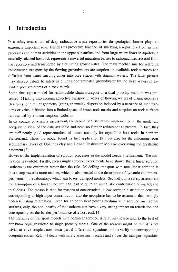
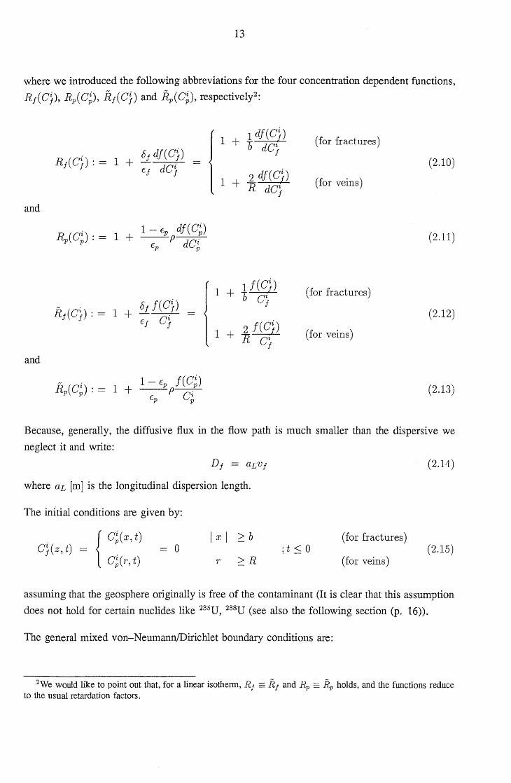
In the first representation (see also Figure la) we assume that the advective/dispersive flux takes

place in z-direction within a fissure with constant aperture 2b.

x

z

z = 0 (Inlet)

maximal

~llllllllllillllt.b.Penetration depth D

i fracture half-width b

z=L (Outlet)

Figure la: The (x, z)-geometry for transport in a fracture zone.

The inlet is at z = 0 and we assume that the contaminant is uniformly distributed over the whole

width of the fracture. Within the fracture ground water moves with a constant velocity Vj.

8

In reality fractures are neither planar nor do they extend as single fractures over the distances to

be considered. The effect of a system of interconnected fractures is simulated by a dispersion

which is taken into account by a longitudinal dispersion length aL' Sorption of the radionuclides

onto fissure surfaces is governed by a non-linear isothenn.

Matrix diffusion removes the contaminant from the water conducting zone in the x--direction,

perpendicular to the direction of the advective/dispersive flux, into connected porosity. The

transport in the x--direction is assumed to be purely diffusive and with no advective component

because of the very low hydraulic conductivity. The rock matrix accessible to diffusion is limited,

be it by symmetry considerations (half the distance to the next fracture) or by a limited extent

of interconnected pore spaces (limited matrix diffusion). Within the pores the nuclides sorb

and the sorption isothenn may be again a non-linear one. Additionally, we assume radioactive

decay and, in the case of a nuclide chain, decay of the precursor. This simple scenario for our

model represents, for example, contaminant flow in fractured dykes of aplite and pegmatite in

the crystalline [2] but also flow in other geological features such as "crushed zones" or larger

conductive layers [3].

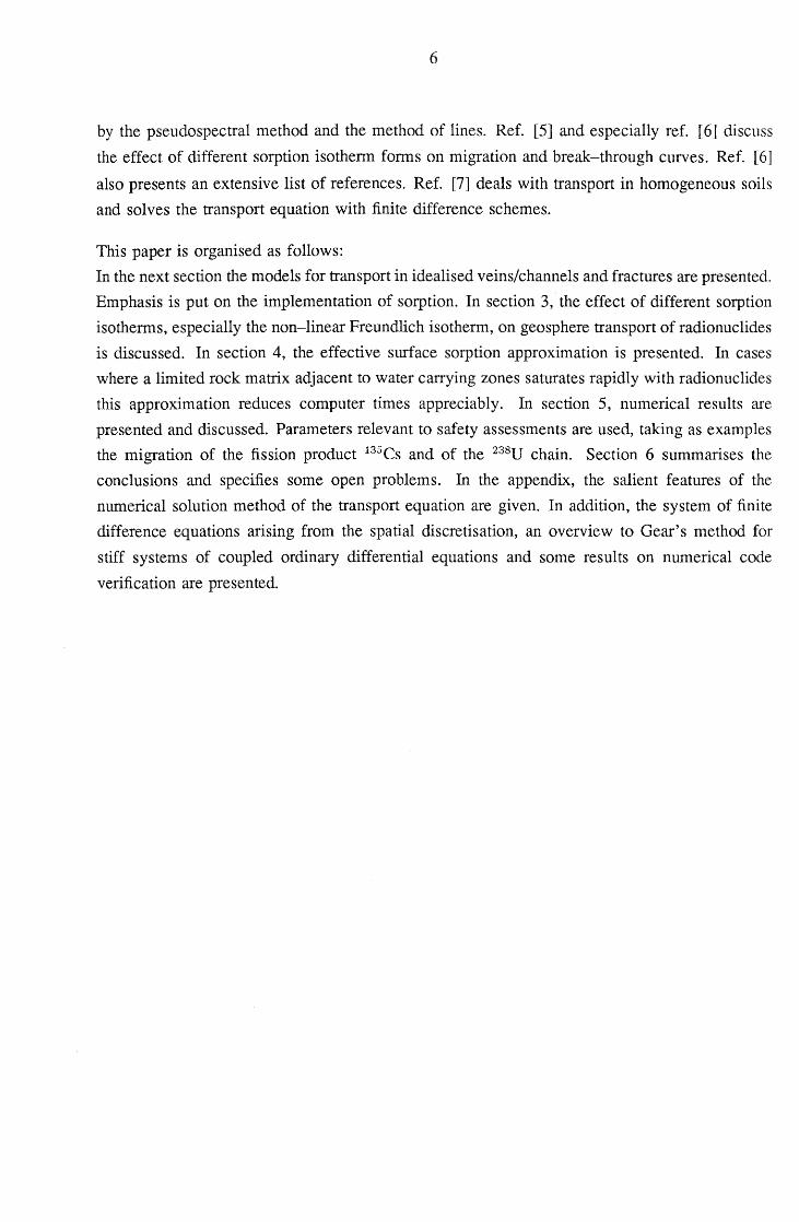
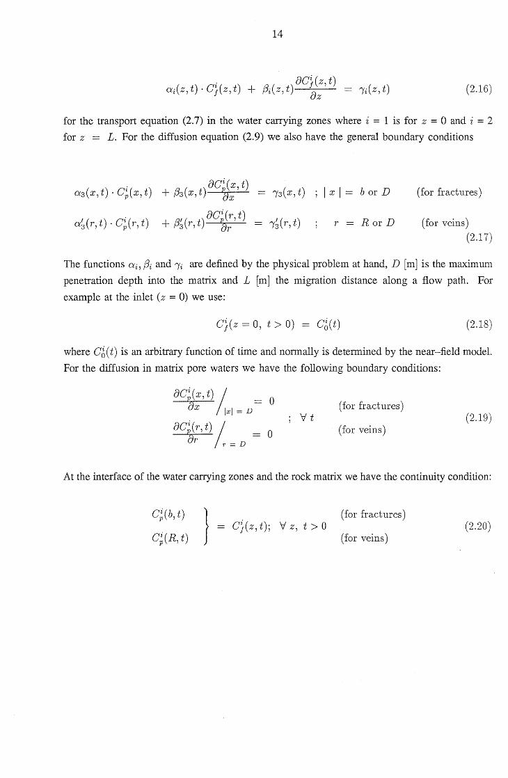
The alternative geometry is sketched in Figure Ib, where flowpaths are veins or channels and

are modelled by tubes of a constant radius R. The relevant physical mechanisms are the same

as specified in the previous case.

z=O (Inlet)

z=L (Outlet)

Figure Ib: Model of the (r, z)-geometry in the case of transport in veins.

9

Some remarks to the concept of the REV

A microscopic description of the radionuclide transport is not feasible due to the lack of know­

ledge on the geometrical structures. It is also not possible to describe in an exact mathematical

manner all the relevant physical/chemical processes between the host rock and the moving ra­

dionuclides.

But, fortunately, we are not interested in the microscopic distribution of the contaminant and,

following Bear [8], [9], the concept of the Representative Elementary Volume REV is intro­

duced. The actual (microsopic) quantities are replaced by (macroscopic) continuum quantities

by averaging over the REV. The size of such a REV strongly depends on geometry of the solid

phase and represents the smallest possible volume which contains the full geometrical complex­

ity of the system. Or in other words: The REV is this minimum volume of material over which

a physical quantity can be averaged such that its value is not sensitive to small variations of

the size of the REV. Practically it is not easy to determine the size of a REV and it is very

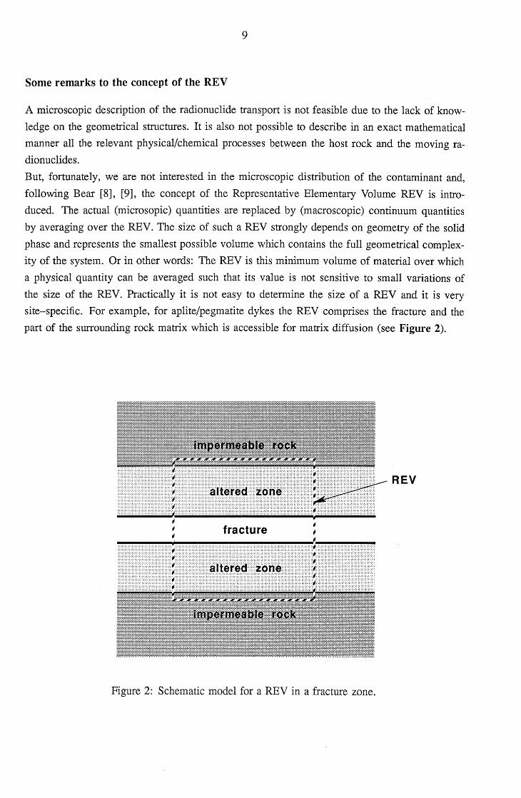
site-specific. For example, for aplite/pegmatite dykes the REV comprises the fracture and the

part of the surrounding rock matrix which is accessible for matrix diffusion (see Figure 2).

REV

fracture

Figure 2: Schematic model for a REV in a fracture zone.

10

The transport equations

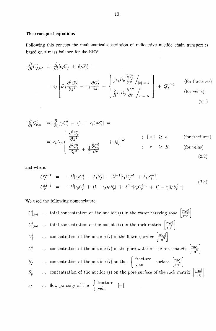
Following this concept the mathematical description of radioactive nuclide chain transport is

based on a mass balance for the REV:

a . mCj,tot

a . OiC;,tot

and where:

8 . Oi[EpC; + (1 Ep)pS;]

1 a2

ci

W I x I ED + Q~,i-l

p p 82C~ 1~ r

8r2 + r r

_,,\i [EfC} + bfS}] + ,,\i-l [Ef C;-1 + b fS;-I]

> b

> R

_,,\i[EpC; + (1 - Ep)pS;] + ,,\i-l[EpC;-1 + (1 - Ep)pS;-I]

We used the following nomenclature:

(for fra.ctures)

(for veins)

(2.1)

(for fra.ctures)

(for veins)

(2.2)

(2.3)

C}.tot total concentration of the nuclide (i) in the water carrying zone [:~ll

C;.tot total concentration of the nuclide (i) in the rock matrix [:~ll

C} concentration of the nuclide (i) in the flowing water [:~ll

C; concentration of the nuclide (i) in the pore water of the rock matrix [:~ll

concentration of the nuclide (i) on the {fr~cture surface [m~ll veIn In

S; concentration of the nuclide (i) on the pore surface of the rock matrix [k~ll

flow porosIty of the . . { fracture veIn

[-]

11

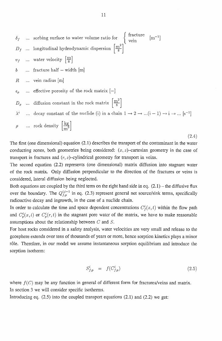
sorbing surface to water volume ratio for {fr~cture [m- 1 ] veIn

longitudinal hydrodynamic dispersion [ms2]

Vj water velocity [~]

b fracture half - width [m]

R vein radius [m]

tp effective porosity of the rock matrix [-]

Dp diffusion constant in the rock matrix [~2]

Ai decay constant of the nuclide (i) in a chain 1 -+ 2 -+ ... (i - 1) -+ i -+ ... [S-I]

P rock density [~] (2.4)

The first (one dimensional) equation (2.1) describes the transport of the contaminant in the water

conducting zones, both geometries being considered: (x, z)-cartesian geometry in the case of

transport in fractures and (r, z)-cylindrical geometry for transport in veins.

The second equation (2.2) represents (one dimensional) matrix diffusion into stagnant water

of the rock matrix. Only diffusion perpendicular to the direction of the fractures or veins is

considered, lateral diffusion being neglected.

Both equations are coupled by the third term on the right hand side in eq. (2.1) - the diffusive flux

over the boundary. The QY:p-l in eq. (2.3) represent general net source/sink terms, specifically

radioactive decay and·ingrowth, in the case of a nuclide chain.

In order to calculate the time and space dependent concentrations C} ( z, t) within the flow path

and C;(x, t) or C;(r, t) in the stagnant pore water of the matrix, we have to make reasonable

assumptions about the relationship between C and S.

For host rocks considered in a safety analysis, water velocities are very small and release to the

geosphere extends over tens of thousands of years or more, hence sorption kinetics plays a minor

role. Therefore, in our model we assume instantaneous sorption equilibrium and introduce the

sorption isotherm:

S~,p (2.5)

where f (C) may be any function in general of different form for fractures/veins and matrix.

In section 3 we will consider specific isotherms.

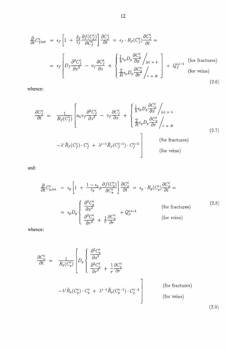
Introducing eq. (2.5) into the coupled transport equations (2.1) and (2.2) we get:

{) . mCj,tot

whence:

and:

whence:

12

[1 §.L a f( Cj)] Dff} . DC;

Ej + Ej aCj t = Ej' Rj(Cj)Tt =

1

aci

1 [ 1 ~ Tt Rp(C;) Dp a2ei 1 aei W +-;T

_).i~(C;). C; + ).i-1~(C;-1). C;-l 1

(for fractures) + Qji-l

(for veins)

(for fractures)

(for veins)

(for fractures)

(for veins)

(for fractures)

(for veins)

(2.6)

(2.7)

(2.8)

(2.9)

13

where we introduced the following abbreviations for the four concentration dependent functions,

R,(C}), Rp(C;), R,(C}) and Rp(C;), respectively2:

1 + 1 df(C~) (for fractures) b dCz 8, df(C}) ,

R,(C}) : = 1 + (2.10) dCi c, ,

.:£ df( C~) 1 + R dC2 (for veins) ,

and

Rp(C;) : = 1 + 1 - Cp df(C;) (2.11) --p .

cp dC;

1 + 1 f(CD (for fractures) b C2

8, f(C}) , R,(C}) : = 1 + (2.12) Ci c, ,

:£f(CD 1 + R C2 (for veins) ,

and

Rp(C;) : = 1 + 1 - cp f(C;) (2.13) --p-.-

cp C;

Because, generally, the diffusive flux in the flow path is much smaller than the dispersive we

neglect it and write:

(2.14)

where aL [m] is the longitudinal dispersion length.

The inItial conditions are given by:

I x I ? b (for fractures) o ·t < 0 , - (2.15)

r ?R (for veins)

assuming that the geosphere originally is free of the contaminant (It is clear that this assumption

does not hold for certain nuclides like 235U, 238U (see also the following section (p. 16)).

The general mixed von-NeumannlDirichlet boundary conditions are:

2We would like to point out that, for a linear isothenn, R j == Rj and Rp == Rp holds, and the functions reduce to the usual retardation factors.

14

8C}(z, t) ai(Z, t) . C}(Z, t) + (3i(Z, t) 8z = ri(Z, t) (2.16)

for the transport equation (2.7) in the water carrying zones where i = 1 is for Z = 0 and i = 2

for z = L. For the diffusion equation (2.9) we also have the general boundary conditions

a3 ( x, t) . C; ( x, t) + (33(X, t) ac~~, t) = r3(X,t) I x 1= b or D (for fractures)

a~ ( r, t) . C; ( r, t) (3' ( ) aC~r, t) r~(r, t) r R or D (for veins) + 3 r, t r (2.17)

The functions ai, (3i and ri are defined by the physical problem at hand, D [m] is the maximum

penetration depth into the matrix and L [m] the migration distance along a flow path. For

example at the inlet (z = 0) we use:

C}(z = 0, t > 0) = C~(t) (2.18)

where C~(t) is an arbitrary function of time and normally is determined by the near-field model.

For the diffusion in matrix pore waters we have the following boundary conditions:

(for fractures) Vt (2.19)

(for veins)

At the interface of the water carrying zones and the rock matrix we have the continuity condition:

C;(b, t)

C;(R, t) } = Cj ( z, t); V z, t > 0

(for fractures) (2.20)

(for veins)

15

3 The Effect of Sorption on Mass Transport - Retardation

In many cases [2],[12] an important mechanism retarding nuclide migration from a repository

is the diffusion of radionuc1ides from a water-conducting zone into pores of the rock matrix

(matrix-diffusion), see also ref. [10], [11] and therein. There, they may be sorbed onto the

surfaces of the pores and microfissures and may undergo radioactive decay. Matrix diffusion

is intrinsically included in our model and we restrict the discussion in this section to sorption

processes.

Sorption onto the solid phases (fracture/vein surfaces, inner matrix surfaces) constitutes the main

retardation mechanism for migrating radionuc1ides. In general the sorption and the desorption

behaviour is dependent on the element, its speciation in liquid phase, its concentration and also

on the characterisation of the solid phase. Well known phenomenological relationships between

concentration in the liquid phase and on the solid phase have been given (among others) by

Henry, Freundlich and Langmuir (see also refs. [13], [14], [15]). For practical purposes, the

underlying thermodynamical concepts are rarely helpful.

We will only present results for a Freundlich isotherm in the following sections. However, for

completeness and better understanding, we shall also make some remarks about the linear and

the Langmuir isotherm.

For sorption equilibrium the three different isotherms have the following form:

a) linear isotherm : Sl =](·e (3.1)

b) Freundlich isotherm : SF =](. eN N > 0 (3.2)

c) Langmuir isotherm : Smax' e (3.3)

where ](, N, Smax are empirical constants.

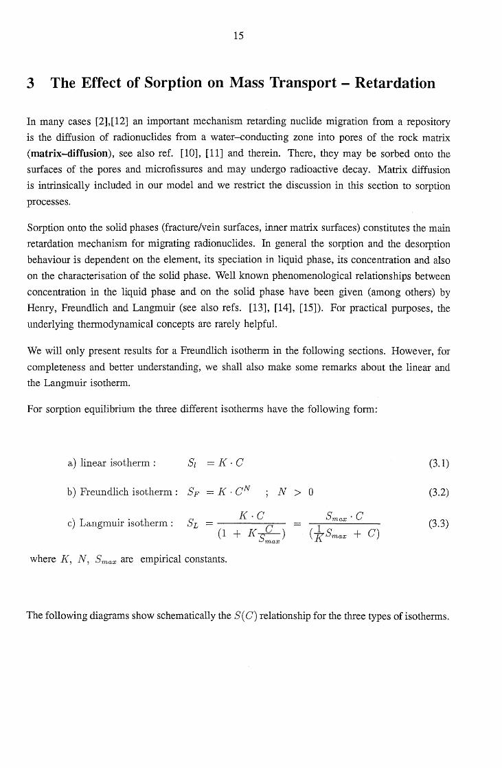
The following diagrams show schematically the S( C) relationship for the three types of isotherms.

16

5 (C) F

C C C

linear isotherm Freundlich isotherm Langmuir isotherm

Figure 3: Schematic diagrams for the three types of isotherms

For low concentration C <t: Smax the Langmuir isotherm has a linear behaviour and for high

concentration, S (C) becomes a constant = Smax, the saturation concentration.

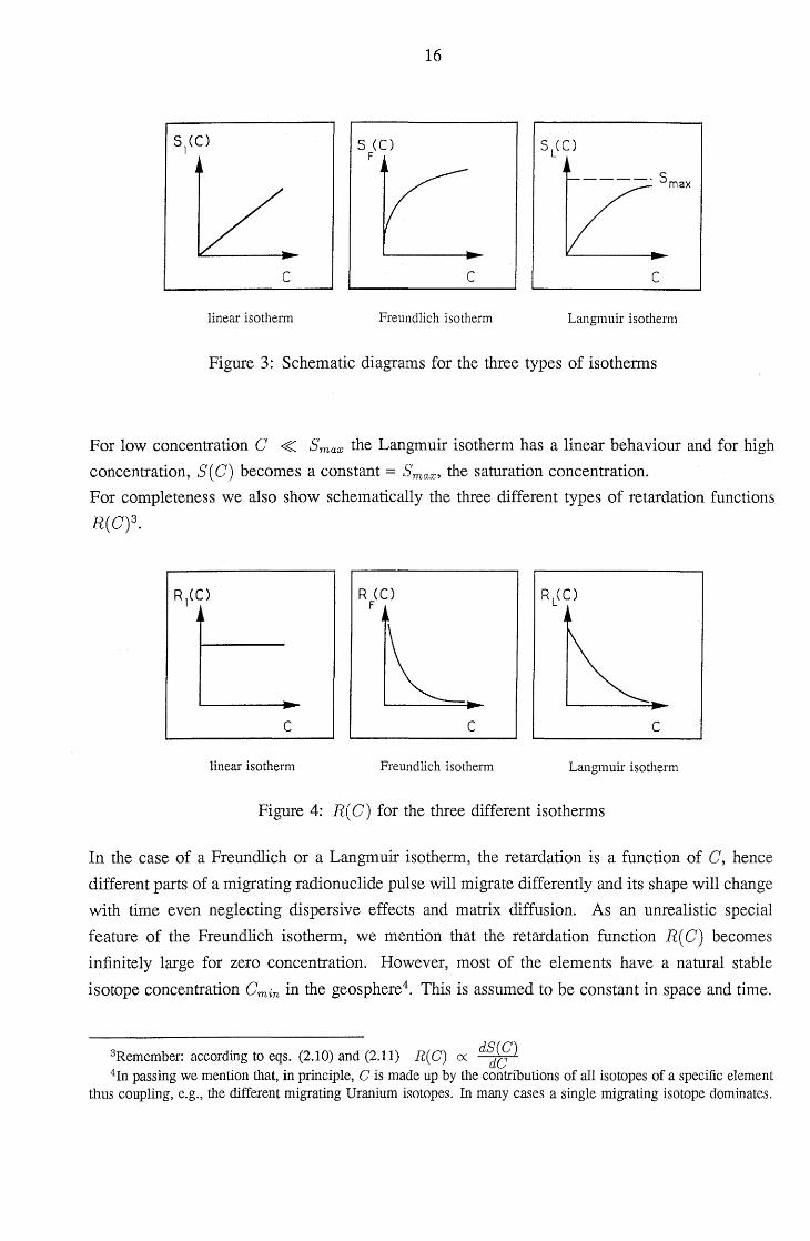
For completeness we also show schematically the three different types of retardation functions

R(C)3.

.. C

linear isotherm

R (C) F

C

Freundlich isotherm

C

Langmuir isotherm

Figure 4: R( C) for the three different isotherms

In the case of a Freundlich or a Langmuir isotherm, the retardation is a function of C, hence

different parts of a migrating radio nuclide pulse will migrate differently and its shape will change

with tirne even neglecting dispersive effects and matrix diffusion. As an unrealistic special

feature of the Freundlich isotherm, we mention that the retardation function R( C) becomes

infinitely large for zero concentration. However, most of the elements have a natural stable

isotope concentration Cmin in the geosphere4• This is assumed to be constant in space and time.

3Remember: according to eqs. (2.10) and (2.11) R(C) ex d~cg) 4In passing we mention that, in principle, C is made up by the contributions of all isotopes of a specific element

thus coupling, e.g., the different migrating Uranium isotopes. In many cases a single migrating isotope dominates.

17

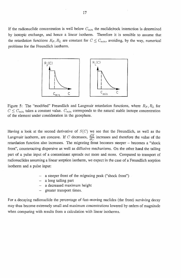
If the radionuclide concentration is well below Cmin the nuclide/rock interaction is determined

by isotopic exchange, and hence a linear isotherm. Therefore it is sensible to assume that

the retardation functions RF , RL are constant for C S Cmin , avoiding, by the way, numerical

problems for the Freundlich isotherm.

R (C) F

C

Figure 5: The "modified" Freundlich and Langmuir retardation functions, where RF, RL for C S Cmin takes a constant value. Cmin corresponds to the natural stable isotope concentration of the element under consideration in the geosphere.

Having a look at the second derivative of S( C) we see that the Freundlich, as well as the

Langmuir isotherm, are concave. If C decreases, ~ increases and therefore the value of the

retardation function also increases. The migrating front becomes steeper - becomes a "shock

front", counteracting dispersive as well as diffusive mechanisms. On the other hand the tailing

part of a pulse input of a contaminant spreads out more and more. Compared to transport of

radionuclides assuming a linear sorption isotherm, we expect in the case of a Freundlich sorption

isotherm and a pulse input:

a steeper front of the migrating peak ("shock front") a long tailing part a decreased maximum height greater transport times.

For a decaying radionuclide the percentage of fast-moving nuclides (the front) surviving decay

may thus become extremely small and maximum concentrations lowered by orders of magnitude

when comparing with results from a calculation with linear isotherms.

18

4 Effective Surface Sorption Approximation

When the diffusion into the rock matrix is sufficiently fast such that the concentration in the

connected pore spaces in the matrix adjusts "instantaneously" to the concentration in the water

carrying zones, diffusion into the matrix and sorption on matrix surfaces can be represented by

an effective surface sorption on fracture or on vein surfaces. In ref. [1] it has been shown for

transport in fractures what "instantaneously" means in quantitative terms. Therefore we assume,

for the following, a priori that5

\fz, xVr, t > O.

For the sorption isotherms in the fractures/veins and matrix respectively we define again:

fj( C})

fp( C})

(4.1 )

(4.2)

(4.3)

For cylindrical geometry we can write down the transport equation, without loss of generality,

for a nuclide which is not produced from a decaying parent:

a. (R) 2 { a2 C} ac} } .. at C;ot = D Dj az2 - Vj az - )..~C;ot ( 4.4)

Again, D is the maximal penetration depth for matrix diffusion, R the vein radius and (R/ D)2

is the ratio of volume of water carrying zone to total volume.

In eq. (4.5) the first term relates to the concentration in the veins, the second to the concentration

on vein surfaces; the third term is proportional to the nuclide concentration in the stagnant pore

water of the matrix whereas the last term is the contribution of the concentration on the matrix

pore surfaces.

Inserting eq. (4.5) into (4.4) and rearranging terms yields

5Intuitively it seems evident that eq (4.1) holds if Rp(C}). D2jDp is a sufficiently small time, where Cj is an

average concentration in the water carrying zones.

19

Comparing eqs. (4.6) and (2.6) shows that sorption on matrix surfaces can be treated as an

effective surface sorption if

(4.7)

where c is an arbitrary constant. For a Freundlich isotherm, e.g., this requires N j = Np' In the

expressions for Rj(C}) and Rj(Cj), eq. (2.10) and (2.12) the following replacements have to

be made on the right hand side

1---+1 + ( 4.8)

and

( 4.9)

As a side remark we note the well known fact6 that also non-sorbing tracers are retarded by

matrix diffusion and the retardation factor Rm .d. is given by

(4.10)

So, for example, with values of Cp = 0.033, D = 0.5 m and R = 5 . 10-3 m from ref. [1] a

retardation factor of Rm .d. = 331 is calculated.

For planar geometry of the water carrying zones the transport equation is

(4.11)

Again, eq. (4.7) is a necessary condition for an effective surface sorption approximation. In

the expressions for Rj(Cj ) and Rj(C}), eqs. (2.10) and (2.12) the following replacements now

have to be made

(4.12)

6This effect is also important for dating groundwaters with "ideal" tracers ([16], [17], [18]) and has especially large consequences for radioactive tracers when half-lives are smaller than tracer transport times.

20

and

( 4.13)

Inspecting eqs. (4.8), (4.9), (4.12) and (4.13) one will recognize that, besides the magnitude of

sorption given by the isotherm Jp ( C}), it is the ratio of matrix pore volume to water carrying

zone's volume which determines retardation by matrix diffusion. Without knowing the maximal

penetration depth D little can be said whether vein or fracture flow systems are more conservative

in a repository safety analysis.

We have shown under which conditions, assuming equilibrium (eq. (4.1)), matrix diffusion

can be approximated by an effective surface sorption. The advantage is a massive reduction

in computer time and space, especially for a large number of scoping calculations. To what

extent assumption (4.1) is fulfilled remains a question difficult to answer. However, it is always

possible to make a conservative estimate of a maximal penetration depth D.

21

5 Results and Discussion

In this section we present numerical results for the solution of the equations presented in the

previous sections.

For the choice of the input parameters we take into account two considerations:

1. the parameters should clearly show the impact of the non-linear sorption isotherm on break-through curves and

2. the results should be relevant to a safety assessment of deep geological disposal.

For high-level radioactive waste one option is disposal into the crystalline basement of northern

Switzerland. (The investigations have recently been extended to . overlaying sedimentary rocks.)

A comprehensive safety analysis has been performed some years ago [2]. Therefore, our cal­

culations will refer to this analysis. The selection of radionuclides was influenced by recently

documented sorption data from uranium and cesium [19], [20] from batch sorption and, in the

case of uranium, also from a dynamic experiment [21]. Both, U and Cs, exhibit a non-linear

sorption behaviour. The most important reason for choosing 135CS is the fact, that this nuclide

made up 95 % of the total dose to man [2], assuming a conservatively chosen linear sorption

isotherm. Considering the more realistic (non-linear) sorption behaviour of 135CS, a considerably

lower dose to man is expected.

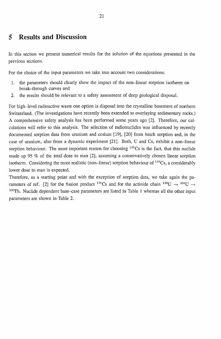
Therefore, as a starting point and with the exception of sorption data, we take again the pa­

rameters of ref. [2] for the fission product 135CS and for the actinide chain 238U -+ 234U -+

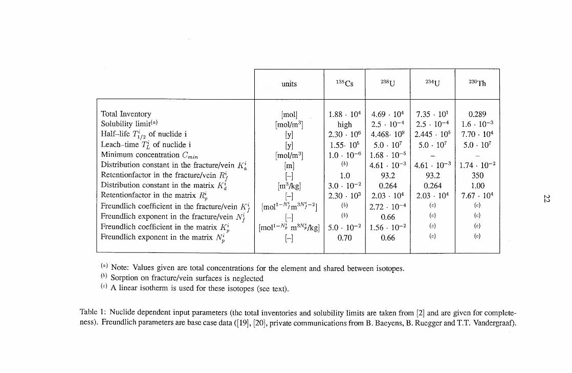
230Th. Nuclide dependent base-case parameters are listed in Table 1 whereas all the other input

parameters are shown in Table 2.

units 135CS 238U

Total Inventory [mol] 1.88 . 104 4.69 . 104

Solubility limit{a) [mol/m3] high 2.5 . 10-4

Half-life T{/2 of nuclide i [y] 2.30 . 106 4.468. 109

Leach-time TI of nuclide i [y] 1.55· 105 5.0 . 107

Minimum concentration Cmin [mol/m3] 1.0 . 10-6 1.68 . 10-5

Distribution constant in the fracture/vein I{i [m] (b) 4.61 . 10-3 a

Retentionfactor in the fracture/vein R} [-] 1.0 93.2 Distribution constant in the matrix I{~ [m3/kg] 3.0 . 10-2 0.264 Retentionfactor in the matrix R~ [-] 2.30 . 103 2.03 . 104

Freundlich coefficient in the fracture/vein I{} [mol1- N}m3N}-2] (b) 2.72 . 10-4

Freundlich exponent in the fracture/vein N} [-] (b) 0.66 Freundlich coefficient in the matrix I{i [mol1-N~ m3N;/kg] 5.0 . 10-2 1.56 . 10-2

p

Freundlich exponent in the matrix N i p [-] 0.70 0.66

(a) Note: Values given are total concentrations for the element and shared between isotopes. (b) Sorption on fracture/vein surfaces is neglected (c) A linear isotherm is used for these isotopes (see text).

234U 230Th

7.35 . 101 0.289 2.5 . 10-4 1.6 . 10-3

2.445 . 105 7.70 . 104

5.0 . 107 5.0 . 107

- -

4.61 . 10-3 1.74 . 10-2

93.2 350 0.264 1.00

2.03 . 104 7.67 . 104

(c) (c)

(c) (c)

(c) (c)

(c) (c)

Table 1: Nuclide dependent input parameters (the total inventories and solubility limits are taken from [2] and are given for complete­ness). Freundlich parameters are base case data ([19], [20], private communications from B. Baeyens, B. Ruegger and T.T. Vandergraat).

N N

Site characterisation and nuclide independent parameters: Migration distance L Water velocity v j Dispersion length a L

Diffusion constant of altered zone Dp Porosity of altered zone cp Density of altered zone p = p(1 - cp) Water flow through the repository Q L

Hydraulic conductivity J{

Hydraulic gradient \71> Fracture frequency n j; vein frequency nv Fracture half-width b; vein radius R Maximal penetration depth D

Boundary conditions: Up-stream (i = 1) Down-stream(i = 2)(a)

Release scenario:

Integration data: Order of the interpolation polynomial in flow direction Number of discretisation points in flow direction Order of the interpolation polynomial in matrix-diffusion direction Number of discretisation points in matrix-diffusion direction

units

[m] [m/y] [m]

[m2/s] [-]

[kg/m3] [m3/y] [m/s] [-]

[m-l]; [m-2]

[m] [m]

for fractures for veins

500 0.473 I 6.03

50 1.515 . 10-11

3.3 . 10-2

2530 4.2

1.25 .10- 9

0.012 10 1

5 . 10-5 5 .10-3

10-3 0.5

ai f3i Ii 1 0 1 1 0 0

Reference [22]

3 3 26 (equidistant)

3 31 (equidistant)

3 15 (equidistant) 58 (not equidistant)

(a) This down-stream boundary condition represents a strong dilution of the contaminant by an overlaying aquifer.

Table 2: Base case input parameters for both alternative geometries (Parameters are from [2]).

tv w

24

At the inlet, the input (boundary) concentration is given by the following expression:

C}(z = 0, t) .- C~(t) (5.1)

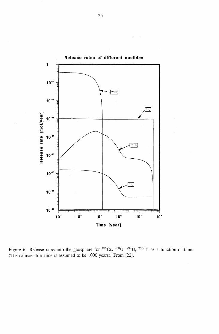
where Ri(t) is the (normally) time-dependent release rate of nuclide i into the geosphere. It is

taken from [22] and shown for completeness in Figure 6.

QL is the total water flow through the repository, assumed to be 4.2 m3/y:

(5.2)

where t [-] is the average porosity of the repository region, F [m2] is the repository cross­

section and v f is the water velocity [m/y].

At the down-stream boundary, the results of the calculations are presented as normalised nuclide

flows, defined by:

Jtot (z = L, t) . - J. (- L t) QL .- norm Z - ,

8Ci j -t . Vf . F . aL __ f

8z z-Tt

(5.3)

25

Release rates of different nuclides

1

10.01

1135Csl

10.02

...... ... ca

10.03 CD >-........ 0 E ...... CD 10.04 .... ca ... CD f/)

ca 10.05 CD

CD a:

10.08

10.07

1 0.08 ~---P~"""'~---P-I-"""'~~~"""'I"'I'I'I--""I'~"""'~---P"""""'''''''

1 03

Time [year]

Figure 6: Release rates into the geosphere for 135CS, 238U, 234U, 230Th as a function of time. (The canister life-time is assumed to be 1000 years). From [22].

26

Effects of the spatial discretisation

To test the convergence behaviour of the spatial discretisation in the flow and matrix diffusion

directions we have done serveral calculations for fracture flow and vein flow systems. The

starting point for these investigations are the base case integration data given in Table 2.

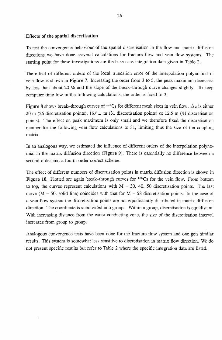
The effect of different orders of the local truncation error of the interpolation polynomial in

vein flow is shown in Figure 7. Increasing the order from 3 to 5, the peak maximum decreases

by less than about 20 % and the slope of the break-through curve changes slightly. To keep

computer time low in the following calculations, the order is fixed to 3.

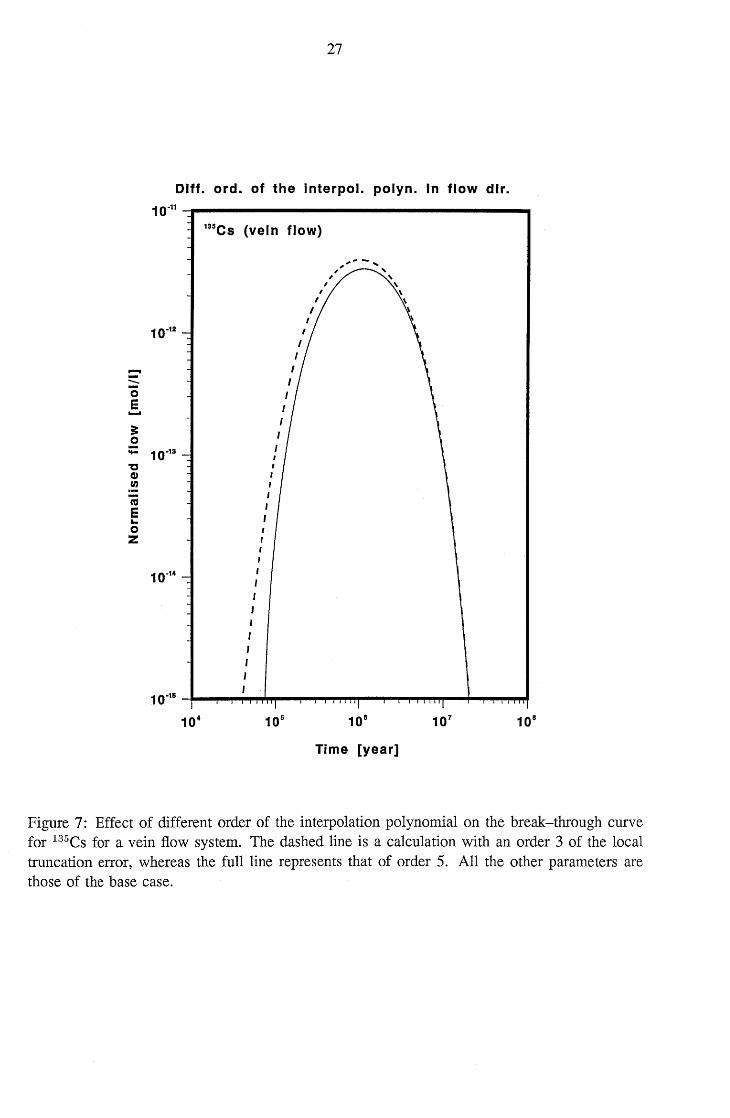
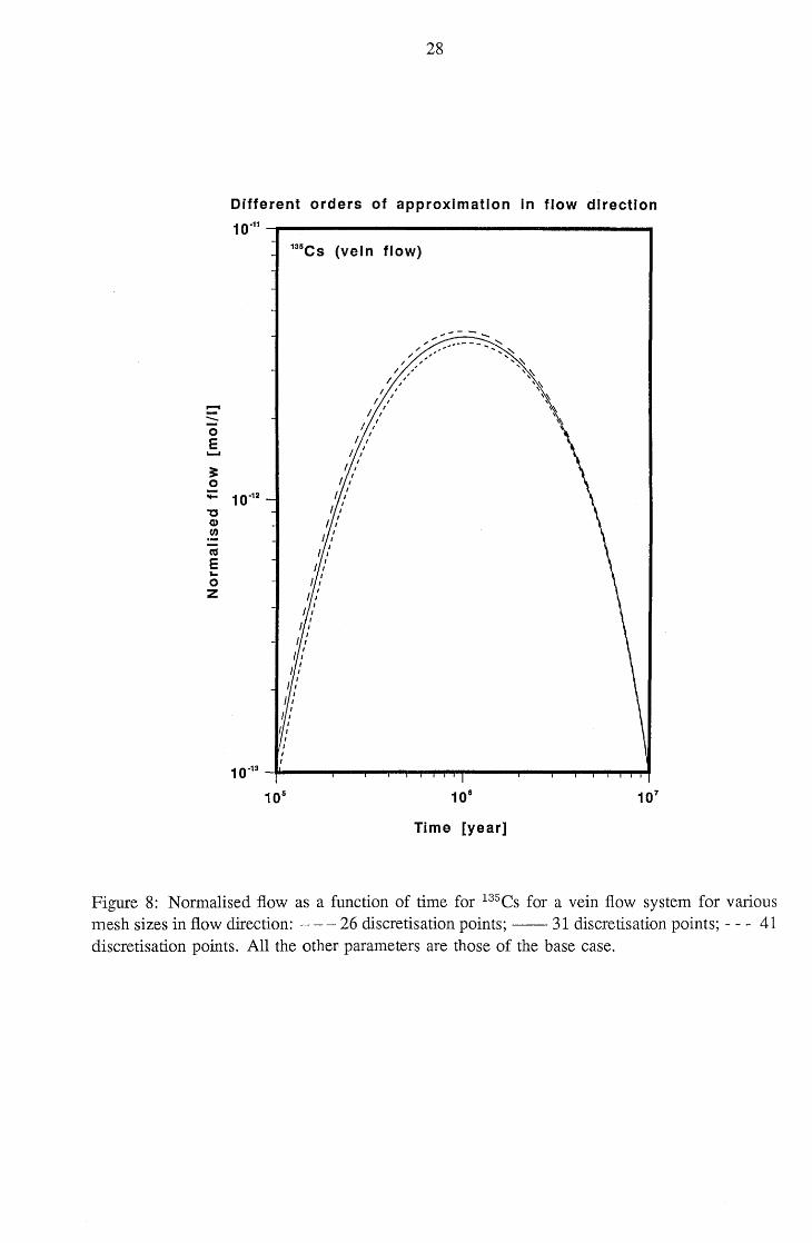
Figure 8 shows break-through curves of 135CS for different mesh sizes in vein flow. 6.z is either

20 m (26 discretisation points), 16.6 ... m (31 discretisation points) or 12.5 m (41 discretisation

points). The effect on peak maximum is only small and we therefore fixed the discretisation

number for the following vein flow calculations to 31, limiting thus the size of the coupling

matrix.

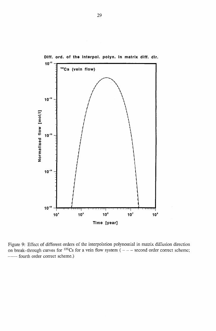
In an analogous way, we estimated the influence of different orders of the interpolation polyno­

mial in the matrix diffusion direction (Figure 9). There is essentially no difference between a

second order and a fourth order correct scheme.

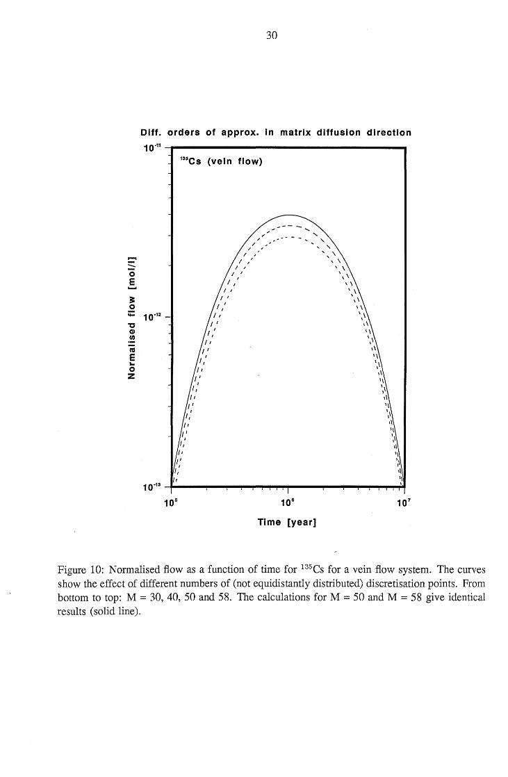
The effect of different numbers of discretisation points in matrix diffusion direction is shown in

Figure 10. Plotted are again break-through curves for 135CS for the vein flow. From bottom

to top, the curves represent calculations with M = 30, 40, 50 discretisation points. The last

curve (M = 50, solid line) coincides with that for M = 58 discretisation points. In the case of

a vein flow system the discretisation points are not equidistantly distributed in matrix diffusion

direction. The coordinate is subdivided into groups. Within a group, discretisation is equidistant.

With increasing distance from the water conducting zone, the size of the discretisation interval

increases from group to group.

Analogous convergence tests have been done for the fracture flow system and one gets similar

results. This system is somewhat less sensitive to discretisation in matrix flow direction. We do

not present specific results but refer to Table 2 where the specific integration data are listed.

27

Diff. ord. of the Interpol. polyn. in flow dlr.

10.11 -r--------------------. 135CS (vein flow)

10.12

..... -0 E ..... ;:: 0 ;: 10.13

'C G) tn

as I E .... I 0 I

Z , , , 10.14 I

I I I

I I

Time [year]

Figure 7: Effect of different order of the interpolation polynomial on the break-through curve for 135CS for a vein flow system. The dashed line is a calculation with an order 3 of the local truncation error, whereas the full line represents that of order 5. All the other parameters are those of the base case.

28

Different orders of approximation In flow direction

10.11 -p----------------------. 135CS (vein flow)

...... -0 E ..... == 0 :;: 10.12

"0 CI.)

tJJ

C'CI

E ... 0 z

Time [year]

Figure 8: Normalised flow as a function of time for 135CS for a vein flow system for various mesh sizes in flow direction: - - - 26 discretisation points; -- 31 discretisation points; - - - 41 discretisation points. All the other parameters are those of the base case.

29

Dlff. ord. of the Interpol. polyn. In matrix diff. dir.

10.11 --p--------------------. 13SCS (vein flow)

10.12

...... -0 E ...... :: 0 - 10.13

"C CD t/)

ca E .. 0 Z

10.14

Time [year]

Figure 9: Effect of different orders of the interpolation polynomial in matrix diffusion direction on break-through curves for 135CS for a vein flow system ( - - - second order correct scheme; -- fourth order correct scheme.)

-..... 0 E ......

== 0 ;:

'0 CI) fI)

ca E .. 0 z

30

Dlff. orders of approx. in matrix diffusion direction

10.11 -p-------------------...... 135CS (vein flow)

.;

/;' ~~.--

/ " / '

I "

I " I ,

I ' / I

I

10.12

.. , .... \

, \ \ \

\\ \ \

\ \ \

\\

/1 '\ 1 0.13 -f----P'--!"'" ............ ..,..,..., ...... ---P"-' ...... -,........., ...... ~I

Time [year]

Figure 10: Normalised flow as a function of time for 135CS for a vein flow system. The curves show the effect of different numbers of (not equidistantly distributed) discretisation points. From bottom to top: M = 30, 40, 50 and 58. The calculations for M = 50 and M = 58 give identical results (solid line).

31

5.1 Fracture flow system

In this subsection we present results for 135CS transport in a fracture flow system. The base case

parameters are specified in Tables 1 and 2.

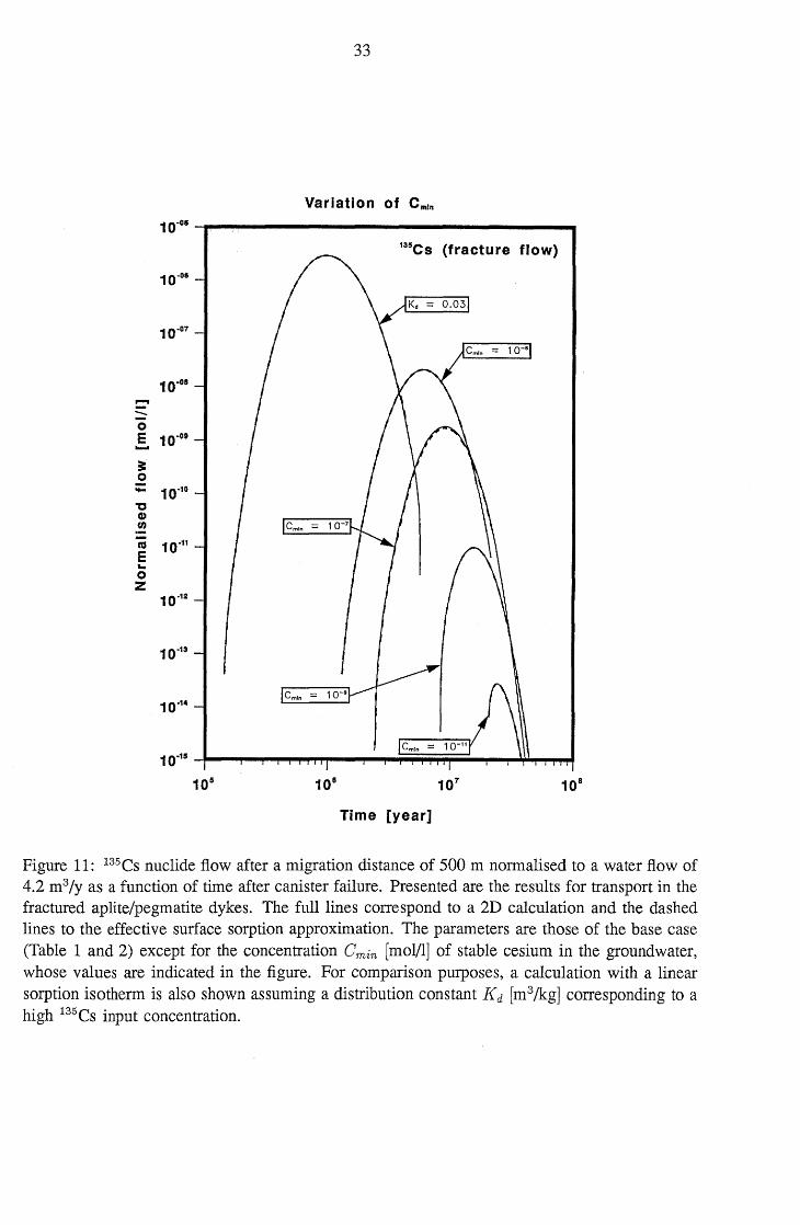
Consideration of the non-linear sorption behaviour of cesium has a strong impact on nuclide

outflow from the host rock. However, the magnitude is largely dependent on the background

concentration of natural cesium in the groundwaters. For crystalline waters natural cesium

concentrations from detection limit up to around 10-5 mol/l have been given [23], [24]. The

upper values are measured in higher mineralised waters. In order to see the full impact of a

non-linear isotherm we have chosen a base case value at the lower end, Cmin = 10-9 mol/l,

and varied the parameter in a broad range. This is illustrated in Figure 11. The lower this

natural concentration, the larger the concentration range with non-linear sorption, the steeper the

front of migrating 135CS and the less survival of fast moving nuclides: Hence, the variation of

nuclide flow over about six orders of magnitude. Even for a high natural cesium concentration,

consideration of the non-linearity of sorption reduces outflow when compared with the result

with a linear isotherm sorption coefficient chosen according to the maximum input concentration

of 8.6 . 10-5 mol/l. In that case, most of the 135CS nuclei survive transport. Also shown in

Figure 11 is the excellent agreement of the effective surface sorption approximation with the

full two-dimensional calculation. This is a consequence of the very limited volume of available

rock matrix for diffusion and the rapid equilibration between matrix pore and fracture waters.

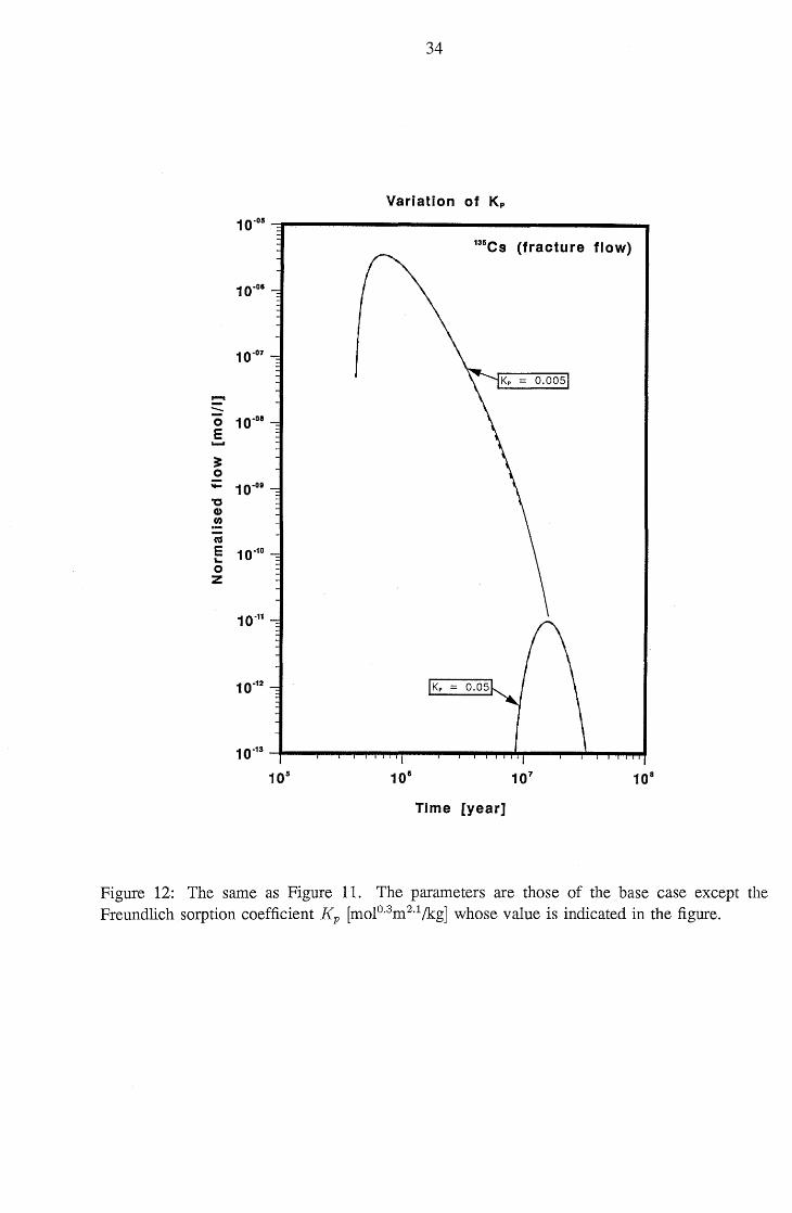
Figure 12 shows the dependence on the Freundlich coefficient for sorption in the matrix. For

the lower value of I{p, retardation is small and most nuclides survive transport. For the higher

value of I{p, retardation is roughly an order of magnitude larger and transport times are large

compared to half-life. Again, the effective surface sorption approach constitutes an excellent

approximation.

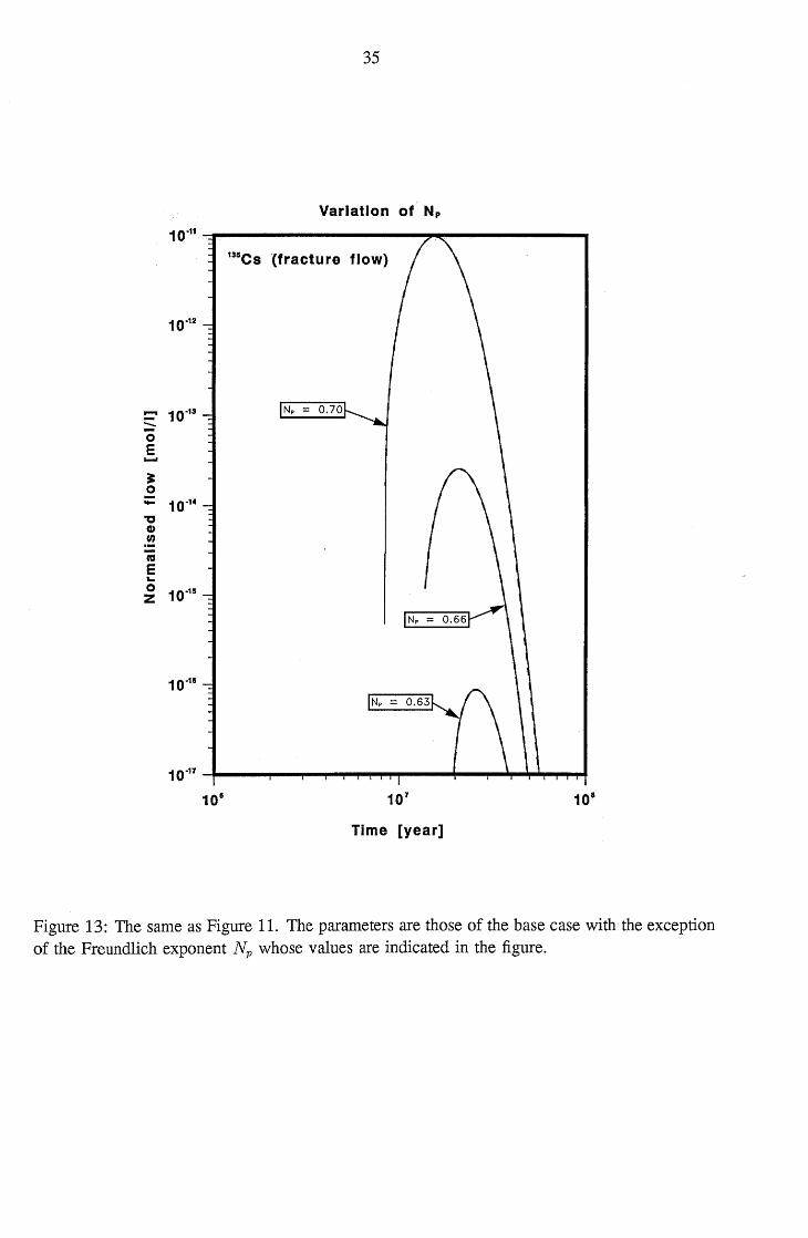
When transport times are large compared to half-life, the magnitude of the Freundlich exponent

Np becomes extremely important (Figure 13). For lower Np, with a marked non-linearity, the

migration fronts are steeper and the percentage of fast moving nuclides much lower. Hence, with

a decrease of the Freundlich exponent by 10% one gets a reduction of outflow by five orders of

magnitude. Again, the effective surface sorption approximation is an excellent approximation

for the reasons mentioned above.

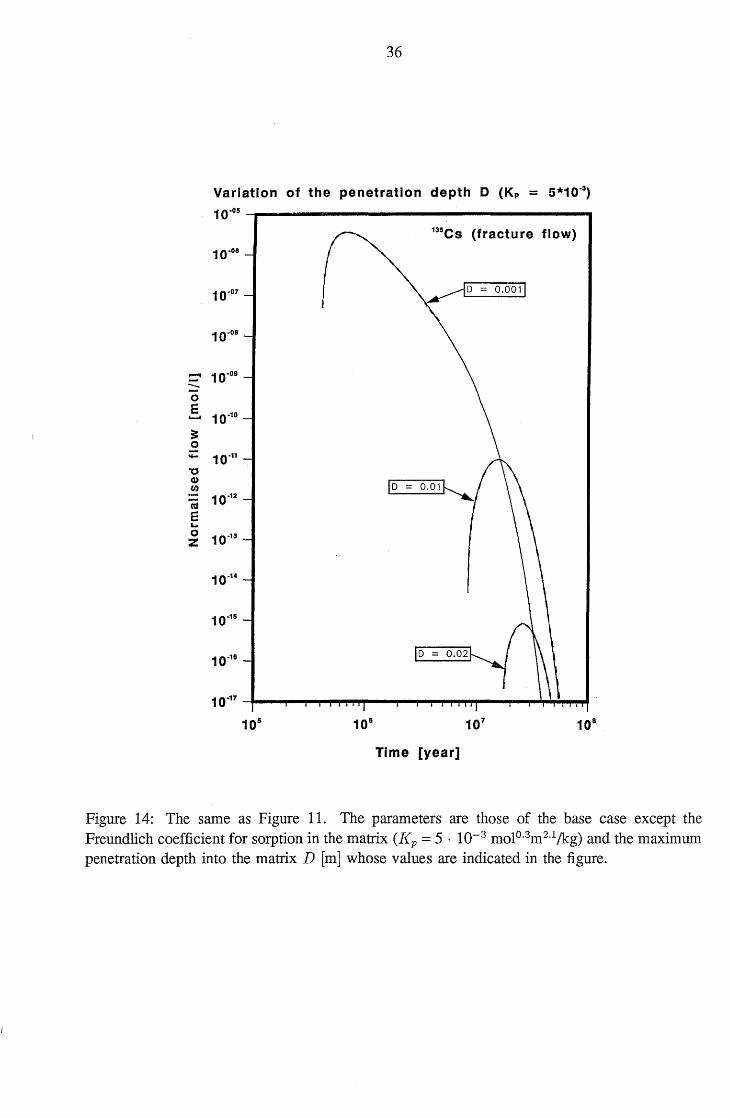
The retardation for transport in the fracture flow system is strongly dependent on the matrix

volume available for diffusion and sorption. This is shown in Figure 14. Here, the calculations

were performed with a low Freundlich parameter I{p since no outflow results for the base case I{p

and maximum penetration depths D 2:: 0.01 m. For the values leading to the results of Figure 14,

32

the matrix is rapidly saturated with 135CS and, hence, the effective surface approximation is

an excellent approach. Clearly then, the retardation is directly proportional to the maximum

penetration depth D and, for residence times larger than half-live, a strong dependency of

maximal outflow on D results.

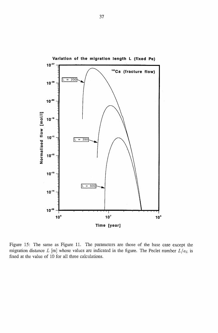
Keeping all other parameters fixed the residence time is directly proportional to the migration

distance L if the rock matrix is saturated. This is the case for the results presented in Figure 15.

In these calculations the Peclet number L / aL was held constant. Smaller dispersivities and

longer transport paths, both, lead to a strong decrease of nuclide outflow if residence times are

large compared to half-life, as is here the case.

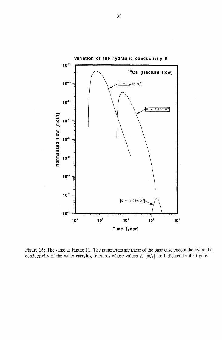
A similar influence on nuclide outflow results from a variation of water velocity v J (Figure 16).

The hydraulic conductivity ]( has been increased up to two orders of magnitude from the base

case keeping hydraulic gradient and flow porosity constant. For the highest water velocity, all of

the 135CS nuclei survive transport and peak outflow almost corresponds to peak inflow. The peak

reduction for the intermediate water velocity results to a larger extent from increased dispersion

when residence time increases and to a lesser extent from radioactive decay. For the base case

water velocity, radioactive decay becomes extremely important.

33

Variation of Cmln

10.05

135CS (fracture flow)

10.05

10.07

10.08

.... ::::-0 E 10.011 ...... ~ 0 :;: 10.10

"C CD In

ca 10.11

E .. 0 Z

10.12

10.13

10.14

10.15

105

Time [year]

Figure 11: 135CS nuclide flow after a migration distance of 500 m normalised to a water flow of 4.2 m3/y as a function of time after canister failure. Presented are the results for transport in the fractured aplite/pegmatite dykes. The full lines correspond to a 2D calculation and the dashed lines to the effective surface sorption approximation. The parameters are those of the base case (Table 1 and 2) except for the concentration Cmin [moW] of stable cesium in the groundwater, whose values are indicated in the figure. For comparison purposes, a calculation with a linear sorption isotherm is also shown assuming a distribution constant I{d [m3/kg] corresponding to a high 135CS input concentration.

34

Variation of Kp

10.05 -=r-------------------...

1315CS (fracture flow)

10.07

-::::-0 10.08

E .-

~ 0 :;: 10.011

"C CI) U)

C\'S

E 10.10 ... 0 Z

10.11

1 0.13 -i--...,..-.,....,..~'"'""'"'I""P_-...,.."""'""...,..~~,....-.....................

Time [year]

Figure 12: The same as Figure 11. The parameters are those of the base case except the Freundlich sorption coefficient I{p [molO.3m2

.1/kg] whose value is indicated in the figure.

35

Variation ot' Np

10.11 -:r-----------~!'-------....

135CS ,(fracture flow)

10.12

.... 10.13 -0 E -== 0 :;: 10.14

'C CD CI)

ca E .. 0 10.15 Z

1011

Time [year]

Figure 13: The same as Figure 11. The parameters are those of the base case with the exception of the Freundlich exponent Np whose values are indicated in the figure.

36

Variation of the penetration depth 0 (Kp = 5*10.3)

10.05

135CS (fracture flow) 10.08

10.07

10.08

..... 10.09 -0 E 10.10 .......

:= 0 = 10.11

"0 <I> th

CIS 10.12

E 1..0

0 10.13 Z

10.14

10'15

10.18

10.17

105 106 107 108

Time [year]

Figure 14: The same as Figure 11. The parameters are those of the base case except the Freundlich coefficient for sorption in the matrix (I{p = 5 . 10-3 molO.3m2.1/kg) and the maximum penetration depth into the matrix D [m] whose values are indicated in the figure.

37

Variation of the migration length L (fixed Pel

10.07 -::P---------------------.....

135CS (fracture flow)

10.011

-::::-0 10.10

E ..... ;: 0 ;: 10.11

"0 G> U)

ca E 10·1~ .. 0 Z

10.13

10.14

10.15 -t---.... - ......... ..,...,....,. ......... --..... ~~ ..................

108

Time [year]

Figure 15: The same as Figure 11. The parameters are those of the base case except the migration distance L [m] whose values are indicated in the figure. The Pee let number L/aL is fixed at the value of 10 for all three calculations.

38

Variation of the hydraulic conductivity K

10.04 -::r--------------------. 135CS (fracture flow)

1.25*10-7

10.06

1.25*10-8

-0 E

10.07

..... == 0 ;: 10.08

" (J) U)

C'CS

E 10.09 ... 0 Z

10.10

10.11

K 1.25*10-9

Time [year]

Figure 16: The same as Figure 11. The parameters are those of the base case except the hydraulic conductivity of the water carrying fractures whose values I{ [m/s] are indicated in the figure.

39

5.2 V~in flow system

The results presented in this subsection (figures 17 to 22) illustrate the main features of geosphere

transport in a (r, z )~geometry. Again transport of 135 CS is taken as an example and the impact

of some parameter variations is investigated.

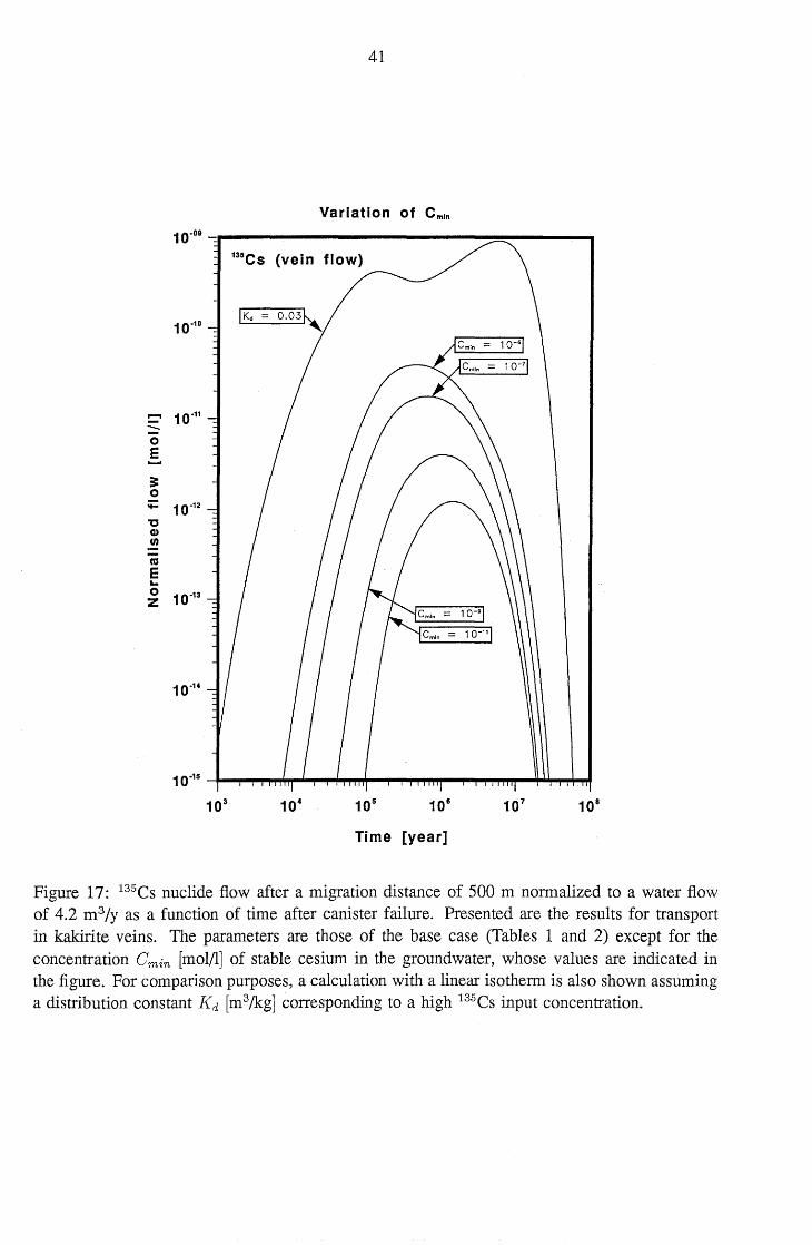
Figure 17 shows the effect of varying the natural cesium concentration on the break-through.

On a lower outflow level- because available rock mass for matrix diffusion is much larger - the

effect is less pronounced than for fracture flow (see figure 11). Loosely speaking, the nuclide

outflow is determined by nuclides transported mainly in the veins and not the bulk of nuclides,

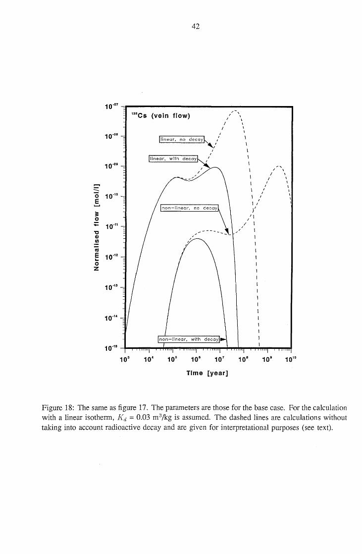
which diffuse into and sorb in the rock matrix decaying there to insignificance. This can be

seen in Figure 18 where, for interpretation purposes, the radioactive decay has been switched

off (dashed line) and the strong retardation potential of matrix diffusion as well as the effect of

decay (full lines) is clearly seen. In Figure 17, again, the results taking into account non-linear

sorption are compared to the corresponding results for a linear isotherm. This curve led to the

base case dose calculation in "Project Gewtihr 1985" [2, fig. 14-1]. It should be noted that

consideration of a non-linear isotherm for 135 Cs reduces total doses in that safety assessment by

a factor of 25 even for the large natural cesium background of 10-6 mol/l, and the contribution

of cesium to almost negligible amounts.

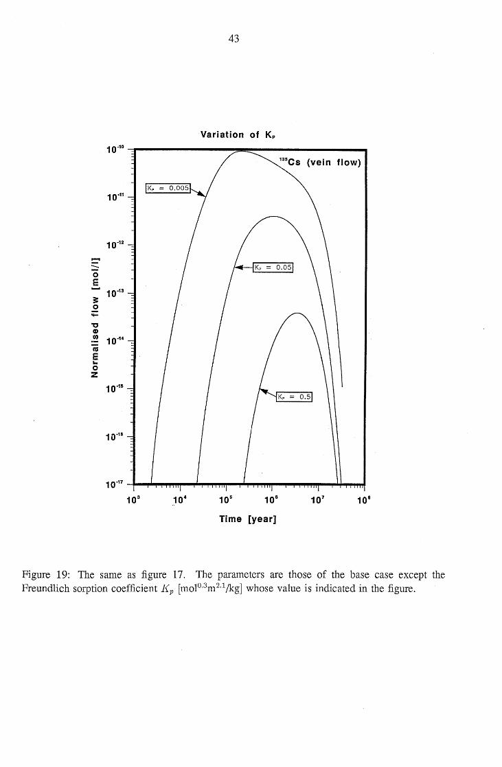
In Figure 19 the effect of varying the Freundlich coefficient on nuclide flow is presented. Again,

for vein flow the impact is less pronounced on a lower outflow level compared to fracture flow

(Figure 12). The reasons are the same as discussed above: The main portion of nuclides diffus­

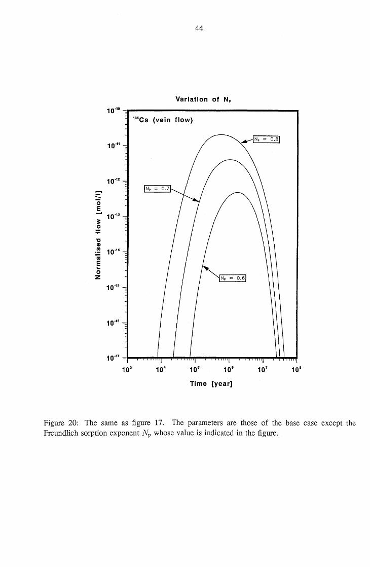
ing into and out of the matrix decay to insignificance. The same situation is seen when varying

the Freundlich exponent (Figure 20) and comparing to Figure 13.

For practical applications in safety assessments, it is pleasing to see that the parameter dependen­

cies are much less for vein flow than for fracture flow. However, this is mainly a consequence

of the much larger matrix pore volume available for diffusion in the first flow system: The

overwhelming majority of cesium nuclides diffuse into the rock matrix and decay there. The

kind of sorption mechanism in the matrix plays little role and is felt in the geosphere outflow

indirectly, only, through the coupling of the two transport equations.

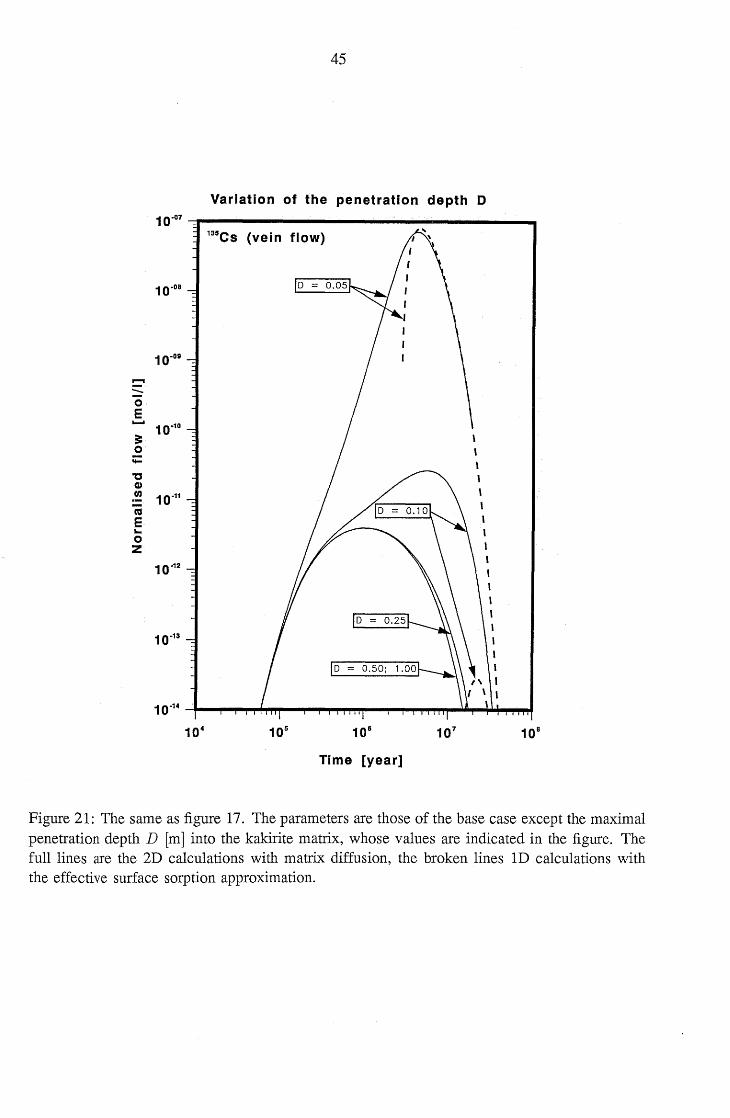
Figure 21 presents the influence of maximal penetration depth for diffusion into the rock matrix.

For the two smallest values of D, the peak value is determined by nuclides moving into and out of

the matrix whereas for larger penetration depths the breakthrough is dominated by fast moving

nuclides in the water carrying zones (see discussion above). When comparing to Figure 14,

the main difference to the fracture flow system can bee seen: For vein flow the effect of

matrix diffusion on nuclide outflow is limited and reaches an asymptotic value. The reason

40

is the totally different geometry. So, for fracture flow, the volume available for diffusion is

directly proportional to the maximal penetration depth; for vein flow this volume increases with

the square of the maximal penetration depth and the diffusion equation has a totally different

structure. For the smallest value of D, the effective surface sorption approach constitutes a good

approximation but for larger values of D the matrix is not sufficiently rapidly saturated with

135CS and, consequently the effective surface sorption approximation fails.

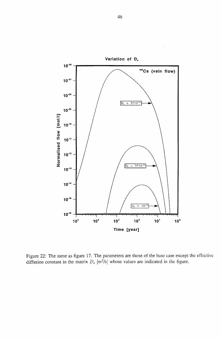
In Figure 22, the dependence on effective diffusion constant De is depicted. A lower value

of De than the base case value strongly restricts the effect of matrix diffusion, whereas for a

higher value more of the rock matrix is saturated more rapidly and the outflow values decrease

to insignificance.

41

Variation of Cmln

10.09 -:r-------------~~---......

135CS

- 10.11 -0 E ..... == 0 ;: 10.12

'tJ (I)

tn

C'CS

E .. 0 10.13 Z

Time [year]

Figure 17: 135CS nuclide flow after a migration distance of 500 m normalized to a water flow of 4.2 m 3Jy as a function of time after canister failure. Presented are the results for transport in kakirite veins. The parameters are those of the base case (Tables 1 and 2) except for the concentration Cmin [mol/l] of stable cesium in the groundwater, whose values are indicated in the figure. For comparison purposes, a calculation with a linear isotherm is also shown assuming a distribution constant ]{d [m3Jkg] corresponding to a high 135CS input concentration.

-0 E ........

== 0 :;:

"C CI) (J)

CO

E .. 0 z

42

10.07 -::p----------------------.

10.08

10.011

10.10

10.11

10.12

10.13

10.14

135CS (vein flow) ,-

/ ' \ I \

/ \

/ \

linear, with

Time [year]

/

,,/

\ \

\

\ 1

I 1 I

} I

,'1 / \

I I

I I

I

'" / \

/ \ \ ,

\ I , I I

Figure 18: The same as figure 17. The parameters are those for the base case. For the calculation with a linear isotherm, ]{d = 0.03 m3/kg is assumed. The dashed lines are calculations without taking into account radioactive decay and are given for interpretational purposes (see text).

43

Variation of Kp

10.10 -:r--------..,.~---------...

(vein flow)

10.12

--0 E ......

==

10.13

0 :;:

"0 CI) U) 10.14

Ct'I E .. 0 z

10.15

10.18

Time [year]

Figure 19: The same as figure 17. The parameters are those of the base case except the Freundlich sorption coefficient I{p [molO.3m2

.1/kg] whose value is indicated in the figure.

44

Variation of Np 10.

10 -.:p ________________ lllill-. __ -.

135CS (vein flow)

10.12

..... -0 E ......

10.13

;: 0 :;: -0 CD en 10.14

ctS E .. 0 Z

10.15

Time [year]

Figure 20: The same as figure 17. The parameters are those of the base case except the Freundlich sorption exponent Np whose value is indicated in the figure.

45

Variation of the penetration depth D

10.07 -=1"'----------------------....... 13Ses (vein flow)

10.011

.... -0 E ......

10.10

== 0 :;:

"C G) , rn 10.11

ca ,

E , ... , 0 , Z

10.12

Time [year]

Figure 21: The same as figure 17. The parameters are those of the base case except the maximal penetration depth D [m] into the kakirite matrix, whose values are indicated in the figure. The full lines are the 2D calculations with matrix diffusion, the broken lines 1Dcalculations with the effective surface sorption approximation.

46

Variation of D. 10.011

1315CS (vein flow)

10.07

10.011

10·01J

-0 E 10.10

-..

== 0 :;: 10.11

"C (I)

tn

ca 10.12

E .. 0 Z

10.13

10.14

10.15

10.111

103 104 105 106 10 7 10 6

Time [year]

Figure 22: The same as figure 17. The parameters are those of the base case except the effective diffusion constant in the matrix De [m2js] whose values are indicated in the figure.

47

5.3 Chain transport in the fracture flow system

In the present work, chain transport is investigated in much less detail than the transport of 135CS.

In fact, in the context of investigations of transport· of safety relevant nuclides with non-linear

sorption isotherms, the results presented are probably more of a mathematical exercise. The

reasons are manifold.

Let us first consider the choice of a relevant nuclide chain. The sorption behaviour of neptunium

is extremely complex [25], and we are not aware of an isotherm useful in the present context.

As an example we consider the 238U chain with the daughters 234U and 230Th. Very probably,

the deep groundwaters are already saturated with uranium, and there would be little uranium

release from the repository. Looking at the numbers, we have a natural concentration in granitic

groundwater [23] of 1.7 . 10-8 mol/l, a realistic uranium solubility limit [2] of 2.5 . 10-9 molll

and a conservative uranium solubility limit [2] of 2.5 . 10-7 mol/l. Calculations were done with

the value of 2.5 . 10-7 mol/l, leaving a little space for non-linear sorption behaviour. Reliable

uranium isotherms for reducing conditions and the solid phases of interest are not known to

the authors. For oxidising conditions, a measured isotherm for uranium(VI) sorption on Swiss

granite does exist [19]. For the sake of definiteness we have taken the measured Freundlich

exponent and reduced the Freundlich coefficient (Table 2) in order to take into account reducing

conditions. At this place we would like to point out a shortcoming of our transport code: It

is not possible to take into account the space and time dependent effect of concentration of a

migrating isotope on the sorption behaviour of all the other isotopes. For uranium, for example,

the natural element concentration Cmin is determined by 238U, whereas all the other isotopes can

be neglected. In the transport calculation for 238U, released from the repository, the effect of

Cmin on sorption is taken into account. But for sorption of 234U the time and space dependent

concentration of total 238U determines its sorption (both, natural and repository released contri­

butions).

As a conservative practical approximation we take for 234U a linear isotherm and fix the re­

tardation factor according to the maximum release rate of 238U (see Table 1). With all these

assumptions, chain calculations of Figure 23 cannot be much more than a mathematical exercise.

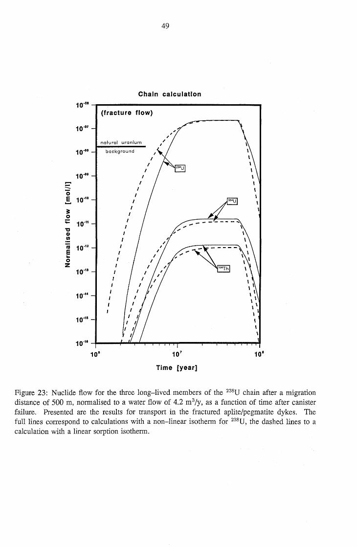
In Figure 23, a comparison between calculations with linear isotherms and with a non-linear

isotherm for 238U are made. Due to the long half-life and the extended repository release, 238U

outflow from the geosphere reaches its maximum corresponding to the solubility limit. Since the

I{ d for the linear sorption calculation was chosen according to this concentration, the outflow is

retarded somewhat more strongly in the non-linear sorption case. The effect however, is small

since the non-linearity of sorption is operative over a single decade of concentration values only.

The daughters 234U and 230Th have much shorter half-lives, they break-through in radioactive

48

equilibrium. Their maximum concentration is slightly enhanced in the non-linear sorption case,

since the ratio of retardation factors of 238U and 234U is slightly smaller than unity in the peak

flow region as a consequence from the approximation mentioned before. This difference also

shows the goodness of the approximation and its conservatism.

49

Chain calculation

10·oS

(fracture flow)

10.07

natural uranium

10.01 background

10.08 I - I

:::::- I 0 I E 10.10

I ...... it

I

0 I - 10.11 I

'C I

Q) I CI) I CO 10.12

E .. 0 Z I

10.13 I I I

10.14 I I I

10.15

10.11

10 1 107 101

Time [year]

Figure 23: Nuclide flow for the three long-lived members of the 238U chain after a migration distance of 500 m, normalised to a water flow of 4.2 m3/y, as a function of time after canister failure. Presented are the results for transport in the fractured aplite/pegmatite dykes. The full lines correspond to calculations with a non-linear isotherm for 238U, the dashed lines to a calculation with a linear sorption isotherm.

50

6 Conclusions

We have presented the governing equations for transport of radionuclides in inhomogeneous dual

porosity rocks taking into account non-linear sorption isotherms. The methods to solve these

equations and the approaches to verify the ensuing computer code RANCHMDNL have been

described.

For the case of a Freundlich isotherm, broad parameter variations based on values for a safety

assessment have been performed. Such an isotherm steepens the front of a migrating radionuclide

pulse. If transport times are around or larger than nuclide half-lives, only a small portion of the

radionuclides survive decay and nuclide outflow from the geosphere is strongly reduced when

compared to inflow. In these cases the results are heavily dependent on the parameter values

chosen. Especially noted is the change of cesium outflow by five orders of magnitude when

the Freundlich exponent is changed by 10 % in the fracture flow calculations. Also, apart from

this strong impact, it is evident from the results presented that considering the non-linearity of

isotherms reduces the nuclide outflow appreciably when comparing to the standard I{ d approach.

For the systems studied the main retardation is produced by matrix diffusion and sorption on

inner surfaces. If the available pore volume of rock matrix is sufficiently small and diffusion

sufficiently rapid, matrix diffusion can be described by an effective surface sorption.

The fracture flow system ((x,z)-geometry) is much more susceptible to parameter variations than

the vein flow system ((r,z)-geometry). This is a consequence of differing dependency of matrix

volume on the distance from water carrying zones and the different geometry of the interface

between these zones and the rock matrix.

After many years of investigations, the availability of useful and reliable sorption isotherms in

the context of safety assessments is still a problem. Cesium is, here, the notable exception.

Work is in progress along different lines. First, general isotherms will be included into the code.

This can be done relatively easily by full numerical calculation of the retardation functions based

on a tabulation of concentration in the solid versus concentration in the liquid phase. Second, the

model is currently being tested through application to results of laboratory experiments (dynamic

rock core infiltration and diffusion experiments). Foreseen is also its use in modelling the on­

going field migration experiments at N AGRA' s Grimsel Test Site. Third, an extension is planned

to deal with piecewise constant parameters along a migration path. This will allow modelling of

transport through layered systems, be it a series of sediments or a single host rock with spatially

varying properties.

51

7 Appendix:

Numerical Solution of the System of Non-linear Partial Differential Equations

Analytical solutions to the coupled system of eq. (2.7) and (2.9) are known only for very specific

retardation functions Rf(Cj), Rp(C;), Rf(Cj) and Rp(C;) (eq. (2.10) - (2.13)), linear sorption

isotherms, and simple boundary conditions. Therefore, it is necessary to solve the system of

equations numerically.

In principle, it is possible to get solutions by help of various numerical methods, such as finite

elements, finite differences or random walle Based on the experience [12] we use the method of

lines approximation. This method is a powerful tool to approximate the solution of initial value

problems for systems of linear and non-linear partial differential equations.

The method of lines is a semidiscretisation procedure where all independent variables but one

are discretisised. For every grid point (e.g. in the space domain) one gets one equation, which

means that every partial differential equation is converted into a system of ordinary differential

equations. This system of ordinary differential equations can then be solved by using standard

algorithms. Such standard algorithms are, for example, Bulers' s method or the method by Runge­

Kutta or various predictor-corrector methods (e.g. by Adams-Moulton, Adams-Bashforth).

There are algorithms with automatic control of the step size and for variable orders of the

expansion polynomial and procedures which keep truncation errors within a required accuracy.

A special method, used here, for solving ordinary differential equations has been developed

by Gear [26]. This algorithm is a multistep predictor/corrector method with all the advantages

mentioned above and is especially suitable in the treatment of stiff systems such as the coupled

transport equations.

Spatial discretisation and the system of finite difference equations

As mentioned before, in the method of lines approximation, the spatial variable is discretisised

whereas time is left continuous. First, we have to find a suitable approximation for spatial

derivatives. With the abbreviations 7

.-

.-C S

the system of transport equations can be written as

(A.1) (A.2)

7The quantity S, defined here, should not be confused with S, the concentration of sorbed nuclides as used in the previous sections.

52

(A.3)

(A.4)

Superscript (2) denotes the second derivative and superscript (1) the first derivative in z, x or

r depending on the specific equation at hand (see also eq. (2.7) and (2.9)). Lk abbreviate the

differential operators in space and Qk denote, again, sink/source terms. The coefficients aj and

(3j may be space and time dependent with:

aI, a3, /31, /32 > 0 a2 < 0

We look for a solution of eq (A.3) in the domain

OszSL ;Vt>O

and of eq. (AA) in the domain

(for fractures) (for veins)

(A.5) (A.6)

(A.7)

(A.8)

For the initial condition as well as for the (upstream-/downstream) boundary conditions we refer

the reader to section 2. Due to the continuity condition, eq. (2.20), both eq. (A.3) and (A.4)

are coupled.

In order to derive the piecewise polynomial approximation for the space dependency of the

functions C and S, we replace the two dimensional integration domain by a set of mesh points

in flow direction:

and in matrix-diffusion direction:

{ ; }:= {x} b (for fractures) R (for veins) , X2, """' Xj, Xj+l, """' XM = D }

(A.9)

(A. 10)

8We point out that in general the spacings .6.zi , .6.Xj i, j = 1,2, ... are not equidistant. The rectangular mesh is sketched below; the mesh points are labelled as indicated in the figure and for simplicity we assume (for the drawing) equidistant increments .6.zi and .6.Xj.

x,r=D

x=b r=R

'" x,r

M 2M

(M-I) (2M-I)

(M-2) (2M-2)

(M-3) (2M-3)

5 (M+5)

4 (M+4)

3 (M+3)

2 (M+2)

I (M+I)

z=o

3M

(3M-I)

(3M-2)

(3M-3)

(2M+5)

(2M+4)

(2M+3)

(2M+2)

(2M+ I)

53

= (Zi+l - Zi) = (Xj+l-Xj)

4M

(4M-I)

(3M+2)

(3M+I)

(N-2)xM (N-I )xM (NxM) -_e_---e---..

(NxM)-1 -_e_--_4_--..

- __ --~-__e (NxM)-2

(N-I )xM+3

(N-I )xM+2

(N-l )xM+ I . z=L z

Figure 24: Space mesh system and its numbering.

(A.II) (A.12)

The transformation of the two coupled partial differential equations into a set of coupled first

order ordinary differential equations can be done by Lagrange interpolation techniques.

For a set of given data points {Ui' Vi}, i = 1,2, ... , n and where (u, v) correspond either to (z, C)

or (x, S) and with Vi := V( Ui), we get for the (n-I)-th order interpolation polynomial Pn - 1:

n

v(u) ~ Pn-1(u) = I:Lk(U) . Vk (A.13) k=l

The Lagrange coefficients are given by:

(A.14)

with Lk(Uj) = Skj and Pn-1(Uk) = Vk.' Therefore the approximation polynomial Pn- 1 reproduces

exactly the functions C and S at the discretisation points.

For the first derivative we get:

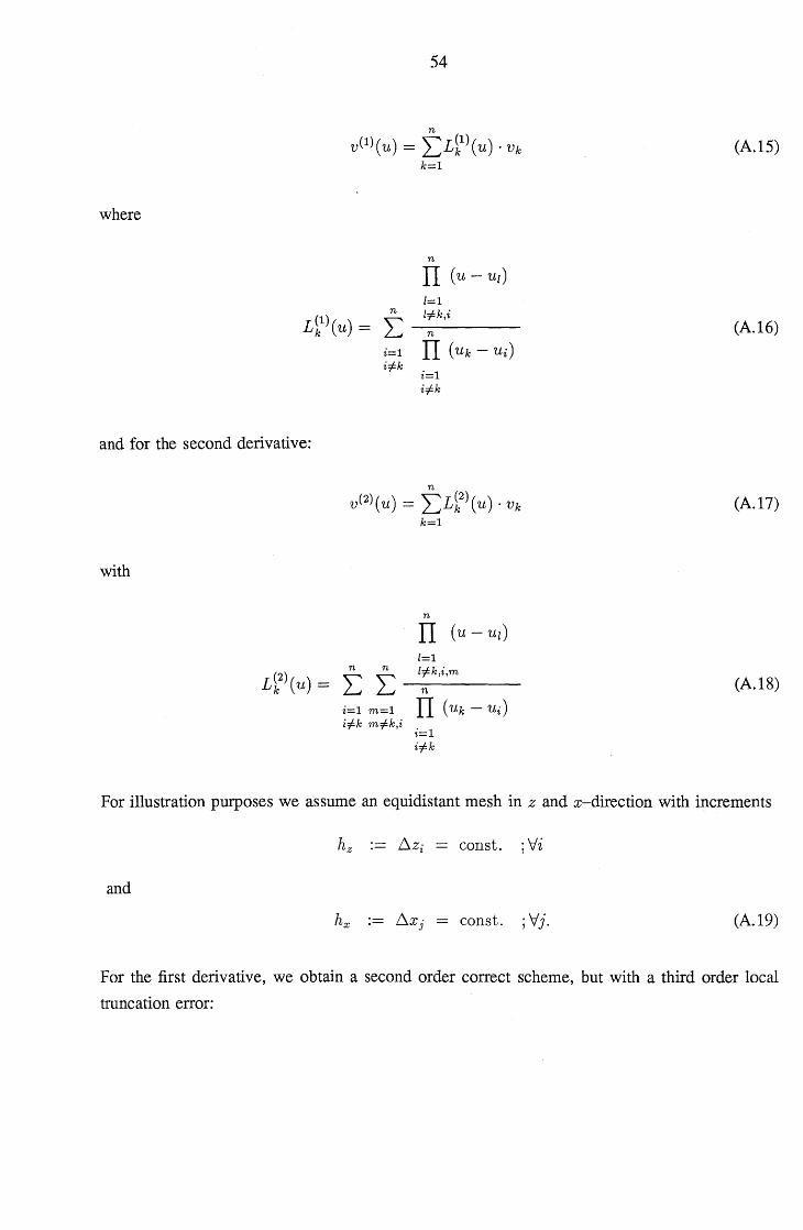
where

and for the second derivative:

with

54

n

V(l)(U) = I:L11)(U) . Vk

i=l i=lk

k=l

n

IT (u - UI) [=1

i=l i=lk

n

V (2) ( U) = I: L 12) ( u) . V k

k=l

n

IT (u - UI) [=1

n n l=lk,i,m L12)(u) = I: I: -n---

i=l m=l IT (Uk - Ui) i=lk m=lk,i

i=l i=lk

(A.15)

(A.I6)

(A.I?)

(A.I8)

For illustration purposes we assume an equidistant mesh in z and x-direction with increments

hz :== ~Zi == canst. ; Vi

and

canst. ; Vj. (A. 19)

For the first derivative, we obtain a second order correct scheme, but with a third order local

truncation error:

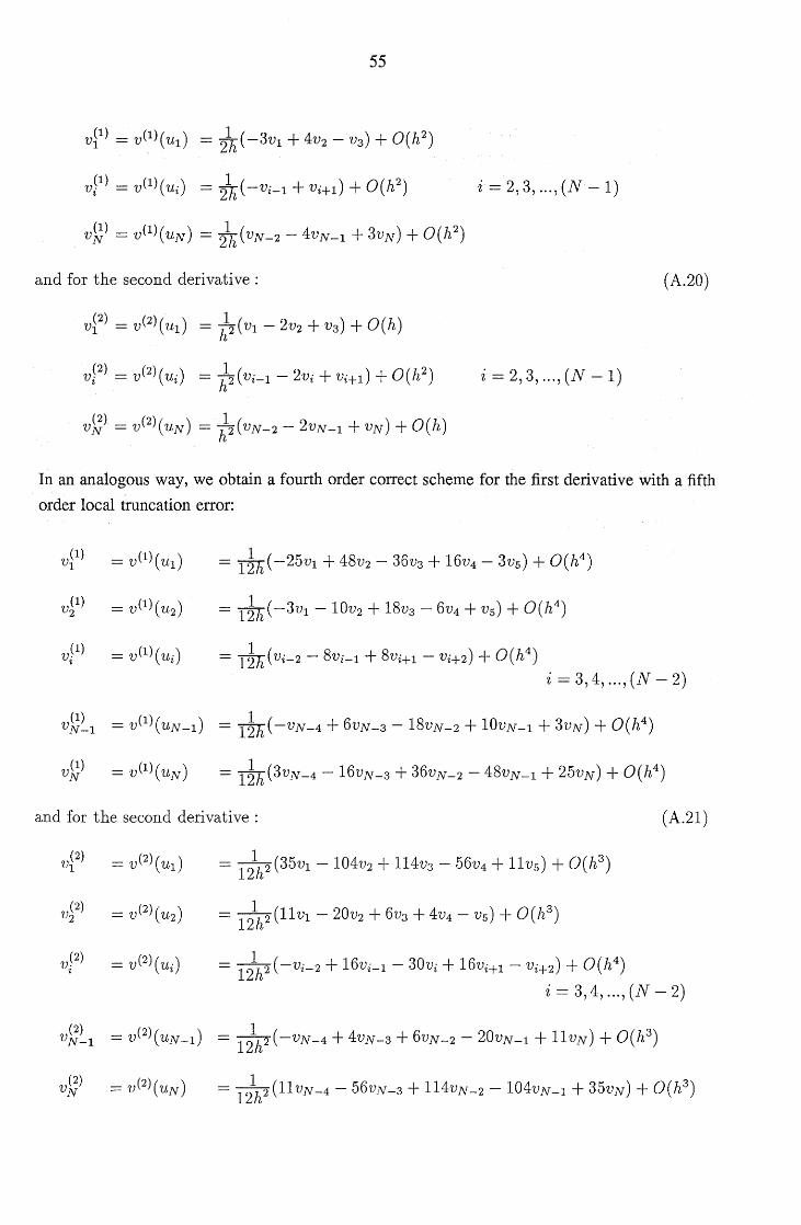
55

vP) = V(I)(UI) = lh (-3VI + 4V2 - V3) + O(h2)

VP) = V(I)(Ui) = -d7i( -Vi-I + Vi+l) + O(h2)

V~) = V(l)(UN) = 2\ (VN-2 - 4VN-l + 3VN) + O(h2)

and for the second derivative:

i=2,3, ... ,(N-1)

(A.20)

i=2,3, ... ,(N-l)

In an analogous way, we obtain a fourth order correct scheme for the first derivative with a fifth

order local truncation error:

= 1~h(-25vl + 48v2 - 36v3 + 16v4 - 3vs) + O(h4)

= l~h (-3VI - 10v2 + 18v3 - 6V4 + vs) + O(h4)

= l~h (Vi-2 - 8Vi-l + 8Vi+l - Vi+2) + 0 (h4) i=3,4, ... ,(N-2)

and for the second derivative:

= 121h2 (35vl - l04v2 + 114v3 - 56v4 + 11vs) + O(h3)

= 121h2 (llvl - 20V2 + 6V3 + 4V4 - vs) + O(h3)

= 12\2 (-Vi-2 + 16vi-l - 30Vi + 16vi+l - Vi+2) + O(h4)

(A.21)

i = 3,4, ... ,(N -2)

56

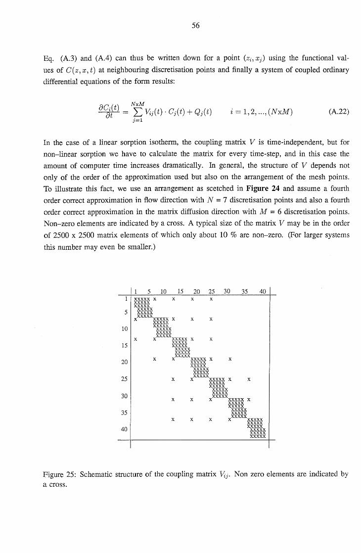
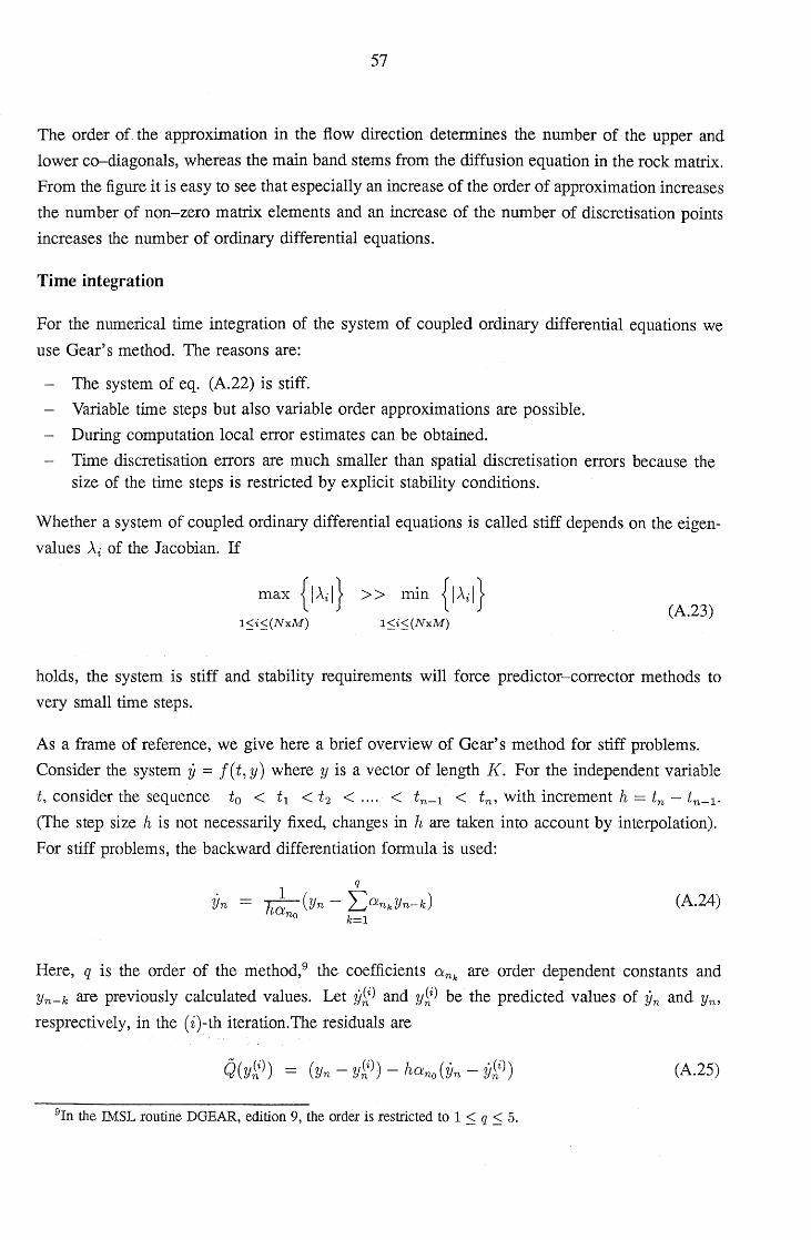
Eq. (A.3) and (A A) can thus be written down for a point (Zi, Xj) using the functional val­

ues of C (z, x, t) at neighbouring discretisation points and finally a system of coupled ordinary

differential equations of the form results:

i = 1,2, ... , (NxM) (A.22)

In the case of a linear sorption isotherm, the coupling matrix V is time-independent, but for

non-linear sorption we have to calculate the matrix for every time-step, and in this case the

amount of computer time increases dramatically. In general, the structure of V depends not

only of the order of the approximation used but also on the arrangement of the mesh points.

To illustrate this fact, we use an arrangement as scetched in Figure 24 and assume a fourth

order correct approximation in flow direction with N = 7 discretisation points and also a fourth

order correct approximation in the matrix diffusion direction with M = 6 discretisation points.

Non-zero elements are indicated by a cross. A typical size of the matrix V may be in the order

of 2500 x 2500 matrix elements of which only about 10 % are non-zero. (For larger systems

this number may even be smaller.)

5

10

15

20

25

30

35

40

1 5 10 15 20 25 30 35 40 xxxxx x x x x xxxxx xxxxx xxxxx xxxxx xxxxx x xxxxx x x x xxxxx xxxxx xxxxx xxxxx xxxxx x x xxxxx x x xxxxx xxxxx xxxxx xxxxx xxxxx x x xxxxx x x xxxxx xxxxx xxxxx xxxxx xxxxx x x xxxxx x x xxxxx xxxxx xxxxx xxxxx xxxxx x x x xxxxx x xxxxx xxxxx xxxxx xxxxx xxxxx x x x x xxxxx xxxxx xxxxx xxxxx xxxxx xxxxx

Figure 25: Schematic structure of the coupling matrix Vij. Non zero elements are indicated by a cross.

57

The order of the approximation in the flow direction determines the number of the upper and

lower c~agonals, whereas the main band stems from the diffusion equation in the rock matrix.

From the figure it is easy to see that especially an increase of the order of approximation increases

the number of non-zero matrix elements and an increase of the number of discretisation points

increases the number of ordinary differential equations.

Time integration

For the numerical time integration of the system of coupled ordinary differential equations we

use Gear's method. The reasons are:

The system of eq. (A.22) is stiff.

- Variable time steps but also variable order approximations are possible.

During computation local error estimates can be obtained.

- Time discretisation errors are much smaller than spatial discretisation errors because the size of the time steps is restricted by explicit stability conditions.

Whether a system of coupled ordinary differential equations is called stiff depends on the eigen­

values Ai of the Jacobian. If

l:Si:S(NxM) l:Si:S(NxM) (A.23)

holds, the system is stiff and stability requirements will force predictor-corrector methods to

very small time steps.

As a frame of reference, we give here a brief overview of Gear's method for stiff problems.

Consider the system y = f(t, y) where y is a vector of length I{. For the independent variable

t, consider the sequence to < tl < t2 < .... < t n- l < tn' with increment h = tn - tn-I'

(The step size h is not necessarily fixed, changes in h are taken into account by interpolation).

For stiff problems, the backward differentiation formula is used:

Yn (A.24)

Here, q is the order of the method,9 the coefficients CYnk are order dependent constants and

Yn-k are previously calculated values. Let y~i) and y~i) be the predicted values of Yn and Yn,

resprectively, in the (i)-th iteration. The residuals are

(A.25)

9In the IMSL routine DGEAR, edition 9, the order is restricted to 1 :::; q :::; 5.

58

from which it follows that finding the solution Yn is equivalent to determining the zeros of

Q(y~i)). This is done by a modified Newton iteration:

(A.26)

or:

i = 0,1,2, ... (A.27)

p~) is a (I{xI{)-matrix and is given by

p(i) n

(A.28)

p(i) n

_ [dV:(i) (i) (i) dQ~i)] _ _ (i) I + hano d (i) Yn + Vn + d (i) - I + hanoJn

Yn Yn

(A.29)

the expression within the brackets, JAi), being the Jacobian matrix of all the derivatives and I

is the identity matrix. We would like to point out that, in the case of a linear sorption isotherm,

the first term ddvJi ) vanishes because V is constant in Y (and t) and the third term dd

Qbi ) is also Yn Yn

constant. Therefore one has to evaluate the Jacobian only once, whereas in the case of a non-

linear sorption isotherm it is (in principle) necessary to re-evaluate the whole expression for the

Jacobian at every time step. We also remark that the derivatives in eq. (A.29) only enter the

diagonal elements of J. Since the iteration process is strongly convergent as long as

Vn 10 (A.30)

it is not (in practice) necessary to evaluate P at every time step. Moreover, J is only evaluated

at those steps where a new value is necessary on the basis of a convergence failure. The step size

h and the method's order q are varied in order to stay within local error tolerances. In general,

the efficiency of Gear's method is closely related to those of the evaluation of the Jacobian J

and the inversion of the matrix P. As mentioned above, the general structure of V, and therefore

also of J, is a banded sparse matrix. To handle such matrices efficiently, the Yale sparse matrix

solver [27] has been included in the Gear code package.

10 As nonn of a matrix A we define: IIAII = max 2;:: IAj I. i Z

59

The problem of code verifi<;ation

When developing a code, one of the main tasks is code verification. This implies comparison

between numerical results and an analytical solution of the problem, or a benchmarking with

other (ideally:verified) codes. The goal is to determine the numerical accuracy of the code.

Errors can arise from different sources: round-off errors, numerical instabilities or truncation

errors as a result of an inadequate choice of discretisation. The (finite) difference equations

only approximate the differential equations, introducing truncation errors which go to zero as

dz, dr, dx and dt approach zero. There are no known mathematical criteria for suitable mesh

sizes, even for analytically solvable problems; these have to be adjusted every time.

Within the INTRACOIN project [12], there has been an extensive intercomparison of numerical

transport codes. There, the extensive results presented from RANCH (a semi-analytical model)

and RANCHN (a fully numerical model) calculations compared very well with analytical so­

lutions as well as with numbers from other reliable codes. RANCHN was the starting point

for development of RANCHMD, which includes matrix diffusion and linear sorption within the

solid rock matrix and onto fracture/vein surfaces [1] and has also been benchmarkedwithin

INTRACOIN. Based on this well tested and verified code, the model and also the code have

been expanded to include non-linear sorption isotherms, resulting in the code RANCHMDNL.

- As a first verification step for RANCHMDNL, numerical results from RANCHMD had

to be reproduced exactly. For this test, the Jacobian (see eq. (A.29)) has to be calculated

only once. Also the derivatives of the source/sink terms enter the formalism only as a

constant.

- In a further step, we reproduced the so called 'quasi-linear case'. This means, we assumed

a non-linear Freundlich isotherm (within the fracture/vein as well as in the matrix) but

with an exponent close to unity. The Jacobian is not constant anylonger, resulting in

increased CPU-time and slightly changed step sizes for the time integration, but exactly

the same results as RANCHMD were obtained. (Of course, we tested both alternative

geometries for single nuclides and for nuclide decay chains.)

- In 1983 numerical results of the one-dimensional transport equation neglecting matrix

diffusion but including non-linear sorption effects were presented [4]. The code, based

on the pseudospectral method, used Chebyshev polynomials for the expansion of C and

its derviatives instead of the Lagrange approximation. By putting the effective diffusion

constant tpDp to zero and thus neglecting diffusive transport into the matrix, we simulated

the one-dimensional problem and satisfactorily reproduced the old results within a few

percent. Rough qualitative comparisons were also made with results presented in ref. [6].

60

- To check whether the non-linearity is also correctly incorporated into the diffusion equa­

tion, we made use of the concept of the effective sorption approximation. Again, we

obtained complete numerical agreement between both, one- and two-dimensional calcu­

lations.

We finish this section with the remark that we have not currently available another code which

can produce numerical solutions of the two-dimensional transport equation as presented in this

report. Therefore, in spite of the successful verification tests we have carried out, a strict and

inexorable verification of our code is still missing.

61

Acknowledgements

This work has profited from discussions with many colleagues. Special thanks are due to

B. Baeyens, M. Bradbury, R. Grauer, F. Herzog, I. McKinley, T. Melnyk, P. Smith, F. van Dorp

and P. Zuidema for discussions, S. Aksoyoglu, B. Ruegger and T.T. Vandergraaf for providing

us with sorption data, C. Degueldre and F. Sarott for the translation of abstracts, and H.P. Alder,

R. Brogli and C. McCombie for their interest in this work. Partial financial support by NAGRA

is gratefully acknowledged. We are deeply indebted to Mrs. R. Bercher for her tireless efforts

in typing the manuscript.

62

References

[1] Hadermann, J. and Roesel, F.: "Radionuclide Chain Transport in Inhomogeneous Crys­

talline Rocks - Limited Matrix Diffusion and Effective Surface Sorption", EIR-Bericht

Nr. 551, Wiirenlingen 1985 and NTB 85-40, NAGRA, Baden, February 1985

[2] Project Gewahr 1985; "Nuclear waste management in Switzerland: Feasibility studies and

safety analyses", NGB 85-09, NAGRA, Baden, June 1985

[3] Sediment Study - Intermediate report 1988, Disposal Options for Long Lived Radioactive

Waste in Swiss Sedimentary Formations, Executive Summary, NTB 88-25E, NAGRA,

Baden, July 1989

[4] Hadermann, J., Roesel, F.: "Numerical Solution of the Radionuclide Transport

Equation - Non-linear Sorption Effects", EIR-Bericht Nr. 506, Wiirenlingen 1983 and

NTB 83-23, Baden, November 1983

[5] Grove, D.B. and Stollenwer, K.G.: "Computer Model of One-Dimensional Equilibrium

Controlled Sorption Processes", US OS Water Resources Investigations Report 84-4-095,

Denver 1984

[6] Melnyk, T.W.: "Effects of Sorption Behaviour on Contaminant Migration", AEeL - 8390,

Pinawa, Manitoba, November 1985

[7] Fliihler, H., Jury, W.A.: "Estimating Solute Transport Using Nonlinear, Rate Dependent,

Two Site Adsorption Models", Swiss Federal Institute of Forestry Research, Report Nr. 245,

Birmensdorf, 1983

[8] Bear, J.: "Hydraulics of Groundwater", McGraw-Hill Book Company, 1979

[9] Bear, J.; Verruijt, A.: "Modelling Groundwater Flow and Pollution", D. Reidel Publishing

Company, Dordrecht, Holland, 1987

[10] Neretnieks, I.: Journal of geophyscial research, Vol. 85, No. B8 (1980), p. 4379 - 4397.

[11] Rae, J., Lever, D.A.: "Will diffusive retention delay radionuclide movement under­

ground?", Report TP.853, AERE Harwell, July 1980

[12] INTRACOIN: "International nuclide transport code intercomparison study", Final reports

level 1, Stockholm, September 1984, and levels 2 and 3; Stockholm, May 1986

[13] Kinniburgh, D.G.: "General Purpose Adsorption Isotherms", Environ. Sci. Technol.,

Vol. 20 (1986), P. 895 - 904

63

[14] van Genuchten, M.Th., Davidson, J.M., Wierenga, P.J.: "An Evaluation of Kinetic and

Equilibrium Equations for the Prediction of Pesticide Movement through Porous Media",

Soil Sci. Soc. Am. Proc., Vol. 38 (1974), p. 29 - 35

[15] Travis, C.C. and Etnier, E.L.: "A Survey of Sorption Relationships for Reactive Solutes

in Soil", J. Environ. Qual., Vol. 10 (1981), p. 8

[16] Foster, S.S.D.: "The Chalk Groundwater Tritium Anomaly - A Possible Explanation",

J. Hydrol., Vol. 25 (1975), p. 159

[17] Neretnieks, I.: "Age Dating of Groundwater in Fissured Rock: Influence of Water Volume

in Micropores", Water Res. Res. Vol. 17 (1981), p. 421

[18] Sudicky, E.A. and Frind, E.O.: "Carbon 14 Dating of Groundwater in Confined Aquifers:

Implications of Aquitard Diffusion", Water Res. Res. Vol. 17 (1981), p. 1060

[19] Aksoyoglu, S., Bajo, C., Mantovani, M.: "Sorption of U(VI) on granite", J. Radioanal.

Nucl. Chern. Vol. 134 (1989), no. 2

[20] Aksoyoglu, S., Baeyens, B., Bradbury, M., Mantovani, M.: "Batch sorption experiments

with iodine, bromine, strontium, sodium and cesium on Grimsel mylonite", PSI-Report and

NAGRA technical report, in preparation.

[21] Bischoff, K., Wolf, K., Heimgartner, B.: "HYdraulische Leitnihigkeit, PorosiHit und

Uranrlickhaltung von Kristallin und Mergel: Bohrkern-Infiltrationsversuche", EIR-Bericht

Nr. 628, Wlirenlingen 1987 and NTB 85-42, NAGRA, Baden, April 1987

[22] Hartley, R.W.: "Release of radionuclides to the geosphere from a repository for high­

level waste - Mathematical model and results", EIR-Report, Nr. 554, Wiirenlingen, 1985

and NTB 85-41, Baden, 1985

[23] NAGRA (1989): Hydrochemische Analysen - Unpubl. internal Report, Nagra, Baden

(Gautschi, A.: private communication)

[24] Wittwer, C: "Sondierbohrungen B6ttstein, Weiach, Riniken, Schafisheim, Kaisten, Leug­

gern; Probenahmen und chemische Analysen von Grundwassern aus den Sondierbohrun­

gen", NTB 85-49, Baden, Oktober 1986

[25] Meyer, R.E., Arnold, W.D., Case, F.I.: "Valence Effects on the Sorption of Nuclides on

Rocks and Minerals", NUREG/CR-3389, ORNL--5978, Oak Ridge, TN, 1984

[26] Gear, C.W.: "Numerical Initial Value Problems in Ordinary Differential Equations",

Prentice-Hall, Inc., Englewood Cliffs, New Jersey 1971

64

[27] Eisenstat, S.C., Gursky, M.C., Schultz, H.M. Sherman, A.H.:"Yale sparse matrix pack­

age", Research report No. 112 and 114, Department of computer science, Yale University,

1977