1

ClimateCHIP = Climate Change Health Impact & Prevention: http://www.climatechip.org/

20 December 2014

Technical Report 2014: 4

Occupational Heat Stress Contribution to WHO project on “Global assessment of the health impacts of climate change”, which started in 2009.

Tord Kjellstrom, Bruno Lemke, Matthias Otto, Olivia Hyatt, Keith Dear

Project carried out via Health and Environment International Trust, Mapua, New Zealand; email: kjellstromt@yahoo.com

December 2014

2

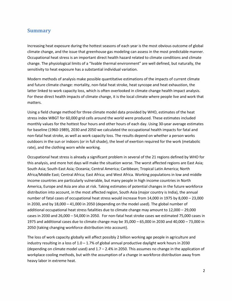
Summary

Increasing heat exposure during the hottest seasons of each year is the most obvious outcome of global

climate change, and the issue that greenhouse gas modeling can assess in the most predictable manner.

Occupational heat stress is an important direct health hazard related to climate conditions and climate

change. The physiological limits of a “livable thermal environment” are well defined, but naturally, the

sensitivity to heat exposure has a substantial individual variation.

Modern methods of analysis make possible quantitative estimations of the impacts of current climate

and future climate change: mortality, non-fatal heat stroke, heat syncope and heat exhaustion, the

latter linked to work capacity loss, which is often overlooked in climate change health impact analysis.

For these direct health impacts of climate change, it is the local climate where people live and work that

matters.

Using a field change method for three climate model data provided by WHO, estimates of the heat

stress index WBGT for 60,000 grid cells around the world were produced. These estimates included

monthly values for the hottest four hours and other hours of each day. Using 30-year average estimates

for baseline (1960-1989), 2030 and 2050 we calculated the occupational health impacts for fatal and

non-fatal heat stroke, as well as work capacity loss. The results depend on whether a person works

outdoors in the sun or indoors (or in full shade), the level of exertion required for the work (metabolic

rate), and the clothing worn while working.

Occupational heat stress is already a significant problem in several of the 21 regions defined by WHO for

this analysis, and more hot days will make the situation worse. The worst affected regions are East Asia;

South Asia; South-East Asia; Oceania; Central America; Caribbean; Tropical Latin America; North

Africa/Middle East; Central Africa; East Africa; and West Africa. Working populations in low and middle

income countries are particularly vulnerable, but many people in high income countries in North

America, Europe and Asia are also at risk. Taking estimates of potential changes in the future workforce

distribution into account, in the most affected region, South Asia (major country is India), the annual

number of fatal cases of occupational heat stress would increase from 14,000 in 1975 by 8,000 – 23,000

in 2030, and by 18,000 – 41,000 in 2050 (depending on the model used). The global number of

additional occupational heat stress fatalities due to climate change may amount to 12,000 – 29,000

cases in 2030 and 26,000 – 54,000 in 2050. For non-fatal heat stroke cases we estimated 75,000 cases in

1975 and additional cases due to climate change may be 35,000 – 65,000 in 2030 and 40,000 – 73,000 in

2050 (taking changing workforce distribution into account).

The loss of work capacity globally will affect possibly 2 billion working age people in agriculture and

industry resulting in a loss of 1.0 – 1.7% of global annual productive daylight work hours in 2030

(depending on climate model used) and 1.7 – 2.4% in 2050. This assumes no change in the application of

workplace cooling methods, but with the assumption of a change in workforce distribution away from

heavy labor in extreme heat.

3

If these work hour losses create equivalent reductions of global GDP, which has been estimated at 140

trillion US dollars in 2030, the global costs of increased occupational heat stress would be 1.4 – 2.4

trillion US dollars in 2030. In the worst affected regions (South Asia and West Africa) the estimated

annual work capacity losses at population level are at least twice as high. The worst affected people are

those working outdoors in the sun in heavy labor jobs. They already lose approximately 10% of annual

daylight work hours due to extreme heat in the hottest regions and this may increase to beyond 20% in

2050. People working in light jobs indoors are not so much affected, and air conditioning can of course

prevent the high workplace heat exposures at high cost in certain occupations and countries. Many

outdoor jobs, and jobs in workshops and factories, in low and middle income countries are paid at low

rates and not likely to receive the protective benefit of air conditioning.

The access to cooling systems for hundreds of millions of people is highly questionable as a recent

estimate of the number of people lacking basic sanitation in 2050 was 1.4 billion people. Will they

benefit from occupational heat stress prevention at work; - most likely not. Our analysis highlights the

major negative impacts that climate change will have on millions of working people. More precise

analysis is needed to quantify the costs and benefits of different adaptation and mitigation policies and

programs in different countries.

A summary of quantitative estimates for 2030 implies:

Grid cell based analysis of climate change shows increased heat and longer heat periods

particularly in tropical and sub-tropical areas

There may be 22,000 more occupational heat stroke fatalities in 2030 than in 1975; to this

should be added many thousand cases of non-fatal heat strokes and other clinical effects

Productive annual daylight work hours will be lost globally at 1.4% in 2030, and the global

economic costs of the lost labor productivity may be 2 trillion USD per year. The losses at

country level will be at multi-billion dollar level for many low and middle income countries.

The “work life years” lost (similar notion as DALYs) due to occupational heat stroke fatalities in

2030 will be approximately 880,000, while the “work life years” lost due to labor productivity

loss may be 70 million years, indicating that the labor productivity loss could be 70 times more

damaging to healthy, productive and disability-free life years than the fatalities.

For a country that will lose an estimated 100 billion USD per year in 2030 due to climate change

related increasing heat exposures, it may be a good investment to spend 1 million USD on

research and analysis to develop policies and programs to reduce the economic impacts of

occupational heat stress. Even if the cost estimate (100 billion USD) is 10 times too high, and the

research and analysis only reduces the actual cost by 10%, the savings could still be 1 billion USD

per year.

4

Background

Occupational heat stress as a global health risk

The modelling of global climate change uses greenhouse gas emission estimates and resulting

atmospheric heating as a key input into the global assessments (IPCC, 2013, WG1). Clearly, the

atmospheric temperature is a primary modelling result and therefore any health and social effects of

changing air temperatures are more directly assessed than most of the other projected changes of the

climate (humidity, wind, rainfall, etc.). The details of these occupational health and social effects are

described in a more detailed report (Kjellstrom et al., 2014a), while this paper summarizes the methods

and selected results.

The direct health impacts of heat exposure are generally analysed principally in terms of mortality or

hospital admissions (Kovats and Hajat, 2008). Elderly people are at the highest risk for these effects.

However, the risk of heat stroke amongst younger working people is well known and explained by the

limits of human physiological acclimatization (Parsons, 2003; a new edition of this textbook was

published in 2014). Significant numbers of working people die due to heat stroke even in high income

countries, as described in a recent study of agricultural workers in the USA (MMWR, 2008). It is also of

interest that more than one thousand additional deaths occurred in the age range 15-64 years during

the two weeks of extreme heat wave in France in August 2003 (Hemon and Jougla, 2003), but no

analysis of the workplace heat exposure contribution to this increased mortality has been carried out.

Apart from clinical health effects, work capacity is affected by excessive heat exposure and hourly work

output is reduced (Bridger, 2003; Kjellstrom, et al., 2009a). These impacts on working people have been

generally ignored in international reviews of climate change effects (e.g. Costello et al., 2009), which is

partly a symptom of the low priority given to occupational health, the focus on “diseases”, and the belief

that adult humans can adapt to the emerging heat conditions.

Local people in any part of the world need to adapt as best they can to heat and cold exposure by

cultural practices such as “siesta” during the hottest part of the day, reduced work intensity, and the use

of hats outdoors and other appropriate clothing (Parsons, 2009). The performance of necessary work

during the cooler night hours is an option in some situations, but many work tasks depend on daylight

and with climate change even the coolest night hours may create heat stress because humidity can

increase to near 100% at night. Traditional practices to reduce heat exposure (e.g. siesta) may be

labelled “behavioural acclimatisation” as a part of “adaptation” (Ebi and Semenza, 2008; Fussel et al.,

2006) as the preventive effects complement the benefits of “physiological acclimatisation”. The

problem is that the hotter it gets, the longer siesta is needed.

As little as 20% of muscle energy contributes to external “work” (Parsons, 2014), and the rest becomes

“waste heat” inside the body that needs to be released to the external environment. At high air

temperatures (above 34-37 oC), the only method of heat loss to counteract bodily heat gain caused by

work, is via evaporation of sweat. When there is high humidity, sweat evaporation is insufficient and

5

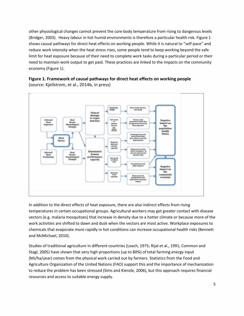
other physiological changes cannot prevent the core body temperature from rising to dangerous levels

(Bridger, 2003). Heavy labour in hot humid environments is therefore a particular health risk. Figure 1

shows causal pathways for direct heat effects on working people. While it is natural to “self-pace” and

reduce work intensity when the heat stress rises, some people tend to keep working beyond the safe

limit for heat exposure because of their need to complete work tasks during a particular period or their

need to maintain work output to get paid. These practices are linked to the impacts on the community

economy (Figure 1).

Figure 1. Framework of causal pathways for direct heat effects on working people (source: Kjellstrom, et al., 2014b, in press)

In addition to the direct effects of heat exposure, there are also indirect effects from rising

temperatures in certain occupational groups. Agricultural workers may get greater contact with disease

vectors (e.g. malaria mosquitoes) that increase in density due to a hotter climate or because more of the

work activities are shifted to dawn and dusk when the vectors are most active. Workplace exposures to

chemicals that evaporate more rapidly in hot conditions can increase occupational health risks (Bennett

and McMichael, 2010).

Studies of traditional agriculture in different countries (Leach, 1975; Rijal et al., 1991; Common and

Stagl, 2005) have shown that very high proportions (up to 80%) of total farming energy input

(MJ/ha/year) comes from the physical work carried out by farmers. Statistics from the Food and

Agriculture Organization of the United Nations (FAO) support this and the importance of mechanization

to reduce the problem has been stressed (Sims and Kienzle, 2006), but this approach requires financial

resources and access to suitable energy supply.

6

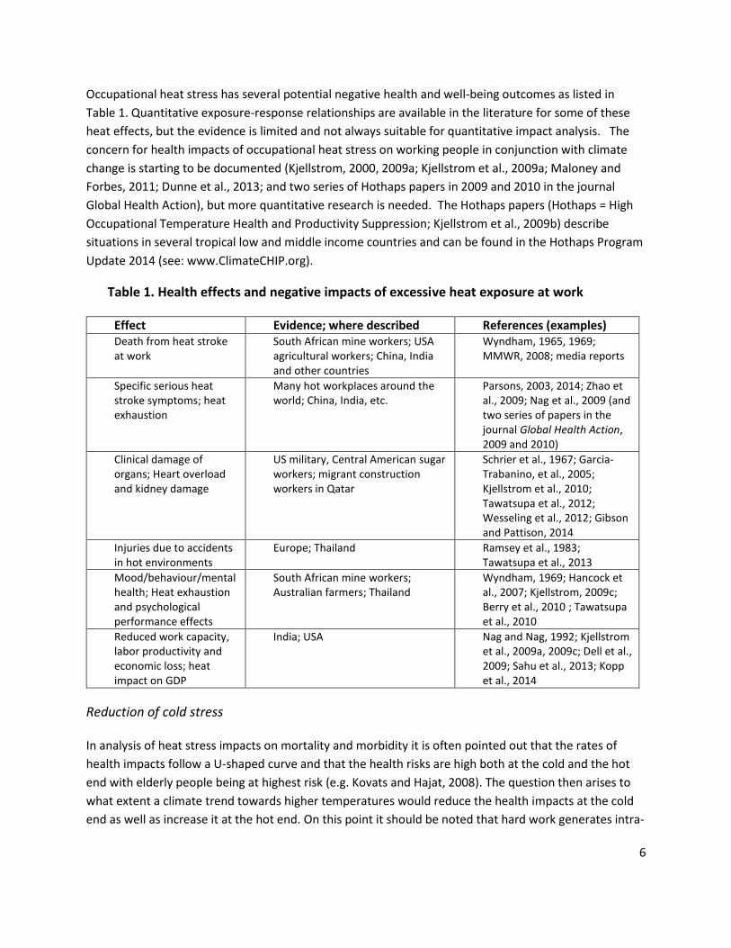
Occupational heat stress has several potential negative health and well-being outcomes as listed in

Table 1. Quantitative exposure-response relationships are available in the literature for some of these

heat effects, but the evidence is limited and not always suitable for quantitative impact analysis. The

concern for health impacts of occupational heat stress on working people in conjunction with climate

change is starting to be documented (Kjellstrom, 2000, 2009a; Kjellstrom et al., 2009a; Maloney and

Forbes, 2011; Dunne et al., 2013; and two series of Hothaps papers in 2009 and 2010 in the journal

Global Health Action), but more quantitative research is needed. The Hothaps papers (Hothaps = High

Occupational Temperature Health and Productivity Suppression; Kjellstrom et al., 2009b) describe

situations in several tropical low and middle income countries and can be found in the Hothaps Program

Update 2014 (see: www.ClimateCHIP.org).

Table 1. Health effects and negative impacts of excessive heat exposure at work

Effect Evidence; where described References (examples) Death from heat stroke at work

South African mine workers; USA agricultural workers; China, India and other countries

Wyndham, 1965, 1969; MMWR, 2008; media reports

Specific serious heat stroke symptoms; heat exhaustion

Many hot workplaces around the world; China, India, etc.

Parsons, 2003, 2014; Zhao et al., 2009; Nag et al., 2009 (and two series of papers in the journal Global Health Action, 2009 and 2010)

Clinical damage of organs; Heart overload and kidney damage

US military, Central American sugar workers; migrant construction workers in Qatar

Schrier et al., 1967; Garcia-Trabanino, et al., 2005; Kjellstrom et al., 2010; Tawatsupa et al., 2012; Wesseling et al., 2012; Gibson and Pattison, 2014

Injuries due to accidents in hot environments

Europe; Thailand Ramsey et al., 1983; Tawatsupa et al., 2013

Mood/behaviour/mental health; Heat exhaustion and psychological performance effects

South African mine workers; Australian farmers; Thailand

Wyndham, 1969; Hancock et al., 2007; Kjellstrom, 2009c; Berry et al., 2010 ; Tawatsupa et al., 2010

Reduced work capacity, labor productivity and economic loss; heat impact on GDP

India; USA Nag and Nag, 1992; Kjellstrom et al., 2009a, 2009c; Dell et al., 2009; Sahu et al., 2013; Kopp et al., 2014

Reduction of cold stress

In analysis of heat stress impacts on mortality and morbidity it is often pointed out that the rates of

health impacts follow a U-shaped curve and that the health risks are high both at the cold and the hot

end with elderly people being at highest risk (e.g. Kovats and Hajat, 2008). The question then arises to

what extent a climate trend towards higher temperatures would reduce the health impacts at the cold

end as well as increase it at the hot end. On this point it should be noted that hard work generates intra-

7

body heat so it is of benefit in colder climates and a significant disadvantage in hotter climates. This

must be considered when analyzing the impact of climate change on working people rather than on

sedentary elderly people.

A factor of importance for heat and cold exposure is the distribution of the global population by latitude.

In 2000 approximately 3,400 million people lived in the tropical and sub-tropical areas (30 degrees up

and down from the equator), where additional heat is a hazard, while only 1.9 million people lived in the

arctic area with extreme cold (beyond 66 degrees from equator) (based on UN population data). Few

people live at high altitude where extreme cold can also be a hazard. In the highly populated warmer

areas significant morbidity or work capacity loss due to cold is not to be expected (Parsons, 2014).

Relevant previous studies and estimates A key issue in the analysis of climate impacts on occupational health and safety is the extent to which

the daily “heat stress” or “heat load” will increase. Global gridded estimates of current and future “heat

load” have been published by Jendritzky and Tinz (2009), including maps of a heat stress index used in

Germany: the HeRATE index (Health Related Assessment of the Thermal Environment). This index takes

into account “heat and cold comfort” based on common clothing use in different climates, and local

acclimatization over preceding weeks. The published maps included background estimates for 1971 –

1980 and future estimates for 2041 – 2050, and show that increased heat stress is likely in most parts of

the world. Another global gridded analysis, using Tw (here = Tpwb) (psychrometric wet bulb

temperature) as an indicator of human heat stress (Sherwood and Huber, 2010), concluded that global

climate change could substantially reduce habitability of some regions.

The impacts on health and work capacity (and productivity) at an individual level have been studied and

published by physiologists and ergonomists for several decades (see reviews by Parsons, 2014 and

Bridger, 2003), but analysis in relation to climate change is rare. An analysis for Perth, Australia

(Maloney and Forbes, 2011) showed the likely physiological effect of heat exposure and physical activity

intensity (including work) on human performance capacity in Perth in the current climate conditions and

how it may change in the future based on projections of Australia’s climate until 2070. It was calculated

(Maloney and Forbes, 2011) that an average person acclimatized to heat could safely carry out physical

activity or manual labour outdoors in the daytime during all but one day per year in the 1990s. However,

climate change would increase the number of days with dangerous daytime heat exposure to 15-26 days

per year in the 2070s. It should be pointed out that Perth is not a place with the most extremely

physiologically challenging heat as high temperatures often occur with concurrent low humidity.

The first quantitative estimates of the impacts of workplace heat on populations in relation to climate

change were included as tentative analysis in a conference presentation by Kjellstrom (2000). Another

analysis by Kjellstrom et al., (2009c) was the first attempt to assess regional and global impacts of

climate change on workplace heat exposures and on productivity. The climate and heat stress data were

estimated for a few "representative" locations within 21 large global regions (the same regions as the

8

ones used in this report). The results (Kjellstrom et al., 2009c) showed that climate change until 2050

would reduce the available work hours in all regions (compared to 1961-1990 as a baseline; in this

report labeled “1975”), assuming the mixture of jobs outdoors/indoors and at different work intensities

stayed the same. The estimated reductions varied between 0.2 % for Australasia and 18.2 % for South

East Asia and 18.6 % for Central America. Apart from these two regions, the other most affected regions

were West Africa (15.8% reduction), Central Africa (15.4%), Oceania (15.2%), Caribbean (11.7%) and

South Asia (11.5%).

When assumptions about changing workforce distributions due to increasing GDP (from baseline “1975”

to 2050) were included (Kjellstrom et al., 2009c), the reductions of available work hours were more

limited as it was assumed that fewer people will be working in highly heat exposed heavy physical labor

jobs in the 2050s. Two regions had estimated population average work capacity increasing somewhat

until 2050 due to such assumed workforce changes (tropical Latin America and Southern Africa) and two

had no change (West Europe and Central Europe), but in all the other 17 regions the estimated

reduction of work capacity by 2050 would be between 0.1 and 4.4%, except for the Caribbean region

and Central America where particularly high reductions at 7.7 and 18.6%, respectively, were calculated

(Kjellstrom et al., 2009c). These results will be compared with our new estimates in the Discussion

section.

Additional analysis of the impacts of workplace heat on working people was published by Dunne et al

(2013). They focused on the labor productivity loss during the hottest months in each part of the world

and compared estimated WBGT levels with the US national (ACGIH, 2009) and international (ISO, 1989)

standards. Very large reductions of “labor capacity” due to heat have already taken place (as high as

90%) and further major reductions are projected (Dunne et al., 2013). As we will show below, using the

workplace standards create larger calculated reductions than the likely reductions for a typical

workforce. Another analysis of labor productivity loss for the USA (Kopp et al., 2014) was based on a

single study of time use patterns in the USA in relation to daily heat conditions. It showed reduced time

use during the hottest months in most of the USA and the results were presented as economic losses.

These issues will be analyzed in the Discussion.

In conclusion, the few published studies with an analysis of heat exposure impacts on human capacity

for physical activities at work (or during “active transport” or leisure or just carrying out routine daily

tasks) indicate that substantial losses may occur in areas with hot seasons.

Description of models

Conceptual basis

There are four calculation models for this assessment. Three of the models are deterministic as they use

physics principles and biological mechanisms for heat effects on working people, and descriptive studies

9

of susceptibility as the foundation for impact calculations. These three models cover [Model 1]

occupational heat stress exposure, [Model 2] exposure-response relationships for clinical health risks,

and [Model 3] such relationships for suppression of labor productivity (or work capacity). The fourth

model [Model 4] relates country level average GDP to the percentage of the country’s workforce in

agriculture, industry and services, and is based on statistical records. This model deals with “structural

change” of economies. The associated longer report (Kjellstrom et al., 2014a) will provide additional

detail about each model and the input data used.

Climate variables of importance to human heat exposure

Four climate variables influence the relevant human heat exposure quantification whether it is at

“baseline”, current situation, or at future time points: air temperature, humidity, air movement (wind

speed) and heat radiation (outdoors mainly from the sun) (Parsons, 2014). Daily solar heat radiation is

difficult to model because of variable cloud cover and the unavailability of future heat radiation values

for each grid cell in our analysis. Estimates with no solar heat radiation would represent the exposure

situation indoors (without a local heat source) or in full shade outdoors. Wind speed can vary

significantly during the course of a day and an average daily wind speed is not useful to determine the

WBGT during the hottest time of the day when wind speed may be low. Also, working persons usually

move their arms and legs generating their own air movement over their skin (at approximately 1 m/s).

Because of these uncertainties we have chosen to calculate heat exposure indoors (or in full shade)

where there is no solar radiation and wind speed is likely to be more constant (it can be increased by

fans, but when air temperature is above 37 oC and humidity is high, fans may actually increase the heat

stress). The outdoor heat exposure is then estimated from the indoor values based on the expected

additional exposure in full sun during the middle of the day. The wind impact on WBGT is limited when

the wind speed exceeds 1 m/s, especially when the wind is warm (Lemke and Kjellstrom, 2012).

Heat stress depends on two additional factors (Parsons, 2014): the metabolic rate (a function of physical

work intensity) and the type of clothing worn (which influences the evaporation of sweat and direct heat

radiation on the body). Much detailed research has dealt with the design of clothing or the clothing

materials that serve as a barrier against heat. The physiological basis for these relationships between the

environment, behaviors and modifiers is well known (Bridger, 2003), and it has been taken into account

when international standards were developed for heat stress (e.g. ISO, 1989; Parsons, 2014). We

assume that people working in hot conditions are using light clothing. If they use chemical protection

clothing the heat stress will increase. If the heat stress exceeds the individual limits of physiological

defense mechanisms, symptoms and signs of heat strain will develop as steps towards the more serious

clinical health effects listed in Table 1.

We use WBGT (Wet Bulb Globe Temperature) as the key indicator of occupational heat exposure as it is

the most common human heat exposure index used in situations of occupational heat stress (Yaglou and

Minard, 1957; Parsons, 2014). It is the parameter used in the international standard for occupational

heat exposure (ISO, 1989), in the recommendations from the American Conference of Governmental

Industrial Hygienists (ACGIH, 2009), and in guidelines or regulations from government departments in a

10

number of countries (e.g. New Zealand: DoLNZ, 1997). The recently developed Universal Thermal

Climate Index (UTCI; see website www.utci.org) is based on advanced physiological modeling (Fiala et

al., 2011), but it is not designed for population health research or occupational heat stress estimations.

Model 1: Quantifying human occupational heat stress exposure

Calculation of WBGT from routine climate data

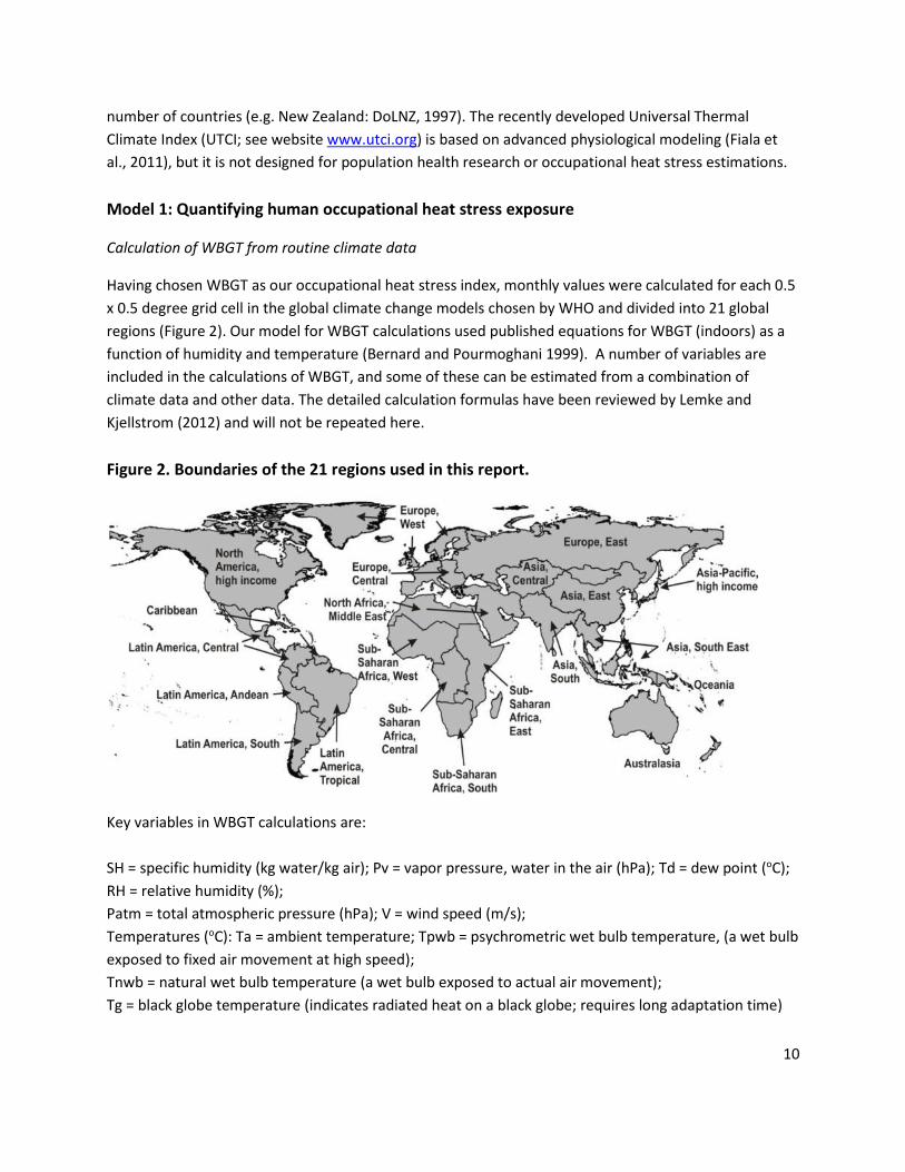
Having chosen WBGT as our occupational heat stress index, monthly values were calculated for each 0.5

x 0.5 degree grid cell in the global climate change models chosen by WHO and divided into 21 global

regions (Figure 2). Our model for WBGT calculations used published equations for WBGT (indoors) as a

function of humidity and temperature (Bernard and Pourmoghani 1999). A number of variables are

included in the calculations of WBGT, and some of these can be estimated from a combination of

climate data and other data. The detailed calculation formulas have been reviewed by Lemke and

Kjellstrom (2012) and will not be repeated here.

Figure 2. Boundaries of the 21 regions used in this report.

Key variables in WBGT calculations are:

SH = specific humidity (kg water/kg air); Pv = vapor pressure, water in the air (hPa); Td = dew point (oC);

RH = relative humidity (%);

Patm = total atmospheric pressure (hPa); V = wind speed (m/s);

Temperatures (oC): Ta = ambient temperature; Tpwb = psychrometric wet bulb temperature, (a wet bulb

exposed to fixed air movement at high speed);

Tnwb = natural wet bulb temperature (a wet bulb exposed to actual air movement);

Tg = black globe temperature (indicates radiated heat on a black globe; requires long adaptation time)

11

The calculations produce valid estimates of “in shade” (or indoor) WBGT using input formulas from

Bernard and Pourmoghani (1999) and Brice and Hall (2009). Direct calculation of WBGT outdoors

requires solar radiation data that is not normally available in climate modeling or from weather stations.

WBGT outdoor calculation formulas have been published by Liljegren et al. (2008) and Gaspar and

Quintela (2009), but they require daily heat radiation data. The method for “in sun” WBGT (outdoors)

has been described in Lemke et al., (2011) and Lemke and Kjellstrom (2012).

Studies for selected locations using hourly climate data for 1999 (ISH GSOD data from: NOAA, 2009)

showed the increase in WBGT when heat exposure from the solar radiation is included: the difference

between “in sun” and “in shade” WBGT (solar radiation, SR > 600 W/m2) can be approximated to 3 oC

(rounded value to single degree) during the hottest and sunniest part of the day (Kjellstrom et al.,

2014a). A common heat radiation inflow in the full sun on afternoons in tropical and other hot locations

is 600 W/m2. We chose the decile 7.5 value (2.91 3 oC rounded) because the maximum effect of the

sun is expected during the hottest 2-4 hours each day (approximately 25% of daylight hours).

Hourly variations in WBGT levels

For the work capacity loss calculations we need to estimate the hourly WBGT levels, as the effects are

acute and apply to each working hour (Parsons, 2014). In order to assess the relationship between

routinely recorded climate variables, such as maximum and mean daily temperature and mean daily

dew point, we used hourly data from NOAA/GSOD and compared calculations of indoor WBGT using

daily and hourly data at a number of locations with very hot periods. We divided the daylight hours into

three 4-hour time periods: The hottest part of the day between 12-15:59 where the WBGT = WBGTmax.

The surrounding 2-hour periods (10.00 – 11.59 and 16.00 – 17.59 Hours) where the WBGT = WBGThalf =

(WBGTmax + WBGTmean)/2 and the next surrounding 2 hour periods (08.00 – 09.59 and 18.00 – 19.59

hours) where WBGT = WBGTmean (for the 24 hour period). Thus, we decided to use these three WBGT

levels during typical working days as our indicators of hourly heat stress levels. The estimates are not

exact, but we consider them a reasonable approximation of the actual hourly WBGT levels indoors or in

full shade outdoors.

Process used for quantifying heat exposure in global grid cells

General Circulation Models (GCM) used to calculate climate change often produce outputs on

approximately 3 -degree grid cell size, though this varies from model to model. These large cells (300 km

square at the equator) do not align well with the 21 regions defined by WHO for this project (Figure 2)

and are much too large to attribute to specific locations. Half degree grid cell data (50 km square at the

equator) was supplied by the WHO team. While 50 km grid cells derived from 300 km grid cells do not

have more information than what is available from the 300 km grid cells, they do allow proportions of

the larger grid cells to be assigned to the correct regions. This process of taking 300 km grid cells,

downsizing to 50km grid cells (using bilinear interpolation) and then allocating the 50 km grid cells into

regions leads to some inaccuracies, particularly in regions with variable topography (e.g. South Asia,

Andean Latin America, West Europe) where substantial parts of the 300 km grid cell is at higher (colder)

12

altitude than other parts. However, these errors are not likely to cause major errors in the heat stress

calculations because the affected areas are colder than the thresholds for effects.

Suitable 0.5 x 0.5 degree gridded modeled data was supplied for 3 GCM models: BCM2, IPCM4, and

EGMAM. The model results had been produced for WHO by CRU in the United Kingdom (Goodess and

Harris, 2010) and will not be described in detail here. The results of the EGMAM model were supplied

for three separate runs: EGMAM1, EGMAM2 and EGMAM3. We decided to use their average as one

model, because the difference between the results of the three runs was minor.

BCM = Bergen Climate Model (from Bergen University, Norway)

EGMAM = ECHO-G2 with Middle Atmosphere and Messy interface climate model (from Free University

Berlin, Germany)

IPCM = Institute Pierre Simone Laplace – Climate Model (from Institute PSL, France)

We obtained the monthly actual climate data for every year in the period 1961 to 2002 for 0.5 x 0.5

degree (50km square at the equator) grid cells from the University of East Anglia Climate Research Unit

(CRU, 2004; Mitchell & Jones 2005). We averaged the data (monthly water vapour pressure, maximum

temperature, mean temperature) for the period 1961-1990 to get a single “1975” baseline value for

each grid cell. The annual averages and standard deviations (and coefficients of variation, CVs) of the

WBGTmax data for grid cells in each region were used to estimate the likely uncertainties in our results

(Kjellstrom et al, 2014a). The CVs were generally in the range 2-5% of the average WBGTmax values,

which indicates that the actual region-based values would not deviate more than 10% from our

calculated estimates in the following analysis (see “Uncertainty” section in this report).

Computation method

The climate and population data for the grid cells (approximately 60,000 cells with land areas in the cell)

were imported into Excel and then subjected to a number of quality control checks: a check for

consistency of latitude/longitude, a check to ensure the year and the months matched and were

consecutive, and a check to see if the various maps were keyed together.

The monthly grid cell data for the 30-year periods around 1975, 2030 and 2050 was processed to

determine the following:

Monthly averages of daily mean and maximum air temperatures. --- These temperatures (Ta)

varied during the day and the calculation process described above captured this variation.

Monthly averages of dew point (Td) from the water vapor pressure (or specific humidity) and

the mean air temperature; the absolute humidity (indicated by Td), which is relatively stable

during most days, was assumed to be constant throughout each 24-hour period.

13

Psychrometric wet bulb temperature (Tpwb) calculated from the dew point and temperature

with standard physics formulas.

WBGT (“in shade” or indoor) calculated from the psychrometric wet bulb temperature and air

temperature. --- The three levels were calculated: WBGTmax, WBGThalf, and WBGTmean. Air

movement over the skin (wind speed) was set at 1 m/s and clothing was assumed to be light.

The distributions for each region of the number of “grid-cell-months” per year at each WBGT

(“in shade”) one degree level for max, half and mean. These distributions show the changing

heat exposure situation between the three time periods in each grid cell. The combined monthly

data for the grid cells in each region provided a distribution of heat exposures in the full region.

The WBGT (“in sun”) levels during the four hottest hours were assessed by adding 3 oC to the

WBGTmax levels (in shade) for each month. Clearly the percentage cloud cover and variation in

cloud cover during each day will influence the resulting hourly WBGT outdoors levels. The

WBGThalf and WBGTmean levels were kept at the “in shade” levels because the sun heat

radiation is less intense at these hours and we did not want to over-estimate the daily averages.

The population-based heat exposure was calculated as annual person-months of exposure for

clinical health effects and annual person-hours of exposure for work capacity loss analysis at

each 1 oC WBGT step for each of the 21 WHO regions. This uses the grid cell based WBGT values

and population sizes in each of the three 30-year time periods.

Calculating person-time exposure variables

In order to calculate risks per million working people per year, we developed person-time exposure

variables. The climate and WBGT estimates are for monthly time blocks, so we assume 20 working days

per month (a conservative estimate, some people work every day) and that the monthly WBGT values

apply to each working day of that month. Thus, the exposure variables are person-days of exposure

based on person-months of exposure (and the 20 working days per month). When estimating work

capacity loss we also use person-hours of exposure, taking estimated daily variation in heat exposure

into account. Our exposure estimates are “conservative” in the sense that half of the days each month

would have exposure levels higher than the average, and the days with the highest heat levels create

the greatest impacts (the exposure-response relationships are not linear).

For each time period (baseline “1975”, “2030” and “2050”) tables of the annual person-months of

exposure in each of the 21 regions at each WBGT 1 oC level were calculated from the monthly grid cell

estimates. The exposure-response relationships indicate that effects start occurring in working people

carrying out intensive labor at WBGT = 26 oC. We start these person-month calculations at monthly

average WBGTs at 23 oC as this gives us a chance to analyse the impact of region-wide changes in the

WBGT values and we can also estimate afternoon outdoor heat exposures in the sun ( + 3 oC). Expressing

the population average heat exposures in this manner makes it possible to calculate impacts per million

people in specific geographic areas.

14

Model 2: Clinical health effects and exposure-response relationships

Health effects chosen

The clinical health effects included here are acute and related to the maximum heat exposure levels

(WBGTmax) on a particular day, but the published exposure-response relationships for fatal and non-

fatal heat stroke are annual incidence rates for people in mines with relatively continuous exposures

(see the section on exposure-response relationships). The relationships for seasonally varying heat

exposure levels are not known, so we calculated person-months of exposure at each WBGTmax level and

applied 1/12 of the published annual risk to these monthly exposure estimates.

In calculations of heat exhaustion as a clinical effect, we can also assume that the risk relates to the

highest exposure on each day. Thus the monthly average WBGTmax is used for each month and the

exposure variable is the number of person-days of exposure at WBGTmax per year (assuming each

working day in a particular month had the same level as the monthly average).

Published exposure-response relationships

The scientific evidence behind quantitative exposure-response relationships for clinical health effects

and work capacity impacts of hot work environments is incomplete and varies between studies. One

important problem is that published studies use different heat exposure variables. We assume that heat

exposure indexes expressed as oC are correlated. As discussed earlier, we have based our estimates of

heat exposures on WBGT, assuming that other heat stress indexes are approximately inter-changeable

with WBGT (after correction for different scales and ranges of values).

We assumed, because of lack of gender-specific data sufficient to quantify gender differences, that the

risks for women and men are the same (but this needs to be explored in future research). We also

assume that the risks in different age ranges within the working age groups are the same (e.g. 20- and

50-year olds are at the same risk). However, in addition to potential age and gender differences,

sensitivity to occupational heat exposure is likely to vary between societies. There are indications that

people who live their whole lives in a hot environment develop behavioural adaptation to avoid heat

impacts, and/or modify their physiological interaction with heat (Wakabayashi et al., 2010).

Wyndham (1965) and Wyndham (1969) report exposure-response relationships for serious health

impacts in black (“Bantu”) mine workers in South Africa; non-fatal and fatal heat stroke (Table 2). The

relationships are for acclimatized workers. For non-acclimatized workers the reported risks were higher,

but our analysis assumes that most of the working people in hot places are already acclimatized to the

local conditions. These South Africa data refer to underground mine workers, who worked in a hot

environment with relative humidity (RH) close to 100% (because water spray was used inside the hot

mine to reduce hazardous dust exposure). The calculated levels of effective temperature (ET) and WBGT

are very similar (Walters, 1968) and Tpwb, as well as Ta, are equal to WBGT when the RH is near 100%.

Thus, we consider the exposure-response relationships in Table 2 to be valid also for WBGT. These

relationships indicate curvilinear continuously increasing risks as heat exposure increases. Wyndham

15

(1969) reports heat exposure data as Tpwb, ET and WBGT in different publications. These heat exposure

variables are approximately equivalent at the very high humidity inside the mines (Wyndham reported

cases for the whole 6-year period, which we show as annual and monthly rates in Table 2).

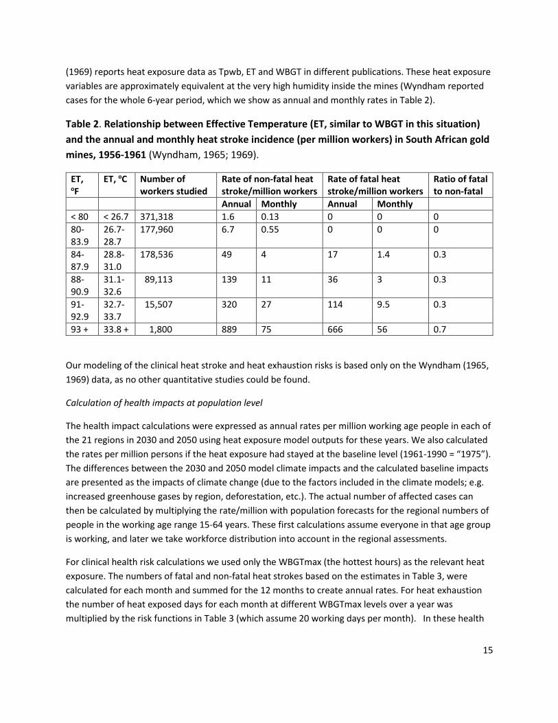
Table 2. Relationship between Effective Temperature (ET, similar to WBGT in this situation)

and the annual and monthly heat stroke incidence (per million workers) in South African gold

mines, 1956-1961 (Wyndham, 1965; 1969).

ET, oF

ET, oC Number of workers studied

Rate of non-fatal heat stroke/million workers

Rate of fatal heat stroke/million workers

Ratio of fatal to non-fatal

Annual Monthly Annual Monthly

< 80 < 26.7 371,318 1.6 0.13 0 0 0

80-83.9

26.7-28.7

177,960 6.7 0.55 0 0 0

84-87.9

28.8-31.0

178,536 49 4 17 1.4 0.3

88-90.9

31.1-32.6

89,113 139 11 36 3 0.3

91-92.9

32.7-33.7

15,507 320 27 114 9.5 0.3

93 + 33.8 + 1,800 889 75 666 56 0.7

Our modeling of the clinical heat stroke and heat exhaustion risks is based only on the Wyndham (1965,

1969) data, as no other quantitative studies could be found.

Calculation of health impacts at population level

The health impact calculations were expressed as annual rates per million working age people in each of

the 21 regions in 2030 and 2050 using heat exposure model outputs for these years. We also calculated

the rates per million persons if the heat exposure had stayed at the baseline level (1961-1990 = “1975”).

The differences between the 2030 and 2050 model climate impacts and the calculated baseline impacts

are presented as the impacts of climate change (due to the factors included in the climate models; e.g.

increased greenhouse gases by region, deforestation, etc.). The actual number of affected cases can

then be calculated by multiplying the rate/million with population forecasts for the regional numbers of

people in the working age range 15-64 years. These first calculations assume everyone in that age group

is working, and later we take workforce distribution into account in the regional assessments.

For clinical health risk calculations we used only the WBGTmax (the hottest hours) as the relevant heat

exposure. The numbers of fatal and non-fatal heat strokes based on the estimates in Table 3, were

calculated for each month and summed for the 12 months to create annual rates. For heat exhaustion

the number of heat exposed days for each month at different WBGTmax levels over a year was

multiplied by the risk functions in Table 3 (which assume 20 working days per month). In these health

16

risk calculations we also took into account work location (indoors or outdoors) and work intensity

(heavy, moderate or light).

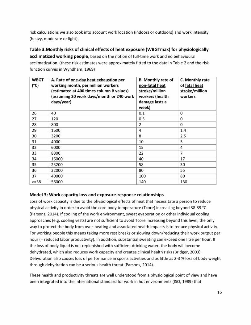
Table 3.Monthly risks of clinical effects of heat exposure (WBGTmax) for physiologically

acclimatized working people, based on the notion of full-time work and no behavioural

acclimatization. (these risk estimates were approximately fitted to the data in Table 2 and the risk

function curves in Wyndham, 1969)

WBGT (oC)

A. Rate of one-day heat exhaustion per working month, per million workers (estimated at 400 times column B values) (assuming 20 work days/month or 240 work days/year)

B. Monthly rate of non-fatal heat stroke/million workers (health damage lasts a week)

C. Monthly rate of fatal heat stroke/million workers

26 40 0.1 0

27 120 0.3 0

28 800 2 0

29 1600 4 1.4

30 3200 8 2.5

31 4000 10 3

32 6000 15 4

33 8800 22 7

34 16000 40 17

35 23200 58 30

36 32000 80 55

37 40000 100 80

>=38 56000 140 130

Model 3: Work capacity loss and exposure-response relationships

Loss of work capacity is due to the physiological effects of heat that necessitate a person to reduce

physical activity in order to avoid the core body temperature (Tcore) increasing beyond 38-39 oC

(Parsons, 2014). If cooling of the work environment, sweat evaporation or other individual cooling

approaches (e.g. cooling vests) are not sufficient to avoid Tcore increasing beyond this level, the only

way to protect the body from over-heating and associated health impacts is to reduce physical activity.

For working people this means taking more rest breaks or slowing down/reducing their work output per

hour (= reduced labor productivity). In addition, substantial sweating can exceed one litre per hour. If

the loss of body liquid is not replenished with sufficient drinking water, the body will become

dehydrated, which also reduces work capacity and creates clinical health risks (Bridger, 2003).

Dehydration also causes loss of performance in sports activities and as little as 2-3 % loss of body weight

through dehydration can be a serious health threat (Parsons, 2014).

These health and productivity threats are well understood from a physiological point of view and have

been integrated into the international standard for work in hot environments (ISO, 1989) that

17

recommends limits of hourly work at different WBGT heat exposure levels and different work

intensities. Adjustments for different types of clothing are also included in the standard as heavy or

protective clothing increases the heat stress on the body. The standard aims to protect the majority of

workers by keeping their Tcore below 38 oC. The “majority” protection implies that it recommends more

rest time than is required by an average worker and for many individuals. National standards, such as

ACGIH (2009) for the USA, are based on similar concepts.

The effects of heat on work capacity occur during each hour of work if there is excessive heat exposure.

To calculate the equivalent total number of work hours lost, the number of hours at each level of WBGT

exposure for each person is required. The three WBGT values were used to approximately calculate

WBGT exposure: WBGTmax, WBGThalf and WBGTmean (four hours each) as indicated above. Thus, the

variable person-hours of exposure at a certain WBGT level is the sum of the hours in a month at the

three WBGT levels (four daylight hours of exposure at each WBGT level). Impacts on work during night

time hours have not been assessed in this study.

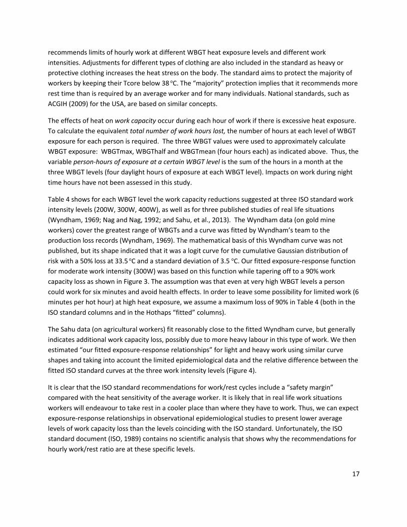
Table 4 shows for each WBGT level the work capacity reductions suggested at three ISO standard work

intensity levels (200W, 300W, 400W), as well as for three published studies of real life situations

(Wyndham, 1969; Nag and Nag, 1992; and Sahu, et al., 2013). The Wyndham data (on gold mine

workers) cover the greatest range of WBGTs and a curve was fitted by Wyndham’s team to the

production loss records (Wyndham, 1969). The mathematical basis of this Wyndham curve was not

published, but its shape indicated that it was a logit curve for the cumulative Gaussian distribution of

risk with a 50% loss at 33.5 oC and a standard deviation of 3.5 oC. Our fitted exposure-response function

for moderate work intensity (300W) was based on this function while tapering off to a 90% work

capacity loss as shown in Figure 3. The assumption was that even at very high WBGT levels a person

could work for six minutes and avoid health effects. In order to leave some possibility for limited work (6

minutes per hot hour) at high heat exposure, we assume a maximum loss of 90% in Table 4 (both in the

ISO standard columns and in the Hothaps “fitted” columns).

The Sahu data (on agricultural workers) fit reasonably close to the fitted Wyndham curve, but generally

indicates additional work capacity loss, possibly due to more heavy labour in this type of work. We then

estimated “our fitted exposure-response relationships” for light and heavy work using similar curve

shapes and taking into account the limited epidemiological data and the relative difference between the

fitted ISO standard curves at the three work intensity levels (Figure 4).

It is clear that the ISO standard recommendations for work/rest cycles include a “safety margin”

compared with the heat sensitivity of the average worker. It is likely that in real life work situations

workers will endeavour to take rest in a cooler place than where they have to work. Thus, we can expect

exposure-response relationships in observational epidemiological studies to present lower average

levels of work capacity loss than the levels coinciding with the ISO standard. Unfortunately, the ISO

standard document (ISO, 1989) contains no scientific analysis that shows why the recommendations for

hourly work/rest ratio are at these specific levels.

18

Table 4. Reduction of hourly work capacity at different levels of work intensity and heat

exposure (% reduction from background in cooler environment; acclimatized workers).

Sources ISO ISO

ISO Wyndham, 1969

Nag, 1992

Sahu, et al., 2013

Hothaps fitted

Hothaps fitted

Hothaps fitted

Our fitted exposure-response relationships

Labor intensity

Light, 200W

Moderate, 300W

Heavy, 400W

Moderate Light Moderate-heavy

Light Moderate Heavy

WBGT, ET or Tw

26 0 0 0 0 0 0 0 0 0

27 0 0 18 2 6 0 0 9

28 0 0 35 5 11 12 0 3 17

29 0 28 50 8 18 0 9 25

30 9 49 65 15 25 3 17 35

31 30 70 78 22 32 9 25 45

32 50 85 90 32 22 40 17 35 55

33 70 90 90 42 25 45 64

34 80 90 90 35 55 74

35 85 90 90 60 45 64 81

36 90 90 90 40 60 74 85

37 90 90 90 74 81 88

38 and above 90 90 90 86 88 90

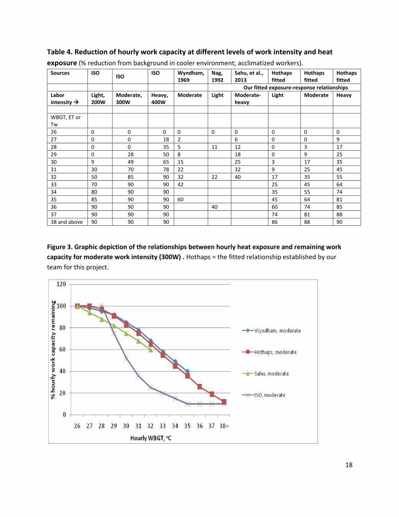
Figure 3. Graphic depiction of the relationships between hourly heat exposure and remaining work

capacity for moderate work intensity (300W) . Hothaps = the fitted relationship established by our

team for this project.

19

The ISO curve (Figure 3) has a different shape from the others because this is designed to protect most

workers where the other results relate to the average worker. In a population of workers, some are

very vulnerable to heat strain. At low heat stress all workers can cope with the conditions. As the heat

stress increases the impact on the more vulnerable workers is more pronounced so standards that

protect those workers must indicate lower work capacity. If the ISO (1989) standard (or the similar

ACGIH, 2009, standard) is used to calculate work capacity loss (as was done by Kjellstrom et al, 2009c,

and Dunne et al, 2013) the resulting values will be lower than if an average Hothaps relationship is used.

The calculation of work capacity loss each month for each grid cell follows similar calculation processes

as for clinical health effects described above. For each cell there can be six impact models (Table 4). In

this WHO report we only calculate the impacts on “average workers” using our fitted exposure-response

relationships. We calculate for indoor and outdoor exposures the percentage of daylight work hours

lost, assuming 12 potential daylight work hours per day and 20 work days per month (equivalent to 2880

hours per year). Taking holidays and other non-working days and hours into account, the usual annual

work hours in other reports has been assumed to be 2000 hours in high income countries.

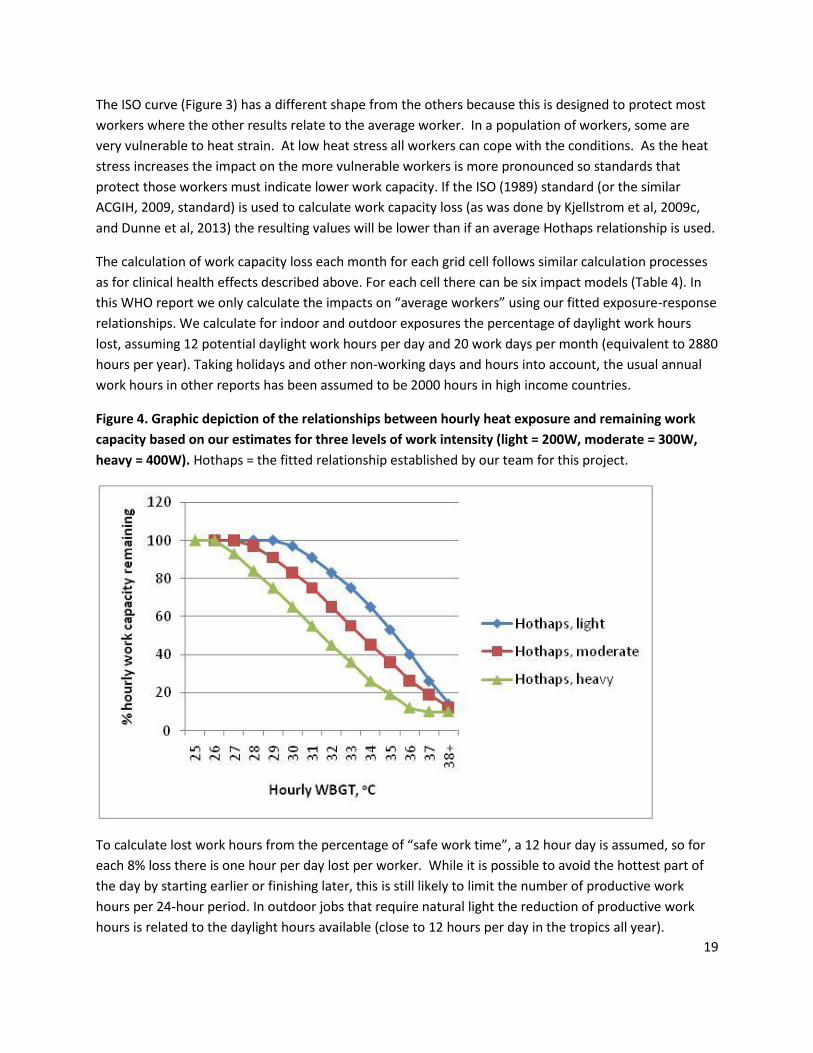
Figure 4. Graphic depiction of the relationships between hourly heat exposure and remaining work

capacity based on our estimates for three levels of work intensity (light = 200W, moderate = 300W,

heavy = 400W). Hothaps = the fitted relationship established by our team for this project.

To calculate lost work hours from the percentage of “safe work time”, a 12 hour day is assumed, so for

each 8% loss there is one hour per day lost per worker. While it is possible to avoid the hottest part of

the day by starting earlier or finishing later, this is still likely to limit the number of productive work

hours per 24-hour period. In outdoor jobs that require natural light the reduction of productive work

hours is related to the daylight hours available (close to 12 hours per day in the tropics all year).

20

Model 4: Regional population estimates and workforce distributions

We estimated population - weighted average exposures (million person-months of specific level heat

exposure) for each of the 21 regions, based on the exposure estimates as described above and the

working age population (age range 15-64 years) in each grid cell for each estimation year (1975, 2030

and 2050; with 2000 for comparison purposes) (Table 5). Age-specific population estimates were

acquired by the WHO team for the age groups 0-4, 5-14, 15-64, 65+ years. The population data at

specific grid cell level was downscaled from larger geographic areas than our grid cells by IIASA (2010)

(data supplied by WHO from IIASA website), which creates uncertainties in the local estimates.

Table 5 shows that the expected increase of working age population, with potential exposure to

occupational heat stress, will be particularly great in parts of Africa, Latin America and Asia. These

increases of the local populations at risk will contribute significantly to the estimated impacts of climate

change.

Table 5. Population (millions; men and women combined) in the 15-64 year working age

range in 1975, 2000, 2030 and 2050 by region (source IIASA = International Institute of

Advanced Systems Analysis: http://www.iiasa.ac.at/Research/ECC/index.html)

Population, millions, age 15-64 Ratio, 2050/1975

Region name 1975 2000 2030 2050

1 Asia, High Income 77 110 98 79 1.0

2 Asia, Central 34 48 74 79 2.3

3 Asia, East 550 896 960 768 1.4

4 Asia, South 426 806 1297 1400 3.3

5 Asia, South East 166 336 491 484 2.9

6 Australasia 9 15 18 20 2.2

7 Caribbean 9 22 27 25 2.8

8 Europe, Central 77 82 77 64 0.83

9 Europe, East 140 150 128 104 0.74

10 Europe, West 217 260 242 218 1.0

11 Lat-America, Andean 13 28 46 49 3.8

12 Lat-America, Central 55 123 197 201 3.7

13 Lat-America, South 23 35 48 49 2.1

14 Lat-America, Tropical 56 117 158 151 2.7

15 North America 137 203 231 241 1.8

16 Africa – North 110 222 437 522 4.7

17 Oceania 2 3 7 8 4.0

18 Africa, Central 19 35 94 139 7.3

19 Africa, East 71 143 340 452 6.4

20 Africa, South 19 38 42 37 1.9

21 Africa, West 73 133 327 419 5.7

World total 2283 3807 5338 5508 2.4

21

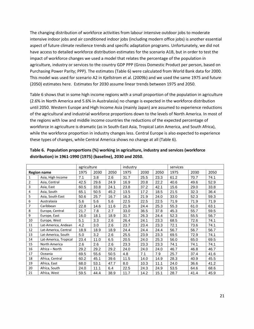
The changing distribution of workforce activities from labour intensive outdoor jobs to moderate

intensive indoor jobs and air conditioned indoor jobs (including modern office jobs) is another essential

aspect of future climate resilience trends and specific adaptation programs. Unfortunately, we did not

have access to detailed workforce distribution estimates for the scenario A1B, but in order to test the

impact of workforce changes we used a model that relates the percentage of the population in

agriculture, industry or services to the country GDP PPP (Gross Domestic Product per person, based on

Purchasing Power Parity; PPP). The estimates (Table 6) were calculated from World Bank data for 2000.

This model was used for scenario A2 in Kjellstrom et al. (2009b) and we used the same 1975 and future

(2050) estimates here. Estimates for 2030 assume linear trends between 1975 and 2050.

Table 6 shows that in some high income regions with a small proportion of the population in agriculture

(2.6% in North America and 5.6% in Australasia) no change is expected in the workforce distribution

until 2050. Western Europe and High Income Asia (mainly Japan) are assumed to experience reductions

of the agricultural and industrial workforce proportions down to the levels of North America. In most of

the regions with low and middle income countries the reductions of the expected percentage of

workforce in agriculture is dramatic (as in South-East Asia, Tropical Latin America, and South Africa),

while the workforce proportion in industry changes less. Central Europe is also expected to experience

these types of changes, while Central America shows no change at all (Table 6).

Table 6. Population proportions (%) working in agriculture, industry and services (workforce

distribution) in 1961-1990 (1975) (baseline), 2030 and 2050.

agriculture industry services

Region name 1975 2030 2050 1975 2030 2050 1975 2030 2050 1 Asia, High Income 7.1 3.8 2.6 31.7 25.5 23.3 61.2 70.7 74.1

2 Asia, Central 42.5 29.6 24.9 16.9 20.8 22.2 40.6 49.6 52.9

3 Asia, East 60.5 33.8 24.1 23.8 37.2 42.1 15.6 29.0 33.8

4 Asia, South 65.1 50.5 45.2 13.5 17.2 18.5 21.5 32.3 36.4

5 Asia, South East 50.6 25.7 16.7 16.3 21.9 24.0 33.0 52.3 59.3

6 Australasia 5.6 5.6 5.6 22.5 22.5 22.5 71.9 71.9 71.9

7 Caribbean 22.8 14.6 11.6 21.9 24.4 25.3 55.3 61.0 63.1

8 Europe, Central 21.7 7.8 2.7 33.0 36.5 37.8 45.3 55.7 59.5

9 Europe, East 16.0 18.1 18.9 31.7 26.3 24.4 52.3 55.5 56.7

10 Europe, West 5.1 3.3 2.6 26.4 24.1 23.3 68.5 72.6 74.1

11 Lat-America, Andean 4.2 3.0 2.6 23.7 23.4 23.3 72.1 73.6 74.1

12 Lat-America, Central 18.9 18.9 18.9 24.4 24.4 24.4 56.7 56.7 56.7

13 Lat-America, South 5.0 3.2 2.6 25.5 23.9 23.3 69.5 72.9 74.1

14 Lat-America, Tropical 23.4 11.0 6.5 20.5 24.0 25.3 56.0 65.0 69.5

15 North America 2.6 2.6 2.6 23.3 23.3 23.3 74.1 74.1 74.1

16 Africa – North 29.2 29.2 29.2 24.0 24.0 24.0 46.7 46.8 46.7

17 Oceania 69.5 55.6 50.5 4.8 7.1 7.9 25.7 37.4 41.6

18 Africa, Central 60.2 45.1 39.6 11.5 14.0 14.9 28.3 40.9 45.5

19 Africa, East 68.0 53.1 47.7 8.0 10.3 11.1 24.0 36.6 41.2

20 Africa, South 24.0 11.1 6.4 22.5 24.3 24.9 53.5 64.6 68.6

21 Africa, West 59.5 44.4 38.9 11.7 14.2 15.1 28.7 41.4 45.9

22

In the calculations of regional heat impacts that include workforce distributions, we have assumed that

agricultural workers are outside in the sun, and that they are required to carry out “heavy labour”

(400W). The corresponding group working in industry are assumed to carry out “moderate labour”

(300W) indoors or in full shade. People in service jobs are assumed to have air conditioning and very

light labour, so their heat exposure is too low to create impacts due to climate change. In fact, many

people in service jobs in low and middle income countries are not protected by air conditioning or other

cooling systems, so our analysis is “conservative” (source: personal observations and information

received by Kjellstrom from key informants in tropical countries). Intellectual tasks in office jobs, or

other service jobs, are also slowed down or negatively affected in other ways (e.g. more errors) by high

workplace heat exposure (Hancock et al., 2007).

The impact of climate change on health and productivity in the whole population is calculated by

“weighted” analysis of impacts in the different workforce groups. If occupational heat stress in 2030

causes an annual mortality risk of 10/million in the “heavy labour” category and 2/million in the

“moderate labour” category, and the respective proportions in the two workforce categories are 50%

and 20%, then the impact in the whole population will be 0.5 x 10 + 0.2 x 2 = 5.4/million. We calculate

these values for 2030 and 2050 for the 21 regions and our result sections show the separate and

combined changes of health risks or work capacity loss due to climate change and workforce change.

Summary of the features of our four models

1. We use grid cell based observed climate data or climate model estimates of temperatures

(monthly average of daily max, daily mean and the half-way point temperatures) and humidity

(average of daily mean dew point) to calculate with model 1 the corresponding monthly WBGT

“in shade” or indoors assuming air movement over skin (wind speed) at 1 m/s and no additional

heat radiation.

2. We use CRU grid cell data (0.5 x 0.5 degrees) for 1975 (based on observed data) to assess the

actual levels of WBGT for each grid cell at that time (1975 is an average of 30 years of monthly

data, 1961-1990).

3. We then use a “field change” method (average change for each region) to add the calculated

change of regional average WBGT to the regional CRU 1975 data to calculate 2030 and 2050 grid

cell WBGT levels in the 21 regions defined by WHO using the three supplied models (averaging

the three runs of the EGMAM model into one estimate, and then using the other two climate

models as independent input: BCM and IPCM).

4. Monthly data for WBGTmax, WBGTmean and WBGThalf (halfway between max and mean), is

used to estimate the person-months and person-hours of heat exposure indoors at each WBGT

one-degree level for a population of 1 million, assuming that each of the three WBGT levels

represent four daylight hours per day during the month.

5. Additional heat exposure outdoors in sunny conditions during the four hottest hours is

estimated by adding 3 oC to the indoor WBGTmax levels.

23

6. For clinical health risk calculations (acute effects) we use the monthly WBGTmax data as

indicators of daily exposures during the afternoons. For the calculation of work capacity loss we

use numbers of hours at different heat exposure levels based on the monthly averages of the

WBGT levels estimates (max, half, mean).

7. For each WBGT level we use exposure-response relationships for fatal and non-fatal health risks

(model 2), to calculate impacts per million working people at three different levels of work

intensity (heavy, moderate and light) for the time points 2030 and 2050. The heat exposure

levels are based on the three climate model outputs for these years (30-year periods around the

years) and the “counter-factual” estimates use the baseline “1975” climate distributions in grid

cells. The difference between calculated risks at 2030 and 2050 climate levels and 1975 climate

levels in the same population is presented as the climate change impacts.

8. We also estimate potential impacts of heat exposure on work capacity and labor productivity

during daylight hours applying different exposure-response relationships to the heat estimates

by region (model 3).

9. Then we can calculate the number of people affected by applying working age population sizes

(ages 15-64 years) and workforce distributions (model 4) for each region (based on grid cells in

the region) at the two time periods (2030 and 2050).

10. The calculated impacts on clinical health and work capacity are discussed and analyzed in

comparison with other analysis results of the consequences of current and future climate

conditions for working people.

Assumptions

Assumptions in the model calculations A number of specific assumptions were applied in the different model calculations and these will not be

repeated here. The project was started in 2009 and most of the analysis of exposures and impacts were

carried out in 2010 and 2011. Therefore the new RCP system of climate modeling was not used (analysis

with these new models is in progress).

The general assumptions included:

The future global economy, demography and society will evolve according to SRES scenario A1B

The data from three climate models (five model runs) provided from WHO were valid examples

of how global climate change will influence regional environmental heat exposures for the

scenario A1B

The heat exposure index used by us (WBGT) is a valid method to express exposures of relevance

to occupational health based on a combination of climate variables

24

The calculation of “in shade” ( indoor) exposures in non-cooled work environments is a valid

way to start estimating average exposure levels for populations of working people

The addition of 3 oC to the in shade values produces reasonable estimates of outdoor exposures

“in sun” for the hottest four hours of the day

The exposure-response relationships established from the few available epidemiological studies

are valid representations of how “average worker” groups would be affected by heat exposures.

Adaptation will take place, but for certain job types protective measures, apart from taking rest

breaks or avoiding work during the hottest periods, will be impossible or too expensive for the

heat exposed working populations. Reduced vulnerability via changes in the workforce

distribution was taken into account with the methods we use.

Because of uncertainties in the input climate data, the exposure-response relationships, and the

actual exposed population sizes, our analysis uses rather basic statistical and mathematical

methods to produce the results. More advanced analysis would not make the results more

accurate.

Adaptation options Ideally if we were to describe and quantify the current and future adaptation to occupational heat

stress, we should have access to regional data or estimates for the time points i.e. 1975, 2030 and 2050

for the following variables. However, valid data of this type is not available at either global or regional

level.

- Distribution of workforce into outdoor and indoor workers, as well as into groups working at

different work intensity

- Availability of air conditioning or other cooling technologies in workplaces

- Local work restrictions related to heat exposure and their enforcement

- Hydration program implementation at each workplace

- Routine use of reliable and non-invasive methods of monitoring heat stress in working people

- Access to medical treatment in case of serious clinical effects of heat

- Other occupational health and safety program activities

Our starting point in this study was to calculate occupational heat stress impacts for three different work

intensity levels (heavy, moderate, light) in “in shade” and “in sun” heat exposure conditions. The results

indicate the impact of climate conditions separate from other workplace changes. As in other health

impact assessments of climate change, we do not have detailed predictions of how other relevant

variables will change (including local adaptation actions or population health status). However, we use

estimates of changes in workforce distributions to assess one important aspect of changing climate

25

resilience that also indicates a potential for adaptation. More use of technology that reduces the need

for heavy labor activities is another important aspect.

For the WHO project we were asked to develop scenarios for heat adaptation that ranged from

“optimistic” (= major adaptation implemented) to “pessimistic” (= no adaptation implemented). In the

case of occupational heat stress impacts, one can assume that adaptation to the increasing heat

exposures will involve increase of rest periods and reduction of average work intensity, which will

potentially prevent most of the clinical heat effects. However, the work capacity loss will then increase

as estimated by our analysis. The exact degree of future application of technology for cooling

workplaces and for reducing work intensity is not known, but it is very unlikely that all occupational heat

stress impacts can be prevented. In addition, it should be pointed out that heat impacts on daily life

activities (collecting water or firewood, gardening, subsistence farming, home industry, etc.) will be of

great importance for billions of people, and air conditioning is not likely to be used in all aspects of daily

life.

It is important to consider the likely adaptation trends in light of other global projections of future

health related infrastructure. The OECD Environmental Outlook report (OECD, 2012) assembled data

and analysis from different UN agencies and other sources and concluded that in 2050 it is likely that

1,400 million people among the 9,000 million inhabitants of the planet at that time will still be without

access to basic sanitation. More than 240 million people will not have access to safe and sufficient

household water (OECD, 2012). These numbers indicate that access to workplace air conditioning or

other cooling systems will also be lacking for hundreds of millions of people. The occupational heat

stress problems due to climate change identified in our analysis will most likely become an additional

burden in the daily life of a vast number of people, and these problems are already affecting life and

well-being of many million people.

Results and comments

Future heat exposure due to climate change

Geographic distribution of occupational heat exposures

Our estimates of occupational heat exposure use grid cell calculations, but the results are generally

presented by region. The great variation in intra-region occupational heat exposures during the hottest

month of 1995 can be seen in Figure 5 (based on CRU real data), where North America, for instance, has

very large differences between the southern states of the USA and the northern states and Canada.

Southern Africa, Australasia and East Asia (mainly China) also have great internal variations in maximum

heat exposure.

26

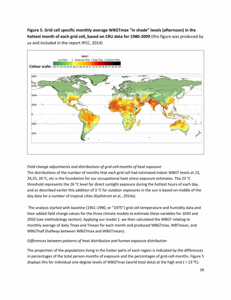
Figure 5. Grid cell specific monthly average WBGTmax “in shade” levels (afternoon) in the

hottest month of each grid cell, based on CRU data for 1980-2009 (this figure was produced by

us and included in the report IPCC, 2014)

Colour scale:

Field change adjustments and distributions of grid-cell-months of heat exposure

The distributions of the number of months that each grid cell had estimated indoor WBGT levels at 23,

24,25, 26 oC, etc is the foundation for our occupational heat stress exposure estimates. The 23 oC

threshold represents the 26 oC level for direct sunlight exposure during the hottest hours of each day,

and as described earlier this addition of 3 oC for outdoor exposures in the sun is based on middle of the

day data for a number of tropical cities (Kjellstrom et al., 2014a).

The analysis started with baseline (1961-1990, or “1975”) grid cell temperature and humidity data and

then added field change values for the three climate models to estimate these variables for 2030 and

2050 (see methodology section). Applying our model 1, we then calculated the WBGT relating to

monthly average of daily Tmax and Tmean for each month and produced WBGTmax, WBTmean, and

WBGThalf (halfway between WBGTmax and WBGTmean).

Differences between patterns of heat distribution and human exposure distribution

The proportion of the populations living in the hotter parts of each region is indicated by the differences

in percentages of the total person-months of exposure and the percentages of grid-cell-months. Figure 5

displays this for individual one-degree levels of WBGTmax (world total data) at the high end ( > 23 oC).

27

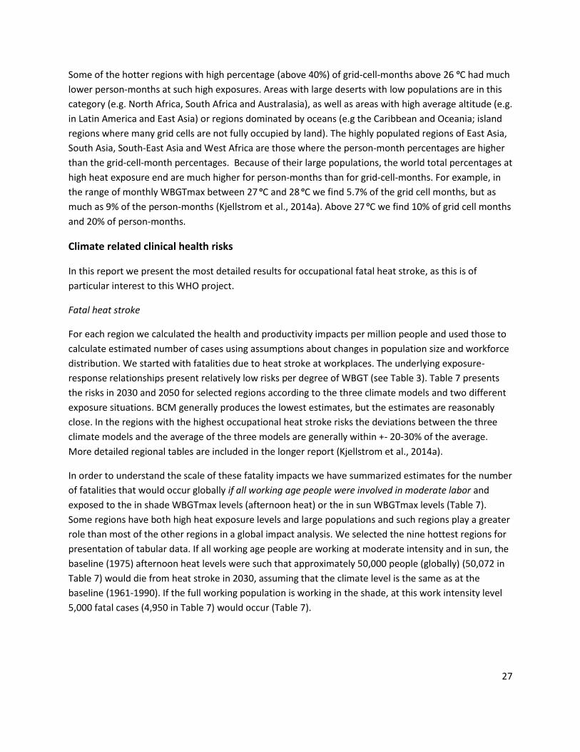
Some of the hotter regions with high percentage (above 40%) of grid-cell-months above 26 oC had much

lower person-months at such high exposures. Areas with large deserts with low populations are in this

category (e.g. North Africa, South Africa and Australasia), as well as areas with high average altitude (e.g.

in Latin America and East Asia) or regions dominated by oceans (e.g the Caribbean and Oceania; island

regions where many grid cells are not fully occupied by land). The highly populated regions of East Asia,

South Asia, South-East Asia and West Africa are those where the person-month percentages are higher

than the grid-cell-month percentages. Because of their large populations, the world total percentages at

high heat exposure end are much higher for person-months than for grid-cell-months. For example, in

the range of monthly WBGTmax between 27 oC and 28 oC we find 5.7% of the grid cell months, but as

much as 9% of the person-months (Kjellstrom et al., 2014a). Above 27 oC we find 10% of grid cell months

and 20% of person-months.

Climate related clinical health risks

In this report we present the most detailed results for occupational fatal heat stroke, as this is of

particular interest to this WHO project.

Fatal heat stroke

For each region we calculated the health and productivity impacts per million people and used those to

calculate estimated number of cases using assumptions about changes in population size and workforce

distribution. We started with fatalities due to heat stroke at workplaces. The underlying exposure-

response relationships present relatively low risks per degree of WBGT (see Table 3). Table 7 presents

the risks in 2030 and 2050 for selected regions according to the three climate models and two different

exposure situations. BCM generally produces the lowest estimates, but the estimates are reasonably

close. In the regions with the highest occupational heat stroke risks the deviations between the three

climate models and the average of the three models are generally within +- 20-30% of the average.

More detailed regional tables are included in the longer report (Kjellstrom et al., 2014a).

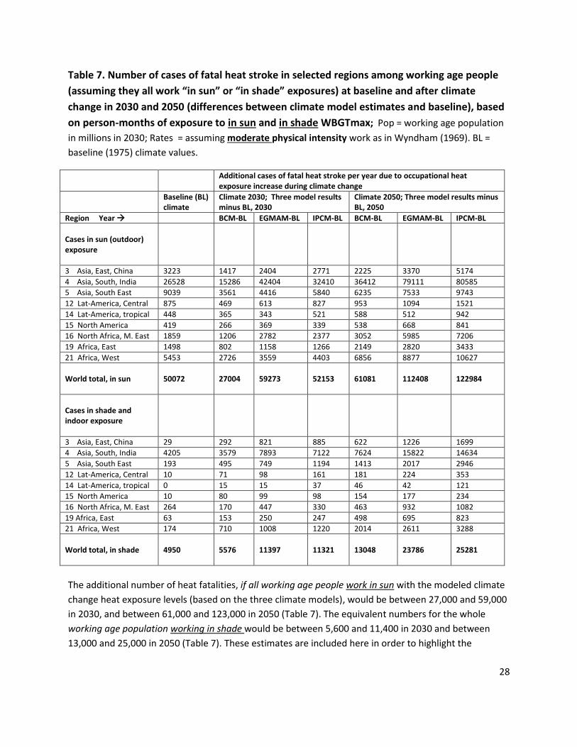
In order to understand the scale of these fatality impacts we have summarized estimates for the number

of fatalities that would occur globally if all working age people were involved in moderate labor and

exposed to the in shade WBGTmax levels (afternoon heat) or the in sun WBGTmax levels (Table 7).

Some regions have both high heat exposure levels and large populations and such regions play a greater

role than most of the other regions in a global impact analysis. We selected the nine hottest regions for

presentation of tabular data. If all working age people are working at moderate intensity and in sun, the

baseline (1975) afternoon heat levels were such that approximately 50,000 people (globally) (50,072 in

Table 7) would die from heat stroke in 2030, assuming that the climate level is the same as at the

baseline (1961-1990). If the full working population is working in the shade, at this work intensity level

5,000 fatal cases (4,950 in Table 7) would occur (Table 7).

28

Table 7. Number of cases of fatal heat stroke in selected regions among working age people

(assuming they all work “in sun” or “in shade” exposures) at baseline and after climate

change in 2030 and 2050 (differences between climate model estimates and baseline), based

on person-months of exposure to in sun and in shade WBGTmax; Pop = working age population

in millions in 2030; Rates = assuming moderate physical intensity work as in Wyndham (1969). BL =

baseline (1975) climate values.

Additional cases of fatal heat stroke per year due to occupational heat exposure increase during climate change

Baseline (BL) climate

Climate 2030; Three model results minus BL, 2030

Climate 2050; Three model results minus BL, 2050

Region Year BCM-BL EGMAM-BL IPCM-BL BCM-BL EGMAM-BL IPCM-BL

Cases in sun (outdoor) exposure 3 Asia, East, China 3223 1417 2404 2771 2225 3370 5174

4 Asia, South, India 26528 15286 42404 32410 36412 79111 80585

5 Asia, South East 9039 3561 4416 5840 6235 7533 9743

12 Lat-America, Central 875 469 613 827 953 1094 1521

14 Lat-America, tropical 448 365 343 521 588 512 942

15 North America 419 266 369 339 538 668 841

16 North Africa, M. East 1859 1206 2782 2377 3052 5985 7206

19 Africa, East 1498 802 1158 1266 2149 2820 3433

21 Africa, West 5453 2726 3559 4403 6856 8877 10627

World total, in sun

50072

27004

59273

52153

61081

112408

122984

Cases in shade and indoor exposure 3 Asia, East, China 29 292 821 885 622 1226 1699

4 Asia, South, India 4205 3579 7893 7122 7624 15822 14634

5 Asia, South East 193 495 749 1194 1413 2017 2946

12 Lat-America, Central 10 71 98 161 181 224 353

14 Lat-America, tropical 0 15 15 37 46 42 121

15 North America 10 80 99 98 154 177 234

16 North Africa, M. East 264 170 447 330 463 932 1082

19 Africa, East 63 153 250 247 498 695 823

21 Africa, West 174 710 1008 1220 2014 2611 3288

World total, in shade

4950

5576

11397

11321

13048

23786

25281

The additional number of heat fatalities, if all working age people work in sun with the modeled climate

change heat exposure levels (based on the three climate models), would be between 27,000 and 59,000

in 2030, and between 61,000 and 123,000 in 2050 (Table 7). The equivalent numbers for the whole

working age population working in shade would be between 5,600 and 11,400 in 2030 and between

13,000 and 25,000 in 2050 (Table 7). These estimates are included here in order to highlight the

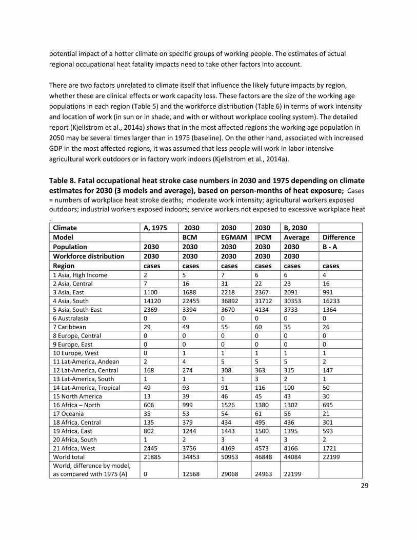
29

potential impact of a hotter climate on specific groups of working people. The estimates of actual

regional occupational heat fatality impacts need to take other factors into account.

There are two factors unrelated to climate itself that influence the likely future impacts by region,

whether these are clinical effects or work capacity loss. These factors are the size of the working age

populations in each region (Table 5) and the workforce distribution (Table 6) in terms of work intensity

and location of work (in sun or in shade, and with or without workplace cooling system). The detailed

report (Kjellstrom et al., 2014a) shows that in the most affected regions the working age population in

2050 may be several times larger than in 1975 (baseline). On the other hand, associated with increased

GDP in the most affected regions, it was assumed that less people will work in labor intensive

agricultural work outdoors or in factory work indoors (Kjellstrom et al., 2014a).

Table 8. Fatal occupational heat stroke case numbers in 2030 and 1975 depending on climate estimates for 2030 (3 models and average), based on person-months of heat exposure; Cases = numbers of workplace heat stroke deaths; moderate work intensity; agricultural workers exposed outdoors; industrial workers exposed indoors; service workers not exposed to excessive workplace heat .

Climate A, 1975 2030 2030 2030 B, 2030

Model BCM EGMAM IPCM Average Difference

Population 2030 2030 2030 2030 2030 B - A

Workforce distribution 2030 2030 2030 2030 2030

Region cases cases cases cases cases cases 1 Asia, High Income 2 5 7 6 6 4

2 Asia, Central 7 16 31 22 23 16

3 Asia, East 1100 1688 2218 2367 2091 991

4 Asia, South 14120 22455 36892 31712 30353 16233

5 Asia, South East 2369 3394 3670 4134 3733 1364

6 Australasia 0 0 0 0 0 0

7 Caribbean 29 49 55 60 55 26

8 Europe, Central 0 0 0 0 0 0

9 Europe, East 0 0 0 0 0 0

10 Europe, West 0 1 1 1 1 1

11 Lat-America, Andean 2 4 5 5 5 2

12 Lat-America, Central 168 274 308 363 315 147

13 Lat-America, South 1 1 1 3 2 1

14 Lat-America, Tropical 49 93 91 116 100 50

15 North America 13 39 46 45 43 30

16 Africa – North 606 999 1526 1380 1302 695

17 Oceania 35 53 54 61 56 21

18 Africa, Central 135 379 434 495 436 301

19 Africa, East 802 1244 1443 1500 1395 593

20 Africa, South 1 2 3 4 3 2

21 Africa, West 2445 3756 4169 4573 4166 1721

World total 21885 34453 50953 46848 44084 22199

World, difference by model, as compared with 1975 (A) 0 12568 29068 24963 22199

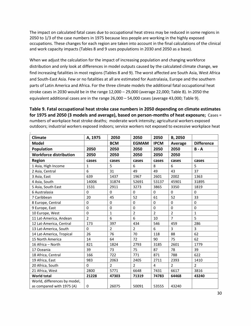
30

The impact on calculated fatal cases due to occupational heat stress may be reduced in some regions in 2050 to 1/3 of the case numbers in 1975 because less people are working in the highly exposed occupations. These changes for each region are taken into account in the final calculations of the clinical and work capacity impacts (Tables 8 and 9 uses populations in 2030 and 2050 as a base). When we adjust the calculation for the impact of increasing population and changing workforce

distribution and only look at differences in model outputs caused by the calculated climate change, we

find increasing fatalities in most regions (Tables 8 and 9). The worst affected are South Asia, West Africa

and South-East Asia. Few or no fatalities at all are estimated for Australasia, Europe and the southern

parts of Latin America and Africa. For the three climate models the additional fatal occupational heat

stroke cases in 2030 would be in the range 12,000 – 29,000 (average 22,000; Table 8). In 2050 the

equivalent additional cases are in the range 26,000 – 54,000 cases (average 43,000; Table 9).

Table 9. Fatal occupational heat stroke case numbers in 2050 depending on climate estimates for 1975 and 2050 (3 models and average), based on person-months of heat exposure; Cases = numbers of workplace heat stroke deaths; moderate work intensity; agricultural workers exposed outdoors; industrial workers exposed indoors; service workers not exposed to excessive workplace heat .

Climate A, 1975 2050 2050 2050 B, 2050

Model BCM EGMAM IPCM Average Difference

Population 2050 2050 2050 2050 2050 B - A

Workforce distribution 2050 2050 2050 2050 2050

Region cases cases cases cases cases cases 1 Asia, High Income 1 5 6 8 6 5

2 Asia, Central 6 31 49 49 43 37

3 Asia, East 639 1437 1967 2601 2002 1363

4 Asia, South 14006 31874 52691 53137 45901 31895

5 Asia, South East 1531 2911 3273 3865 3350 1819

6 Australasia 0 0 0 0 0 0

7 Caribbean 20 45 52 61 52 33

8 Europe, Central 0 0 0 0 0 0

9 Europe, East 0 0 0 0 0 0

10 Europe, West 0 1 2 2 2 1

11 Lat-America, Andean 2 6 6 10 7 5

12 Lat-America, Central 173 397 434 546 459 286

13 Lat-America, South 0 2 2 6 3 3

14 Lat-America, Tropical 26 76 70 118 88 62

15 North America 14 64 72 90 75 62

16 Africa – North 821 1824 2793 3185 2601 1779

17 Oceania 39 73 75 87 78 39

18 Africa, Central 166 722 771 871 788 622

19 Africa, East 983 2063 2405 2711 2393 1410

20 Africa, South 0 2 2 4 2 2

21 Africa, West 2800 5771 6648 7431 6617 3816

World total 21228 47303 71319 74783 64468 43240

World, differences by model, as compared with 1975 (A) 0 26075 50091 53555 43240

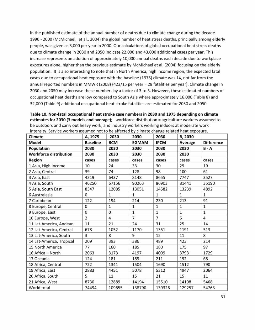
31

In the published estimate of the annual number of deaths due to climate change during the decade

1990 - 2000 (McMichael, et al., 2004) the global number of heat stress deaths, principally among elderly

people, was given as 3,000 per year in 2000. Our calculations of global occupational heat stress deaths

due to climate change in 2030 and 2050 indicate 22,000 and 43,000 additional cases per year. This

increase represents an addition of approximately 10,000 annual deaths each decade due to workplace

exposures alone, higher than the previous estimate by McMichael et al. (2004) focusing on the elderly

population. It is also interesting to note that in North America, high income region, the expected fatal

cases due to occupational heat exposure with the baseline (1975) climate was 14, not far from the

annual reported numbers in MMWR (2008) (423/15 per year = 28 fatalities per year). Climate change in

2030 and 2050 may increase these numbers by a factor of 3 to 5. However, these estimated numbers of

occupational heat deaths are low compared to South Asia where approximately 16,000 (Table 8) and

32,000 (Table 9) additional occupational heat stroke fatalities are estimated for 2030 and 2050.

Table 10. Non-fatal occupational heat stroke case numbers in 2030 and 1975 depending on climate estimates for 2030 (3 models and average); workforce distribution = agriculture workers assumed to be outdoors and carry out heavy work, and industry workers working indoors at moderate work intensity. Service workers assumed not to be affected by climate change related heat exposure.

Climate A, 1975 2030 2030 2030 B, 2030

Model Baseline BCM EGMAM IPCM Average Difference

Population 2030 2030 2030 2030 2030 B - A

Workforce distribution 2030 2030 2030 2030 2030

Region cases cases cases cases cases cases

1 Asia, High Income 10 24 33 30 29 19

2 Asia, Central 39 74 128 98 100 61

3 Asia, East 4219 6437 8148 8655 7747 3527

4 Asia, South 46250 67156 90263 86903 81441 35190

5 Asia, South East 8347 12085 13051 14582 13239 4892

6 Australasia 0 1 1 1 1 1

7 Caribbean 122 194 214 230 213 91

8 Europe, Central 0 1 1 1 1 1

9 Europe, East 0 0 1 1 1 1

10 Europe, West 2 4 7 7 6 4

11 Lat-America, Andean 11 21 24 31 25 14

12 Lat-America, Central 678 1052 1170 1351 1191 513

13 Lat-America, South 3 8 9 15 11 8

14 Lat-America, Tropical 209 393 386 489 423 214

15 North America 77 160 185 180 175 97

16 Africa – North 2063 3173 4197 4009 3793 1729

17 Oceania 124 181 185 211 192 68

18 Africa, Central 722 1341 1504 1690 1512 790

19 Africa, East 2883 4451 5078 5312 4947 2064

20 Africa, South 5 11 15 21 15 11

21 Africa, West 8730 12889 14194 15510 14198 5468

World total 74494 109655 138790 139326 129257 54763

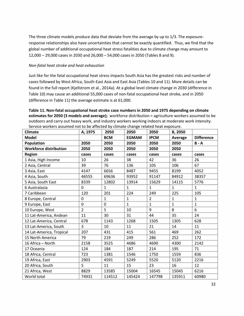
32

The three climate models produce data that deviate from the average by up to 1/3. The exposure-

response relationships also have uncertainties that cannot be exactly quantified. Thus, we find that the

global number of additional occupational heat stress fatalities due to climate change may amount to

12,000 – 29,000 cases in 2030 and 26,000 – 54,000 cases in 2050 (Tables 8 and 9).

Non-fatal heat stroke and heat exhaustion

Just like for the fatal occupational heat stress impacts South Asia has the greatest risks and number of

cases followed by West Africa, South-East Asia and East Asia (Tables 10 and 11). More details can be

found in the full report (Kjellstrom et al., 2014a). At a global level climate change in 2030 (difference in

Table 10) may cause an additional 55,000 cases of non-fatal occupational heat stroke, and in 2050

(difference in Table 11) the average estimate is at 61,000.

Table 11. Non-fatal occupational heat stroke case numbers in 2050 and 1975 depending on climate estimates for 2050 (3 models and average); workforce distribution = agriculture workers assumed to be outdoors and carry out heavy work, and industry workers working indoors at moderate work intensity. Service workers assumed not to be affected by climate change related heat exposure.

Climate A, 1975 2050 2050 2050 B, 2050

Model BCM EGMAM IPCM Average Difference

Population 2050 2050 2050 2050 2050 B - A

Workforce distribution 2050 2050 2050 2050 2050

Region cases cases cases cases cases cases

1 Asia, High Income 10 26 38 42 36 26

2 Asia, Central 39 76 136 105 106 67

3 Asia, East 4147 6656 8487 9455 8199 4052

4 Asia, South 46555 69636 93952 91147 84912 38357

5 Asia, South East 8339 12802 13914 15629 14115 5776

6 Australasia 0 1 1 1 1 1

7 Caribbean 120 201 224 249 225 105

8 Europe, Central 0 1 1 2 1 1

9 Europe, East 0 0 1 1 1 1

10 Europe, West 2 5 10 9 8 6

11 Lat-America, Andean 11 30 31 44 35 24

12 Lat-America, Central 678 1143 1268 1505 1305 628

13 Lat-America, South 3 10 11 21 14 11

14 Lat-America, Tropical 207 431 415 561 469 262

15 North America 79 219 249 286 252 172

16 Africa – North 2158 3525 4686 4690 4300 2142

17 Oceania 124 184 187 214 195 71

18 Africa, Central 723 1381 1546 1750 1559 836

19 Africa, East 2903 4591 5249 5520 5120 2216

20 Africa, South 5 11 15 23 16 12

21 Africa, West 8829 13585 15004 16545 15045 6216

World total 74931 114512 145424 147798 135911 60980

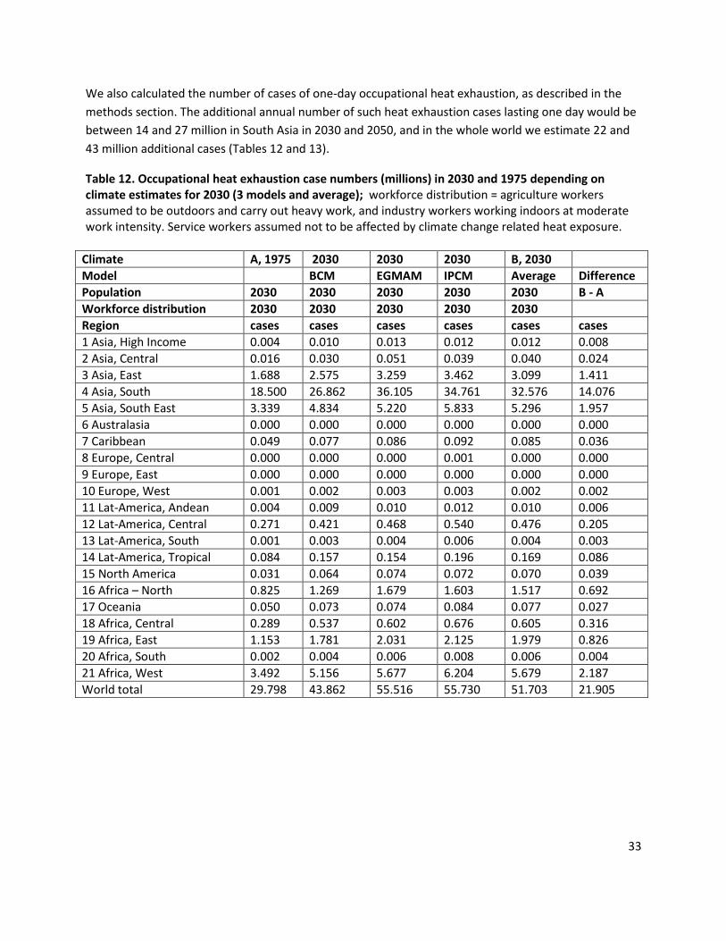
33

We also calculated the number of cases of one-day occupational heat exhaustion, as described in the

methods section. The additional annual number of such heat exhaustion cases lasting one day would be

between 14 and 27 million in South Asia in 2030 and 2050, and in the whole world we estimate 22 and

43 million additional cases (Tables 12 and 13).

Table 12. Occupational heat exhaustion case numbers (millions) in 2030 and 1975 depending on climate estimates for 2030 (3 models and average); workforce distribution = agriculture workers assumed to be outdoors and carry out heavy work, and industry workers working indoors at moderate work intensity. Service workers assumed not to be affected by climate change related heat exposure.

Climate A, 1975 2030 2030 2030 B, 2030

Model BCM EGMAM IPCM Average Difference

Population 2030 2030 2030 2030 2030 B - A

Workforce distribution 2030 2030 2030 2030 2030

Region cases cases cases cases cases cases

1 Asia, High Income 0.004 0.010 0.013 0.012 0.012 0.008

2 Asia, Central 0.016 0.030 0.051 0.039 0.040 0.024

3 Asia, East 1.688 2.575 3.259 3.462 3.099 1.411

4 Asia, South 18.500 26.862 36.105 34.761 32.576 14.076

5 Asia, South East 3.339 4.834 5.220 5.833 5.296 1.957

6 Australasia 0.000 0.000 0.000 0.000 0.000 0.000

7 Caribbean 0.049 0.077 0.086 0.092 0.085 0.036

8 Europe, Central 0.000 0.000 0.000 0.001 0.000 0.000

9 Europe, East 0.000 0.000 0.000 0.000 0.000 0.000

10 Europe, West 0.001 0.002 0.003 0.003 0.002 0.002

11 Lat-America, Andean 0.004 0.009 0.010 0.012 0.010 0.006

12 Lat-America, Central 0.271 0.421 0.468 0.540 0.476 0.205

13 Lat-America, South 0.001 0.003 0.004 0.006 0.004 0.003

14 Lat-America, Tropical 0.084 0.157 0.154 0.196 0.169 0.086

15 North America 0.031 0.064 0.074 0.072 0.070 0.039

16 Africa – North 0.825 1.269 1.679 1.603 1.517 0.692

17 Oceania 0.050 0.073 0.074 0.084 0.077 0.027

18 Africa, Central 0.289 0.537 0.602 0.676 0.605 0.316

19 Africa, East 1.153 1.781 2.031 2.125 1.979 0.826

20 Africa, South 0.002 0.004 0.006 0.008 0.006 0.004

21 Africa, West 3.492 5.156 5.677 6.204 5.679 2.187

World total 29.798 43.862 55.516 55.730 51.703 21.905

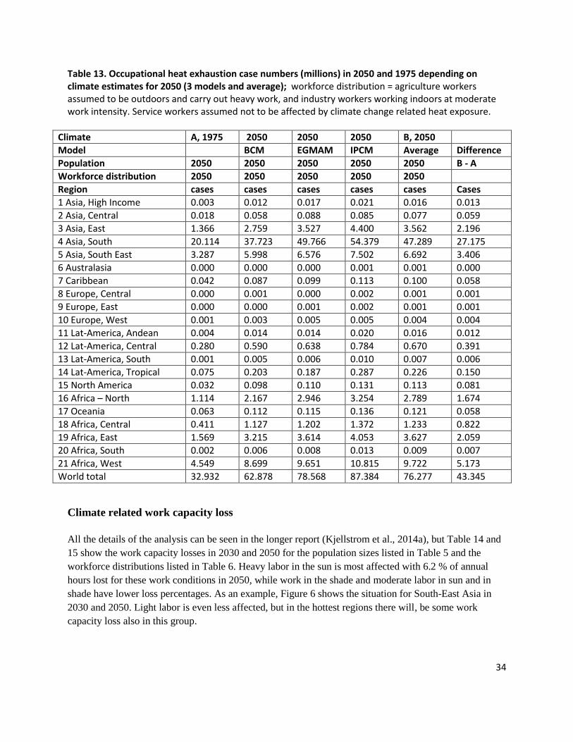
34

Table 13. Occupational heat exhaustion case numbers (millions) in 2050 and 1975 depending on climate estimates for 2050 (3 models and average); workforce distribution = agriculture workers assumed to be outdoors and carry out heavy work, and industry workers working indoors at moderate work intensity. Service workers assumed not to be affected by climate change related heat exposure.

Climate A, 1975 2050 2050 2050 B, 2050

Model BCM EGMAM IPCM Average Difference

Population 2050 2050 2050 2050 2050 B - A

Workforce distribution 2050 2050 2050 2050 2050

Region cases cases cases cases cases Cases

1 Asia, High Income 0.003 0.012 0.017 0.021 0.016 0.013

2 Asia, Central 0.018 0.058 0.088 0.085 0.077 0.059

3 Asia, East 1.366 2.759 3.527 4.400 3.562 2.196

4 Asia, South 20.114 37.723 49.766 54.379 47.289 27.175

5 Asia, South East 3.287 5.998 6.576 7.502 6.692 3.406

6 Australasia 0.000 0.000 0.000 0.001 0.001 0.000

7 Caribbean 0.042 0.087 0.099 0.113 0.100 0.058

8 Europe, Central 0.000 0.001 0.000 0.002 0.001 0.001

9 Europe, East 0.000 0.000 0.001 0.002 0.001 0.001

10 Europe, West 0.001 0.003 0.005 0.005 0.004 0.004

11 Lat-America, Andean 0.004 0.014 0.014 0.020 0.016 0.012

12 Lat-America, Central 0.280 0.590 0.638 0.784 0.670 0.391

13 Lat-America, South 0.001 0.005 0.006 0.010 0.007 0.006

14 Lat-America, Tropical 0.075 0.203 0.187 0.287 0.226 0.150

15 North America 0.032 0.098 0.110 0.131 0.113 0.081

16 Africa – North 1.114 2.167 2.946 3.254 2.789 1.674

17 Oceania 0.063 0.112 0.115 0.136 0.121 0.058

18 Africa, Central 0.411 1.127 1.202 1.372 1.233 0.822

19 Africa, East 1.569 3.215 3.614 4.053 3.627 2.059

20 Africa, South 0.002 0.006 0.008 0.013 0.009 0.007

21 Africa, West 4.549 8.699 9.651 10.815 9.722 5.173

World total 32.932 62.878 78.568 87.384 76.277 43.345

Climate related work capacity loss

All the details of the analysis can be seen in the longer report (Kjellstrom et al., 2014a), but Table 14 and

15 show the work capacity losses in 2030 and 2050 for the population sizes listed in Table 5 and the

workforce distributions listed in Table 6. Heavy labor in the sun is most affected with 6.2 % of annual

hours lost for these work conditions in 2050, while work in the shade and moderate labor in sun and in

shade have lower loss percentages. As an example, Figure 6 shows the situation for South-East Asia in

2030 and 2050. Light labor is even less affected, but in the hottest regions there will, be some work

capacity loss also in this group.

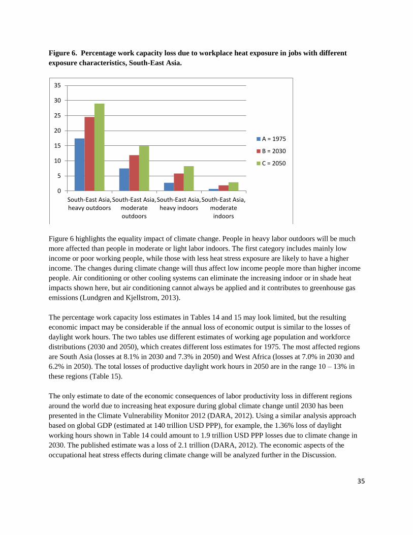
35

Figure 6. Percentage work capacity loss due to workplace heat exposure in jobs with different

exposure characteristics, South-East Asia.

Figure 6 highlights the equality impact of climate change. People in heavy labor outdoors will be much

more affected than people in moderate or light labor indoors. The first category includes mainly low

income or poor working people, while those with less heat stress exposure are likely to have a higher

income. The changes during climate change will thus affect low income people more than higher income

people. Air conditioning or other cooling systems can eliminate the increasing indoor or in shade heat

impacts shown here, but air conditioning cannot always be applied and it contributes to greenhouse gas

emissions (Lundgren and Kjellstrom, 2013).

The percentage work capacity loss estimates in Tables 14 and 15 may look limited, but the resulting

economic impact may be considerable if the annual loss of economic output is similar to the losses of

daylight work hours. The two tables use different estimates of working age population and workforce

distributions (2030 and 2050), which creates different loss estimates for 1975. The most affected regions

are South Asia (losses at 8.1% in 2030 and 7.3% in 2050) and West Africa (losses at 7.0% in 2030 and

6.2% in 2050). The total losses of productive daylight work hours in 2050 are in the range 10 – 13% in

these regions (Table 15).

The only estimate to date of the economic consequences of labor productivity loss in different regions

around the world due to increasing heat exposure during global climate change until 2030 has been

presented in the Climate Vulnerability Monitor 2012 (DARA, 2012). Using a similar analysis approach

based on global GDP (estimated at 140 trillion USD PPP), for example, the 1.36% loss of daylight

working hours shown in Table 14 could amount to 1.9 trillion USD PPP losses due to climate change in

2030. The published estimate was a loss of 2.1 trillion (DARA, 2012). The economic aspects of the

occupational heat stress effects during climate change will be analyzed further in the Discussion.

0

5

10

15

20

25

30

35

South-East Asia,heavy outdoors

South-East Asia,moderateoutdoors

South-East Asia,heavy indoors

South-East Asia,moderate

indoors

A = 1975

B = 2030

C = 2050

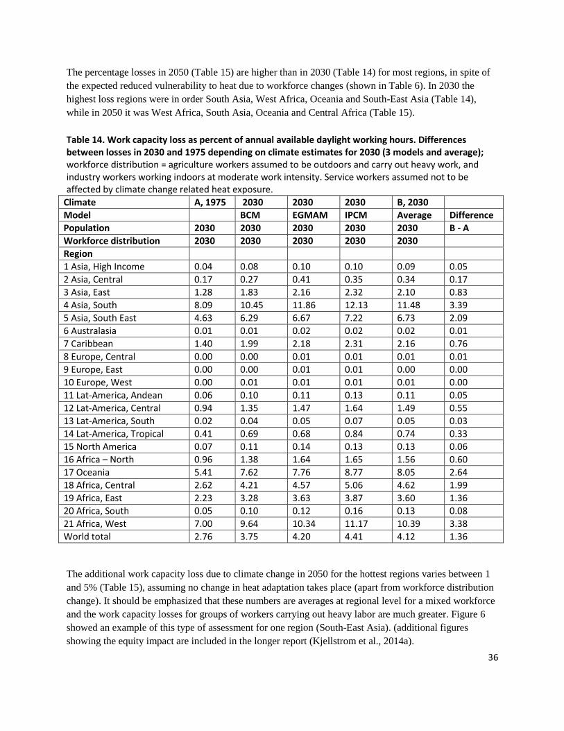
36

The percentage losses in 2050 (Table 15) are higher than in 2030 (Table 14) for most regions, in spite of

the expected reduced vulnerability to heat due to workforce changes (shown in Table 6). In 2030 the

highest loss regions were in order South Asia, West Africa, Oceania and South-East Asia (Table 14),

while in 2050 it was West Africa, South Asia, Oceania and Central Africa (Table 15).

Table 14. Work capacity loss as percent of annual available daylight working hours. Differences between losses in 2030 and 1975 depending on climate estimates for 2030 (3 models and average); workforce distribution = agriculture workers assumed to be outdoors and carry out heavy work, and industry workers working indoors at moderate work intensity. Service workers assumed not to be affected by climate change related heat exposure.

Climate A, 1975 2030 2030 2030 B, 2030

Model BCM EGMAM IPCM Average Difference

Population 2030 2030 2030 2030 2030 B - A

Workforce distribution 2030 2030 2030 2030 2030

Region

1 Asia, High Income 0.04 0.08 0.10 0.10 0.09 0.05

2 Asia, Central 0.17 0.27 0.41 0.35 0.34 0.17

3 Asia, East 1.28 1.83 2.16 2.32 2.10 0.83

4 Asia, South 8.09 10.45 11.86 12.13 11.48 3.39

5 Asia, South East 4.63 6.29 6.67 7.22 6.73 2.09

6 Australasia 0.01 0.01 0.02 0.02 0.02 0.01

7 Caribbean 1.40 1.99 2.18 2.31 2.16 0.76

8 Europe, Central 0.00 0.00 0.01 0.01 0.01 0.01

9 Europe, East 0.00 0.00 0.01 0.01 0.00 0.00

10 Europe, West 0.00 0.01 0.01 0.01 0.01 0.00

11 Lat-America, Andean 0.06 0.10 0.11 0.13 0.11 0.05

12 Lat-America, Central 0.94 1.35 1.47 1.64 1.49 0.55

13 Lat-America, South 0.02 0.04 0.05 0.07 0.05 0.03

14 Lat-America, Tropical 0.41 0.69 0.68 0.84 0.74 0.33

15 North America 0.07 0.11 0.14 0.13 0.13 0.06

16 Africa – North 0.96 1.38 1.64 1.65 1.56 0.60

17 Oceania 5.41 7.62 7.76 8.77 8.05 2.64

18 Africa, Central 2.62 4.21 4.57 5.06 4.62 1.99

19 Africa, East 2.23 3.28 3.63 3.87 3.60 1.36

20 Africa, South 0.05 0.10 0.12 0.16 0.13 0.08

21 Africa, West 7.00 9.64 10.34 11.17 10.39 3.38

World total 2.76 3.75 4.20 4.41 4.12 1.36

The additional work capacity loss due to climate change in 2050 for the hottest regions varies between 1

and 5% (Table 15), assuming no change in heat adaptation takes place (apart from workforce distribution

change). It should be emphasized that these numbers are averages at regional level for a mixed workforce

and the work capacity losses for groups of workers carrying out heavy labor are much greater. Figure 6

showed an example of this type of assessment for one region (South-East Asia). (additional figures

showing the equity impact are included in the longer report (Kjellstrom et al., 2014a).

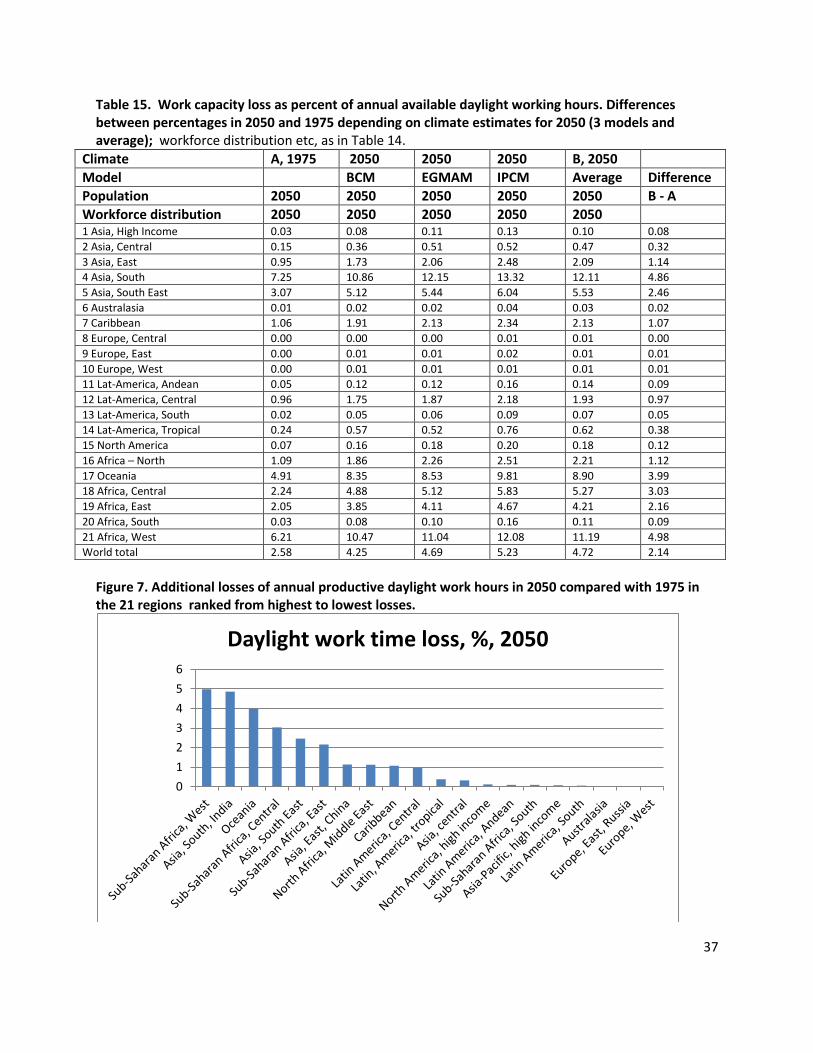
37

Table 15. Work capacity loss as percent of annual available daylight working hours. Differences between percentages in 2050 and 1975 depending on climate estimates for 2050 (3 models and average); workforce distribution etc, as in Table 14.

Climate A, 1975 2050 2050 2050 B, 2050

Model BCM EGMAM IPCM Average Difference

Population 2050 2050 2050 2050 2050 B - A

Workforce distribution 2050 2050 2050 2050 2050 1 Asia, High Income 0.03 0.08 0.11 0.13 0.10 0.08

2 Asia, Central 0.15 0.36 0.51 0.52 0.47 0.32

3 Asia, East 0.95 1.73 2.06 2.48 2.09 1.14

4 Asia, South 7.25 10.86 12.15 13.32 12.11 4.86

5 Asia, South East 3.07 5.12 5.44 6.04 5.53 2.46

6 Australasia 0.01 0.02 0.02 0.04 0.03 0.02

7 Caribbean 1.06 1.91 2.13 2.34 2.13 1.07

8 Europe, Central 0.00 0.00 0.00 0.01 0.01 0.00

9 Europe, East 0.00 0.01 0.01 0.02 0.01 0.01

10 Europe, West 0.00 0.01 0.01 0.01 0.01 0.01

11 Lat-America, Andean 0.05 0.12 0.12 0.16 0.14 0.09

12 Lat-America, Central 0.96 1.75 1.87 2.18 1.93 0.97

13 Lat-America, South 0.02 0.05 0.06 0.09 0.07 0.05

14 Lat-America, Tropical 0.24 0.57 0.52 0.76 0.62 0.38

15 North America 0.07 0.16 0.18 0.20 0.18 0.12

16 Africa – North 1.09 1.86 2.26 2.51 2.21 1.12

17 Oceania 4.91 8.35 8.53 9.81 8.90 3.99

18 Africa, Central 2.24 4.88 5.12 5.83 5.27 3.03

19 Africa, East 2.05 3.85 4.11 4.67 4.21 2.16

20 Africa, South 0.03 0.08 0.10 0.16 0.11 0.09

21 Africa, West 6.21 10.47 11.04 12.08 11.19 4.98

World total 2.58 4.25 4.69 5.23 4.72 2.14

Figure 7. Additional losses of annual productive daylight work hours in 2050 compared with 1975 in the 21 regions ranked from highest to lowest losses.

0

1

2

3

4

5

6

Daylight work time loss, %, 2050

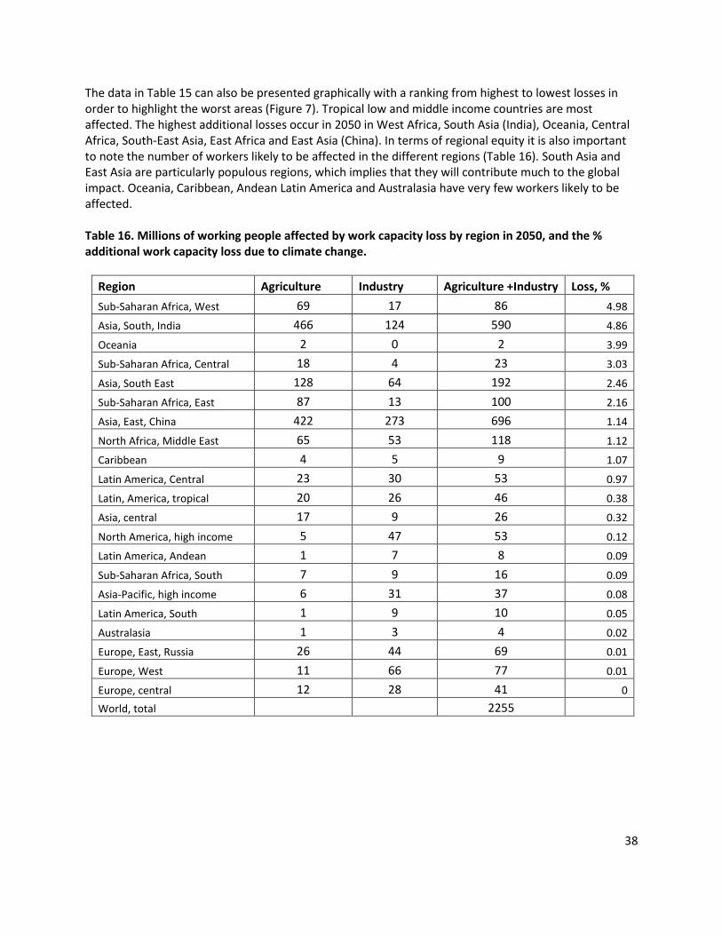
38

The data in Table 15 can also be presented graphically with a ranking from highest to lowest losses in order to highlight the worst areas (Figure 7). Tropical low and middle income countries are most affected. The highest additional losses occur in 2050 in West Africa, South Asia (India), Oceania, Central Africa, South-East Asia, East Africa and East Asia (China). In terms of regional equity it is also important to note the number of workers likely to be affected in the different regions (Table 16). South Asia and East Asia are particularly populous regions, which implies that they will contribute much to the global impact. Oceania, Caribbean, Andean Latin America and Australasia have very few workers likely to be affected. Table 16. Millions of working people affected by work capacity loss by region in 2050, and the % additional work capacity loss due to climate change.

Region Agriculture Industry Agriculture +Industry Loss, %

Sub-Saharan Africa, West 69 17 86 4.98

Asia, South, India 466 124 590 4.86

Oceania 2 0 2 3.99

Sub-Saharan Africa, Central 18 4 23 3.03

Asia, South East 128 64 192 2.46

Sub-Saharan Africa, East 87 13 100 2.16

Asia, East, China 422 273 696 1.14

North Africa, Middle East 65 53 118 1.12

Caribbean 4 5 9 1.07

Latin America, Central 23 30 53 0.97

Latin, America, tropical 20 26 46 0.38

Asia, central 17 9 26 0.32

North America, high income 5 47 53 0.12

Latin America, Andean 1 7 8 0.09

Sub-Saharan Africa, South 7 9 16 0.09

Asia-Pacific, high income 6 31 37 0.08

Latin America, South 1 9 10 0.05

Australasia 1 3 4 0.02

Europe, East, Russia 26 44 69 0.01

Europe, West 11 66 77 0.01

Europe, central 12 28 41 0

World, total 2255

39

Uncertainty

In the WHO guidance for this project four key components of the uncertainty of the results were listed:

Climate model uncertainty

Emission uncertainty

Measurement uncertainty

Process uncertainty

To this we add a fifth which we call Policy uncertainty. It captures the unknown future development of

the world’s population and economy, which will largely determine future workforce composition,

average income (GDP), use of cooling or labor intensity reduction technology, and relevant heat

protection legislation and enforcement (Table 17).

Climate model uncertainly appears to be a relatively minor factor. We have found, as described earlier

that the three climate models we were offered from the WHO team actually showed rather small

differences of proportions at high heat exposure level. In weighted average population based heat

exposure expressed as million person-degrees, the three individual models only differed by

approximately 10% from the 3-model average (Kjellstrom et al., 2014a). The results of impact

calculations with the three models differ more from the average because the impact is not proportional

to exposure. However, the lowest and highest results from the three climate models are always within

±25% of the average.

Emissions uncertainty is a fundamental issue that affects all the health impact assessments. Using just

the A1B scenario in this project may limit the general applicability of our results. Emissions uncertainty

arises from policy uncertainty coupled with future developments in technology, particularly for energy

supply and transport services.

Measurement uncertainty is more related to the specific variables that we have referred to and

calculated. The underlying data for our heat exposure assessments were the annual averages of monthly

climate variables, and as we point out in our analysis the coefficient of variation (SD/mean) for the key

variable, WBGT, was relatively small, a few percent based on a 30-year data set. We conclude that the

underlying measurements were reasonably accurate with a confidence interval 10% around the means.

The process uncertainty emerges from a lack of mechanistic understanding of the cause-effect

relationships that we are quantifying. In the case of heat effects on working people, the physiological

and ergonomic understanding of the mechanisms are well established, but the actual exposure-

response relationships for heat vs. effects are not so well established. The actual uncertainties are

unknown, but one can assume that the uncertainties are no greater than in some of the other

calculations of climate induced health effects (such as malnutrition or vector-borne diseases), which

depend strongly on several assumptions and models.

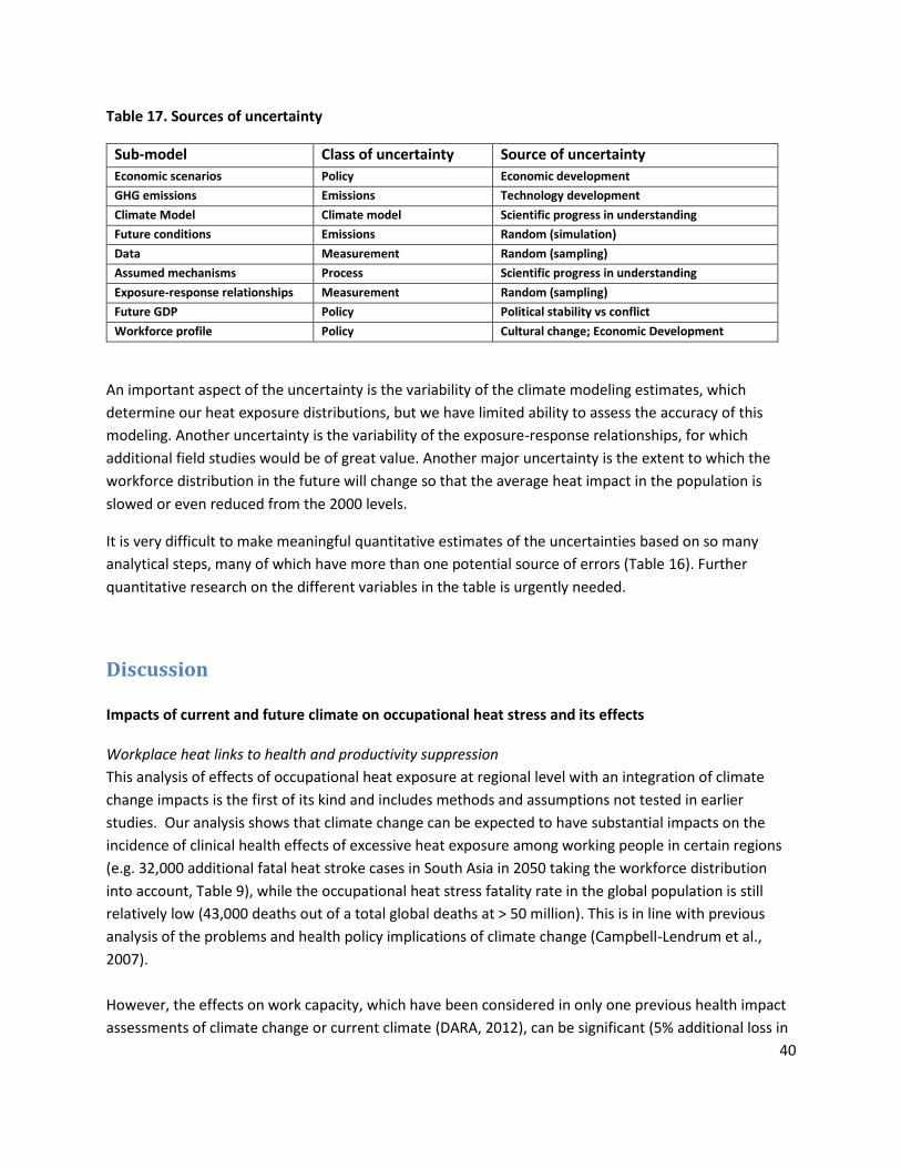
40

Table 17. Sources of uncertainty

Sub-model Class of uncertainty Source of uncertainty

Economic scenarios Policy Economic development

GHG emissions Emissions Technology development

Climate Model Climate model Scientific progress in understanding

Future conditions Emissions Random (simulation)

Data Measurement Random (sampling)

Assumed mechanisms Process Scientific progress in understanding

Exposure-response relationships Measurement Random (sampling)

Future GDP Policy Political stability vs conflict

Workforce profile Policy Cultural change; Economic Development

An important aspect of the uncertainty is the variability of the climate modeling estimates, which

determine our heat exposure distributions, but we have limited ability to assess the accuracy of this

modeling. Another uncertainty is the variability of the exposure-response relationships, for which

additional field studies would be of great value. Another major uncertainty is the extent to which the

workforce distribution in the future will change so that the average heat impact in the population is

slowed or even reduced from the 2000 levels.

It is very difficult to make meaningful quantitative estimates of the uncertainties based on so many

analytical steps, many of which have more than one potential source of errors (Table 16). Further

quantitative research on the different variables in the table is urgently needed.

Discussion Impacts of current and future climate on occupational heat stress and its effects Workplace heat links to health and productivity suppression

This analysis of effects of occupational heat exposure at regional level with an integration of climate

change impacts is the first of its kind and includes methods and assumptions not tested in earlier

studies. Our analysis shows that climate change can be expected to have substantial impacts on the

incidence of clinical health effects of excessive heat exposure among working people in certain regions

(e.g. 32,000 additional fatal heat stroke cases in South Asia in 2050 taking the workforce distribution

into account, Table 9), while the occupational heat stress fatality rate in the global population is still

relatively low (43,000 deaths out of a total global deaths at > 50 million). This is in line with previous

analysis of the problems and health policy implications of climate change (Campbell-Lendrum et al.,

2007).

However, the effects on work capacity, which have been considered in only one previous health impact

assessments of climate change or current climate (DARA, 2012), can be significant (5% additional loss in

41

South Asia and West Africa in 2050, Table 15). Naturally these effects are greatest in people with jobs

that involve heavy labor, while in light labor jobs the changing climate has an impact but with more

limited losses in work capacity. Our analysis of work capacity loss involves effects related to the

physiological function of people carrying out physical activity. It does not yet consider the psychological

exhaustion effects of heat exposure at work, which can be considerable even in light office type work

(see discussions by Wyndham, 1969 and Hancock et al., 2007). The differences in the impacts between

different job types create important challenges to both health and socio-economic equity, exacerbating

the existing health gap between low income outdoor or indoor workers doing hard labor and high

income indoor workers in less physically strenuous jobs.

It is important to consider the potential additional exposures in urban and peri-urban areas where the

urban heat island effect (Oke, 1973) creates higher heat exposure levels than those estimated via the

grid cell modeling used by WHO in this project. The WBGT levels in urban areas may be 3 oC higher than

the grid cell estimates, but extensive heat exposure monitoring programs are needed to get more

accurate exposure estimates. In addition to extra heat exposure the urban and peri-urban workers may

also face urban air pollution (especially photochemical oxidants), which creates clinical health risks and

possibly work capacity loss. There is evidence that the two exposures create additive effects (e.g. Dear

et al., 2005). There is also research in progress analyzing the increasing air pollution levels in urban areas

as a result of increasing heat levels.

The mean estimates of the global number of additional occupational heat stroke fatalities is 22,000 in

2030 (Table 8, range 12,000 – 29,000) and 43,000 in 2050 (Table 9, range 26,000 – 54,000). These

numbers show a doubling of the annual occupational heat stroke fatalities in 2030 and a further

doubling in 2050. Compared with the calculations of the potential mortality impact of climate change

from 1990 to 2000 (3,000 deaths in mainly elderly age groups; McMichael et al., 2004) these numbers

are large, but no previous estimates of the occupational mortality are available. Emerging data from the

USA (MMWR, 2008), India (Nag et al., 2009) and Qatar (Gibson and Pattison, 2014) indicate that further

mortality analysis is of importance for making more accurate estimates. Appropriate preventive policies

and actions can reduce the occupational heat stroke problems already now, but the prevention of

clinical health effects may reduce labor productivity unless efficient methods to reduce work intensity or

to cool workplaces are applied.

An important health impact for the affected communities will be the likely work capacity and labor

productivity loss. The current loss of 6 – 7 % of workable daylight hours each year (or an additional loss

due to climate change of 5 %) (Table 15) in regions like South Asia and West Africa will cause major

problems for the local community to keep economic activities going all year around. For individual low

income families any income loss caused by climate conditions will reduce the resources available for

safe drinking water, sanitation, nutrition, and other health protecting daily needs and the family health

will suffer.

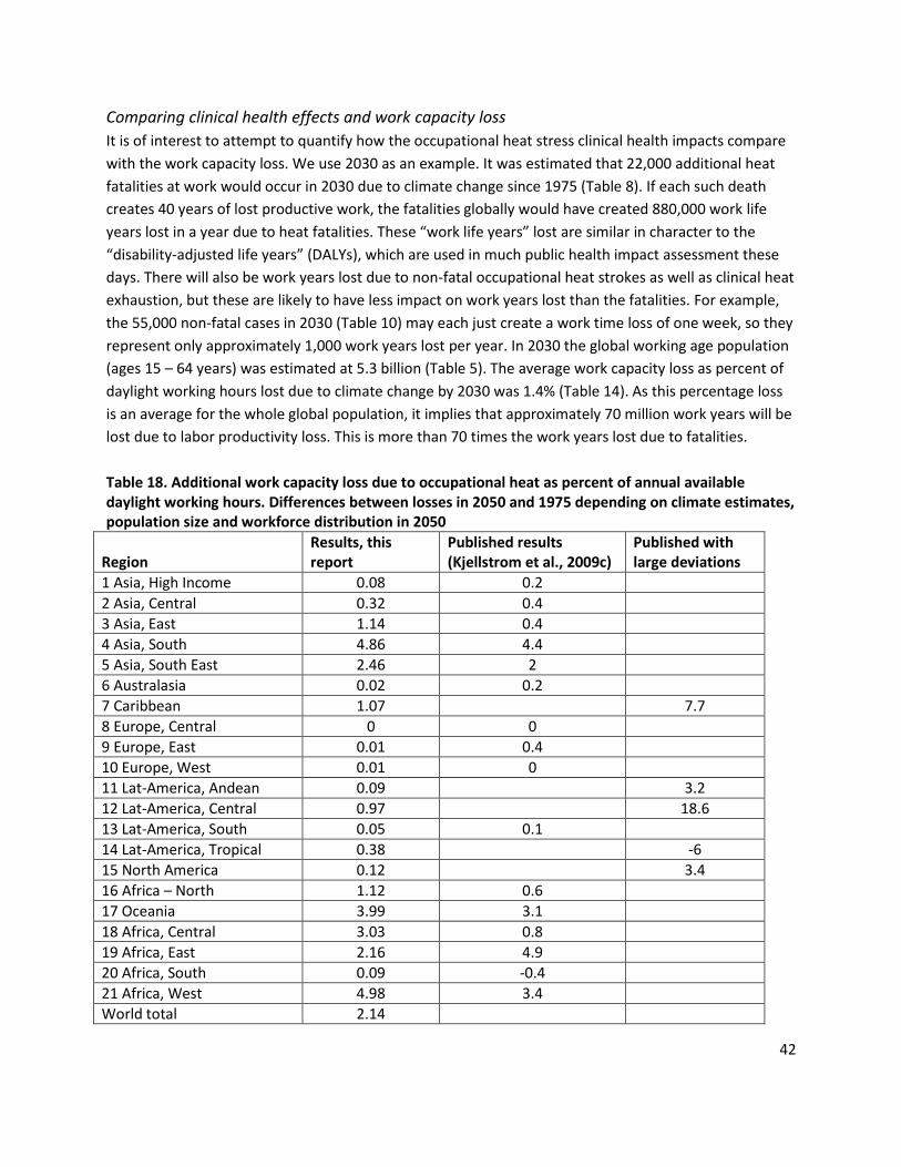
42

Comparing clinical health effects and work capacity loss

It is of interest to attempt to quantify how the occupational heat stress clinical health impacts compare

with the work capacity loss. We use 2030 as an example. It was estimated that 22,000 additional heat

fatalities at work would occur in 2030 due to climate change since 1975 (Table 8). If each such death

creates 40 years of lost productive work, the fatalities globally would have created 880,000 work life

years lost in a year due to heat fatalities. These “work life years” lost are similar in character to the

“disability-adjusted life years” (DALYs), which are used in much public health impact assessment these

days. There will also be work years lost due to non-fatal occupational heat strokes as well as clinical heat

exhaustion, but these are likely to have less impact on work years lost than the fatalities. For example,

the 55,000 non-fatal cases in 2030 (Table 10) may each just create a work time loss of one week, so they

represent only approximately 1,000 work years lost per year. In 2030 the global working age population

(ages 15 – 64 years) was estimated at 5.3 billion (Table 5). The average work capacity loss as percent of

daylight working hours lost due to climate change by 2030 was 1.4% (Table 14). As this percentage loss

is an average for the whole global population, it implies that approximately 70 million work years will be

lost due to labor productivity loss. This is more than 70 times the work years lost due to fatalities.

Table 18. Additional work capacity loss due to occupational heat as percent of annual available daylight working hours. Differences between losses in 2050 and 1975 depending on climate estimates, population size and workforce distribution in 2050

Region Results, this report

Published results (Kjellstrom et al., 2009c)

Published with large deviations

1 Asia, High Income 0.08 0.2

2 Asia, Central 0.32 0.4

3 Asia, East 1.14 0.4

4 Asia, South 4.86 4.4

5 Asia, South East 2.46 2

6 Australasia 0.02 0.2

7 Caribbean 1.07 7.7

8 Europe, Central 0 0

9 Europe, East 0.01 0.4

10 Europe, West 0.01 0

11 Lat-America, Andean 0.09 3.2

12 Lat-America, Central 0.97 18.6

13 Lat-America, South 0.05 0.1

14 Lat-America, Tropical 0.38 -6

15 North America 0.12 3.4

16 Africa – North 1.12 0.6

17 Oceania 3.99 3.1

18 Africa, Central 3.03 0.8

19 Africa, East 2.16 4.9

20 Africa, South 0.09 -0.4

21 Africa, West 4.98 3.4

World total 2.14

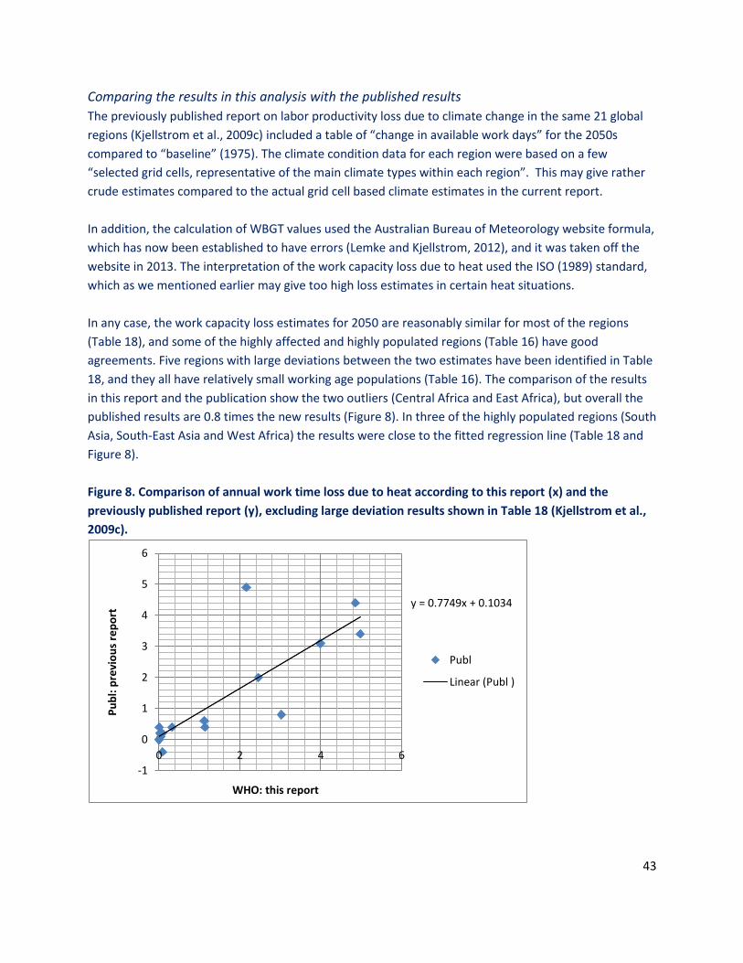
43

Comparing the results in this analysis with the published results

The previously published report on labor productivity loss due to climate change in the same 21 global

regions (Kjellstrom et al., 2009c) included a table of “change in available work days” for the 2050s

compared to “baseline” (1975). The climate condition data for each region were based on a few

“selected grid cells, representative of the main climate types within each region”. This may give rather

crude estimates compared to the actual grid cell based climate estimates in the current report.

In addition, the calculation of WBGT values used the Australian Bureau of Meteorology website formula,

which has now been established to have errors (Lemke and Kjellstrom, 2012), and it was taken off the

website in 2013. The interpretation of the work capacity loss due to heat used the ISO (1989) standard,

which as we mentioned earlier may give too high loss estimates in certain heat situations.

In any case, the work capacity loss estimates for 2050 are reasonably similar for most of the regions

(Table 18), and some of the highly affected and highly populated regions (Table 16) have good

agreements. Five regions with large deviations between the two estimates have been identified in Table

18, and they all have relatively small working age populations (Table 16). The comparison of the results

in this report and the publication show the two outliers (Central Africa and East Africa), but overall the

published results are 0.8 times the new results (Figure 8). In three of the highly populated regions (South

Asia, South-East Asia and West Africa) the results were close to the fitted regression line (Table 18 and

Figure 8).

Figure 8. Comparison of annual work time loss due to heat according to this report (x) and the

previously published report (y), excluding large deviation results shown in Table 18 (Kjellstrom et al.,

2009c).

y = 0.7749x + 0.1034

-1

0

1

2

3

4

5

6

0 2 4 6

Pu

bl:

pre

vio

us

rep

ort

WHO: this report

Publ

Linear (Publ )

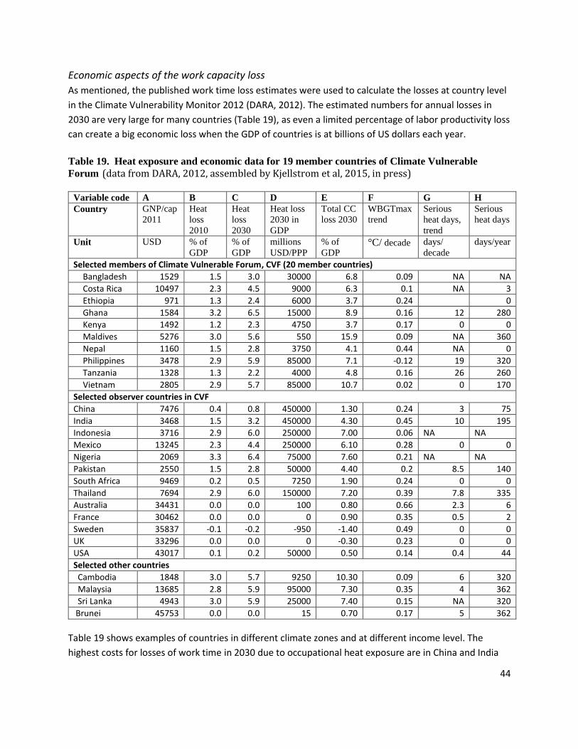
44

Economic aspects of the work capacity loss

As mentioned, the published work time loss estimates were used to calculate the losses at country level

in the Climate Vulnerability Monitor 2012 (DARA, 2012). The estimated numbers for annual losses in

2030 are very large for many countries (Table 19), as even a limited percentage of labor productivity loss

can create a big economic loss when the GDP of countries is at billions of US dollars each year.

Table 19. Heat exposure and economic data for 19 member countries of Climate Vulnerable

Forum (data from DARA, 2012, assembled by Kjellstrom et al, 2015, in press)

Variable code A B C D E F G H

Country GNP/cap

2011

Heat

loss

2010

Heat

loss

2030

Heat loss

2030 in

GDP

Total CC

loss 2030

WBGTmax

trend

Serious

heat days,

trend

Serious

heat days

Unit USD % of

GDP

% of

GDP

millions

USD/PPP

% of

GDP °C/ decade days/

decade

days/year

Selected members of Climate Vulnerable Forum, CVF (20 member countries)

Bangladesh 1529 1.5 3.0 30000 6.8 0.09 NA NA

Costa Rica 10497 2.3 4.5 9000 6.3 0.1 NA 3

Ethiopia 971 1.3 2.4 6000 3.7 0.24 0

Ghana 1584 3.2 6.5 15000 8.9 0.16 12 280

Kenya 1492 1.2 2.3 4750 3.7 0.17 0 0

Maldives 5276 3.0 5.6 550 15.9 0.09 NA 360

Nepal 1160 1.5 2.8 3750 4.1 0.44 NA 0

Philippines 3478 2.9 5.9 85000 7.1 -0.12 19 320

Tanzania 1328 1.3 2.2 4000 4.8 0.16 26 260

Vietnam 2805 2.9 5.7 85000 10.7 0.02 0 170

Selected observer countries in CVF

China 7476 0.4 0.8 450000 1.30 0.24 3 75

India 3468 1.5 3.2 450000 4.30 0.45 10 195

Indonesia 3716 2.9 6.0 250000 7.00 0.06 NA NA

Mexico 13245 2.3 4.4 250000 6.10 0.28 0 0

Nigeria 2069 3.3 6.4 75000 7.60 0.21 NA NA

Pakistan 2550 1.5 2.8 50000 4.40 0.2 8.5 140

South Africa 9469 0.2 0.5 7250 1.90 0.24 0 0

Thailand 7694 2.9 6.0 150000 7.20 0.39 7.8 335

Australia 34431 0.0 0.0 100 0.80 0.66 2.3 6

France 30462 0.0 0.0 0 0.90 0.35 0.5 2

Sweden 35837 -0.1 -0.2 -950 -1.40 0.49 0 0

UK 33296 0.0 0.0 0 -0.30 0.23 0 0

USA 43017 0.1 0.2 50000 0.50 0.14 0.4 44

Selected other countries

Cambodia 1848 3.0 5.7 9250 10.30 0.09 6 320

Malaysia 13685 2.8 5.9 95000 7.30 0.35 4 362

Sri Lanka 4943 3.0 5.9 25000 7.40 0.15 NA 320

Brunei 45753 0.0 0.0 15 0.70 0.17 5 362

Table 19 shows examples of countries in different climate zones and at different income level. The

highest costs for losses of work time in 2030 due to occupational heat exposure are in China and India

45

(450 billion USD PPP per year), but several other countries have estimated multi-billion USD losses (e.g.

Bangladesh, the Philippines, Vietnam, Indonesia, Mexico, Nigeria, Pakistan, Thailand, USA, Malaysia and

Sri Lanka).

These data are tentative, because of the way they were created from the published work time loss

estimates by Kjellstrom et al (2009c), but it is the only available detailed analysis of national economic

impact of climate change effects on working people. Decision-making and policy development for this

aspect of climate change will be significantly assisted by an updated more precise analysis for each

country. Funding for such analysis has been applied for without any meaningful response so far.

In terms of the cost benefit of financial support for improved analysis, one can consider the example of

Malaysia, where the estimated cost of labor productivity loss due to increased workplace heat with

climate change is 95 billion USD in 2030. Let’s assume that this number is in fact 10 times higher than

the real cost, because 90% of the impact is eliminated with climate adaptation. There is still 9.5 billion in

cost for lost productivity. If new analysis and research on this topic can reduce the cost by 10%, then the

value of such work would be 950 million USD per year in 2030. The cost of such work now could be less

than 1 million USD for one country analysis, or even multi-country analysis.

So, is this an attractive cost-benefit relationship to consider in Malaysia (or any other country):

1 million USD analysis work now savings of 950 million USD per year in 2030, or even bigger savings

For the USA, the savings from 1 million dollars in analysis and research investment could be 500 million

USD per year, using this calculation basis, and in China and India the savings could be several billion USD.

The economic aspects of the occupational heat stress impacts of climate change are still poorly

developed, even though recently for the first time an analysis was published for the USA (Kopp et al.,

2014). Adaptation to climate change and mitigation efforts will, of course, require considerable

economic investments, but the reduction of the costs of losses of labor productivity may balance off all

or a large part of such costs.

Policies and practices to reduce climate change impacts

Our results section showed that heat stress will increase due to global heating with substantial increases

of clinical health risks and with major reductions of worker productivity during hot seasons. Adaptation

to these negative impacts will vary from region to region. It is expected that there will be almost

complete adaptation to occupational heat stress in high income countries in temperate climate regions,

while there will be minimal adaptation possible in many jobs in tropical regions.

Temperate zone adaptation

Physical acclimatization to increasing heat should be possible in temperate regions, possibly to the

extent currently existing in hot tropical countries, but the physiological limits will remain in the future.

46

Adaptation to hot summer hours may include starting work earlier, taking breaks during the hot part of

the day and resuming work in the late afternoon or early evening. This is already common practice in

“siesta” countries, but hourly productivity during work hours in the middle of the day will be reduced.

Full air conditioning indoors will relieve heat stress but adds to the outside heat in urban areas as heat is

pumped from buildings into streets (Grimmond, 2007). Air conditioning adds to the energy use (and

contributes to global warming) except where new renewable energy methods are employed: for

example, “free cooling” using phase change (Raj and Velraj, 2010), the use of reflective coatings

especially on roofs (Shen et al., 2011), and systems using solar radiation as energy source (Chan et al.,

2010). A reduction of the urban heat island effect could counteract global warming on a local scale.

Increased tree planting and other vegetation cover is very effective (Grimm et al., 2008) and very

noticeable in some cities (such as Buenos Aries) where there are some tree lined streets and others with

no trees. Water features also contribute to local cooling via water evaporation, but this may increase

local humidity levels that increase WBGT and other heat stress indexes.

Adaptation will be most effective at the local level (CCD, 2009). Effective heat exposure warnings need

to be developed that work for a local community. A new heat stress index like UTCI (Universal Thermal

Climate Index; see: www.utci.org) is likely to require time before it becomes widely used, and familiar

local heat indexes like WBGT, Humidex and the Heat Index will still be used. While heat stress indexes

in different regions do not need to be the same, some quality control is needed so that the heat stress

index is applicable anywhere in the world and valid at local level. In addition, recalculation formulas that

can convert one index number to another need to be freely available. Some published calculation

formulas for WBGT have been incorrect, and different formulas need to be compared and assessed

(Lemke and Kjellstrom, 2012).

Education is needed because many people still believe that sweating cools you down rather than

understanding that evaporation of the sweat is necessary for cooling. Humans are not able to sense

high humidity as accurately as we sense high temperature (Parsons, 2014) and if a large amount of un-

evaporated sweat is mistaken as effective cooling, exposed individuals will fail to take necessary

precautions against heat.

Social adaptation is also important to protect the vulnerable from heat stress (Yardley et al., 2011).

Studies of heat impacts on elderly people in temperate climates identify two risk groups: those who live

isolated lives and those who have low socioeconomic status. We have identified another risk group:

people working in heavy physical intensity jobs without cooling systems, a group that often has low

socio-economic status.

In the USA it is suggested that public interventions generally have less effect on low socio-economic

groups (Ebi and Semenza, 2008). While some adaptations (e.g. heat stress regulations) need a top-down

approach, such as government regulations with proper enforcement, many adaptations “will be more

effective if designed, implemented and monitored with strong community engagement.” (Ebi and

Semenza, 2008). Occupational heat stress protection guidelines are available in a number of countries

47

(e.g. for USA it is ACGIH, 2009), but their implementation needs to involve the exposed worker groups.

Local monitoring of heat stress indexes is becoming increasingly feasible with access to low cost

temperature and humidity dataloggers (see: www.ClimateCIP.org).

Adaptation in the tropics

As the duration of daylight in tropical areas does not vary much from 12 hours there is less opportunity

to compensate for heat impacts during the middle of the day by starting work early or finishing late,

unless major lighting equipment is easily available. A siesta/rest break during the hottest part of the day

truly results in lost opportunities for work that requires daylight. Evaporative cooling is less effective

with the high humidity common in tropical areas (and cooling systems do not reduce the humidity).

However, buildings can be designed differently with roof ventilation (Susanti et al., 2011) and by the

construction of traditional style buildings rather than modern buildings. As the life-time of a new

building is about 50 years, changes to the architecture of buildings need to be implemented now to cope

with the expected temperature rise by 2050.

Nag et al (2009) did extensive research on the vulnerability of Western India to heat stress from climate

change and the potential for adaptation. Their report showed that fatalities due to heat stroke among

farmers were about 11% of the total rural casualties at the workplace. Most heat related mortality

occurred outdoors mainly among those who live in rural areas at the poverty threshold. This is in

contrast to the heat waves in Europe where most fatalities were in urban areas. Nag et al (2009) state

that “there is a lack of health surveillance” in most states of India, and that “the public recognition of the

magnitude of the hazards of [heat strain] remains at a minimum level.” Furthermore, “most people

come to believe that the natural phenomena are unavoidable, and therefore, the heat related mortality

that might be grave during a particular year in a region does not leave a lasting reminder …”. The most

vulnerable people are “urban and rural poor who cannot afford shelters … and those living alone who

cannot access cooling systems” (Nag et al., 2009). Data from several worker groups (Iron workers,

Ceramic workers and Stone Quarry workers) showed that “different forms of artificial hot atmospheres

often exceeded the climatic stresses found even in these extreme natural climates.”

Workplace climate conditions in places without effective air-conditioning, are a combination of the local

heat source contributions and the outdoor “natural” climates. If outdoor heat exposure increases by 1 oC, the combined heat exposure indoors will also increase by 1 oC causing additional heat stress. It is

difficult to quantify the degree of adaptation possible where work processes produce substantial heat

exposure. Clearly adaptation via education and properly enforced regulations on occupational heat

stress can make a significant difference in reducing death and injury from heat stress, such adaptations

are likely to reduce worker productivity and add to the burden of poverty.

In this initial analysis we have assumed that the changes in the workforce distribution will correspond to

the “adaptation” that involves reducing the heavy labour input into the economic activities and

protecting those in service jobs by cooling systems. It is not possible at this time to foresee if any other

adaptation to climate change, that would reduce occupational heat stress and its effects, will take place

in the vulnerable regions.

48

Recent projections of the likely future continued lack of access to safe drinking water and basic

sanitation (OECD, 2012) indicates that many hundreds of millions of people are likely to also suffer from

lack of protection against occupational heat stress. Unless the vulnerability to health impacts from

climate conditions is substantially reduced via significant investments in community infrastructure for

low income people anywhere in the world, the climate change impacts will remain a major challenge for

these people. There will always be a limit to the extent that adaptation can reduce health and

productivity risks, and climate change mitigation is therefore an urgent issue to address.

Conclusions

Occupational heat stress is an important component of impacts of climate conditions on human health.

Working people create internal surplus heat in the body, which adds to the heat stress caused by the

ambient climate. Therefore, working people are a vulnerable group as climate change brings an increase

of very hot days. The physiological and ergonomical evidence about heat effects on human bodies is

very substantial, and the direct effects of heat in a defined working population can be estimated with

more confidence than some of the indirect effects on health from climate change.

Four different types of health effects from climate conditions and climate change are estimated in this

report: heat stroke fatalities, non-fatal serious heat effects, short-term heat exhaustion, and work

capacity loss due to excessive heat exposure, which leads to income loss and greater vulnerability to

adverse health conditions. Using grid cell based climate and population data for 30-year periods around

1975, 2030 and 2050, the quantitative effects on the working age population in 21 geographical regions

and the global total were calculated.

The estimated numbers of additional occupational heat stress fatalities due to climate change are

22,000 in 2030 and 43,000 in 2050 (averages), implying a doubling and quadrupling of cases compared

to 1975. There may be three times as many non-fatal heat stress cases, as well as more than 40 million

daily heat exhaustion cases. If each fatality implies a loss of 40 work life years for the person who died

from occupational heat stroke, the global loss of work years due to climate change in 2030 would be

880,000 work life years. Non-fatal clinical heat effects add just a small number of lost work life years.

The global loss of work capacity (or labor productivity) during daylight working hours could be 1.4 % in

2030 and 2.1 % in 2050. This may look small, but, if GDP is reduced at a similar rate and with an

estimated global GDP in 2030 of 140 trillion USD, 1.4 % loss means a loss of 2 trillion USD of economic

output. The global loss of work life years in 2030 among the 5 billion working age people would be 70

million years (1.4% x 5 billion). This is more than 70 times greater than the work life years lost due to

clinical heat effects.

For most of the 21 global regions the new estimates of labor productivity loss (as % of daylight work

hours) are similar to an earlier published report. Economic cost estimates for different countries based

on the previously published report need to be updated. The global economic cost estimates are similar,

which gives some confidence in the overall analysis method. The losses of health and economic

49

resources can be reduced by climate change adaptation and mitigation. Further analysis work and

adaptation and mitigation advice is urgently needed.

References ACGIH (2009). TLVs for chemical substances and physical agents & Biological exposure indicators. Cincinatti, American Conference of Government Industrial Hygienists.

Bennet C, McMichael T (2010). Non-heat related impacts of climate change on working populations. Global Health Action, Dec 17;3. doi: 10.3402/gha.v3i0.5640. Bernard TE, Pourmoghani M (1999) Prediction of Workplace Wet Bulb Global Temperature. Applied Occupational and Environmental Hygiene 14: 126-134 Berry HL, Bowen K, Kjellstrom T (2010). Climate change and mental health: a causal pathways framework. Int J Public Health, 55: 123-132, (DOI: 10.1007/s00038-009-0112-0) Brice T, Hall T (2009) Wet-bulb calculator. http://www.srh.noaa.gov/epz/?n=wxcalc Bridger RS (2003). Introduction to ergonomics, 2nd edition. London: Taylor & Francis; 2003. Campbell-Lendrum D, Corvalan C, Neira M (2007) Global climate change: implications for international public health policy. Bull World Health Org, 85, 235-237. Chan HY, Riffat SB, Zhu J (2010). Review of passive solar heating and cooling technologies. Renewable and Sustainable Energy Reviews 14: 781-789 Costello A, Abbas M, Allen A, Ball S, Bell S, Bellamy R, et al. (2009) (Lancet-University College London Institute for Global Health Commission). Managing the health effects of climate change. The Lancet 373: 1693-1733. Dear K, Ranmuthugala G, Kjellstrom T, Skinner C and Hanigan I. (2005) Effects of temperature and ozone on daily mortality during the August 2003 heat wave in France. Arch. Environ Occup Health, 60: 205-212. Dell M, Jones BF, Olken BA (2009). Temperature and income: reconciling new cross-sectional and panel estimates. Amer. Econ Rev 99: 198-204. DoLNZ (1997) Guidelines for the management of work in extremes of temperature. 1997. Occupational Safety and health, Department of Labour, Wellington, New Zealand. P.91.ISBN 0-477-03605-8 Dunne JP, Stoufer RJ, John JG. (2013) Reductions in labour capacity from heat stress under climate warming. Nature Climate Change 2013, DOI 10.1038/NCLIMATE1827. Ebi KI, Semenza JC (2008). Community-based adaptation to the health impacts of climate change. Am J Preventative Medicine 35: 501 – 507 Fiala D, Havenith G, Broede P, Kampmann B, Jendritzky G (2011). UTCI-Fiala mulit-node model of human heat transfer and temerpature regulation. Int J Biometeorology. (on website). Fussel H-M, Klein RJT, Ebi KL (2006) Adaptation assessment for public health. In: Menne B. and Ebi KL, Eds. Climate change and adaptation strategies for human health. Darmstadt, Steinkopff Verlag, pp. 41-62.

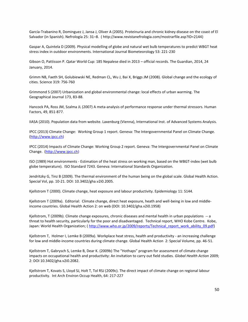
50

García-Trabanino R, Dominguez J, Jansa J, Oliver A (2005). Proteinuria and chronic kidney disease on the coast of El Salvador (in Spanish). Nefrología 25: 31–8. ( http://www.revistanefrologia.com/mostrarfile.asp?ID=2144) Gaspar A, Quintela D (2009). Physical modelling of globe and natural wet bulb temperatures to predict WBGT heat stress index in outdoor environments. International Journal Biometeorology 53: 221-230 Gibson O, Pattisson P. Qatar World Cup: 185 Nepalese died in 2013 – official records. The Guardian, 2014, 24

January, 2014.

Grimm NB, Faeth SH, Golubiewski NE, Redman CL, Wu J, Bai X, Briggs JM (2008). Global change and the ecology of cities. Science 319: 756-760 Grimmond S (2007) Urbanization and global environmental change: local effects of urban warming. The Geographical Journal 173, 83-88. Hancock PA, Ross JM, Szalma JL (2007) A meta-analysis of performance response under thermal stressors. Human Factors, 49, 851-877. IIASA (2010). Population data from website. Laxenburg (Vienna), International Inst. of Advanced Systems Analysis. IPCC (2013) Climate Change: Working Group 1 report. Geneva: The Intergovernmental Panel on Climate Change. (http://www.ipcc.ch) IPCC (2014) Impacts of Climate Change: Working Group 2 report. Geneva: The Intergovernmental Panel on Climate Change. (http://www.ipcc.ch) ISO (1989) Hot environments - Estimation of the heat stress on working man, based on the WBGT-index (wet bulb globe temperature). ISO Standard 7243. Geneva: International Standards Organization. Jendritzky G, Tinz B (2009). The thermal environment of the human being on the global scale. Global Health Action. Special Vol, pp. 10-21. DOI: 10.3402/gha.v2i0.2005. Kjellstrom T (2000). Climate change, heat exposure and labour productivity. Epidemiology 11: S144. Kjellstrom T (2009a). Editorial: Climate change, direct heat exposure, heath and well-being in low and middle-income countries. Global Health Action 2: on web (DOI: 10.3402/gha.v2i0.1958) Kjellstrom, T (2009b). Climate change exposures, chronic diseases and mental health in urban populations -- a threat to health security, particularly for the poor and disadvantaged. Technical report, WHO Kobe Centre. Kobe, Japan: World Health Organization; ( http://www.who.or.jp/2009/reports/Technical_report_work_ability_09.pdf) Kjellstrom T, Holmer I, Lemke B (2009a). Workplace heat stress, health and productivity - an increasing challenge for low and middle-income countries during climate change. Global Health Action 2: Special Volume, pp. 46-51. Kjellstrom T, Gabrysch S, Lemke B, Dear K. (2009b) The “Hothaps” program for assessment of climate change impacts on occupational health and productivity: An invitation to carry out field studies. Global Health Action 2009; 2: DOI 10.3402/gha.v2i0.2082. Kjellstrom T, Kovats S, Lloyd SJ, Holt T, Tol RSJ (2009c). The direct impact of climate change on regional labour productivity. Int Arch Environ Occup Health, 64: 217-227

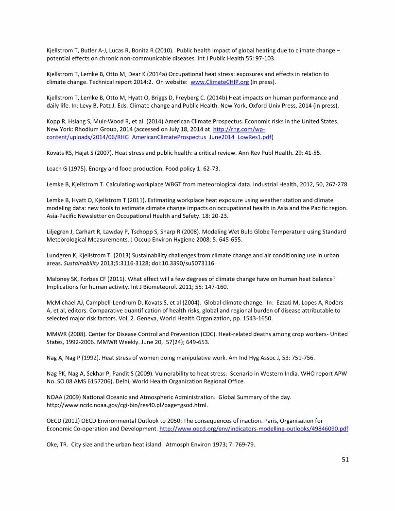
51

Kjellstrom T, Butler A-J, Lucas R, Bonita R (2010). Public health impact of global heating due to climate change – potential effects on chronic non-communicable diseases. Int J Public Health 55: 97-103. Kjellstrom T, Lemke B, Otto M, Dear K (2014a) Occupational heat stress: exposures and effects in relation to climate change. Technical report 2014:2. On website: www.ClimateCHIP.org (in press). Kjellstrom T, Lemke B, Otto M, Hyatt O, Briggs D, Freyberg C. (2014b) Heat impacts on human performance and daily life. In: Levy B, Patz J. Eds. Climate change and Public Health. New York, Oxford Univ Press, 2014 (in press). Kopp R, Hsiang S, Muir-Wood R, et al. (2014) American Climate Prospectus. Economic risks in the United States. New York: Rhodium Group, 2014 (accessed on July 18, 2014 at http://rhg.com/wp-content/uploads/2014/06/RHG_AmericanClimateProspectus_June2014_LowRes1.pdf) Kovats RS, Hajat S (2007). Heat stress and public health: a critical review. Ann Rev Publ Health. 29: 41-55. Leach G (1975). Energy and food production. Food policy 1: 62-73. Lemke B, Kjellstrom T. Calculating workplace WBGT from meteorological data. Industrial Health, 2012, 50, 267-278. Lemke B, Hyatt O, Kjellstrom T (2011). Estimating workplace heat exposure using weather station and climate modeling data: new tools to estimate climate change impacts on occupational health in Asia and the Pacific region. Asia-Pacific Newsletter on Occupational Health and Safety. 18: 20-23. Liljegren J, Carhart R, Lawday P, Tschopp S, Sharp R (2008). Modeling Wet Bulb Globe Temperature using Standard Meteorological Measurements. J Occup Environ Hygiene 2008; 5: 645-655. Lundgren K, Kjellstrom T. (2013) Sustainability challenges from climate change and air conditioning use in urban areas. Sustainability 2013;5:3116-3128; doi:10.3390/su5073116 Maloney SK, Forbes CF (2011). What effect will a few degrees of climate change have on human heat balance? Implications for human activity. Int J Biometeorol. 2011; 55: 147-160. McMichael AJ, Campbell-Lendrum D, Kovats S, et al (2004). Global climate change. In: Ezzati M, Lopes A, Roders A, et al, editors. Comparative quantification of health risks, global and regional burden of disease attributable to selected major risk factors. Vol. 2. Geneva, World Health Organization, pp. 1543-1650. MMWR (2008). Center for Disease Control and Prevention (CDC). Heat-related deaths among crop workers- United States, 1992-2006. MMWR Weekly. June 20, 57(24); 649-653. Nag A, Nag P (1992). Heat stress of women doing manipulative work. Am Ind Hyg Assoc J, 53: 751-756. Nag PK, Nag A, Sekhar P, Pandit S (2009). Vulnerability to heat stress: Scenario in Western India. WHO report APW No. SO 08 AMS 6157206). Delhi, World Health Organization Regional Office. NOAA (2009) National Oceanic and Atmospheric Administration. Global Summary of the day. http://www.ncdc.noaa.gov/cgi-bin/res40.pl?page=gsod.html. OECD (2012) OECD Environmental Outlook to 2050: The consequences of inaction. Paris, Organisation for Economic Co-operation and Development. http://www.oecd.org/env/indicators-modelling-outlooks/49846090.pdf Oke, TR. City size and the urban heat island. Atmosph Environ 1973; 7: 769-79.

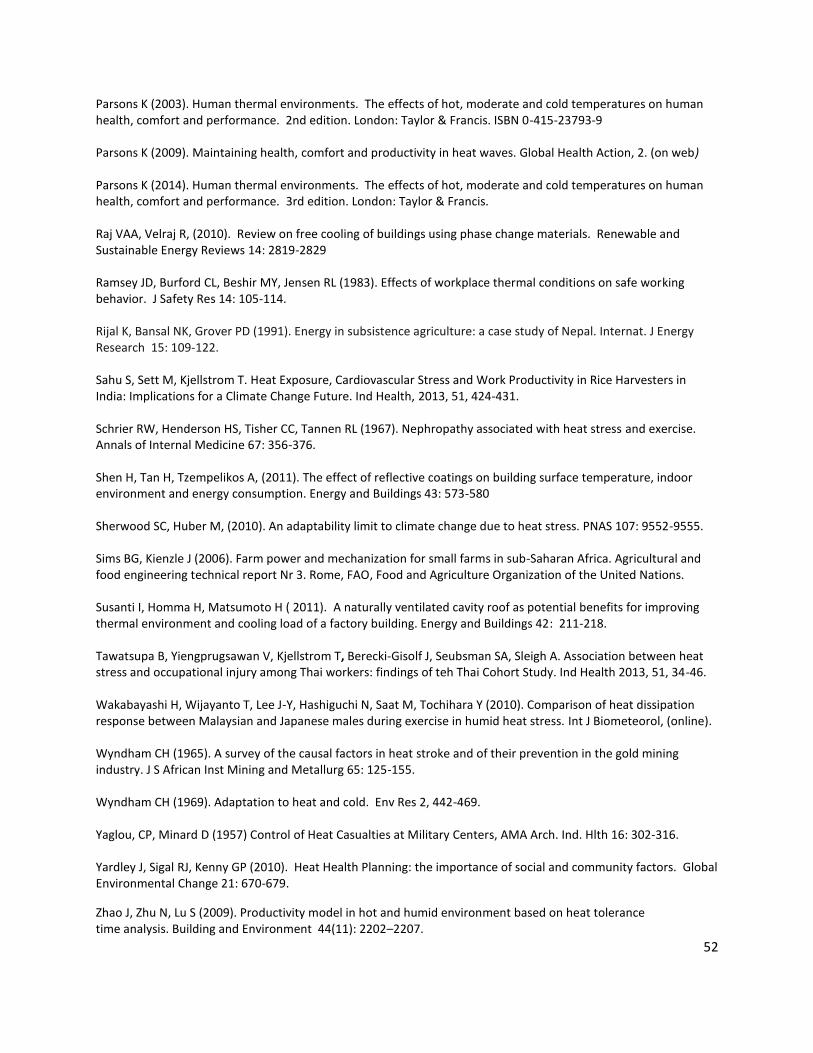
52

Parsons K (2003). Human thermal environments. The effects of hot, moderate and cold temperatures on human health, comfort and performance. 2nd edition. London: Taylor & Francis. ISBN 0-415-23793-9

Parsons K (2009). Maintaining health, comfort and productivity in heat waves. Global Health Action, 2. (on web)

Parsons K (2014). Human thermal environments. The effects of hot, moderate and cold temperatures on human health, comfort and performance. 3rd edition. London: Taylor & Francis.

Raj VAA, Velraj R, (2010). Review on free cooling of buildings using phase change materials. Renewable and Sustainable Energy Reviews 14: 2819-2829 Ramsey JD, Burford CL, Beshir MY, Jensen RL (1983). Effects of workplace thermal conditions on safe working behavior. J Safety Res 14: 105-114. Rijal K, Bansal NK, Grover PD (1991). Energy in subsistence agriculture: a case study of Nepal. Internat. J Energy Research 15: 109-122. Sahu S, Sett M, Kjellstrom T. Heat Exposure, Cardiovascular Stress and Work Productivity in Rice Harvesters in India: Implications for a Climate Change Future. Ind Health, 2013, 51, 424-431. Schrier RW, Henderson HS, Tisher CC, Tannen RL (1967). Nephropathy associated with heat stress and exercise. Annals of Internal Medicine 67: 356-376. Shen H, Tan H, Tzempelikos A, (2011). The effect of reflective coatings on building surface temperature, indoor environment and energy consumption. Energy and Buildings 43: 573-580 Sherwood SC, Huber M, (2010). An adaptability limit to climate change due to heat stress. PNAS 107: 9552-9555. Sims BG, Kienzle J (2006). Farm power and mechanization for small farms in sub-Saharan Africa. Agricultural and food engineering technical report Nr 3. Rome, FAO, Food and Agriculture Organization of the United Nations. Susanti I, Homma H, Matsumoto H ( 2011). A naturally ventilated cavity roof as potential benefits for improving thermal environment and cooling load of a factory building. Energy and Buildings 42: 211-218. Tawatsupa B, Yiengprugsawan V, Kjellstrom T, Berecki-Gisolf J, Seubsman SA, Sleigh A. Association between heat stress and occupational injury among Thai workers: findings of teh Thai Cohort Study. Ind Health 2013, 51, 34-46. Wakabayashi H, Wijayanto T, Lee J-Y, Hashiguchi N, Saat M, Tochihara Y (2010). Comparison of heat dissipation response between Malaysian and Japanese males during exercise in humid heat stress. Int J Biometeorol, (online). Wyndham CH (1965). A survey of the causal factors in heat stroke and of their prevention in the gold mining industry. J S African Inst Mining and Metallurg 65: 125-155. Wyndham CH (1969). Adaptation to heat and cold. Env Res 2, 442-469. Yaglou, CP, Minard D (1957) Control of Heat Casualties at Military Centers, AMA Arch. Ind. Hlth 16: 302-316. Yardley J, Sigal RJ, Kenny GP (2010). Heat Health Planning: the importance of social and community factors. Global Environmental Change 21: 670-679.

Zhao J, Zhu N, Lu S (2009). Productivity model in hot and humid environment based on heat tolerance time analysis. Building and Environment 44(11): 2202–2207.