Technical Report 08-12 Oil drift and fate modelling off NE and NW

www.dmi.dk/dmi/tr08-12 page 1 of 41

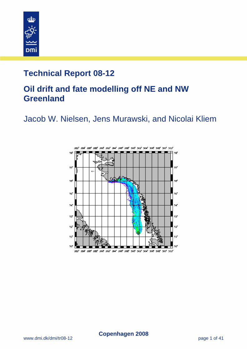
Technical Report 08-12

Oil drift and fate modelling off NE and NW Greenland Jacob W. Nielsen, Jens Murawski, and Nicolai Kliem

Copenhagen 2008



Colophon Serial title: Technical Report 08-12 Title: Oil drift and fate modelling off NE and NW Greenland Subtitle: Author(s): Jacob W. Nielsen, Jens Murawski, and Nicolai Kliem Other contributors: Responsible institution: Danish Meteorological Institute Language: English Keywords: Oil drift, Modelling, Greenland Url: www.dmi.dk/dmi/tr08-12 ISSN: 1399-1388 (online) Version: 3.0 Website: www.dmi.dk Copyright:



Content: Abstract ................................................................................................................................................4 Resumé.................................................................................................................................................4 1. Introduction......................................................................................................................................5 2. DMI oil drift and fate model ............................................................................................................6

Oil particles ......................................................................................................................................6 Oil composition................................................................................................................................7 Drift..................................................................................................................................................7 The oil slick......................................................................................................................................7 Weathering.......................................................................................................................................7 Settling and emigration ....................................................................................................................8 Drift model output............................................................................................................................8 Gridding ...........................................................................................................................................8 Slick thickness and oil concentration...............................................................................................8 Oil in ice-covered waters .................................................................................................................9 Validity ............................................................................................................................................9

3. Model set-up ..................................................................................................................................10 4. Simulations ....................................................................................................................................11 5. Wind periods ..................................................................................................................................12 6. Sea ice conditions ..........................................................................................................................13

Baffin Bay ......................................................................................................................................13 Greenland Sea ................................................................................................................................14

7. Results............................................................................................................................................15 Oil leaving the model domain........................................................................................................15 Surface versus bottom release........................................................................................................15 Oil in ice.........................................................................................................................................15 Drift................................................................................................................................................16 Spreading .......................................................................................................................................16 Downward mixing .........................................................................................................................16 Oil thickness...................................................................................................................................17 Oil composition..............................................................................................................................17 Settling ...........................................................................................................................................17 Oil concentration............................................................................................................................17 Theoretical and practical experience..............................................................................................18 Instantaneous spill..........................................................................................................................18

8. Conclusion .....................................................................................................................................19 Appendix A. Wind conditions ...........................................................................................................20 Appendix B. Case study.....................................................................................................................23 Appendix C. Maximum surface layer oil thickness...........................................................................29 Appendix D. Instantaneous spill ........................................................................................................36 Appendix E. Maximum surface layer oil thickness for instantaneous spill.......................................39 References..........................................................................................................................................41 Previous reports..................................................................................................................................41



Abstract One-month simulations of hypothetical oil spills in two areas east and west of Greenland results in estimates of the region affected, and the maximum skin layer thickness and oil concentration to occur under different wind conditions. Resumé Månedslange simuleringer af hypotetiske oliespild i to grønlandske shelfområder resulterer i en vurdering af hvilket område der påvirkes, den maksimale tykkelse af oliefilm på overfladen, og de højeste koncentrationer af olie, der opnås



1. Introduction This report deals with oil drift simulations in two regions at Greenland, focusing on the shelf regions in the Baffin Bay and the Greenland Sea. The calculations are done with an oil drift model, which simulates the physical and chemical processes a hypothetical oil spill undergoes during the first days after the oil has been released into sea water, and subsequently calculates the drift of the oil for an extended period. Prerequisites for the oil drift model are detailed knowledge of the surface wind and the 3-dimensional motion of the sea, as obtained from the operational numerical weather prediction model HIRLAM, and the operational ocean model HYCOM, respectively. Oil spill conditions and a number of spill sites have been prescribed by the Danish National Envi-ronmental Research Institute, in order to represent envisaged oil spill conditions. Three study periods within the design year medio 2004 – medio 2005, with a wide range of wind conditions, have been selected by the Danish Meteorological Institute. A similar study has been performed previously, see [1] and [2] for descriptions of the oil drift simulations and the operational met-ocean model set-up, respectively. In this study, we use the same basic model set-up as in [1] and [2], with the modification that sea ice is accounted for in the met-ocean forcing of the oil drift model. This modifies the ocean currents that transport and dis-perse the oil. In comparison with [1] two new areas of interest have been selected. The work has been funded by the Danish National Environmental Research Institute (NERI) as part of the cooperation between NERI and the Bureau of Minerals and Petroleum, Greenland Home Rule, on developing a Strategic Environmental Impact Assessment of oil activities.



2. DMI oil drift and fate model Since the 1990’ies, DMI has run an operational oil drift forecasting service for the North Sea – Baltic Sea. In recent years this service has been extended by application of an oil drift and fate model (below referred to as DMOD), that in addition to passive advection simulates a number of chemical processes, collectively termed ‘oil weathering’. The model applies surface winds and 3-dimensional ocean motion (horizontal and vertical current), in order to calculate the drift of the oil. DMOD has been developed specifically for this region, which in winter and spring includes ice-covered waters, by the Bundesamt für Seeschiffahrt und Hydrographie (BSH) in Germany [3]. Recently, DMOD has been generalised and set up for the Greenland waters. The forcing fields are obtained from the DMI large-scale numerical weather prediction model Hirlam-T, which covers all of the arctic and sub-arctic region, and the general 3-dimensional hydrodynamical ocean model HYCOM (HYbrid Coordinate Ocean Model), developed by the University of Miami and the Los Alamos National Laboratory. DMOD runs decoupled from the weather and ocean models. With an extensive archive of HYCOM output data files, any period may be selected for spill studies once the drift model sub-region is properly defined. The processes handled by DMOD are passive drift of oil, horizontal spreading, horizontal and vertical dispersion (by turbulent and buoyant motion), evaporation, emulsification (uptake of sea water), and settling on the bottom or at the shore. Dissolution and oxidation (by sunlight) are considered less important and are not included. Biodegradation is assumed to be important on long timescales only and is also not modelled. The oil will either settle or stay in the water phase, and the only way oil can disappear from the simulations is by evaporation or emigration out of the model domain. A special procedure for taking influence of sea ice on the oil drift into account has been implemented for this study (see below). The oil is released into sea water at a fixed location (latitude, longitude, depth) either instantane-ously or at a fixed rate during a specified time interval. The ambient water temperature influences both weathering and spreading processes. The environment is represented by water of constant temperature and density. A brief summary of processes modelled by DMOD is given below. A detailed description of the processes and parameterizations are given in [3].

Oil particles An oil spill is represented by a large number of particles, each of which has mass, volume and composition that change due to evaporation and emulsification processes. The total release may be envisaged as a particle ‘cloud’. Each oil particle represents a small fraction of the total release; this can be quite a large amount of oil, depending on the magnitude of the release. A particle can not be subdivided but is treated as an entity, unable to interact with other particles. It is assumed to have a disc-like shape, with an area and thickness that increase and decrease respectively, as the oil spreads out horizontally. The particle thickness at the time of its release is 3 cm.



Oil composition An oil particle is composed of 7 groups of hydrocarbon compounds and a residuum. The initial composition constitutes an oil type. DMOD has 8 pre-defined oil types: 4 different crude oils and 4 fuel oils. The density of the oil is the weighted mean of the density of each compound. The compo-sition and the physical properties of the oil, changes with time due to weathering processes (see below).

Drift The oil particles drift passively with the ocean current. In a shallow surface layer the horizontal current is modified by adding a wind-induced logarithmic velocity profile, which at the surface takes its maximum value of 3% of the wind speed. This compensates for the fact that due to finite vertical resolution, the flow in the top layer may not be well resolved vertically by the ocean model itself. This wind-drift is reduced by in the presence of sea ice depending of the ice concentration. Both current and wind velocity are subject to turbulent motion, modelled as random processes scaled by the velocity itself. Turbulence and sub-grid scale motion are further modelled by random walk, by giving the particles a small motion on top of the passive drift, so that all particles do not experience exactly the same drift vector. This spreads out the particle cloud with time, even in total absence of wind or sea current.

The oil slick Each oil particle gradually spreads out due to gravity/viscous forces and surface tension. The slick spreads out in three phases: initially the radius r increases by buoyancy-inertia forces, then, as the slick grows thinner, the spreading moves into a buoyancy-viscous regime, and the final stage is governed by viscosity and surface tension. The oil slick thickness decides which spreading phase is active. The slick area depends on the (strictly theoretically based) slick radius as A=πr². The limit-ing area (and thus thickness) of the slick depends on total spill volume as A [m²] = 105V¾ [m³]. Under constant wind and current, an instantaneous spill takes an asymmetric disk-like shape, elongated in the drift direction, while a continuous spill will resemble smoke from a chimney.

Weathering An oil particle undergoes weathering processes that begin to act immediately or shortly after its release. Weathering processes is the collective term for oil spreading, evaporation, dispersion (vertical and horizontal), emulsification (uptake of sea water) and dissolution. These processes depend on the ambient water temperature and density, and the oil’s chemical composition and physical properties (density, viscosity, maximum evaporation and pour point), and they change the composition, shape and total volume of an oil particle. Volatile components evaporate from oil at the sea surface, water is added through emulsification until saturated (when about two thirds of the particle is water), and the oil particle, being buoyant relative to sea water, displaces itself vertically and spreads out horizontally. The buoyant motion is modelled as a random process, dependent on a theoretical droplet size probability distribution. The downward mixing of surface waves is param-eterized as a function of wind speed. The oil particles to be mixed down are selected by a random process that sets in when the wind speed exceeds 5 m/sec, and involves more and more particles as the wind speed increases. An oil slick resting at the surface will thus gradually be dispersed in windy weather. For further information on oil in sea water and weathering processes, see, e.g. [3,4].



Settling and emigration Once released, an oil particle is tracked throughout the entire simulation period. When a particle sinks to the sea bed or reaches the shore (the model does not distinguish between the two), it settles and ceases to be active. The particle can not re-suspend or be washed off-shore again. The weather-ing processes are also assumed to come to a halt. The particle may also drift out of the model domain, and thereby cease to be active.

Drift model output An oil drift simulation results in a statistical description, viz. time series of mean position of the oil slick, total volume and area, and a percentage distribution of oil at the surface, dispersed vertically (in the water column), settled and evaporated, plus the total water uptake. The position, composition, size, and shape of each oil particle are also recorded. The oil slick may thus be tracked as the average position of all particles, or by mapping out all particles geographically at any given time after the initial release. The mean position may end up on land, e.g. if a spill drifting past an island splits up in two branches. In case of a continuous release of oil, taking place over several days, the mean position does not give an adequate description of the spill situation. In such cases, particle mapping is a better approach.

Gridding The oil particle cloud is gridded onto the DMOD model region and resolved in the vertical into a 0.05 m surface (skin) layer and a number of subsurface layers. In the horizontal a fine and a coarse grid are applied. The grid cells are elongated with an approximate area of 0.4 km² (1/120º latitude by 1/120º longitude) and 1.6 km2 (1/60º latitude by 1/60º longitude), respectively. The depth of a particle locates it in one single layer (the vertical particle extent is of the order of mm or less, and therefore disregarded). Horizontally, a particle is treated as a square. It may cover more than one grid cell, and it may cover a grid cell only partly. The thicknesses of all particles covering a grid cell fully or partly, weighted by the fraction of the cell the particle covers, are added up, resulting in an oil thickness for that cell.

Slick thickness and oil concentration The oil thickness can be directly converted into an oil volume per area: a thickness of 1 mm corre-sponds to a volume of 1000 m³/km². For the surface skin layer, the accumulated thickness is the gridded result. Conversion into oil concentration in subsurface layers is less straightforward. When a surface slick of 1 mm thickness is mixed down, the resulting concentration will depend on the mixing depth. Mixing a 1mm slick down to 10m depth results in a concentration of 100,000 ppb total hydrocarbon (TH) in the top 10m. From the DMOD output, however, there is no simple or obvious way of telling whether an oil particle located at depth origins from below (subject to buoyant rise) or from above (subject to wave-induced downward mixing). Therefore, in this study a particle is assumed only to pollute the layer in which it resides. The water content in the particles are subtracted before the accumulated oil thickness is divided by the layer thickness, resulting in a mean concentration in the grid cell located in that layer. It is thus implicitly assumed that the oil is evenly distributed over the layer in question. To some extent, the resulting concentration depends on the vertical subdivision of the water column.



Oil in ice-covered waters In previous simulations [1] sea ice was not directly taken into account by the oil spill model. The ice was included in the ocean hydrodynamic simulations with zero ice drift velocity, and thus the surface current velocity was affected by the ice cover. In the new simulations presented here the influence of the sea ice on the oil drift has been implemented. At the surface, the ocean drift veloc-ity is a linear combination of the ocean surface current and the ice velocity weighted by the ice concentration. Since the sea ice has zero drift velocity in the archived hydrodynamic simulations, the ocean surface is in this case simply scaled down by the ice concentration. Likewise, in the presence of sea ice, the wind-induced contribution to the oil drift velocity is scaled down by the ice concentration, so that in 100% ice cover, the wind drift is absent. Oils spill modeling in ice covered water is not widely described in the literature, at least not to our knowledge. It is described in [6], where sea ice influences oil drift in dense ice (ice concentration larger than 70%) while there is no influence in low ice concentrations (less than 30%).

Validity The advective-dispersive part of the drift model has been proven to give excellent results, provided the forcing data (wind and current maps) has high quality. In two cases in the Danish Domestic Waters, an oil spill caused by an accident at sea resulted in pollution of coastal stretches. Both timing and extent were well predicted by DMOD (see [5]). The oil weathering part is theoretically based, and the DMOD implementation has, to the authors’ knowledge, not been tested against field data. The same is true for the oil concentrations resulting from gridding and post-processing.



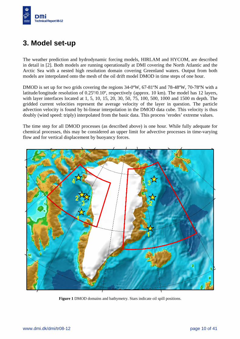
3. Model set-up The weather prediction and hydrodynamic forcing models, HIRLAM and HYCOM, are described in detail in [2]. Both models are running operationally at DMI covering the North Atlantic and the Arctic Sea with a nested high resolution domain covering Greenland waters. Output from both models are interpolated onto the mesh of the oil drift model DMOD in time steps of one hour. DMOD is set up for two grids covering the regions 34-0ºW, 67-81ºN and 78-48ºW, 70-78ºN with a latitude/longitude resolution of 0.25º/0.10º, respectively (approx. 10 km). The model has 12 layers, with layer interfaces located at 1, 5, 10, 15, 20, 30, 50, 75, 100, 500, 1000 and 1500 m depth. The gridded current velocities represent the average velocity of the layer in question. The particle advection velocity is found by bi-linear interpolation in the DMOD data cube. This velocity is thus doubly (wind speed: triply) interpolated from the basic data. This process ‘erodes’ extreme values. The time step for all DMOD processes (as described above) is one hour. While fully adequate for chemical processes, this may be considered an upper limit for advective processes in time-varying flow and for vertical displacement by buoyancy forces.

Figure 1 DMOD domains and bathymetry. Stars indicate oil spill positions.



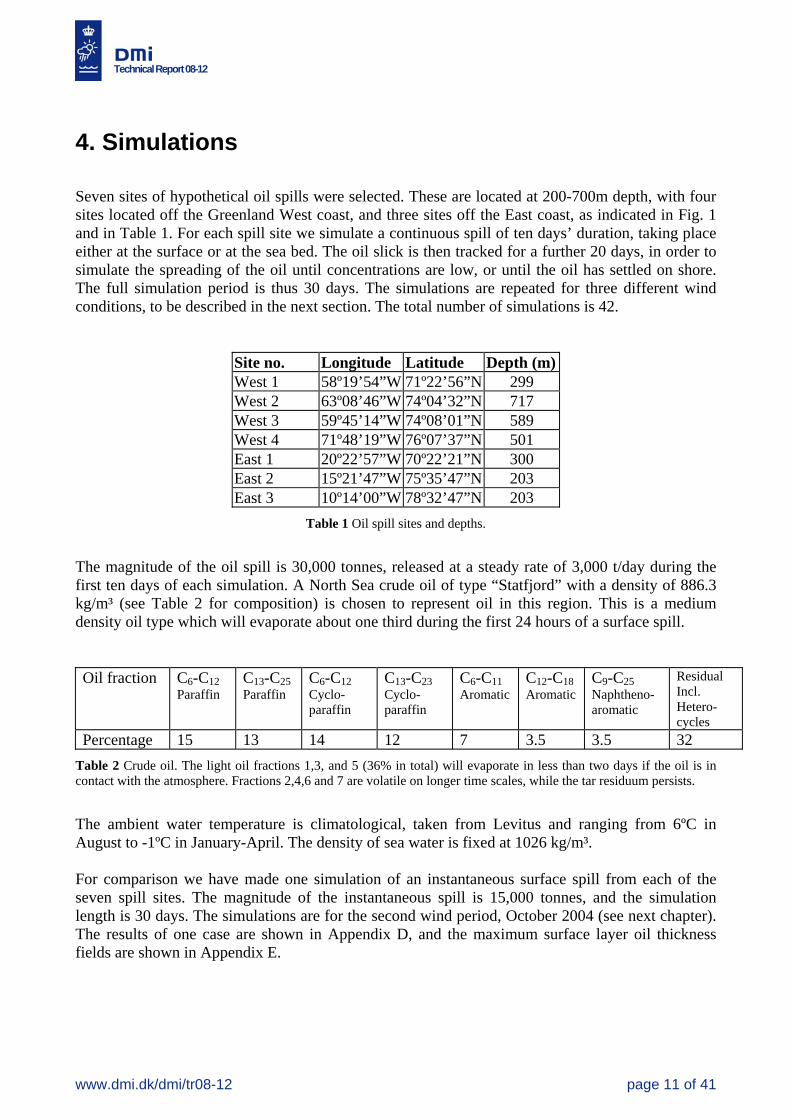
4. Simulations Seven sites of hypothetical oil spills were selected. These are located at 200-700m depth, with four sites located off the Greenland West coast, and three sites off the East coast, as indicated in Fig. 1 and in Table 1. For each spill site we simulate a continuous spill of ten days’ duration, taking place either at the surface or at the sea bed. The oil slick is then tracked for a further 20 days, in order to simulate the spreading of the oil until concentrations are low, or until the oil has settled on shore. The full simulation period is thus 30 days. The simulations are repeated for three different wind conditions, to be described in the next section. The total number of simulations is 42.

Site no. Longitude Latitude Depth (m)West 1 58º19’54”W 71º22’56”N 299 West 2 63º08’46”W 74º04’32”N 717 West 3 59º45’14”W 74º08’01”N 589 West 4 71º48’19”W 76º07’37”N 501 East 1 20º22’57”W 70º22’21”N 300 East 2 15º21’47”W 75º35’47”N 203 East 3 10º14’00”W 78º32’47”N 203

Table 1 Oil spill sites and depths.

The magnitude of the oil spill is 30,000 tonnes, released at a steady rate of 3,000 t/day during the first ten days of each simulation. A North Sea crude oil of type “Statfjord” with a density of 886.3 kg/m³ (see Table 2 for composition) is chosen to represent oil in this region. This is a medium density oil type which will evaporate about one third during the first 24 hours of a surface spill. Oil fraction C6-C12

Paraffin C13-C25 Paraffin

C6-C12 Cyclo- paraffin

C13-C23 Cyclo- paraffin

C6-C11 Aromatic

C12-C18 Aromatic

C9-C25 Naphtheno- aromatic

Residual Incl. Hetero-cycles

Percentage 15 13 14 12 7 3.5 3.5 32 Table 2 Crude oil. The light oil fractions 1,3, and 5 (36% in total) will evaporate in less than two days if the oil is in contact with the atmosphere. Fractions 2,4,6 and 7 are volatile on longer time scales, while the tar residuum persists.

The ambient water temperature is climatological, taken from Levitus and ranging from 6ºC in August to -1ºC in January-April. The density of sea water is fixed at 1026 kg/m³. For comparison we have made one simulation of an instantaneous surface spill from each of the seven spill sites. The magnitude of the instantaneous spill is 15,000 tonnes, and the simulation length is 30 days. The simulations are for the second wind period, October 2004 (see next chapter). The results of one case are shown in Appendix D, and the maximum surface layer oil thickness fields are shown in Appendix E.



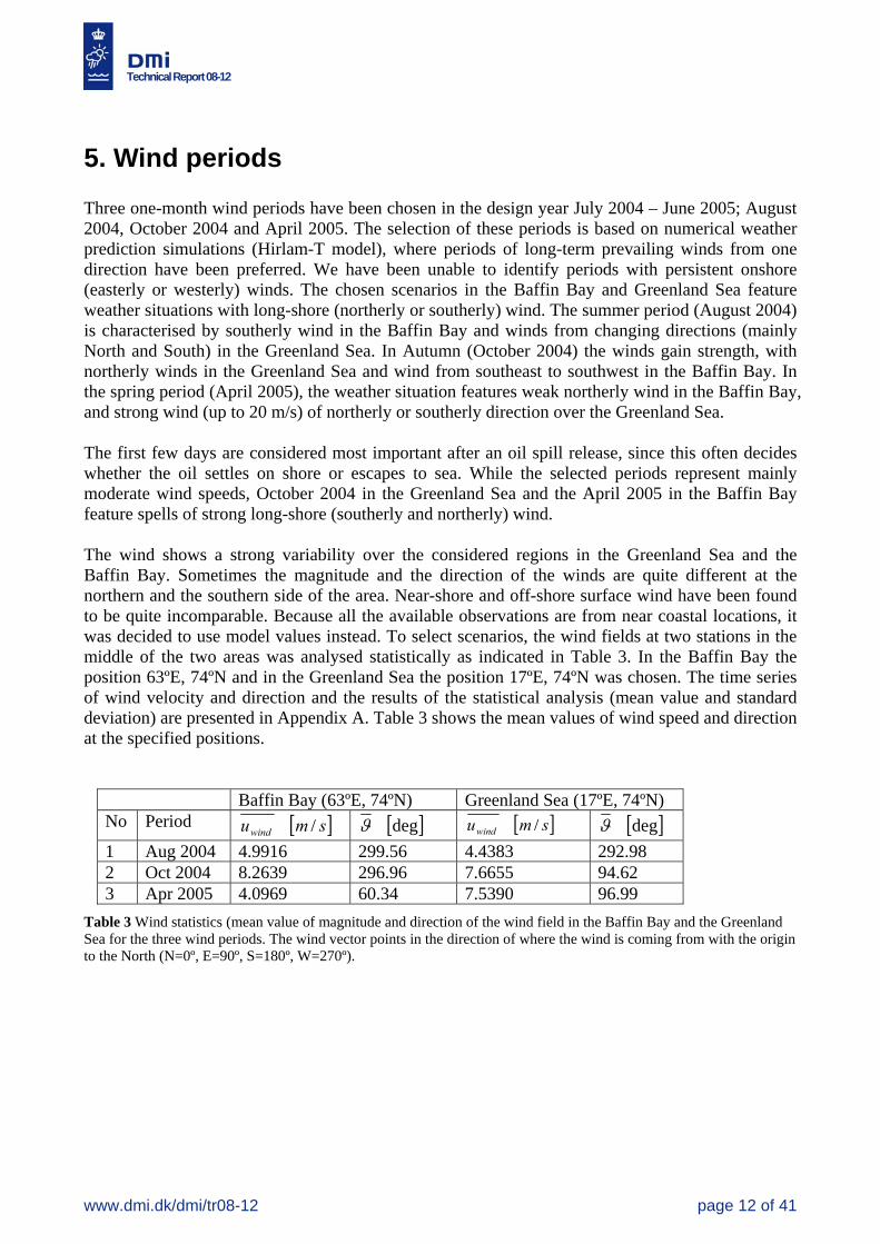
5. Wind periods Three one-month wind periods have been chosen in the design year July 2004 – June 2005; August 2004, October 2004 and April 2005. The selection of these periods is based on numerical weather prediction simulations (Hirlam-T model), where periods of long-term prevailing winds from one direction have been preferred. We have been unable to identify periods with persistent onshore (easterly or westerly) winds. The chosen scenarios in the Baffin Bay and Greenland Sea feature weather situations with long-shore (northerly or southerly) wind. The summer period (August 2004) is characterised by southerly wind in the Baffin Bay and winds from changing directions (mainly North and South) in the Greenland Sea. In Autumn (October 2004) the winds gain strength, with northerly winds in the Greenland Sea and wind from southeast to southwest in the Baffin Bay. In the spring period (April 2005), the weather situation features weak northerly wind in the Baffin Bay, and strong wind (up to 20 m/s) of northerly or southerly direction over the Greenland Sea. The first few days are considered most important after an oil spill release, since this often decides whether the oil settles on shore or escapes to sea. While the selected periods represent mainly moderate wind speeds, October 2004 in the Greenland Sea and the April 2005 in the Baffin Bay feature spells of strong long-shore (southerly and northerly) wind. The wind shows a strong variability over the considered regions in the Greenland Sea and the Baffin Bay. Sometimes the magnitude and the direction of the winds are quite different at the northern and the southern side of the area. Near-shore and off-shore surface wind have been found to be quite incomparable. Because all the available observations are from near coastal locations, it was decided to use model values instead. To select scenarios, the wind fields at two stations in the middle of the two areas was analysed statistically as indicated in Table 3. In the Baffin Bay the position 63ºE, 74ºN and in the Greenland Sea the position 17ºE, 74ºN was chosen. The time series of wind velocity and direction and the results of the statistical analysis (mean value and standard deviation) are presented in Appendix A. Table 3 shows the mean values of wind speed and direction at the specified positions.

Baffin Bay (63ºE, 74ºN) Greenland Sea (17ºE, 74ºN) No Period [ ]smuwind / [ ]degϑ [ ]smuwind / [ ]degϑ 1 Aug 2004 4.9916 299.56 4.4383 292.98 2 Oct 2004 8.2639 296.96 7.6655 94.62 3 Apr 2005 4.0969 60.34 7.5390 96.99

Table 3 Wind statistics (mean value of magnitude and direction of the wind field in the Baffin Bay and the Greenland Sea for the three wind periods. The wind vector points in the direction of where the wind is coming from with the origin to the North (N=0º, E=90º, S=180º, W=270º).



6. Sea ice conditions The three one-month periods may in short be characterized as follows; August is in the melting season, October is in the freezing season, April is in the ice season.

Baffin Bay Summer, August 2004: Sea ice covers the southern Baffin Bay close to the Baffin Island. It is rapidly melting, leaving an ice covered region behind, which is quickly reducing in size. The ice floe size and the ice concen-trations are quickly reducing. At the beginning of August, nearly half of the sea area is ice covered, leaving a strip of water open at the coast of Greenland. Although August is in the middle of the melting season, the ice covered part of the sea surface (ice concentration) reaches values of 60% to 80% at the Baffin Island. Towards the middle of August, these values sink to 50% to 70% and the ice covered region shrinks to a rather small zone in the middle of the Baffin Bay. At the end of August, the Baffin Bay is completely ice free. Autumn, October 2004: October 1st, the Baffin Bay is completely ice free. In mid-October, polar ice starts to move south-wards, and new ice starts to form in the northern Baffin Bay. The ice concentration reaches values of 50% to 70%. Towards the end of the month, the ice front moves more and more southwards and the ice thickness increases. Large parts of the Baffin Bay are then ice covered and the ice concentra-tion reaches values of 90%. Spring, April 2005: The Baffin Bay is completely covered with winter ice, reaching concentration values of 90% and more. In the southeastern Baffin Bay and straight at the Greenland coast this value drops to 70% and below. In the very North (Nares Strait), the ice concentrations and the percentage-ice-coverage of the sea surface drop down as well. There young ice and winter ice enters the Nares Strait from the North. This picture doesn’t change much over the whole of April.

Figure 2 Ice maps of the sea areas around Greenland. Left: summer 08.08.2004, centre: autumn 24.10.2004, right: spring 17.04.2005



Greenland Sea Summer, August 2004: At the beginning of August, the northwestern part of the Greenland Sea is covered with polar- and winter ice of a multitude of ice forms and concentrations ranging from dense ice (80% – 90%) in the North and at the coast to less dense (30% – 50%) towards the South and away from the coast. During August the ice is quickly melting and the ice front is retrieving, from approx. 70ºN at the beginning of August to approx. 75ºN at the end of the month. The ice concentration decreases to peak values of 50% – 70% and 10% – 30% in large areas. Autumn, October 2004: At the beginning of October the Greenland Sea is almost ice free. Only north of 75ºN and at the coast of Greenland there is a mix of polar, winter and young ice with medium to high concentration, highest to the north (60% – 80%) and lowest to the south (30% – 50%). Close to the coast there are places with a concentration of 80% – 90%. During the next weeks, the ice front is displaced south-wards towards 70ºN and both ice concentration and ice thickness are increasing. At the end of the month, nearly all the coastal area down to approx. 70ºN is covered with polar multi-year ice, and towards the South also with young ice. Spring, April 2005: The ice edge reaches all the way down the coast from the polar region to 65ºN. Generally The ice concentration decrease off-shore. The southeastern half of the Greenland Sea is completely ice free.



7. Results A total of 42 oil spill scenarios with continuous release have been simulated, with 7 release sites, 3 simulation periods, and 2 release depths. The basic output of each simulation is an hourly particle xyz location and property/status table. The particle property specifies its chemical composition, including water content. Its status includes particle age, shape, size, active/settled, located in-side/outside model domain, and others. Spill statistics are generated by averaging over all particles, and careful gridding, taking into ac-count the size and shape of each oil particle, results in oil concentration and slick thickness maps. As an example a case study of one of the simulations, release point West 1, wind period August 2004, is described in detail in Appendix B. Some specific and general features of the oil spill simulation output are discussed below.

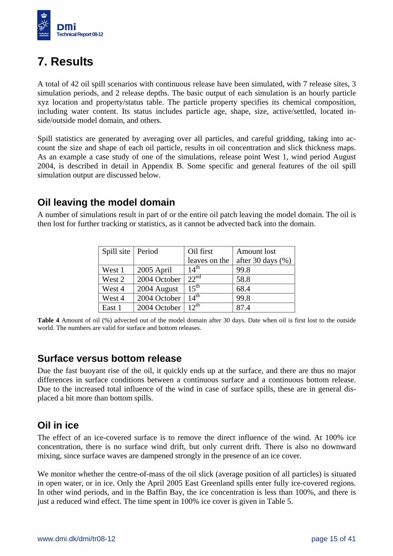
Oil leaving the model domain A number of simulations result in part of or the entire oil patch leaving the model domain. The oil is then lost for further tracking or statistics, as it cannot be advected back into the domain.

Spill site Period Oil first leaves on the

Amount lost after 30 days (%)

West 1 2005 April 14th 99.8 West 2 2004 October 22nd 58.8 West 4 2004 August 15th 68.4 West 4 2004 October 14th 99.8 East 1 2004 October 12th 87.4

Table 4 Amount of oil (%) advected out of the model domain after 30 days. Date when oil is first lost to the outside world. The numbers are valid for surface and bottom releases.

Surface versus bottom release Due the fast buoyant rise of the oil, it quickly ends up at the surface, and there are thus no major differences in surface conditions between a continuous surface and a continuous bottom release. Due to the increased total influence of the wind in case of surface spills, these are in general dis-placed a bit more than bottom spills.

Oil in ice The effect of an ice-covered surface is to remove the direct influence of the wind. At 100% ice concentration, there is no surface wind drift, but only current drift. There is also no downward mixing, since surface waves are dampened strongly in the presence of an ice cover. We monitor whether the centre-of-mass of the oil slick (average position of all particles) is situated in open water, or in ice. Only the April 2005 East Greenland spills enter fully ice-covered regions. In other wind periods, and in the Baffin Bay, the ice concentration is less than 100%, and there is just a reduced wind effect. The time spent in 100% ice cover is given in Table 5.



Spill site Spill depth Period Time spent in ice East 1 surface or bottom 2005 April 1st- 25th East 2 surface or bottom 2005 April 1st – 30th East 3 surface 2005 April 18th – 30th East 3 bottom 2005 April 20th – 30th

Table 5 Oil in ice, defined by position of centre-of-mass of the spill.

Drift The displacement of the oil (centre-of-mass) during 30 days of drift ranges from about 140 km to 460 km away from the release site. From the figures in Appendix C the effect of ice cover (of even less than 100% concentration) is seen. In the Baffin Bay, largest drift is found in October 2004 when the ice cover is at the minimum while August 2004 has slightly larger ice cover and weaker wind and thus smaller drift. April 2005 has only little oil drift due to the ice cover. On East Greenland the influence of ice is not as clear. In all cases the influence of the southward flowing East Greenland current is seen overlaid the influence of the wind. In this area October 2004 has largest oil drift, while August 2004 and April 2005 has smaller oil drift, probably due to calm weather in August 2004, and more ice in April 2005.

Spreading As indicated in section 2, the time dependency of the slick radius and area is calculated using a theoretical formulation for the radius increase. The spread depends on the time oil has resided in sea water. The slick area after 10 days, when all oil has been released, is 100-110 km², equivalent to a disc with a radius of 5.8-6.0 km. After 30 days, the slick radius has increased to about 22 km, and the slick typically covers an area of 1,400-1,500 km² of very irregular shape. In practice, the oil will form isolated patches within this area, with regions of high concentration interspersed with regions with no oil at a given time. This means that the area actually covered with oil is smaller than the indicated figured. The model gives no indication of how much smaller.

Downward mixing In calm weather the oil stays in a skin layer at the surface, and the oil is mixed down only during periods of strong wind. A maximum of about 12% of the oil is temporarily mixed down. The average mixing depth is 2 metres or less. The maximum mixing depth of an oil particle is 8-20 metres, depending on the site and the wind period. Two of the East coast April spills end up in ice-covered waters rather quickly, and are thus not mixed down.

Spill site August October AprilWest 1 11.7 15.6 12.2 West 2 10.4 19.7 9.9 West 3 9.9 15.0 9.5 West 4 11.7 12.3 8.3 East 1 16.3 19.4 11.7 East 2 11.0 17.4 0.0 East 3 12.3 18.5 0.0

Table 6 Maximum mixing depth (m). Only surface spills are considered.



Oil thickness A typical skin layer thickness after 10 days is 0.4-0.7 mm. After 30 days the mean skin layer thick-ness has decreased to 0.045-0.046 mm.

Oil composition The total water content converges towards two thirds for all oil particles, except when they settle very quickly (the particle composition is then fixed). All volatile components, about 36% of the oil evaporates during the first day or two after the oil has been released or has surfaced. The final volume is thus about double the spill magnitude.

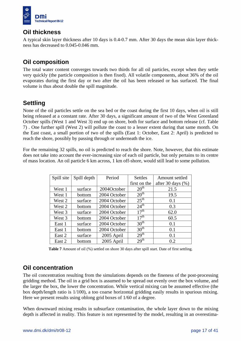
Settling None of the oil particles settle on the sea bed or the coast during the first 10 days, when oil is still being released at a constant rate. After 30 days, a significant amount of two of the West Greenland October spills (West 1 and West 3) end up on shore, both for surface and bottom release (cf. Table 7) . One further spill (West 2) will pollute the coast to a lesser extent during that same month. On the East coast, a small portion of two of the spills (East 1: October, East 2: April) is predicted to reach the shore, possibly by passing through or underneath the ice. For the remaining 32 spills, no oil is predicted to reach the shore. Note, however, that this estimate does not take into account the ever-increasing size of each oil particle, but only pertains to its centre of mass location. An oil particle 6 km across, 1 km off-shore, would still lead to some pollution.

Spill site Spill depth Period Settles first on the

Amount settled after 30 days (%)

West 1 surface 2004October 20th 21.5 West 1 bottom 2004 October 20th 19.5 West 2 surface 2004 October 25th 0.1 West 2 bottom 2004 October 24th 0.3 West 3 surface 2004 October 17th 62.0 West 3 bottom 2004 October 17th 60.5 East 1 surface 2004 October 30th 0.1 East 1 bottom 2004 October 30th 0.1 East 2 surface 2005 April 29th 0.1 East 2 bottom 2005 April 29th 0.2

Table 7 Amount of oil (%) settled on shore 30 days after spill start. Date of first settling.

Oil concentration The oil concentration resulting from the simulations depends on the fineness of the post-processing gridding method. The oil in a grid box is assumed to be spread out evenly over the box volume, and the larger the box, the lower the concentration. While vertical mixing can be assumed effective (the box depth/length ratio is 1/100), a too coarse horizontal gridding easily results in spurious mixing. Here we present results using oblong grid boxes of 1/60 of a degree. When downward mixing results in subsurface contamination, the whole layer down to the mixing depth is affected in reality. This feature is not represented by the model, resulting in an overestima-



tion of the concentration in the polluted layer. Furthermore, in real life a subsurface contamination decays rather slowly. In the model, the decay is represented by a sudden lift of the oil particle back to the surface, leaving a non-polluted layer behind. These two features should be kept in mind when applying model results. The highest concentration is found in the top metre of the water column, with a gradual decrease towards the sea bed. The highest value at any depth is found in the case of a bottom release, when the surface level momentarily exceeds 80,000 ppb. Layers below the maximum mixing depth are obviously only affected in case of a bottom release, and the maximum level is of the order of 10,000-20,000 ppb. Oil released at depth does not evaporate until surfaced, which accounts for the higher levels relative to surface releases. For surface releases, the oil concentration (40,000-50,000 ppb at the surface) drops off quickly with depth to disappear below 20m. The maximum skin layer thickness is about 2 mm. Maps of maximum oil slick thickness in the surface skin layer for each of the 42 simulations are found in Appendix C.

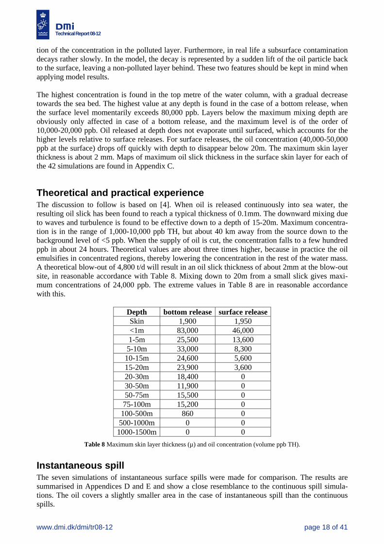
Theoretical and practical experience The discussion to follow is based on [4]. When oil is released continuously into sea water, the resulting oil slick has been found to reach a typical thickness of 0.1mm. The downward mixing due to waves and turbulence is found to be effective down to a depth of 15-20m. Maximum concentra-tion is in the range of 1,000-10,000 ppb TH, but about 40 km away from the source down to the background level of <5 ppb. When the supply of oil is cut, the concentration falls to a few hundred ppb in about 24 hours. Theoretical values are about three times higher, because in practice the oil emulsifies in concentrated regions, thereby lowering the concentration in the rest of the water mass. A theoretical blow-out of 4,800 t/d will result in an oil slick thickness of about 2mm at the blow-out site, in reasonable accordance with Table 8. Mixing down to 20m from a small slick gives maxi-mum concentrations of 24,000 ppb. The extreme values in Table 8 are in reasonable accordance with this.

Depth bottom release surface releaseSkin 1,900 1,950 <1m 83,000 46,000 1-5m 25,500 13,600 5-10m 33,000 8,300 10-15m 24,600 5,600 15-20m 23,900 3,600 20-30m 18,400 0 30-50m 11,900 0 50-75m 15,500 0 75-100m 15,200 0 100-500m 860 0 500-1000m 0 0

1000-1500m 0 0 Table 8 Maximum skin layer thickness (µ) and oil concentration (volume ppb TH).

Instantaneous spill The seven simulations of instantaneous surface spills were made for comparison. The results are summarised in Appendices D and E and show a close resemblance to the continuous spill simula-tions. The oil covers a slightly smaller area in the case of instantaneous spill than the continuous spills.



8. Conclusion A total of 42 one-month oil drift simulations of continuous spill have been carried out. The simula-tions result in hourly tables of position and properties of a cloud consisting of 1000 oil particles. Proper averaging results in bulk spill time series. A careful gridding technique is applied, resulting in oil slick thickness and concentration maps. By tracking all particles, the relative amount of oil settling on shore, and the shore affected, is calculated. The present text report gives only an over-all description of the simulation, while the detailed results are reported as data files. In the data files, both a coarse grid (1/60 degree or 1.6 km2) and a fine grid (1/120 degree or 0.4 km2) have been used. Both result in oblong grid cells, due to the convergence of the map projection towards the North Pole.



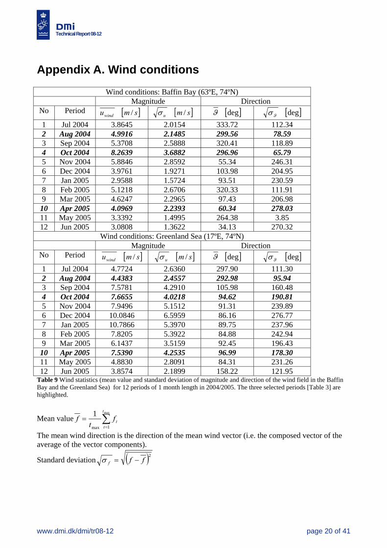
Appendix A. Wind conditions

Wind conditions: Baffin Bay (63ºE, 74ºN) Magnitude Direction

No Period [ ]smuwind / [ ]smu /σ [ ]degϑ [ ]degϑσ 1 Jul 2004 3.8645 2.0154 333.72 112.34 2 Aug 2004 4.9916 2.1485 299.56 78.59 3 Sep 2004 5.3708 2.5888 320.41 118.89 4 Oct 2004 8.2639 3.6882 296.96 65.79 5 Nov 2004 5.8846 2.8592 55.34 246.31 6 Dec 2004 3.9761 1.9271 103.98 204.95 7 Jan 2005 2.9588 1.5724 93.51 230.59 8 Feb 2005 5.1218 2.6706 320.33 111.91 9 Mar 2005 4.6247 2.2965 97.43 206.98 10 Apr 2005 4.0969 2.2393 60.34 278.03 11 May 2005 3.3392 1.4995 264.38 3.85 12 Jun 2005 3.0808 1.3622 34.13 270.32

Wind conditions: Greenland Sea (17ºE, 74ºN) Magnitude Direction

No Period [ ]smuwind / [ ]smu /σ [ ]degϑ [ ]degϑσ 1 Jul 2004 4.7724 2.6360 297.90 111.30 2 Aug 2004 4.4383 2.4557 292.98 95.94 3 Sep 2004 7.5781 4.2910 105.98 160.48 4 Oct 2004 7.6655 4.0218 94.62 190.81 5 Nov 2004 7.9496 5.1512 91.31 239.89 6 Dec 2004 10.0846 6.5959 86.16 276.77 7 Jan 2005 10.7866 5.3970 89.75 237.96 8 Feb 2005 7.8205 5.3922 84.88 242.94 9 Mar 2005 6.1437 3.5159 92.45 196.43 10 Apr 2005 7.5390 4.2535 96.99 178.30 11 May 2005 4.8830 2.8091 84.31 231.26 12 Jun 2005 3.8574 2.1899 158.22 121.95

Table 9 Wind statistics (mean value and standard deviation of magnitude and direction of the wind field in the Baffin Bay and the Greenland Sea) for 12 periods of 1 month length in 2004/2005. The three selected periods [Table 3] are highlighted.

Mean value ∑=

=max

1max

1 t

ttf

tf

The mean wind direction is the direction of the mean wind vector (i.e. the composed vector of the average of the vector components).

Standard deviation ( )2fff −=σ



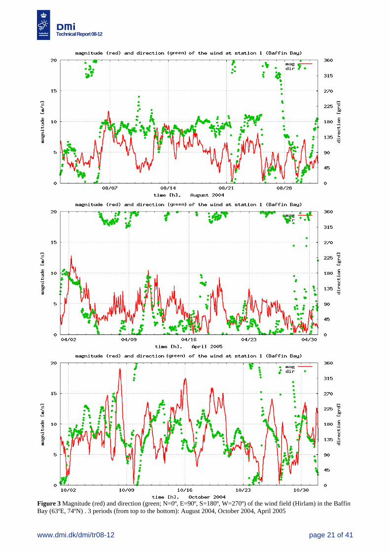
Figure 3 Magnitude (red) and direction (green; N=0º, E=90º, S=180º, W=270º) of the wind field (Hirlam) in the Baffin Bay (63ºE, 74ºN) . 3 periods (from top to the bottom): August 2004, October 2004, April 2005



Figure 4 Magnitude (red) and direction (green; N=0º, E=90º, S=180º, W=270º) of the wind field (Hirlam) in the Greenland Sea (17ºE, 74ºN) . 3 periods (from top to the bottom): August 2004, October 2004, April 2005



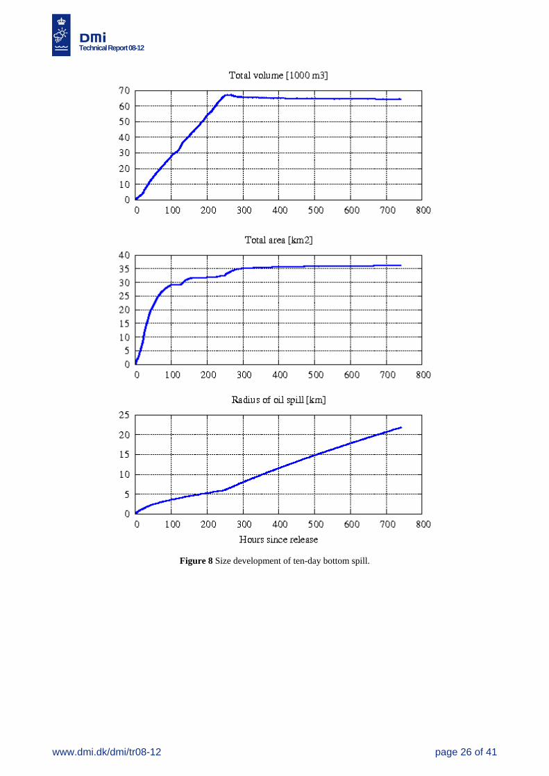
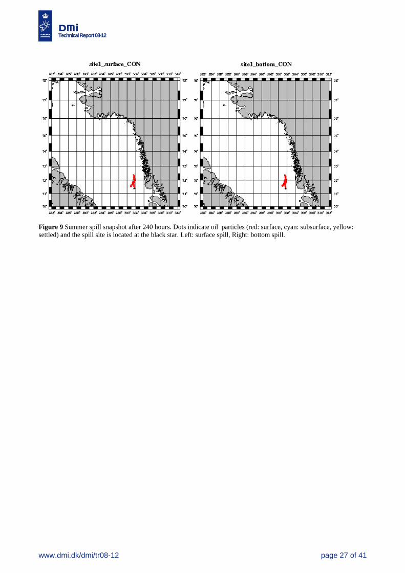
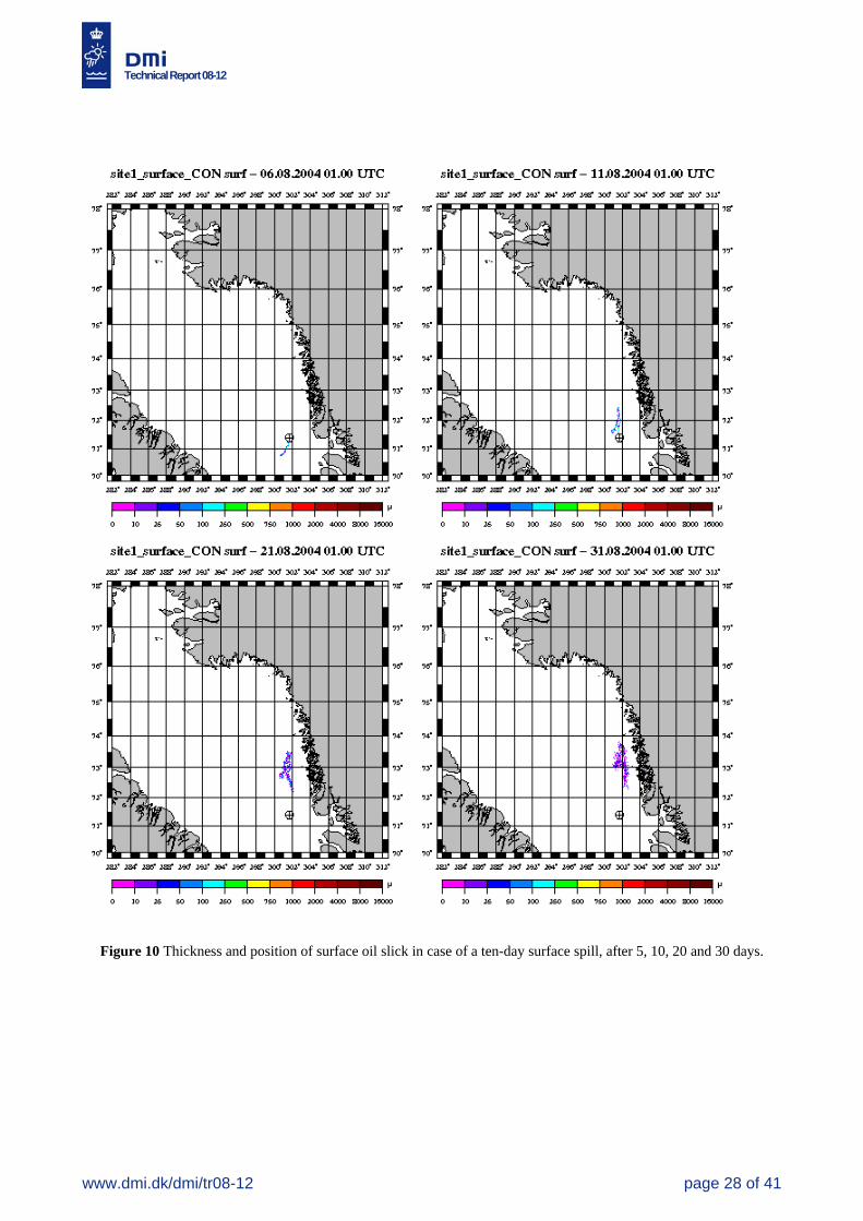
Appendix B. Case study In this section we single out one case for detailed description. The release point is West 1, located at 71º22’56”N, 58º19’54”W. We examine a one-month summer surface spill, lasting from August 1st-10th 2004 (period 1), and track it until the end of the month. The simulated oil statistics is shown in Figures 5 and 6, for a surface and a bottom (299 m depth) release, respectively. In none of the simulations does any oil settle on the sea bed or at the coast. The total water uptake converges toward two thirds, while 36% of the oil evaporates. These proc-esses roughly take place during the first two days. 60-65% of the oil ends up at the surface, even when released at large depth. Oil released at the sea bed quickly rises to the surface, and only a small amount is re-dispersed during periods with strong wind. The spill size is shown in Figures 7 and 8. The total volume and area grow approximately linearly with time during the first 10 days. The final volume is more than double the total amount of oil released (30t), even considering the loss of oil due to evaporation, due to the large uptake of sea water. This is important for oil combating purposes, since the oil-water mixture is rather stable, but less important for the oil concentration. The area affected by the release can be converted to a disc of 6 km radius after 10 days. Volume and area are a little larger for the bottom release than for the surface release. The spill particle distribution at day 10 is shown in Figure 9. The oil has drifted approximately 100 km to the north, maintaining distance to the Greenland coast. There is not much difference between a bottom and a surface release. As a result of the spill, the oil lies in a band extending from the source point northwards. Figure 10 shows the surface slick thickness after 5, 10, 20 and 30 days. The spreading of the oil results in a steady decrease of the thickness of the oil film (and thereby the potential for polluting the water masses below). After 10 days we still have values in the 0.1-0.25mm range, but after 20 days the level has fallen below 0.025mm everywhere, and below 0.01mm in much of the affected region. Assuming a mixing level of 10m, this corresponds to a potential oil concentration of 1,000 ppb TH. The spill results in a narrow band of oil, extending further and further away from the source point. The band broadens only very slowly, and towards the end of the simulation it is smeared out into a large patch of oil.



Figure 5 Oil statistics for ten-day surface oil spill.

Figure 6 Oil statistics for ten-day bottom off-shore oil spill.



Figure 7 Size development of ten-day surface spill.



Figure 8 Size development of ten-day bottom spill.



Figure 9 Summer spill snapshot after 240 hours. Dots indicate oil particles (red: surface, cyan: subsurface, yellow: settled) and the spill site is located at the black star. Left: surface spill, Right: bottom spill.



Figure 10 Thickness and position of surface oil slick in case of a ten-day surface spill, after 5, 10, 20 and 30 days.



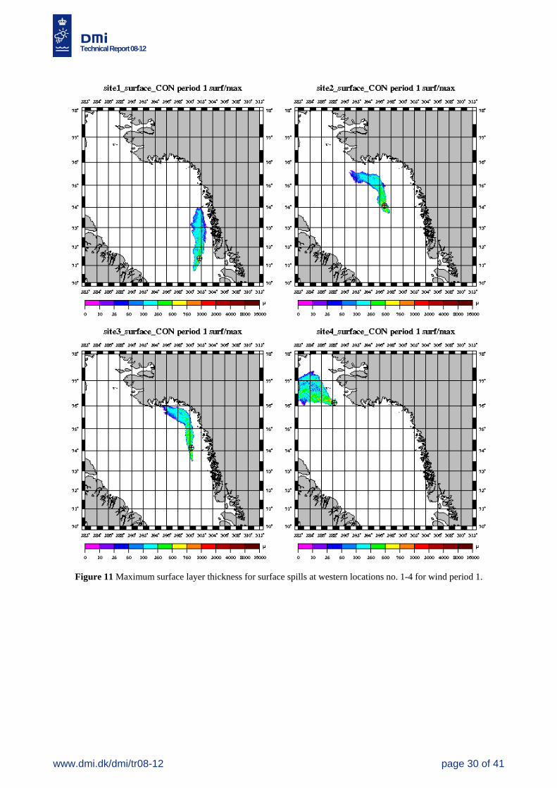
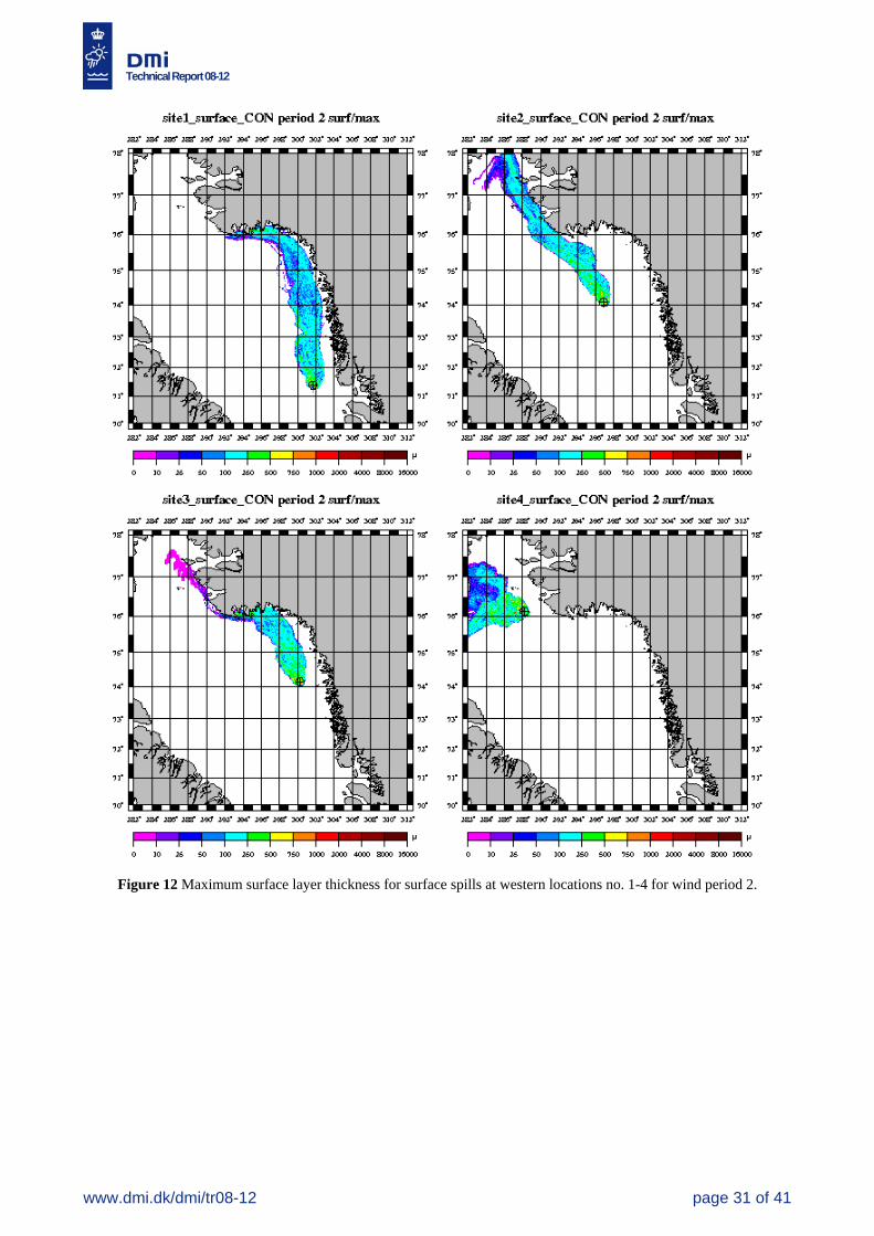
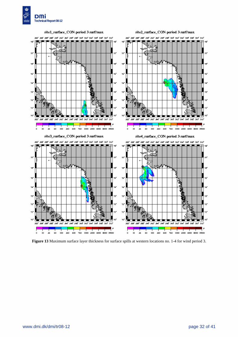
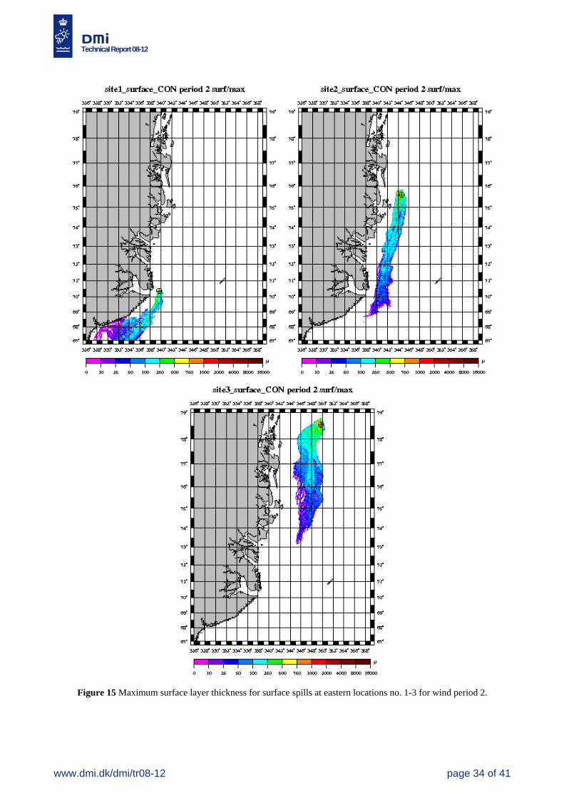
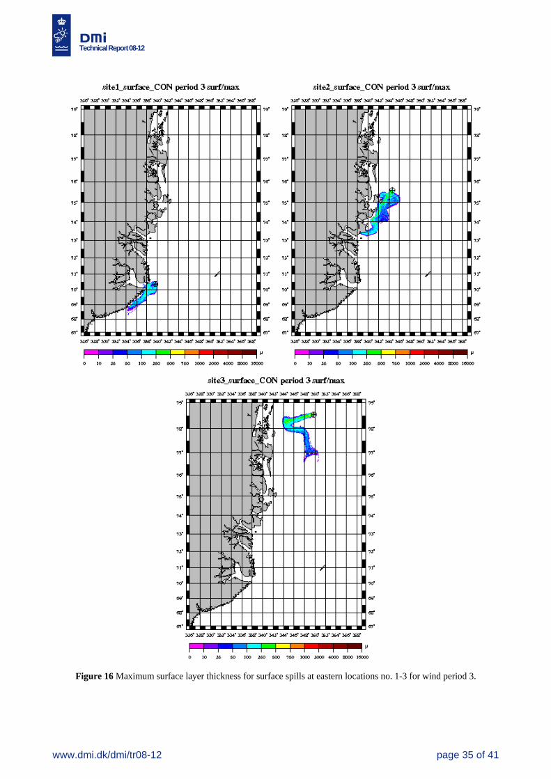
Appendix C. Maximum surface layer oil thickness For each of the 7 spill sites (4 western, 3 eastern), the maximum oil slick thickness in the surface skin layer attained at any time during the 30 days of simulation is mapped for each of the three wind periods. Only surface spills are shown. Bottom spills are very similar to the surface spills. Note that each figure does not represent the oil slick at a given time, but shows the area that at any time during the simulation has been covered by oil.



Figure 11 Maximum surface layer thickness for surface spills at western locations no. 1-4 for wind period 1.









Figure 14 Maximum surface layer thickness for surface spills at eastern locations no. 1-3 for wind period 1.









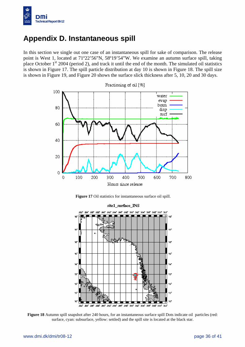
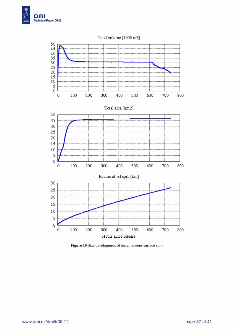
Appendix D. Instantaneous spill In this section we single out one case of an instantaneous spill for sake of comparison. The release point is West 1, located at 71º22’56”N, 58º19’54”W. We examine an autumn surface spill, taking place October 1st 2004 (period 2), and track it until the end of the month. The simulated oil statistics is shown in Figure 17. The spill particle distribution at day 10 is shown in Figure 18. The spill size is shown in Figure 19, and Figure 20 shows the surface slick thickness after 5, 10, 20 and 30 days.

Figure 17 Oil statistics for instantaneous surface oil spill.

Figure 18 Autumn spill snapshot after 240 hours, for an instantaneous surface spill Dots indicate oil particles (red:

surface, cyan: subsurface, yellow: settled) and the spill site is located at the black star.



Figure 19 Size development of instantaneous surface spill.



Figure 20 Thickness and position of surface oil slick in case of an instantaneous surface spill, after 5, 10, 20 and 30

days.



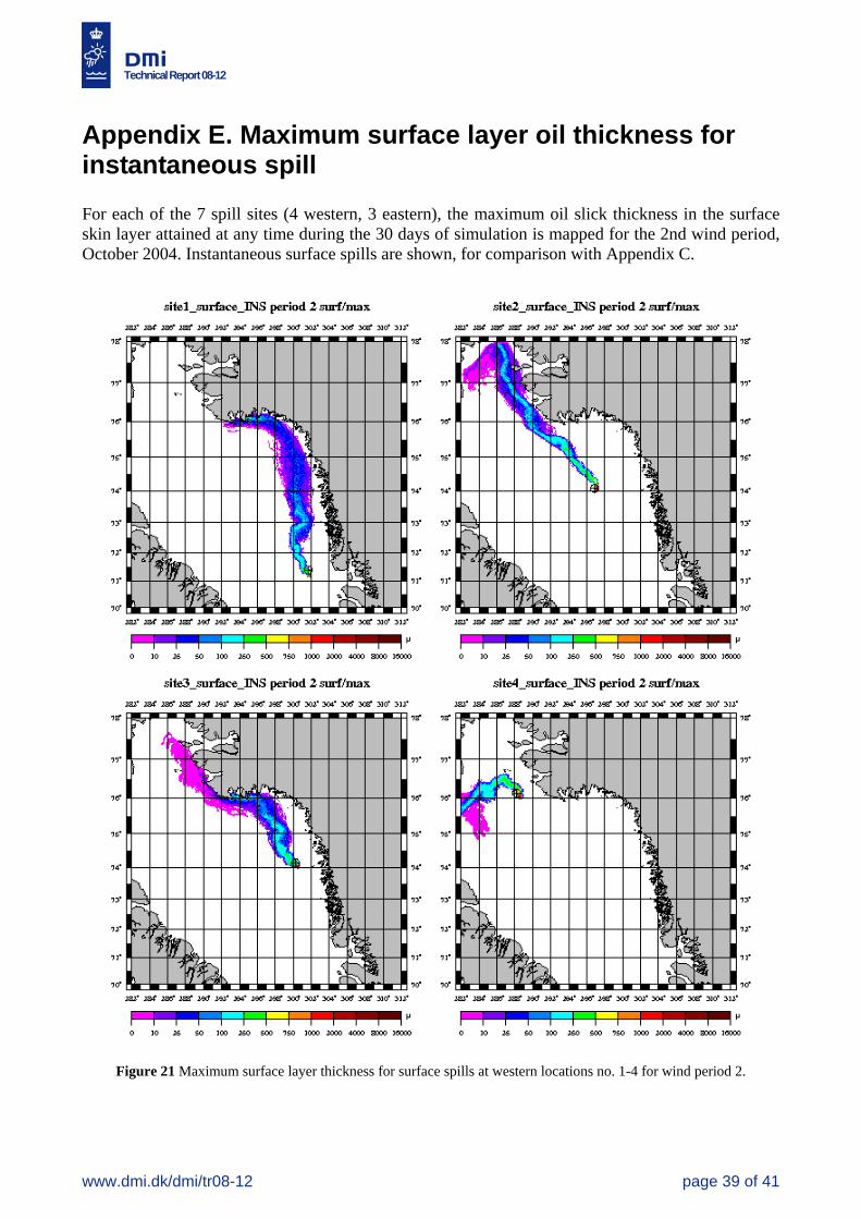
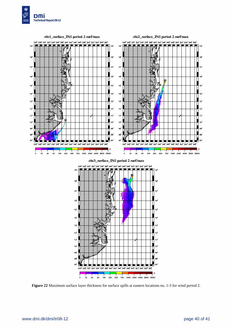
Appendix E. Maximum surface layer oil thickness for instantaneous spill For each of the 7 spill sites (4 western, 3 eastern), the maximum oil slick thickness in the surface skin layer attained at any time during the 30 days of simulation is mapped for the 2nd wind period, October 2004. Instantaneous surface spills are shown, for comparison with Appendix C.







References [1] J. W. Nielsen, N. Kliem, M. Jespersen and B. M. Christiansen, 2006: Oil drift and fate model-ling at Disko Bay. Techn. Rep. 06-06, Danish Meteorological Institute, Denmark [2] M. H. Ribergaard, N. Kliem and M. Jespersen, 2006: HYCOM for the North Atlantic Ocean with special emphasis on West Greenland Waters. Techn. Rep. 06-07, Danish Meteorological Institute, Denmark [3] S. Dick and K.C. Soetje, 1990: An operational oil dispersion model for the German Bight. Deutsche Hydrographische Zeitschrift, Ergänzungsheft Reihe A, nr. 16. Bundesamt Für Seeschiffahrt und Hydrographie, Hamburg. [4] J.A. Børresen, 1993: Olje på havet. Gyldendal. [5] B.M. Christiansen, 2003: 3D Oil Drift and Fate Forecasts at DMI. Techn. Rep. No. 03-36, Danish Meteorological Institute, Denmark. [6] Ø. Johansen et al., 2005: Simulations of oil drift and spreading and oil spill response analysis, Workpage 4 of project Arctic Operational Platform (ARCOP).

Previous reports Previous reports from the Danish Meteorological Institute can be found at:

http://www.dmi.dk/dmi/dmi-publikationer.htm

Documents

Technical Report 08-12 Oil drift and fate modelling off NE and NW