Bioimaging6 (1998) 138–149. Printed in the UK PII: S0966-9051(98)95425-9

TECHNICAL NOTE

Quantitative evaluation of lightmicroscopes based on imageprocessing techniques

L R van den Doel †, A D Klein , S L Ellenberger, H Netten,F R Boddeke , L J van Vliet an d I T Young

Pattern Recognition Group, Faculty of Applied Sciences, Lorentzweg 1,Delft University of Technology, NL-2628 CJ Delft, The Netherlands

Submitted 5 June 1998, accepted 25 June 1998

Abstract. In this note we will present methods based on image processing techniquesto evaluate the performance of light microscopes. These procedures are applied to threedifferent ‘high-end’ light microscopes. Tests are carried out to measure thehomogeneity of the illumination system. From these tests it follows that Kohlerilluminated images can have an exceedingly high amount of shading. Another resultfound from the illumination calibration is that traditional lamp housings are notdesigned to make fine-tuning easy. Next, the (automated) stage is considered. Severaltests are performed to measure the stage motion in thexy-plane and in the axialdirection to address accuracy, precision, and hysteresis effects. Finally, the entireelectro-optical system is characterized by measuring the optical transfer function (OTF)at wavelengths 400 nm, 500 nm, 600 nm, and 700 nm. The results of theseexperiments show that there is a consistent deviation from the theoretical OTF atwavelengths around 400 nm. The final conclusion is that modern light microscopesperform better than their five-to-ten-year-old predecessors.

Keywords: quantitative microscopy, calibration methods, digital image processing

1. Introduction

When using a (light) microscope as a quantitativeinstrument, careful calibration and testing are essentialto achieve proper results. A complete calibration of anadvanced microscope system would include, besides thecalibration of the microscope system itself as presented inthis note, a calibration of the charge coupled device (CCD)camera mounted on the microscope as well [1]. This studyconcentrates on the illumination system, the stage, and theelectro-optical system of a microscope. For fluorescencemicroscopy applications it is necessary that as much lightas possible is passed through the optical system and thatthe field-of-view is evenly illuminated. We have developedimage processing tools to calibrate the illumination systemin terms of the signal-to-noise ratio, shading, and theposition of maximum intensity. These measurements use aquadratic intensity profile as an approximation to the light

† E-mail address: richard@ph.tn.tudelft.nl

intensity distribution in the field of view. A series ofexperiments have been performed to measure the motioncharacteristics of the (automated) stage. The calibration ofthe stage is performed in terms of hysteresis (in both planarand axial directions), the focus position as a function ofthe stage position, and stability. The last two tests exploitfocus functions [2]. A complete calibration procedure of theautomatedz-axis, including axial resolution, can be foundin [3]. Finally, the electro-optical system is characterizedfor various objectives and for four test wavelengths in termsof the optical transfer function (OTF).

All experiments described in this note are performedon three different ‘high-end’ microscope systems. All threesystems will be described in section 2.1. In order to performall the experiments two different microscope test slideswere needed. These will be described in section 2.2. Alltest procedures, including the results and the conclusions,will be described in section 3.

0966-9051/98/030138+12$19.50c© 1998 IOP Publishing Ltd

Quantitative evaluation of light microscopes

2. Materials

2.1. Microscope systems

All calibration and test procedures are applied to threedifferent light microscopes: a Zeiss Axioskop (in ourlaboratory since 1993), a Zeiss Axioplan (1997), and aLeitz Aristoplan (in our laboratory since 1991). The ZeissAxioskop has a fully automatedxyz-stage (Ludl ElectronicsProducts Ltd, Hawthorne, NY, USA). The Zeiss Axioplancan be regarded as a completely digital microscope:objective revolver, reflector turret, and condenser aperture,for instance, can be adjusted by computer. The ZeissAxioplan used in this study, however, has only anautomatedz-axis. This implies that a number of procedurescould neither be implemented nor automated for thismicroscope. The Leitz Aristoplan has a fully automatedxyz-stage (Mac4000, Marzhauzer, Wetzlar, Germany). AKAF Photometrics Series 200 CCD camera can be mountedon both Zeiss microscopes. The array of the CCDelement contains 1317× 1035 pixels with a pixel size of6.8× 6.8 µm2. This camera is Peltier-cooled to−42◦C.Due to this cooling and a slow readout rate (500 kHz),this camera is photon limited. The characteristics ofthis camera in terms of signal-to-noise ratio are excellent[1]. This camera is connected via a NuBus interfaceto a computer. A Sony XC-77RRCE CCD camera ismounted on the Leitz Aristoplan. The CCD array contains756×581 pixels with a pixel size of 11.0×11.0 µm2, andthis camera is not cooled. The Sony camera is connectedto a computer via a Data Translation frame grabber. AnApple Macintosh Quadra 840AV computer takes care ofthe microscope control and the image acquisition. Boththe cameras and the microscopes can be controlled fromwithin the environment of an image processing package;this package is SCILImage (TNO Institute of AppliedPhysics (TPD), Delft, The Netherlands, e-mail address:scil@tpd.tno.nl).

2.2. Test slides

Two different test slides were used in this study. Forthe calibration of the epi-illumination an ALTUGLAS127.34000 Fluo green (Atochem Departement ALTUGLAS,4 cours Michelet - La Defense 10 Cedex 42-92091 Paris,France) was used. This slide is 75× 25 mm2 and about3 mm thick and is a homogeneous distribution of fluores-cent molecules embedded in a plastic matrix. As a result, auniform distribution of excitation light produces a uniformdistribution of fluorescent, emission light. The second testslide, which will be referred to as the HCM slide (Opto-LineCorporation, Andover, MA, USA) is used for various tests.This slide has a number of features.

• A grid of fiducial marks. The HCM slide containsfour rows labeled from A to D, each row containing a seriesof 12 fiducial marks labeled from A to L. The distance

AE AF AG AH AI

BE BF BG BH BI BJ

CE CF CG CH CI CJ

DE DF DG DH DI DJ

AJ

Figure 1. Part of the HCM slide. The top row, A, containstransparent density filters with squares and circles, the middlerow, B, contains opaque density filters with squares and circles,and the bottom row, C, contains empty density filters.Furthermore, the fiducial marks are shown labeled AE to DJ. AtCF and BG the fiducial marks are replaced by stage micrometers.

between two successive fiducial marks on a row is 4.5 mm.The distance between two successive fiducial marks ona column is 6.0 mm. The fiducial marks consist of twoperpendicular lines intersecting each other in their middle.The lines have a length of 0.2 mm and are 1µm thick. Thehorizontal lines of the fiducial marks along a row lie on thesame line. The same holds for the vertical lines. Two stagemicrometers have replaced the fiducial marks at ‘coordinatepositions’ BG and CF. The fiducial marks are used to checkthe alignment of the camera, and the slide with respect tothe stage. Furthermore, this grid of fiducial marks is usedto measure if thexy-plane of the stage is perpendicular tothe optical axis, and to test the motion characteristics of thestepper motors.• A row of optical density filters without pattern. These

filters are of size 3× 3 mm2, have transmission values inthe range 5%, 10%, . . . ,90%, and 100%, and are used forthe calibration of the trans-illumination.• Two rows of density filters with patterns. These

filters are of size 3× 3 mm2, their upper half containingsquares with sizes 10× 10 µm2 with an inter-squaredistance of 5µm and their lower half containing circleswith diameter 10µm with an inter-circle distance of5 µm. In row A the background pattern is transparentand the squares and circles have transmission values inthe range 5%, 10%, . . . ,90%, and 100%. In row B thebackground pattern is opaque and the squares and circleshave transmission values in the range 5%, 10%, . . . ,90%,and 100%. The two-dimensional patterns are used tomeasure the sampling density in pixelsµm−1.

A part of the HCM slide is shown in figure 1.

139

L R van den Doelet al

-400 -200 0 200 400

-400

-200

0

200

400

-400-2000 200400

-400-200 0 200 400

2600

2800

3000

3200

3400

100

-200 0 200

100

200

300

(a) (b) (c)

Figure 2. (a) The image of an empty field showing the shading, (b) the quadratic surface fit through the image, (c) the statisticaldistribution of the error, which is the distribution of the difference between the empty image and the quadratic surface. (The histogramis based on a reduced image (100× 100 pixels).)

2.3. Transmission filters

The characterization of the electro-optical system by meansof measuring the OTF(λ) requires near-monochromaticlight. For this purpose four narrow-bandpass interferencefilters are used, each with a bandwidth of 10 nm. The centerwavelengths of these filters are 400 nm, 500 nm, 600 nm,and 700 nm (Andover Corporation, Salem, NH, USA).

3. Procedures

In this section the variety of test procedures that usedigital image processing techniques will be described andthe results of these procedures applied to the differentmicroscope systems will be shown.

3.1. Illumination calibration

For fluorescence (epi-illumination) as well as for brightfield (trans-illumination) microscopy it is essential thatthe field of view is evenly illuminated. Furthermore, forfluorescence microscopy it is necessary that as much light aspossible is passed through the optical system. The seconddemand can be measured by computing the signal-to-noiseratio (SNR) of the total electro-optical system. The SNR isdefined as [1]:

SNR= 20 log

(µ

σ

)dB (1)

in which µ is the average brightness in the digital imageandσ is the standard deviation of the image brightnessesdefined by

σ 2 = 1

2

1

MN

M∑m=1

N∑n=1

(I1[m, n] − I2[m, n])2. (2)

In formula (2) it is assumed that both images consist ofM×N pixels. Since these images are not yet corrected forpossible non-uniform shading effects, two digital images,I1[m, n] and I2[m, n], are recorded and the pixel-to-pixeldifference is used to estimate the noise variance in theimages. Doing this, systematic spatial variations are‘subtracted out’. The average value can be estimated eitherby taking the average over theM ×N pixels in the imageor by taking the maximum brightness in the image. Theformer approach will be affected by the possible shadingand will, in general, lead to an underestimate of the average.The latter approach will be more reliable, but occasionallysubject to outliers or defective camera pixels.

In practice, it is difficult to achieve uniform illuminationas is illustrated in figure 2(a). The distribution of the lightintensity, however, can be assumed to have a quadraticform given by

Iqs(x, y) = β1+ β2x + β3y + β4xy + β5x2+ β6y

2. (3)

The approach in the illumination calibration is to fitthis light distribution through an empty image or a so-called white image as shown in figure 2(a). This fitis based on least-squares estimators. Given an imageI [m, n] it is possible to derive an analytical expression forthe parametersβ1, . . . , β6. In order to find least-squaresestimators for the parametersβ1, . . . , β6 the followingexpression must be minimized:

M∑m=1

N∑n=1

(I [m, n] − Iqs [m, n])2. (4)

The parameters then follow by differentiating thisexpression with respect to the parametersβ1, . . . , β6 andsetting the result equal to zero. This results in a set of sixequations, which look like (formula (4) differentiated with

140

Quantitative evaluation of light microscopes

respect toβ4)

β1S(m, n)+ β2S(m2, n)+ β3S(m, n

2)+ β4S(m2, n2)

+β5S(m3, n)+ β6S(m, n

3) =M∑m=1

N∑n=1

mnI [m, n] (5)

where

S(mp, nq) =M∑m=1

mpN∑n=1

nq (6)

is the product of two independent summations, for whichexpressions can be found in terms ofM and N . Thisset of equations can be written in matrix notationβ =A(M,N)I ′, with β = (β1, . . . , β6)

T , A(M,N) is a 6× 6matrix containing elements of the form of (6) and is just afunction of the image size (M×N pixels), andI ′ is a vectorof the form of the right-hand side of (5). The descriptionuntil now has been the standard procedure for quadraticregression [4]. Before inverting the matrixA(M,N),however, it is illustrative to have a closer look at itselements. Instead of summing over an asymmetric intervalfrom 1 to 2K+1 (2K+1 elements), one can also sum over asymmetric interval from−K toK (2K+1 elements). Thiscorresponds to a translation of the origin in the image fromthe upper left corner to the center of the image. Notice thefollowing:

K∑k=−K

ks = (−K)s + (−K + 1)s + · · ·

· · · + (K − 1)s +Ks = 0 s = 1, 3 (7)K∑

k=−Kks = (−K)s + (−K + 1)s + · · ·

· · · + (K − 1)s +Ks = 2K∑k=0

ks s = 2, 4. (8)

In (7) the terms disappear pairwise, whereas in (8) the termsappear exactly twice. The consequence of summing over asymmetric interval is that a number of elements ofA(M,N)become zero: each element withp or q odd. Forp or qeven, expressions can be found [5]. The inverse matrixA−1(M,N) now contains only ten non-zero elements. It isnow possible to compute the parametersβ1, . . . , β6.

The result of such a fit is shown in figure 2(b).Also shown in this figure is the histogram of the errorbetween the camera image and the fitted quadratic intensitydistribution.

Having fitted a quadratic intensity distribution, thehighest intensity(Imax) can be found by solving for theextremum of formula (3). The lowest intensity(Imin)can be computed along the border of the fitted intensitydistribution. Furthermore, the amount of shading in theimage and the root-mean-square (RMS) residual error canbe calculated. The shading gives information about thehomogeneity of the illumination in the image and the RMSis a measure for the quality of the fit. The amount of

Table 1. Results of the intensity check for microscopes andmodalities.

Microscope CV SNR(%) (dB)

Absorption Leitz Aristoplan 0.76 42.0Zeiss Axioskop 0.64 43.9Zeiss Axioplan 0.73 42.7

Fluorescence Leitz Aristoplan 1.80 34.9Zeiss Axioskop 1.14 38.8Zeiss Axioplan 0.74 42.7

shading in the recorded field of view can be calculatedfrom the highest and lowest intensities as follows:

shading= Imax − IminImax

× 100%. (9)

In the ideal situationImax is positioned in the center of theimage at coordinates(x = 0, y = 0). The position ofImaxcan be computed by manipulating (3). The goal of uniformillumination is to have as little shading as possible, i.e.Iminis as close as possible toImax .

The RMS is given as a percentage of the maximumintensity in the fit and is defined as

RMS= ((1/MN)∑M

m=1

∑Nn=1(I [m, n] − Iqs [m, n])2)1/2

Imax×100. (10)

Note that noise (e.g. photon noise and/or electronic noise)also has its effect on the RMS value. Using the positioningcontrols on the lamp housing it should be possible to centerthe maximum intensity and to improve the homogeneityof the illumination by reducing theshading as defined informula (9).

The calibration of the illumination starts with anintensity check for which the results are shown in table 1.The microscope lamps are centered and focused by usingthe Kohler procedures as described in the respectivemanuals of the microscopes. In this study 40× objectivesare used. The standard deviations,σ , as defined informula (2) are used for the calculation of the coefficient ofvariation(CV = σ/µ×100%) and are given as a percentageof the respective maximum intensities,µ, in each image.

After the intensity check a uniformity check isperformed and some typical results are given in table 2.Note that the shading percentages, as they are shownhere, should not be directly compared as they do notrepresent the same-size field of view. Two choices areavailable: one option is to standardize the size of thefield of view to compare the different microscopes. Thesecond option is to describe each microscope in termsof its specific shading. In table 2 the latter option isshown. In figure 3 an illustrative comparison is shown.The intensity distributions (given as a percentage of themaximum intensity) have about the same amount of shadingin the recorded images (1000× 1000 pixels) as defined

141

L R van den Doelet al

Table 2. Results of the uniformity check.

Microscope Image size Max. position Shading RMS(µm2) (%) (%)

Absorption Leitz Aristoplan 122× 122 (−1.20; 0.03) 4.52 1.96Zeiss Axioskop 172× 172 (−0.45; 4.66) 17.48 1.64Zeiss Axioplan 68× 68 (−0.43;−0.30) 16.31 1.71

Fluorescence Leitz Aristoplan 122× 122 (5.11;−1.20) 6.85 2.05Zeiss Axioskop 172× 172 (2.37;−3.03) 27.70 1.53Zeiss Axioplan 68× 68 (3.49;−0.63) 16.67 1.69

-500

50

-500

5050

75

100

-50 50

90

100

-500

50

-500

5050

75

100

-5000

500

-5000

50080

90

100

-500 500

90

100

-5000

500

-5000

50080

90

100

m pos. (pixels)

n pos. (pixels)

m pos. (pixels)

n pos. (pixels)

x pos. (µm)

y pos. (µm)

x pos. (µm)

y pos. (µm)

m pos. (pixels)

x pos. (µm)

0

0

Figure 3. The top-left intensity distribution in an image with 1000× 1000 pixels has about the same amount of shading as the top-rightintensity distribution. The left image corresponds to a field of view of 68× 68 µm2, whereas the right image corresponds to a field ofview of 172× 172µm2. When the image size is converted to a standard field of view of 100× 100µm2 as shown in the bottom-leftand bottom-right distributions, it is clear that the left distribution shows much more shading than the right distribution. The centerimages (top and bottom) show the value of the fitted surface along the lineIqs [m, n = 0].

in formula (9), but in a standardized field of view of100×100µm2 the left distribution has much more shadingthan the right distribution.

The RMS values in table 2 show that the quadratic fitto the shading is quite good. The value that is calculatedaccording to formula (10) can be regarded as the standarddeviation of the histogram shown in figure 2(c). Thestandard deviation in this histogram, which is composedof the error in the quadratic model plus the inherent noise

in the image, can be almost entirely attributed to the imagenoise as it is comparable to the noise value found in theSNR calculation.

As suggested above, measurements were also per-formed to follow the position of maximum intensity as thelamp was moved. This was achieved by turning the lamppositioning controls on the lamp housing and following theposition of Imax . A characteristic graph of these measure-ments is shown in figure 4.

142

Quantitative evaluation of light microscopes

-60 -50 -40 -30 -20 -10 10 20

10

20

30

40

50

60

-30 -20 -10 10 20 30

10

20

30

40

50

60

max. shading:

min. shading:

(a) (b)x-position

y-po

sitio

n

y-po

sitio

n

x-position

Figure 4. Effects of changing the lamp adjustment controls. The graphs show the movement of the position of the maximum intensityin the xy-plane when either the lateral (a) or the vertical (b) position is manually changed. The gray values of the arrows indicate theamount of shading.

3.2. Sampling density and component alignment

When measuring the sampling density in thex and ydirections it is important that the coordinate system ofthe camera and the pattern on the slide are aligned.Furthermore, measuring the stage characteristics requiresthat the coordinate system of the camera and the coordinatesystem of the stage are aligned. Three rotation angles canbe defined: first, the angle of the slide with respect to thecamera, denoted byαcam-sl , second, the rotation angle ofthe stage with respect to the camera,αcam-st ; and finally,the rotation angle of the slide with respect to the stage,αst-sl . By definition,

αcam-st + αst-sl = αcam-sl . (11)

Two rotation angles can be measured with respect to theframe of the camera:αcam-sl and αcam-st . The first anglecan be measured in a single image of one of the fiducialmarks of the HCM slide as shown in figure 5. First, thefiducial mark is skeletonized into a one-pixel thick objectwith one branch point. This branch point and its eight-connected neighbors are removed, resulting in two pairsof lines. Two straight lines are then fitted to the tworemaining pairs of lines of the skeleton using least-squaresestimators. Doing this the fiducial is completely definedby the subpixel intersection point of the two lines and bothslopes. The slopes of the lines define the rotation angle ofthe slide with respect to the camera. In order to measurethe rotation angle of the stage relative to the camera, themovements of the stage need to be related to the movementsof the intersection point of the fiducial mark in a series ofimages. The remaining rotation angle follows then fromformula (11). When the camera and the slide are aligned,the sampling densities in thex and y directions can bemeasured. For this purpose an area with circles or squaresof the HCM slide is used.

Figure 5. A 150× 150 image of part of a fiducial mark. Thewhite lines are the result of the skeleton operation. Thecomputed intersection point is(75.14, 85.74), and the slopes ofthe two lines are 0.000 34(θ = 0.02◦) for the horizontal line and−495.3 (θ = −89.88◦) for the vertical line. (The origin is in thetop left corner.)

First, after acquisition of an image with either squaresor circles, the objects connected to the border of theimage are removed. The coordinates of the centers ofgravity are computed for the remaining objects. Fromthe description of the HCM slide the distance betweentwo objects is known to be 15µm in both thex andy directions. From the list of coordinates the sampling

143

L R van den Doelet al

Table 3. Results of the sampling density measurements.

Microscope Objective Magnification Sampling density Nyquist frequencyrelay lens (pixelsµm−1) (λ = 400 nm)

(pixelsµm−1)

Leitz Aristoplan 40×/1.30/oil 1× 4.09(±0.1%) 13.0Zeiss Axioskop 40×/1.30/oil 1× 5.57(±0.02%) 13.0Zeiss Axioskop 40×/0.75/— 2.5× 14.11(±0.004%) 7.5Zeiss Axioplan 40×/0.75/— 2.5× 14.58(±0.007%) 7.5

density in both thex and y directions in pixelsµm−1

can be computed multiple times in a single image. Thissequence is repeated a (chosen) number of times and eachtime the stage is shifted a small random distance eitherautomatically or manually. The results are then averaged.This method is fast, because it uses a very simple algorithm,complete, because it measures the sampling density in bothdirections per image, and accurate, because the samplingdensity can be computed multiple times per image. Someof the results of this measurement procedure are givenin table 3. The measurements were performed with twodifferent relay lenses and two different 40× objectives.The sampling density values in both directions wereequal indicating ‘square pixels’. For a diffraction-limitedobjective the maximum spatial frequency can be determinedand the minimum sampling density (frequency) accordingto the Nyquist sampling theorem [6–8] is given by

fs > fNyquist = 4NA

λ. (12)

As can be seen in table 3, the combination oil-immersion objective, the 1× relay lens, and the camerado not lead to a sufficient sampling density. Both ofthe sampling frequencies are less than the critical Nyquistfrequency of 13.0 pixelsµm−1.

3.3. Stage characterization

3.3.1. Planar stage motion. One of the procedures forthe characterization of the stage is the measurement of theplanar xy motion of the stage. The basic procedure aswell as the results are described here. The measurementswere performed using a 40× objective. The goal of thisexperiment is to measure the hysteresis of the steppermotors. This is done by moving the stage back and forthover an increasing distance1x and measuring the errorbetween the defined distance and the measured distance.The experiment starts with one of the fiducial marks atthe left-hand side of an image. It is known that the finalmovement of the stage has been in the positivex direction.In that image the coordinates of the intersection point ofthe fiducial mark are determined. Then the stage is movedover a distance1x in the positivex direction such thatthe fiducial mark remains in the camera field of view. The

Table 4. Planar hysteresis for the Leitz Aristoplan and the ZeissAxioskop.

Microscope Hysteresis (blue) Hysteresis (red)(µm) (µm)

Leitz Aristoplan 1.13 1.27Zeiss Axioskop 0.39 0.35

subpixel crosspoint is again determined. Note that this is ahysteresis-free movement in the positive direction. Now thestage is moved in the negativex direction and once againthe crosspoint in the image is determined. A certain amountof hysteresis (in the negativex direction) is expectedin this movement. The algorithm is also performed inthe negativex direction to determine the hysteresis inthe positive direction. The results of these experimentsare shown in figure 6. Since the Ludl stepper motors(and the Marzhauser stepper motors) are not perfectlyidentical, these experiments should also be performed inthe y direction. The Zeiss Axioplan microscope is onlyequipped with a motor in the axial direction, thereforeno hysteresis measurements in the planar directions couldbe performed. In figure 6 the hysteresis can be seen asthe average distance between the blue and the red curve.The trend indicated by the dashed lines is the result of apositioning error. When the stage moves over a defineddistance of 1µm, it actually moves a little less. This erroris cumulative and the slope is 0.5 µm in 60µm or 0.8% inthe top graph of figure 6. Another feature that can be seenin figure 6 is the periodic behavior of the error. The periodof 20 µm equals the length of one full motor revolutionof the stepper motor. Similar graphs were obtained forthe Leitz Aristoplan. The measured planar hysteresis forboth directions for the two microscope systems is given intable 4. The hysteresis in the first column corresponds tothe blue curve in the top graph of figure 6, whereas thehysteresis in the second column of table 4 corresponds tothe red curve in the bottom graph of figure 6.

3.3.2. Axial position. By moving the stage along everyfiducial mark on the HCM slide and measuring the in-focusposition of every mark, az(x, y) surface can be found [3].Figure 7 shows the results for the three microscope systems.

144

Quantitative evaluation of light microscopes

20 40 60

-0.75

-0.5

-0.25

0.25

0.5

0.75

20 40 60

-0.75

-0.5

-0.25

0.25

0.5

0.75

mea

sure

d er

ror

in µ

m.

mea

sure

d er

ror

in µ

m.

∆x in µm.

∆x in µm.

∆x

∆x

−∆x

−∆x

Figure 6. For the Zeiss Axioskop with the Ludl motorized stage, the two graphs show errors with and without hysteresis. In the topgraph the initial position is always approached in the positivex direction. In the bottom graph the initial position is approached in thenegativex direction. The red curve is the error made in the positive direction (bottom graph, with hysteresis) and the blue graph theerror made in the negative direction (top graph, with hysteresis). The dashed lines show the trends.

A B C D E F G

A B C D0

20

40

60

A B C D E F G

A B C D0

20

40

60

A B C D E F G

A B C D0

20

40

60

18 mm 27 mm

a) Leitz Aristoplan b) Zeiss Axioskop c) Zeiss Axioplan

60 µ

m

x

y

z

Figure 7. Stage tilt(z) as a function of lateral position.z(x, y) surfaces found for the three microscope systems. For all three graphsthe z-range is 60µm.

The best results were found for the Zeiss Axioskop, but, ascan be seen in figure 7(c), thez(x, y) surface of the ZeissAxioplan is almost perpendicular to the optical axis of thesystem.

3.3.3. Axial hysteresis. To assess the hysteresis in thez direction we measured a focus function [2] twice, oncemoving the stage in the positivez direction and once inthe negativez direction. The results of this experimentare shown in figure 8. Each graph shows the two focusfunctions, F(z) against thez position, slightly shifted.This shift is caused by the hysteresis in the motor inthe axial direction. For two of the microscopes the shift

can be clearly seen; the shift is negligible for the ZeissAxioplan. This stage apparently incorporates a mechanismthat corrects for axial hysteresis.

3.3.4. Stability of the z-axis. If the focus functionhas been measured as a function of position,v = F(z),then the axial position relative to the in-focus position(z = 0) can be deduced from thez position asz =F−1(v). By acquiring images over a period of time withoutintentionally moving the stage, the stability of thez-axiscan be determined in the presence of mechanical vibrations,disturbances to the motor electronics, temperature changes,and gravity.

145

L R van den Doelet al

-5 -2.5 2.5 5

0.5

1

-5 -2.5 2.5 5

0.5

1

-5 -2.5 2.5 5

0.5

1

2.4 µm 1.6 µm

z-position

F(z

)

a) Leitz Aristoplan b) Zeiss Axioskop c) Zeiss Axioplan

Figure 8. Two focus functions, one moving upwards and one moving downwards, were measured for each microscope system. Thedistance between the in-focus positions is the axial hysteresis. The two focus functions almost completely overlap in (c).

2.5 5 7.5 10

0.1

0.2

0.3

0.4

0.5

30 60 90 120

F(z

)

z in µm t in min.

Figure 9. Results for a stability measurement on the Zeiss Axioskop. The left-hand side shows the focus functionF(z). The right-handside shows the focus value as a function of time. These focus values can be related to the distance from the in-focus position.

The Zeiss Axioskop gave reproducible results for thisexperiment. Typical results are shown in figure 9. TheLeitz Aristoplan and the Zeiss Axioplan did not. Overa period of 60 min the stage of the Zeiss Axioskopdropped about 5.7 µm or 96 nm min−1. To understand theimplications of this consider a microscope objective with adepth of focus of 1µm [9]. If a series of images is to beacquired for dynamical studies, then the images will remainin focus for up to 10 min.

3.4. Optical transfer function

The quality of images acquired through a properly adjustedmicroscope is inevitably limited by the lenses. The entireelectro-optical system of a microscope can be characterizedby means of its OTF. For an ideal circularly-symmetric,diffraction-limited objective the OTF is given by [10]

OTF(f ) =

(2/π)

(arccos(f/fc)− (f/fc)

√1− (f/fc)2

)|f | ≤ fc

0 |f | > fc(13)

wheref is the spatial frequency expressed in cycles perunit length, andfc is the cut-off frequency, representingthe maximum spatial frequency that can be passed throughthe lens [7, 11, 12]. The cut-off frequency is given by

fc = 2NA

λ. (14)

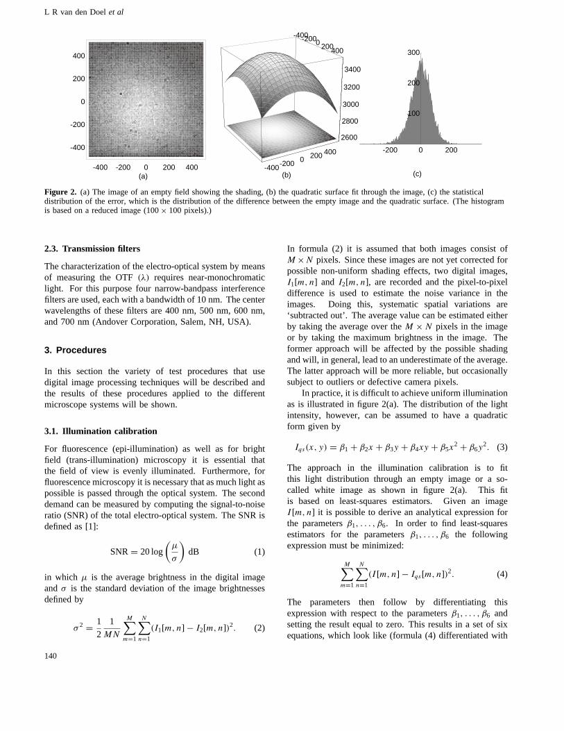
There are a variety of techniques for measuring the OTF.Some involve the use of ‘impulse-like’ objects, for examplemicrospheres, while others use bar patterns to determine acontrast modulation transfer function (CMTF), which canthen be transformed into the OTF [13–15]. Our procedurefor measuring the OTF requires an image of a ‘knife-edge’acquired with a known objective at a specific wavelength.A ‘knife-edge’ is simply a dark–white transition as shownin figure 10(a). It is essential that the image is sampledat a sampling frequency that meets the Nyquist criterionfrom formula (12). The first step in the procedure is tocorrect for shading in the image. This can be done eitherby the procedures described in section 3.1 or by a flat-field correction procedure. The latter procedure uses adark imageIdark[m, n], which represents the dark current.Furthermore, it uses a white imageIwhite[m, n], which is an

146

Quantitative evaluation of light microscopes

a)

b)

c)Figure 10. (a) The ‘knife-edge’ image. The red full curve is theintensity in grey values along a single line in this image. Theregion between the red dashed lines contains the dark–whitetransition. (b) A cubic spline interpolation algorithm with eightinterpolation points is applied to the dark–white transition in thetop image. The red curve shows the intensity along a row in theinterpolated image. (c) The derivative of the mid image iscomputed and the resulting set of PSFs is aligned to produce theline response.

empty image with only the illumination. This white imageincludes the dark image as well. The flat-field correction isthen based on the following equation:

If lat-f ield [m, n] = A I [m, n] − Idark[m, n]

Iwhite[m, n] − Idark[m, n](15)

whereA is a constant to scale the imageIf lat-f ield . Afterthe flat-field correction a 32-pixel-wide region around theedge is interpolated by a factor of eight using a cubic splineinterpolation algorithm [4] resulting in a 256-pixel-wideimage. The interpolated image is shown in figure 10(b).The result is convolved with a 7-pixel-wide 1-D derivative-of-Gaussian kernel withσ = 1.5 to obtain a smoothedestimate of the knife edge. This result can be regardedas the line response of the electro-optical system. Toobtain an improved estimate of the PSF the maxima arearranged line by line in the center column of the image,as shown in figure 10(c). These lines are then averagedcolumnwise to provide the 1-D PSF. The averaging overN lines improves the signal-to-noise ratio by a factor of√N . The Fourier transform of the PSF is the OTF. We have

measured the OTF for a collection of objectives for all threemicroscope systems and for four different test wavelengths.In figure 11 the OTFs are shown for three 40× objectives:one with NA = 0.75, and two withNA = 1.30. Thesampling densities of the objectives withNA = 1.30, asshown in table 3, are below the Nyquist frequency fromformula (12). However, the performance of these twoparticular objectives is so bad that the undersampling ofthe knife edge had no effect on the measurement of theOTF.

Several aspects of these curves are striking. First,the measured OTF cannot exceed the theoretical OTF, butseveral OTFs appear to do so. This is an artifact of thescaling of the curves. Each curve is scaled so that itsmaximum value is 1 and thus some OTFs are increasedin amplitude. In an ideal microscope lens system thereis no energy loss (photons) between input and output.In mathematical terms this translates to the conditionOTF(f = 0) = 1.

Second, the 40×/0.75 objective achieves almost idealperformance at the test wavelengthsλ = 500 nm,600 nm, and 700 nm. Atλ = 400 nm, however,no objectives perform near the diffraction-limited OTF:apparently, objectives are not corrected for wavelengths inthe deep blue (400 nm) part of the spectrum.

Finally, all of the OTFs have been plotted along thehorizontal axis in normalized units ofNA. This permitseasy comparison of each OTF per wavelength against theideal behavior, described by equation (13).

We suspect that the bad performance of the 40×/1.30objective is caused by prolonged use of this objectivefor multi-wavelength studies [16, 17]. This has led to adeterioration in the OTF performance of the lens.

147

L R van den Doelet al

NA/λ 2NA/λ

0.5

1

OT

F(f

)

Leitz Aristoplan 40x/1.30

NA/λ 2NA/λ

0.5

1

OT

F(f

)

Zeiss Axioplan 40x/0.75

NA/λ 2NA/λ

0.5

1

OT

F(f

)

Zeiss Axioskop 40x/0.75

NA/λ 2NA/λ

0.5

λ=400nm λ=500nm λ=600nm λ=700nm

1

OT

F(f

) Zeiss Axioskop 40x/1.30

theoretical OTF

Figure 11. OTFs for wavelengthsλ = 400 nm, 500 nm, 600 nm, and 700 nm for three microscopes and three objectives.

4. Conclusions

The purpose of this study was on the one hand to providea systematic approach, a methodology, for the evaluationof microscopes as quantitative imaging devices, and on theother hand to compare three specific microscope systems.The digital image processing techniques presented in thisnote are straightforward to implement and can be appliedto other scanning devices such as flatbed scanners. Withrespect to the comparison of microscopes, it is importantto understand that the measurements presented here are forone microscope of each type, one lens of each specific type,and one specific set of experiments. The Leitz Aristoplanmicroscope has been in constant use in our laboratory since1991, and the Zeiss Axioskop since 1993. These factorsshould be taken into account when weighing issues suchas illumination, planar and axial stage motion, and spatialresolution in terms of the OTF.

Acknowledgments

We would like to express our thanks to Dr Heinz Gundlachof Carl-Zeiss in Jena, Germany for making the ZeissAxioplan microscope available to us and to Dr Franc¸oiseGiroud of the Universite Joseph Fourier, Grenoble forproviding us with the HCM test slide. This workwas partially supported by the Netherlands Organizationfor Scientific Research (NWO) grant 900-538-040, theFoundation for Technical Sciences (STW) project 2987, theConcerted Action for Automated Molecular Cytogenetics

Analysis (CA-AMCA), the Human Capital and MobilityProject FISH, the Rolling Grants program of the Foundationfor Fundamental Research in Matter (FOM) and theDelft Inter-Faculty Research Center Intelligent MolecularDiagnostic Systems (DIOC-IMDS).

References

[1] Mullikin J C, van Vliet L J, Netten H, Boddeke F R,van der Feltz G and Young I T 1994 Methods for ccdcamera characterizationProc. SPIE Image Acquisitionand Scientific Imaging Systems (San Jose)vol 2173(Bellingham, WA: SPIE) pp 73–84

[2] Boddeke F R, van Vliet L J, Netten H and Young I T 1994Autofocusing in microscopy based on the otf andsamplingBioimaging2 193–203

[3] Boddeke F R, van Vliet L J and Young I T 1997Calibration of the automatedz-axis of a microscopeusing focus functionsJ. Microsc.186 270–4

[4] Press W H, Flannery B P, Teukolsky S A andVetterling W T 1998Numerical Recipes in C(Cambridge: Cambridge University Press)

[5] Mood A M, Graybill F A and Boes D C 1974Introductionto the Theory of Statistics(Singapore: McGraw-Hill)

[6] Oppenheim A V, Willsky A S and Young I T 1993Systemsand Signals(Englewood Cliffs, NJ: Prentice-Hall)

[7] Castleman K R 1996Digital Image Processing2nd edn(Englewood Cliffs, NJ: Prentice-Hall)

[8] Young I T 1989 Characterizing the imaging transferfunction Fluorescence Microscopy of Living Cells inCulture: Quantitative FluorescenceMicroscopy—Imaging and Spectroscopyvol 30B,ed D L Taylor and Y L Wang (San Diego, CA:Academic) pp 1–45

148

Quantitative evaluation of light microscopes

[9] Young I T, Zagers R, van Vliet L Jet al 1993 Depth-of-focusin microscopy8th Scandinavian Conf. on Image Analysis(Tromsø, Norway)(Tromsø: Norwegian Society forImage Processing and Pattern Recognition) pp 493–8

[10] van Vliet L J 1993 Grey-scale measurements inmulti-dimensional digitized imagesPhD ThesisDelftUniversity of Technology

[11] Born M and Wolf E 1980Principles of Optics6th edn(Oxford: Pergamon)

[12] Goodman J W 1996Introduction to Fourier Optics(New York: McGraw-Hill)

[13] Young I T 1983 The use of digital image processingtechniques for the calibration of quantitativemicroscopesProc. SPIE Applications of Digital ImageProcessingvol 397 (Bellingham, WA: SPIE) pp 326–35

[14] Young I T 1997 Calibration: sampling density and spatialresolutionCurrent Protocols in Cytometryed J P Robinsonet al (New York: Wiley)pp 2.6.1–2.6.14

[15] van der Voort H T M, Brakenhoff G J andJanssen G C A M 1988 Determination of the3-dimensional optical properties of a confocal scanninglaser microscopeOptik 78 48–53

[16] Netten H, Young I T, van Vliet L J, Vrolijk H,Sloos W C R and Tanke H J 1997 Fish and chips:automation of fluorescent dot counting in interphase cellnuclei Cytometry28 1–10

[17] Netten H, van Vliet L J, Vrolijk H, Sloos W C R,Tanke H J and Young I T 1996 Fluorescent dot countingin interphase cell nucleiBioimaging4 93–106

149