I.£'J1-.I

I

zI--

<

z

NASA TN D-1545

TECHNICAL

D-1545

NOTE

POWERINPUT TO A SMALLFLAT PLATE

FROMA DIFFUSELYRADIATINGSPHEREWITH APPLICATIONTO EARTHSATELLITES:

THESPINNINGPLATE

Fred G. Cunningham

Goddard Space Flight Center

Greenbelt, Maryland

NATIONAL AERONAUTICS AND SPACE ADMINISTRATION

WASHINGTON February 1963

https://ntrs.nasa.gov/search.jsp?R=19630003072 2018-07-29T13:06:13+00:00Z

4F

\

POWER INPUT TO A SMALL FLAT PLATEFROMA DIFFUSELYRADIATING SPHERE

WITHAPPLICATIONTO EARTHSATELLITES:THE SPINNINGPLATE

by

Fred G. Cunningham

Goddard Space Flight Center

SUMMARY

A general derivation is presented for the radiation from a uni-

formly radiating sphere incident on a small flat plate, sl_inning about

an axis not coincident with its normal. The results are presented as a

function of the separation of the bodies, the orientation of the plate, and

the orientation of the spin axis. In addition, a series of curves is given

which represents the power input from earth radiation to one side of a

spinning flat plate (averaged over a spin period) for a range of altitude

from 200 to 32000 km. These curves are based upon the assumption

that the earth is a uniform diffuse emitter radiating as a blackbody at a

temperature of 250°K.

CONTENTS

Summary....................................... i

INTRODUCTION.................................. 1

EXTENSIONOF THE METHODTO A SPINNINGPLATE ...... 2

DISCUSSION..................................... 9

RESULTS....................................... 10

ACKNOWLEDGMENT............................... 10

AppendixA- TheAverageIncidentPowerto a Flat PlateperSpinPeriodfor VariousAnglesa andb asa Functionof Altitude for theRange200< H < 3200 km ...... 11

Appendix B- The Average Incident Power to a Flat Plate per

Spin Period for Various Angles a and b as a Function

of Altitude for the Range 200 _< H _< 32000 km ...... 29

iii

POWERINPUT TO A SMALL FLAT PLATEFROMA DIFFUSELYRADIATINGSPHERE

WITHAPPLICATIONTO EARTHSATELLITES:THE SPINNINGPLATE

by

Fred G. Cunningham

Goddard Space Flight Center

INTRODUCTION

In a previous paper* (Part I) the power input to a stationary flat plate was calculated. The pres-

ent paper will apply these results to the problem of the spinning plate in order to determine the in-

stantaneous earth-radiated power incident upon the solar cell paddles associated with the various

satellites. This analysis does not consider any shielding of the paddles by other paddles or by the

body of the satellite itself.

In the previous paper we defined three cases for which the limits of integration were easily de-

terminable. These were dependent upon the value of the angle between the normal to the plate and

the earth-satellite line. For a spinning plate, however, this simplification is not possible since a

spinning plate whose axis of spin is not coincident with the normal to the plate defines a varying an-

gle between the normal and the earth-satellite line.

In general, a free rigid body whose axis of spin does not coincide with a principal axis exhibits,

to an external observer, a precession of the spin axis about the angular momentum vector and a pre-

cession of the axis of symmetry (in this case the normal) about the spin axis, so that both the axis of

symmetry and the axis of spin appear to precess about the angular momentum vector. However,

since we are considering plates attached to larger satellite bodies which usually spin about their

axis of symmetry (also a principal axis), the spin axis coincides with the angular momentum vector

and the net result is simply a precession of the normal about the spin axis. The main assumption

here is that the satel!ite's spin axis deviates no more than slightly from its axis of symmetry and

hence, possesses a negligible amount of precessional motion.

"Cunningham, F. G., "Power Input to a Small Flat Plate from a Diffusely Radiating Sphere with Application to Earth Satellites', NASA

Technical Note D-710 (Corrected copy), August 1961.

From the aforementioned paper, we can write the general expression for the instantaneous power

input to a stationary flat plate as

P - 7z {cos_cos_b + sin_sin¢cos¢)sine de de (1)

where:

A = the generalized emittance of the surface (or o_r4 for thermal radiation);

c = the emissivity of the surface of the radiating sphere;

a = the absorptivity of the plate;

A = the elemental vector area of the plate;

_b = the angle defining the position from the earth-satellite line of the radiating element ds on

the disk replacing the sphere;

¢ = the azimuthal designation of the element ds; and

), = the angle between the normal to the plate and the earth-satellite line.

The upper limit of the ¢integration is given by Cm = s in-l(1/H) where H is the earth-satellite vector,

and H is given in units of mean earth radii. The upper limit of the _ integration is determined by the

conditions governing the three previously mentioned cases:

(1) 0 -<_ -<(_/2-®o)

(2) (_/2 -%) < X < _/'2

(3) _/2 < x -<(_/2 +®o) .

In the first case the upper limit of _is _ for all ¢, and in the second case the upper limit is _ for

0 < ¢ < (n/2 - ;_). For the remaining portion of the second case and for all of the third case the upper

limit of ¢ is given by

- cos _ cos ¢cos_b = sin_, sine (2)

EXTENSIONOF THE METHODTO A SPINNINGPLATE

The flat plate whose spin axis ,., passes through the center of mass

but is not coincident with the normal A is shown in Figure 1,

where Figure 1--Geometry showingthe orientation oF the spinaxis and normal to the plate

II = the earth-satellite vector;

a = the angle between A and ,_;

b = the angle between [] and ,_.

We now define a new angle _ as the azimuthal angle of spin

of the plate about ,,; i.e., _, = d_/dt. Figure 1 shows the

zero value of the spin angle _ for the values of a and b

shown. In general the zero value of _ is defined when A Iies

in the H,,_ plane and >_is a minimum. Because of symmetry

we need not consider _ outside the range 0 < ¢ < _r. In ad-

dition, ,_ is assumed to be constant and of sufficient magni-

tude so that we need not consider a time weighted average

over the angle _ to determine the average power input over

the spin period, which is our ultimate goal.

w

*-"6

I

Figure 2--Unit sphere from which theangle ,k can be calculated

We shall consider the vectors ,_, H and A as unit vectors. Figure 2 shows the general orientation

of the spinning plate, where the ends of the vectors % H and A lie on the surface of a unit sphere.

With the above definitions, we can employ spherical trigonometry to determine 4. Clearly,

eos_ = cosacosb + sinasinbcos _. (3)

By inserting Equation 3 into Equation 1, we have

2AeaA

f_fc(cos acosb + sinasinbcos _) sin¢cos¢ d_ de

2AeaA C[ [1- (cosacosb + sina sinbcos _)211/2 cos_bsin2¢_ d¢ de (4)+ ---_---J+J+

The upper limit of the ¢ integration as given by Equation 2 becomes

and

-(cosacosb + sinasinbcos _)cosCOS_m : [1 - Coosacosb + ina inbcos (5)

However, as pointed out in the earlier paper, there are values of _ for which the argument of Equa-

tion 5 is greater than unity although _ lies within the proper bounds; for this situation ¢_ = _r. The

valuesof _bin questionare listed onpage2. A completediscussionof thevaluesof 4_and _ for which

Equations 5 and 6 are applicable will be presented subsequently.

Performing the ¢ integration of Equation 4 we have:

2AeaA fi_mP = _ - (cosacosb + sinasinbcos _)_b sin¢cos¢ de

2AE_A fo_+--_-- [1 - (cosacosb + sinasinbcos_)2]l/2sin_msin2¢ dqb (7)

In the regions where Equations 5 and 6 apply we have,

(cosacosb +sinasinbcos _) cos-If - (cos a cos b + sin a sin b cos _) cos ¢ ¢lsin q5cos Cd ¢[1 - (cos a cos b + sin a sinb cos _)2] ,/2 sin

+ [sin2¢- (cosacosb + sin a sin b cos _)2] l/_ sinCd¢ (8)

The values of _, which define the upper bounds of the regions of interest are _ = _/2 -¢_, rr/2,

7r/2 + ¢., for which the corresponding _ (for a given a and b) can be determined. These _ are defined

as follows:

sine,, - cosacosb

cos _1 = sin a sin b , for k = 7r/2 - ¢_ ; (9a)

- cos a cos bCOS _ _ = sinasinb , for k _/2 ; (9b)

¢o+cos u)c°s{2 = sinasinb , for x = 7r/2 +era " (9C)

Equation 8 gives the instantaneous power on a spinning flat plate as a function of the altitude

(from the upper limit of the ¢ integration), the angle between the instantaneous spin axis and the nor-

mal to the plate a, the angle between the instantaneous spin axis and the earth-satellite line b, and

the azimuthal angle of spin _ about the spin axis ,_. In the equation the arc cosine factor in the first

term and the square root factor in the second term arise from the ¢ integration; the first corre-

sponds to _ and the second to sin _. The arguments of these two factors contain functions of ¢,

and functions of a, b, and 4. These latter factors arise from the value of cos _, given by Equation 3.

In the previous paper the value of _ was assumed to be constant and calculations were made in the

appropriate range for various values of _,. In that case it was shown that for certain values of X the

range of integration over ¢ had to be divided into two subdivisions, for the first ¢. = _r and the abso-

lute value of the argument of the arc cosine factor is greater than unity, and for the second, ¢. is

less than_ andthecorrect valueis givenbythe arc cosinefactor. In fact, since _washeldcon-stant, it waspossibleto definethelimiting valueof the¢ integrationwhichdependedupon_, andhence,to breakthe integral into its parts-- only one of which contained the arc cosine factor as an

upper limit. However, in the present discussion we are considering the plate as it spins about an

arbitrarily oriented axis. Consequently, it follows from Equation 3 that _ is no longer constant in

time but varies with _ for the constant angles a and b. Then, in order to define the limiting values of

the ¢ integration we must make use of the dependence of _ upon _ where the corresponding limiting

values of _ are given by Equation 9.

As mentioned previously, a plate spinning about an axis not coincident with its normal (which is

a principal axis) exhibits a wobbly motion as the axis of symmetry (the normal) precesses about the

axis of spin. Before, we were able to hold _ within the range for which the power is incident upon

the side of the plate in question. The upper limit of this range is given by Equation 9c. When the

combination of the angles a, b, and 4 is such that _, as given by Equation 3, is greater than n/2 + ¢_

then the side of the plate under consideration is not visible from the earth, and the incident poweris zero.

Clearly we can define three distinct combinations of the angles a and b:

(1) _ -< (n/2-%) for 0 -< _ < n ; (10a)

(2) 0 < k <- (./2+¢m) for 0 < _ < _2 ; (10b)

(3) k > (n/2+%) for 0-< _ -<_ . (10c)

Equation 10c defines the situation with no radiation incident on the side of the plate in question; and

is of no further interest here. The condition defined in Equation 10a is the least complicated ex-

pression, integrable over _, for the power because the upper limit of the _ integration is _ for all

values of ¢ in the range 0 _< ¢ _< %. The general case is represented by Equation 10b where we in-

tend to imply that, over the range of 4 from 0 to _, the value of _ might be less than _/2 -¢_ for cer-

tain values of 4, greater than _/2-% but less than n/2 +¢_ for other values of _, and greater than

n/2 + % for still other values of _, or any other variation on the theme.

Equation 8 is the expression which must be integrated over ¢. It is identical to the equation in

Part I except that the corresponding expressions involving a, b, and _ for cos k and sin k are included.

Before attempting to calculate a given problem we must first examine the range of values of _ (given

by Equation 3) to determine the ranges of _ which are of interest. After the ¢ integration it then be-

comes necessary to average over 4, being careful to keep the appropriate range of _ coupled to the

proper expression.

For the case where Equation 10a applies, Equation 8 integrates to

sin -1 (I/H)

p = 2AeaA_ (eosaeosb + sinasinbcos{)sinCeosCd¢ , (11)

whichbecomes

A£c,AP H2 (cosacosb + sinasinbcos_) . (12)

Equation 12 is identical to the expression given as PI in Part I. We indicate the average over

by <P>_ which is

_ A_aA Ic sinasinb f; _I<P>_ H2 osacosb + vz cos_ d (13)

ACaA

H2 cos acosb (14)

The most general integral expression for the case of Equation 10b is:

,in -I (l/W)

P : 2A_,_A [ {cosacosb + slnastnbcos C) sin¢cos¢ d¢+a

./2-eo.-I 1_o.. _o. b + .in • +in b co. [1

+2A_aA _ (cosacosb + sinasinbcos _)sin¢cos¢ dqb

-0

0 ......

A sin -l ( 1/Vl)*_f ( ....... b+sinasinbcosr_}cos-lf_ -I ....... b + sina sinbcos _} cos¢

J.l,_[0.__<.................... {)] LO-- {....... b + sinasinbcos _}2Jt a sin+b)

2A-_ l "'i"-_ <lm)

+_l [ '+I"_¢+ - { ....... b + ,,ina,,i,+,bc'o,,++l_] ''+' sine d+

J./+ :[+o.-'¢....... ++.+.• .,. _+<..c+]

1,1n -j _l/_) }+_f2Aec_A [....... b ÷ sln . sinb co, _) cos'l _f ....-1 ....... b + sin a sinbcos {) cos¢

" J++-t< ....... _.+,+...+.b+o.+)-./+ t+tl - tcosacosb + *ir+.sir+,bcos_}m]t/+sin¢ slnCcosCd¢

lln -I /

+ f ........++,,+,+,,++o++00++,,+,,+,+,,,++J++.++ ira!. +ol b + .i...+. b +ol +) -=1:_

. i - cos a cos b

-cos a cos b --_cos-_ - cosacotb < _ < cos_ _ _g

(15)

Equation 15 integrates out exactly as Equations 21 and 35 of Part I except that we have replaced the

cosine )_ and sine ,\ factors by their equivalents in terms of _, b, and _.

Wenowhave:

H_(cosacosb + sinasinbcos_) 0 -< _ -< _1

+ Ae_'A{ 2 - sin-I [I - {cosacosb + sinasinbcos _)m] '12

I I _,f-(H 2 - 11 .....(..... osb + sinasinbyos{_)_

+ H_ \ ..... osb + slna sinbco$ _)cos _os; cosb + sina sinbcos _)_f,7

'_ '-it

A_o.AE C (H 2 - 1) / ] 1

/ I

+--7- sin-* .................... +- _)mr _ _ (cosacosb ÷ sinusinbcos_)i_ ) H 2 (ill _1) .....[i - H2(cosacosb + sinnsinbcos 2] ....

+ (eosncosb + sinasinbcos )cos '_-(H2 - l)'/x (cosacosb + sinasinbeos_)]k_

: -I.[ -+.... '1 - lcosacosb slnaslnbcos 1) ] '

(16)

where the expression in parentheses following certain terms in Equations 15 and 16 indicates the

range of _ over which the preceding terms are applicable. Because of the complexity of some of the

terms in Equation 16 the average over _ cannot be easily calculated in closed form so that this por-

tion of the problem will be left to the digital computer.

Equation 16 applies in its entirety only to the situation for which ?_does, indeed, have values

within all three regions defined by 0 -< ?_ -< (_/2 -era)' (_t2-¢_) <), -<_r/2, and _/2 < ?_ < (_1'2 +¢_) each

of which corresponds to a particular range of values of _ as _ goes from 0 to _. If ?_does not take on

values in all the regions for the entire range of _ certain modifications of Equation 16 must be made

which are pointed out subsequently. To determine which parts of Equation 16 to use and the corre-

sponding limits for any case, we must examine the range of _ for that case by checking its extremes.

Since A precesses about _ at a constant angle a, the extremes can be determined by considering the

cases when A lies in the H, ,.,plane; i.e., when _ = 0, 77. The only additional requirement is that ?_ < _.

In defining values of a and b it suffices that if we let b lie in the range 0 -5<b < _, we need only con-

sider a in the range 0 <- a < _r/2. For example, the situation represented by a = 100 °, b = 10 ° is

identically represented by the situation b = 170 °, a = 80 °. The direction of _, and consequently the

value of b, is always determined by the right hand rule. It also follows that interchanging the values

of a and b does not alter the problem. In addition, if we wish to determine the input to the other side

of the plate (called side 3) after having determined it for one side (called side c02 by the methods

outlined above, the extremes of the range of x for side fl can be easily calculated by subtracting the

limits for side a from 180 degrees. Then, once the extremes of ?_z are known, it is quite easy to

construct the corresponding values of a and b which, used in conjunction with Equation 3, will allow

for the determination of all the parameters of the new problem. For example, if a = 80 °, b = 170 °,

for side _, wehavethat 90° -<x <-110°;whereas70° <--x -< 90 ° for side _. The latter set corresponds

to b = 10 °, a = 80 ° or a = 10 °, b = 80 °.

We now outline the various possibilities of the general case represented by Equation 10b. But

first we shall make the following definitions for simplicity:

and

A _ ACaAH2 [cos a cos b + sin a sinb cos _] , (17a)

B - . - sin-l" 1 - (cosacosb * si--nasinbcos _}2] v2

1 cosacosb + sinasinbcos {)cos -1

+ H_ - (cosacosb + sina sinbcos _)_T--f

---i

-(H 2-1)v2 [1 - H2(cosacosb + sinasinbcos _)2],/_1.

_.1

Equation 16 can now be written in symbolic form:

(17b)

P -- A(O < _ <-_,) + B((_I < _ -<_') + B(_' < _ < _) (18)

The first step in any problem is to determine the range of x. We shall define three cases:

x < _/2 for all_; (19a)

x _ _/'2 for suitable values of _ in the range 0 5 ¢ 5 _;

x > ,/2 for all _.

(19b)

(19c)

In 19a the only value of C of concern is that for which X : 7/2-_ or _ = _x as given by Equation 9a.

If for a given value of t! the argument of the arc cosine in 9a is greater than +1 then X > (7/2 -¢= )

for all _ and Equation 16 reduces to

P -- B(0 -< _ < 7) • (20)

If, for a given value of H, the argument of the arc cosine in Equation 9a is greater than or equal to -1

but less than or equal to +1, so that Equation 9a defines the value of _ at which _, = (,/2-_=), then

Equation 16 becomes

P = A(0 -<(_< 5,) + B(_ I < _ <-"/T) (21)

However, if for a given value of H the argument of the arc cosine term in 9a is less than -1, then

_. < (77/'2-¢_) for all _ and Equation 16 becomes

P = A(O < _ < _) , (22)

which, when averaged over _, yields Equation 14 once again.

From 19b it immediately follows that _ can never be less than (_/2 -era) or greater than (n/2 +era)

for all _. Equations 9a and 9c define the limits of _ in question. In the preceding statement, the fact

that the value of the argument of the arc cosine in 9a can never be less than -1 and that the value of

the argument of the arc cosine in 9c can never be greater than +1 can easily be shown for any prob-

lem satisfying the conditions of 19b. If the argument of the arc cosine in 9a is greater than or equal

to -1 but less than or equal to +1 and the argument of the arc cosine in 9c is less than -1, Equa-

tion 16 reduces to

P : A(0 <- _ < _z) + B(_, < _ < _z) • (23)

If both the arguments of the arc cosines in 9a and 9c lie between +1 and -1 we then have Equation 16.

If the argument of the arc cosine in 9a is greater than +1 while the argument of the arc cosine of 9c

lies between +1 and -1, Equation 16 becomes

v = B(0 -< -< (24)

Finally, if the argument of the arc cosine in 9a is greater than +1 while the argument of the arc co-

sine in 9c is less than -1, Equation 16 reduces to

P : B(0 < _ -< _} • (25)

In 19c the only value of _ of concern is that for which £ = _/2 +¢mor _ = _2 as given by Equation 9c.

If the argument of the arc cosine in 9c is less than -1, x< (v/2 + era) for all _ and Equation 16

becomes

P = B(O < _ < _z) • (26)

If the argument of the arc cosine of 9c lies between +1 and -1, the value of _2 is defined and Equa-

tion 16 is

P = B(0 < _ < 42) • (27)

If the argument of the arc cosine of 9c is greater than +1 then )_ > (w/2 +era) for all _, and the corre-

sponding power input is zero.

DISCUSSION

Equation 16 is general and applies to any sort of diffusely radiating sphere. However, in the fol-

lowing calculations we are considering the diffusely radiating sphere to be the earth which radiates

as a blackbodyat a temperatureapproximatelyequalto 250°K.Thus

Ac :crTo4 , (28)

where e equals unity because of the equivalent blackbody approximation and a is taken equal to unity

in order to give the energy incident upon the plate. In addition, Equation 16 can be modified to give

directly the incident power to the plate as a function of the orbital position of the satellite by giving

H as a function of the orbital parameters and the azimuthal position of the satellite in orbit. This

can be done by utilizing the polar equation of an ellipse,

H = a(1- e _)1 + ecosv ' (29)

where 77is the angle giving the azimuthal position of the satellite from perigee, a is the semi-major

axis and e is the eccentricity. However, in the subsequent evaluations of Equation 16 this additional

information will not be included because the presence of the arc cosine factor in the equation renders

it almost impossible to write, in terms of the orbital parameters, the equation in closed form (after

averaging over _) so that not a great deal is to be gained unless we wish the computer to print out

the value for each orbital position.

So far we have only considered the case where the spin axis passed through the center of the

plate. However, it is easy to see that the dependence of _ on _ remains identical to that given by

Equation 3 for the case where a and b are defined as usual but the axis of spin is displaced from the

center of the plate. As long as this lateral displacement (usually half the width of a satellite) is

small in comparison to the distance of the plate from the surface of the sphere (which always ob-

tains for earth satellites) the previous analysis remains applicable.

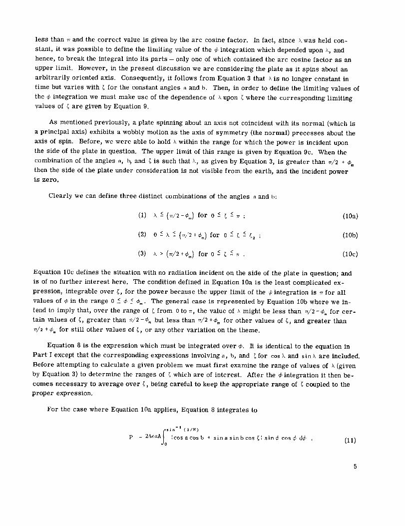
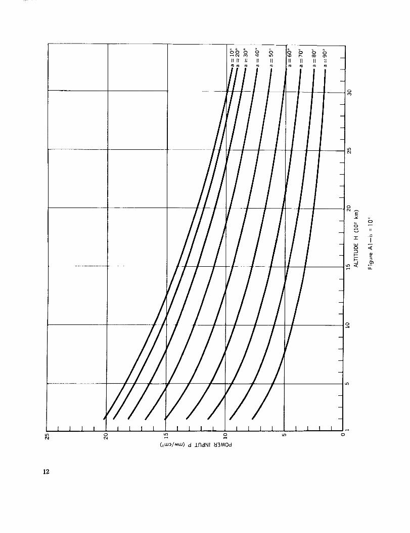
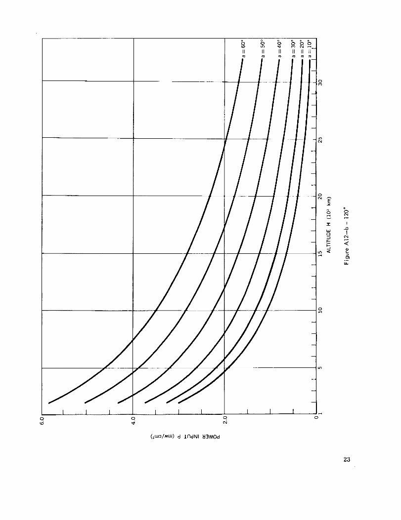
RESULTS

In the graphs that follow, the average incident power to the fiat plate per spin period is plotted as

a function of altitude above the surface of the earth for various values of the angles a and b. The situ-

ation occurring when b equals 0 or . results in k = a for all _ so that these values are not considered,

since the incident power for k = constant is readily available in Part I. This situation also applies

for a = 0 for which k = b = constant. The first 16 graphs apply for It in the range 200 _ H < 3200 km

(Appendix A), while the remaining graphs apply to the entire range 200 < H -<32000 km (Appendix B).

ACKNOWLEDGMENT

The author wishes to thank Mr. E. Monasterski, Goddard Space Flight Center, for the IBM 7090

computations.

10

AppendixA

The Average Incident Power to a Flat Plate per Spin Period for

Various Angles a and b as a Function of Altitude for the

Range 200 L H L 3200 km

11

II II II II III.D r... oo 0", _

II II II II

I I I I

Ill llili-

_ _ _

"r _ I- _, "2_ P- _

•-J I_

///--

///////'/#

I I I I I I l l i I I I I I I I

("d, ,.-i ,--i

(_.W3/MW) d J.ndNl }:l]MOd

12

0

bb 8 b

II II II II

///I

Illlj'/,/lil,

bbb8 III II II II

i :A -

I I 1 l i J I ! I I ILfl 0

i

/,/jj//jj/,///7,//'//

I I I I0

0

0

v

'1"

Q

ur) _

(_.,0/M,,,) d INdNI _3MOd

o

OC,4

_O

IC,4

O')

LL

13

t.O _ I_ OO 0".

II II II II II II

P

o

(:wo/,_w) d J_NdNI kl3MOd

14

/

1 I 1 I

//

/

///,,I 1 I 1 l 1

0,...4

I I

(:wo/,_w) d lndNI kl3MOd

0

0

0

v

7- _.0

_ Io ,<:ZI

- j_

ii

1

0

m

1

l l 1 10

15

....

I I I 1

I

II 11 I1 II II

iiiii

Ijr!rli

/

///'I

'1' 1 !

1 I

(_us0/Mw) d 1AdNI _13MOd

00")

I.n

0

,.-..i_ v

I

o

_ I.--

.,-,i

0

,.40

o

O

II

._0

f

I..,1_

16

I I I . I I ICO

(r.WO/MW) d ll7dNl _3MOd

I'_ CO

II II II II

0

m

u

C_

v

7-

r'_

<_,,-i

0

m

,-...i

O

oC_4O

II

_CI

I

o_IJ-

J

17

0

[ I I 1

(:w3/MW) d /fldNt _:JMOd

u

m

o

oE

v

"1-

-- w

w }'--

L¢) ',_

O

m

m

O

r_

ii

I

u_

18

I

O

/,

I I I

o o o

00 r_

o

(_W_/MW) d 1NdNI _3MOd

II I1

//

O

0

O

m

,..-t

1

0

1

Vl4

O

v

T

121

I--

F--

8

II

I

P

0-

19

0

O_

E,

II

/

/

I

0

00

I _ I I I 1

0 0 0

u_0

(:ua::,/,_ua) d lrtdNt _JMOd

m

oeo

w

m

o _.

,Iqv

2_

0,iq

0

¢,

0O-.

II

I0 _.

ii

20

0

21

Io o o o Io o o0 0 0 0 000 III II II II IIIIII

rv,II0

,!'/'l'ii

/ll/l!lI oI _g°

I!

"r ..Q

I _ .__

0

/"//t I

t_

,,'//

I I ..... 1O

0,,-i

t.fl

(_W:)/MCU) d .Lf'tdNI U]MOd

22

b b b _

II II II II II H

I j.,

g

// 2

Q0

..Q

I

.<

&u,_

0 0 00 ,--I

(zwo/Mw) d .l.IGdl',ll l:13MOd

23

0

1

11 II

i

!

//

1 i I I I ] I 1 1_ I I I I I I 1 1 10 0 0 0

0

v

"T

I.I

e_

I-1--

0

(_-uu01n_w) d J.NdNI _':lMOd

r-IO

a

OeO

I1

I

DO"J

u_

24

7bb

II

-1-

?,II

I I _ l I 1 I I 1 ! 1 I _ I I 1 [ 1 1 1 1

_ _ _ _ 0

(;:w3/,v,w) d J.NdNI _3MOd

I

ii

25

i

t-

o

O

2ic o

O

v II

"r

,,, ID ix")

l.--i

°mi1

i

ti'J

i I I I I l,

d d

0

(_lzi:_/Mu.i)d .ILf"ldNIt::l]MOd

26

0

0

o

e,.l

.-iv

"r

I.i.I

oi,--4

0..-4

II _ II '_ III I m l "_

0 0 0 0

d d 6(_,,,O/MWl d lndNI _]MOd

b"",0

II

.,aO

,I

ii

2'1

Appendix B

The Average Incident Power to a Flat Plate per Spin Period for

Various Angles a and b as a Function of Altitude for the

Range 200 L_ H _L32000 km

29

23

a = 10°'_..2O

a=30 _._ _ "_

E

O.

10

o

5

00.1 1

ALTITUDE H (10 :_ kin)

10 4O

F;gure Bl--b : 10 °

3O