Hydrol. Earth Syst. Sci., 23, 1567–1580, 2019https://doi.org/10.5194/hess-23-1567-2019© Author(s) 2019. This work is distributed underthe Creative Commons Attribution 4.0 License.

Technical note: Laboratory modelling of urban flooding:strengths and challenges of distorted scale modelsXuefang Li1, Sébastien Erpicum1, Martin Bruwier1, Emmanuel Mignot2, Pascal Finaud-Guyot3,Pierre Archambeau1, Michel Pirotton1, and Benjamin Dewals1

1Hydraulics in Environmental and Civil Engineering (HECE), University of Liège (ULiège), 4000, Liège, Belgium2LMFA, CNRS-Université de Lyon, INSA de Lyon, 69100, Lyon, France3ICube laboratory (UMR 7357), Fluid mechanics team, ENGEES, 67084, Strasbourg, France

Correspondence: Xuefang Li (xuefang.li@uliege.be)

Received: 11 September 2018 – Discussion started: 23 October 2018Revised: 11 February 2019 – Accepted: 24 February 2019 – Published: 18 March 2019

Abstract. Laboratory experiments are a viable approach forimproving process understanding and generating data for thevalidation of computational models. However, laboratory-scale models of urban flooding in street networks are oftendistorted, i.e. different scale factors are used in the horizon-tal and vertical directions. This may result in artefacts whentransposing the laboratory observations to the prototype scale(e.g. alteration of secondary currents or of the relative impor-tance of frictional resistance). The magnitude of such arte-facts was not studied in the past for the specific case of urbanflooding. Here, we present a preliminary assessment of theseartefacts based on the reanalysis of two recent experimentaldatasets related to flooding of a group of buildings and of anentire urban district, respectively. The results reveal that, inthe tested configurations, the influence of model distortionon the upscaled values of water depths and discharges areboth of the order of 10 %. This research contributes to theadvancement of our knowledge of small-scale physical pro-cesses involved in urban flooding, which are either explicitlymodelled or parametrized in urban hydrology models.

1 Introduction

Worldwide, floods are the most frequent natural disasters,and they cause over one-third of overall economic losses dueto natural hazards (UNISDR, 2015). Flood losses are partic-ularly severe in urban environments, and urban flood risk isexpected to further increase over the 21st century (Chen etal., 2015; Hettiarachchi et al., 2018; Lehmann et al., 2015;

Mallakpour and Villarini, 2015). In response, concepts suchas water-sensitive urban design, low impact development andthe sponge city model are rapidly developing (Gaines, 2016;Liu, 2016; Zhou et al., 2018). However, the design and sizingof measures aiming at enhancing urban flood protection re-quire accurate tools for risk modelling and scenario analysis(Wright, 2014).

Specifically, reliable predictions of flood hazard are a pre-requisite for supporting flood risk management policies. Thisincludes the accurate estimation of inundation extent, spa-tial distribution of water depth, discharge partition and flowvelocity in urbanized flood-prone areas, since these param-eters are critical inputs for flood impact modelling (Dottoriet al., 2016; Kreibich et al., 2014; Molinari and Scorzini,2017). State-of-the-art numerical inundation models benefitfrom increasingly available remote sensing data, such as laseraltimetry (e.g. Ichiba et al., 2018). Nonetheless, their valida-tion for urban flood configurations remains incomplete be-cause reference data from the field are relatively scarce and,to a great extent, inadequate (Dottori et al., 2013). Mostlywatermarks and aerial imagery are available, but they remainuncertain and insufficient (e.g. inadequate time resolution) inreflecting the whole complexity of inundation flows, espe-cially in densely urbanized floodplains. Additional informa-tion on the velocity fields and discharge partitions are nec-essary for understanding the multi-directional flow pathwaysinduced by the built-up network of streets and open areas,buildings, and underground systems (such as the drainagenetwork, (Rubinato et al., 2017), particularly under more ex-treme flood conditions. When available, pointwise velocity

Published by Copernicus Publications on behalf of the European Geosciences Union.

1568 X. Li et al.: Laboratory modelling of urban flooding

measurements remain limited in number due to the challeng-ing conditions for field measurement during a major urbanflood event (Brown and Chanson, 2012, 2013).

To complement field data, laboratory models may be aviable alternative, since they enable accurate measurementsof flow characteristics under controlled conditions. Recently,Moy de Vitry et al. (2017) used a full-scale lab experimentto explore the potential of video data and computer visionfor urban flood monitoring, but most laboratory experimentsof urban flooding were performed on reduced-scale models(Mignot et al., 2019). Existing lab studies representing ur-ban flooding at the district level provide data on street dis-charges and water depths (Finaud-Guyot et al., 2018) and, insome cases, also surface flow measurements (LaRocque etal., 2013). Few studies report point velocity measurementsfor urban flooding at the district level (Güney et al., 2014;Park et al., 2013; Smith et al., 2016; Zhou et al., 2016), whiledetailed velocity measurements are generally available onlyfor more local analyses (e.g. at the level of a single manhole;Martins et al., 2018).

Laboratory-scale models consist of replicating a full-scaleconfiguration (also called prototype) at a smaller scale. Thescale factor of such a model is defined as the ratio Lp/Lmbetween a characteristic length Lp in the prototype and thecorresponding characteristic length Lm in the model (Novak,1984). The design of scale models is based on the similar-ity theory, which states that the ratio between the dominat-ing forces governing the flow should remain the same in themodel and in the prototype. For free surface flows, Froudesimilarity is generally used; the ratio between inertia forcesand the gravity are kept identical in the model and in the pro-totype. This implies that the Froude number Fm in the modelremains the same as the Froude number Fp in the prototype,where the Froude number is defined as F = V/(gH)0.5, withV as a characteristic flow velocity (ms−1), g as the gravityacceleration (ms−2) and H as a characteristic water depth(m).

Caution must be taken when interpreting observationsfrom laboratory models because not all the ratios of forcescan be kept the same in the prototype and in the model. Forinstance, when the Froude similarity is applied, the ratio be-tween inertia and viscous forces may vary between the pro-totype and the model. This may result in so-called scale ef-fects, which are artefacts arising from the reduced size of themodel compared to the real-world configuration due to gov-erning non-dimensional parameters (i.e. force ratios) whichare not identical between the model and its prototype (Heller,2011). This may include alteration of the flow regime (lam-inar or transition, instead of complete turbulent), of the rela-tive importance of friction resistance or of 2-D and 3-D flowstructures.

The ratio between inertia and viscous forces is expressedthrough the Reynolds number: R = 4RHV/ν, with RH as acharacteristic value of the hydraulic radius (ratio between theflow area and the wetted perimeter, in metres) and ν as the

kinematic viscosity of water (m2 s−1). According to Froudesimilarity and without distortion (see Sect. 2.1), R scaleswith the power −3/2 of the scale factor of the model. There-fore, the magnitude of the scale effects tends to be magni-fied when a larger scale factor is used. Still, for large enoughReynolds numbers (i.e. sufficiently turbulent flow) both onthe prototype and in the model, the impact of the scale ef-fects remains limited. For modelling rivers and flood plains,Chanson (2004) recommends keeping the Reynolds numberabove 5000 for the lowest flow rate and using scale factorsbelow 25–50. These recommended values are mainly experi-ence based, but they were never ascertained for urban flood-ing models.

One process which is particularly complex to represent in-scale models of urban flooding is the frictional resistance.Given that smooth material is generally used to construct thebottom and the walls of these models, there are two compet-ing effects (lower Reynolds number in the model comparedto the prototype but also lower relative roughness) which, ingeneral, hamper a definite prediction of whether frictional re-sistance is overestimated or underestimated compared to theprototype. This issue is further discussed in Sect. 5.1.

Recently, urban flooding in street networks has been anal-ysed experimentally in laboratory set-ups that aim to repre-sent inundation flow across a whole urban district. To coveran entire urban district in a laboratory, while keeping theReynolds number reasonably high and limiting the measure-ment errors, distinct scale factors have been used along thehorizontal and the vertical directions, leading to so-calleddistorted scale models. This type of model was used pre-viously for various applications (e.g. fluvial morphodynam-ics), but its use for urban flooding studies is relatively new(Finaud-Guyot et al., 2018; Güney et al., 2014; Smith et al.,2016). While scale effects in general were investigated in thepast for a range of configurations, such as the experimen-tal representation of impulse waves (Heller et al., 2008) orthe hydraulics of piano key weirs (Erpicum et al., 2016),the specific artefacts arising from the model distortion werehardly studied, particularly not for experimental models ofurban flooding. Given the overwhelming importance of ur-ban flooding, the present paper focusses specifically on theeffects of model distortion in laboratory modelling of urbanflooding at the district level. It presents a reanalysis of tworecent experimental datasets (Araud, 2012; Velickovic et al.,2017) to find out to which extent a strong distortion of anentire urban district model affects the observed water depthsand flow partition in-between the streets.

Section 2 provides background information and details themotivations of the study. The considered datasets and themethodology are described in Sect. 3. The results are pre-sented in Sect. 4, and implications thereof are discussed inSect. 5. Finally, conclusions are drawn in Sect. 6.

Hydrol. Earth Syst. Sci., 23, 1567–1580, 2019 www.hydrol-earth-syst-sci.net/23/1567/2019/

X. Li et al.: Laboratory modelling of urban flooding 1569

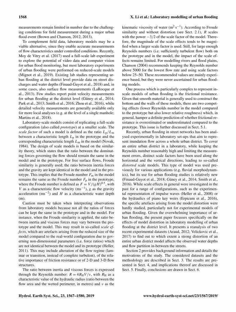
Table 1. Recent laboratory experiments of urban flooding at the district level.

References Prototype Model spatial Horizontal Vertical Reynolds numberspatial extent (km) extent (m) scale factor eH scale factor eV R in the model

LaRocque et al. (2013) 0.28× 0.124 5.6× 2.48 50 50 ∼ 7× 104

Testa et al. (2007) 0.16× 0.12 1.6× 1.2 100 100 2–4× 105

Ishigaki et al. (2003) 2× 1 20× 10 100 100 ∼ 7× 103

Smith et al. (2016) 0.375× 0.15 12.5× 5 30 9 7–9× 104

Güney et al. (2014) ∼ 2.2× 2.2 ∼ 15× 15 150 30 2–10× 105

Lipeme Kouyi (2010) 1× 1 10× 10 100 25 0.5–5× 104

Araud (2012) and 1× 1 5× 5 200 20 0.8–4× 104

Finaud-Guyot et al. (2018)

2 Background and motivation

2.1 Undistorted and distorted models of urban flooding

Laboratory models have been used for studying urban flood-ing at various levels, ranging from limited spatial extents(e.g. a single storm drain) up to the level of a whole urbandistrict. Some laboratory models focussing on a limited spa-tial extent were constructed at the prototype scale, i.e. with ascale factor equal to unity (Djordjevic et al., 2013; Lopes etal., 2013, 2017). At intermediate levels, such as when a sin-gle street or single crossroads are represented, scale factorsof the order of 10–20 were used (Lee et al., 2013; Mignotet al., 2013; Rivière et al., 2011) which are generally deemednot to lead to excessive scale effects (Chanson, 2004). In con-trast, when it comes to the experimental analysis of floodingat the level of an entire urban district, the spatial extent ofthe prototype to be represented becomes considerably larger(∼ 102–103 m), as summarized in Table 1 and sketched inSupplement 1, so that scale factors reach values as high as100–200.

LaRocque et al. (2013) focussed on a limited portion of anurbanized floodplain (280 m× 124 m) and used a scale fac-tor of 50, leading to a model Reynolds number of the orderof ∼ 7× 104. Testa et al. (2007) considered a scale factorof 100 for studying transient flooding of a group of build-ings extending over 160 m× 120 m. This led nonetheless tomodel Reynolds numbers exceeding 105 because extremeflooding scenarios were tested (dam-break-induced flood).To analyse river flooding at the level of an entire urban dis-trict (1 km× 2 km), Ishigaki et al. (2003) also used a scalefactor of 100; but in this case, despite a particularly large ex-perimental facility (10 m× 20 m), the model Reynolds num-ber was of the order of 7× 103, with water depth lower than1 cm and being even lower than this amount in some streets.Ishigaki et al. (2003) reported that the observed flow be-came “laminar” in some parts of the model, hence exacerbat-ing scale effects. This questions the validity of the upscaledlab observations and highlights a difficulty in the design ofexperimental models for analysing urban flooding, namely

the substantial difference between the characteristic lengthin the horizontal direction (e.g. street width) and in the ver-tical direction (e.g. water depth). This issue is similar to thecase of laboratory models of large rivers and coastal systems(Wakhlu, 1984).

To partly overcome this difficulty, so-called distorted labo-ratory models have also been used. They consist of applyingdistinct scale factors, respectively, eH and eV, along the hor-izontal and vertical directions:

eH =Lp

Lmand eV =

Hp

Hm, (1)

where Hp and Hm are characteristic heights in the proto-type and in the model, respectively. Since Lp is always muchhigher than Hp, using a horizontal scale factor eH larger thanthe vertical scale factor eV enables preserving higher waterdepths in the laboratory model compared to an equivalentundistorted model requiring the same horizontal space in thelaboratory. This approach offers several advantages: (i) in-accuracies in water depth measurement become smaller inrelative terms, and (ii) the Reynolds number is higher so thatsome artefacts (e.g. viscous effects) are minimized due to achange in the turbulence regime. By using a distorted model,it is even possible to keep both Reynolds and Froude numbersidentical in the prototype and in the model, with the samefluid (Finaud-Guyot et al., 2018). Distorted models have beenused for a broad range of applications in fluvial and coastalhydraulics. Among others, Jung et al. (2012) applied scalefactors eH = 120 and eV = 50 to study a floating island ina river; Wakhlu (1984) obtained comparable results on anundistorted (eH = eV = 36) and a distorted model (eH = 100;eV = 17) of a river division weir. However, since a distortedlaboratory model corresponds to a representation of the pro-totype shrunk differently along the horizontal and the verticaldirections, it may also lead to specific artefacts in the labo-ratory observations. For instance, Sharp and Khader (1984)highlighted distortion effects by comparing an undistorted(eH = eV = 20) and a distorted model (eH = 400; eV = 100)to study wave transmission and assess stone stability in a har-bour.

www.hydrol-earth-syst-sci.net/23/1567/2019/ Hydrol. Earth Syst. Sci., 23, 1567–1580, 2019

1570 X. Li et al.: Laboratory modelling of urban flooding

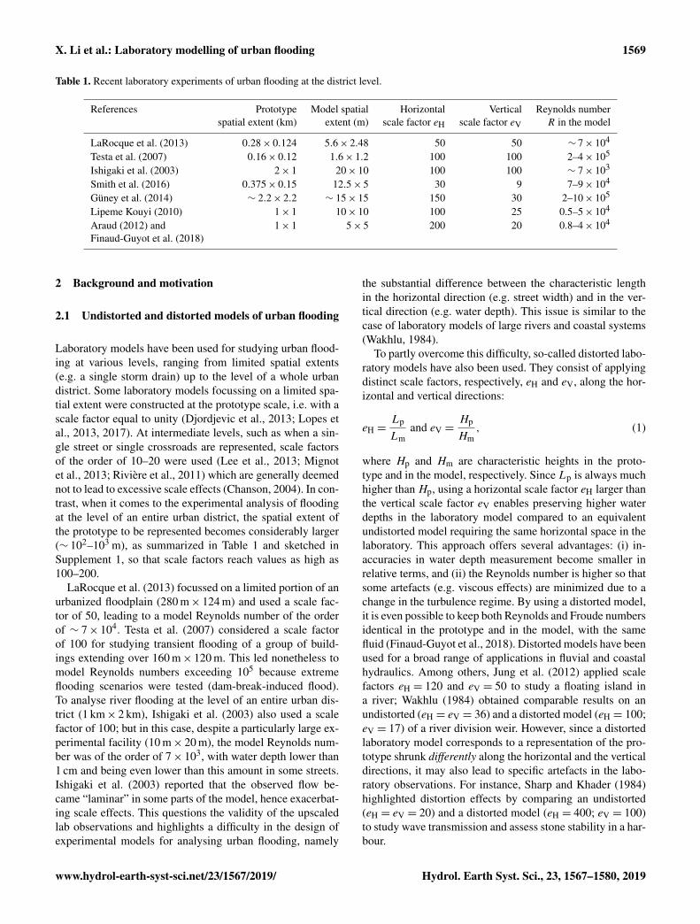
Figure 1. Recent laboratory models of urban flooding at the district level as a function of the horizontal and vertical scale factors, eH andeV. The grey shading qualitatively reveals the possible magnitude of (a) scale effects and (b) distortion effects; a range of maximum scalefactors (purple lines) and distortion ratio (orange lines) were recommended by Chanson (2004).

2.2 Recent studies based on distorted models of urbanflooding and potential artefacts

Figure 1 shows the horizontal and vertical scale factors usedin recent laboratory studies of urban flooding at the districtlevel. The grey shading in Fig. 1a suggests conceptually thatthe larger the scale factors, the greater the expected scale ef-fects, while Fig. 1b indicates that using a strongly distortedmodel (i.e. a large ratio eH/eV) also leads to specific arte-facts, which we refer to hereafter as distortion effects. Basedon experience, Chanson (2004) suggests keeping the ratioeH/eV below 5–10 (orange dotted lines in Fig. 1b).

An outdoor distorted model was used by Smith etal. (2016) to represent pluvial flooding in an urban districtof relatively limited extent (Table 1). The scale factors wereas low as eH = 30 and eV = 9 (distortion ratio: eH/eV = 3.3),thus minimizing potential scale effects. Similarly, Güney etal. (2014) used an outdoor distorted model of a large ur-ban district (Table 1), with eH = 150 and eV = 30 (distor-tion ratio: eH/eV = 5), to represent dam-break-induced floodwaves. The distortion ratio of these two models remains be-low the upper bound of 5–10, as recommended by Chan-son (2004). Lipeme Kouyi et al. (2010), Araud (2012) andFinaud-Guyot et al. (2018) considered the same geometricconfiguration (Supplement 1) involving seven streets alignedalong one direction, crossing seven other streets. The scalefactors used by Lipeme Kouyi et al. (2010) were eH = 100and eV = 25. The set-up of Araud (2012) and Finaud-Guyotet al. (2018) contains substantial improvements compared tothe initial set-up of Lipeme Kouyi et al. (2010), mainly re-garding the control of the inflow in each street separately,

but it uses a considerably higher horizontal scale factor(eH = 200) and, simultaneously, a smaller vertical scale fac-tor (eV = 20). This leads to a particularly high ratio eH/eV,equal to the upper limit of 10 suggested by Chanson (2004).If the model of Araud (2012) and Finaud-Guyot et al. (2018)had not been distorted, the Reynolds numbers would havebeen about 30 times lower (R ∼ 1×102

−1×103) than theyactually are (Table 1).

2.3 Specific objective of the present study

While the motivations for using a large distortion ratio be-tween the horizontal and vertical scale factors are not ar-guable (fit the model within a limited laboratory space, im-prove the accuracy of water depth measurement and maintaina sufficiently high Reynolds number), the assumption of hav-ing no artefacts in experimental observations performed ona strongly distorted model may legitimately be questioned.Among other aspects, the complex three-dimensional flowstructures observed in individual crossroads (Mignot et al.,2008, 2013; Rivière et al., 2011, 2014) suggest that “shrink-ing” the model vertically is likely to alter these flow struc-tures and hence also impair the representation of flow parti-tion in-between the streets. The influence of strong distortionin laboratory-scale models was investigated for some specificapplications, such as in coastal engineering (Ranieri, 2007;Sharp and Khader, 1984), but it has not been analysed to datein the context of laboratory models of urban flooding.

Therefore, in this paper, we aim to evaluate the artefactsarising from the use of distorted laboratory models in experi-mental studies of urban flooding at the district level. We base

Hydrol. Earth Syst. Sci., 23, 1567–1580, 2019 www.hydrol-earth-syst-sci.net/23/1567/2019/

X. Li et al.: Laboratory modelling of urban flooding 1571

our assessment on the reanalysis of two recent datasets, pre-sented, respectively, by Araud (2012) and by Velickovic etal. (2017). The latter does not represent a realistic urban dis-trict but solely a regular grid of obstacles, which is similarto a network of streets to some extent. We focus on the in-fluence of model distortion on the observed water depths anddischarge partition in-between the streets.

3 Data and methods

3.1 Datasets

Two datasets were reanalysed, corresponding, respectively,to an entire urban district and to a group of buildings. Theformer dataset was collected by Araud (2012) in the ICubelaboratory in Strasbourg (France) and was also presented byArrault et al. (2016) and Finaud-Guyot et al. (2018) (Fig. S3ain Supplement 2). The experimental model (5 m× 5 m) rep-resents an idealized urban district of 1 km× 1 km at the pro-totype scale. It contains a total of 14 streets of various widths(0.05–0.125 m) and 49 intersections (crossroads). The inflowdischarge was controlled in each street individually, the un-certainty of the inflow discharge is estimated at about 1 %(Fiaud-Guyot et al., 2018) and the outflow discharges weremonitored downstream of each street. The uncertainties inthe estimation of the outflow discharges are discussed inSect. 4.1. For several steady inflow discharges, the waterdepths along the centreline of streets were measured using anoptical gauge (1 mm accuracy; Figs. S4–S7). Hereafter, weconsider the experimental runs performed with a total inflowdischarge Qm of 20, 60, 80 and 100 m3 h−1 in the laboratorymodel (Table 2). In each test, 50 % of the total inflow dis-charge was fed to the west face of the model and 50 % to thenorth face of the model. The specific inflow discharge waskept the same for each street of a given face, the outflow dis-charge was estimated from a calibrated rating curve (Araud,2012). As detailed in Supplement 2–5, several measurementswere repeated, which allows appreciating the reproducibilityof the tests.

The second dataset was collected by Velickovic etal. (2017) in the Hydraulic Laboratory of UniversitéCatholique de Louvain, Belgium. A group of 5× 5 squareobstacles (buildings) of 0.30 m× 0.30 m were installed in ahorizontal flume 36 m× 3.6 m. Several layouts of obstacleswere considered, and we analyse three of them here (alignedwith the channel; Fig. S3b). For each of these layout, be-tween four and six experimental runs (Table 3) were con-ducted with various steady inflow discharges (accuracy offlowmeters: ∼ 1 L s−1). The three layouts differ by the dis-tance in-between the obstacles (i.e. the street widths) in thedirection normal to the main flow (0.0675, 0.10 and 0.135 m).Profiles of water depth (accuracy: 0.1 mm) were measuredwith movable ultrasonic probes along the centreline of thestreets aligned with the main flow direction. In contrast with

Figure 2. (a) Sketch of the initial interpretation of the laboratorymodel runs as various flooding scenarios represented with fixedscale factors. (b) Sketch of the interpretation in the present reanal-ysis, involving a single flood scenario represented with various ver-tical scale factors eV.

the dataset of Araud (2012), the flow partition in-between thestreets was not measured by Velickovic et al. (2017).

3.2 Method

As sketched in Fig. 2a, the initial interpretation of the var-ious experimental runs of Araud (2012) and Velickovic etal. (2017) was that each model run corresponds to a differentflooding scenario (i.e. a different total inflow discharge Qminto the urban district) represented with fixed scale factorseH and eV. In contrast, in the present reanalysis of the labo-ratory dataset, we propose considering that a single floodingscenario was represented in each laboratory model but thatthe various experimental runs actually correspond to differ-ent vertical scale factors eV. This new perspective is sketchedin Fig. 2b.

As detailed hereafter, we followed a three-step procedurefor the reanalysis. For each model, the procedure was as fol-lows:

1. Select one experimental run and assign to it plausiblescale factors eH and eV.

2. Estimate the scale factor eV corresponding to each ofthe other experimental runs, assuming that eH remainsunchanged and that all experimental runs simulate thesame flood scenario.

3. Upscale the experimental observations of each run tothe prototype scale and compare them to each other.

Step 1

We considered that Run 1 (Table 2) of Araud (2012) cor-responds to a representation of a given flooding scenario in

www.hydrol-earth-syst-sci.net/23/1567/2019/ Hydrol. Earth Syst. Sci., 23, 1567–1580, 2019

1572 X. Li et al.: Laboratory modelling of urban flooding

Table 2. Initial interpretation of the laboratory model runs as various flooding scenarios represented with fixed scale factors (Araud, 2012;Finaud-Guyot et al., 2018) vs. interpretation in the present reanalysis, involving a single flood scenario represented with various vertical scalefactors. Notations Qm and Qp refer to the total inflow in the laboratory model and in the prototype urban district, respectively.

Runs Qm Initial interpretation by Araud Interpretation in the present reanalysis: fixed(m3 h−1) (2012): fixed scale factors flood scenario, but varying vertical scale factor

Qp eH eV Qp eH eV d = eH/eV(m3 s−1) (–) (–) (m3 s−1) (–) (–) (–)

Run 1 100 497 200 20 497 200 20 10Run 2 80 398 23 8.6Run 3 60 298 28 7.1Run 4 20 99 58 3.4

Table 3. Interpretation of the dataset of Velickovic et al. (2017) in the present reanalysis. Notations Qm and Qp refer to the total inflowdischarge in the laboratory model and in the prototype, respectively.

Layouts Runs Qm Qp eH eV d = eH/eV(L s−1) (m3 s−1) (–) (–) (–)

Narrow streets Run 1 25 483 100 33.4 3along the main flow Run 2 35 26.7 3.7direction (width: 0.0675 m) Run 3 41 24.0 4.2

Run 4 50 21.0 4.8

Intermediate streets Run 1 43 483 100 23.3 4.3along the main Run 2 58 19.1 5.2flow direction (width: 0.10 m) Run 3 63 18.0 5.5

Run 4 75 16.1 6.2Run 5 86 14.7 6.8Run 6 103 13.0 7.7

Wide streets Run 1 52 483 100 20.5 4.9along the main flow Run 2 64 17.9 5.6direction (width: 0.135 m) Run 3 75 16.1 6.2

Run 4 80 15.4 6.5Run 5 92 14.0 7.1Run 6 99 13.3 7.5

a strongly distorted scale model, consistent with the orig-inal values eH = 200 and eV = 20 reported by Arrault etal. (2016).

Similarly, for the dataset of Velickovic et al. (2017), weconsidered that the street width (0.10 m), in the model layoutcharacterized by an intermediate street width, corresponds to10 m in the prototype. This sets the horizontal scale factor toeH = 100. Keeping eH = 100 for the two other layouts leadsto reproducing prototype street widths of 6.75 m for the nar-row street layout and 13.5 m for the wide street layout. Asshown in Table 3, we also assumed that the experimentallyobserved water depth (∼ 0.3 m) for the highest inflow dis-charge Qm in the layout with an intermediate street width(Run 6) corresponds to about 4 m in the prototype (i.e. ex-treme flooding conditions such as induced by a dam break).This leads to a vertical scale factor eV = 13 for this run (Ta-ble 3).

Step 2

For the dataset of Araud (2012), Runs 2–4 in Table 2 are nowassumed to represent the same flooding scenario as Run 1,with the same horizontal scale factor eH but with adjustedvertical scale factors eV. Similarly, all runs in Table 3 (datasetof Velickovic et al., 2017) represent the same flooding sce-nario as Run 6 of the intermediate street layout, but with dif-ferent vertical scale factors. For both datasets, the adjustedvalues of eV were derived as follows:

– The run selected in Step 1 was upscaled to the proto-type scale, enabling the determination of the inflow dis-charge Qp in the prototype.

– Knowing the inflow discharge Qm for each of the othermodel runs, the adjusted vertical scale factor was calcu-lated as eV = (Qp/Qm/eH)

2/3, consistent with Froudesimilarity.

Hydrol. Earth Syst. Sci., 23, 1567–1580, 2019 www.hydrol-earth-syst-sci.net/23/1567/2019/

X. Li et al.: Laboratory modelling of urban flooding 1573

The values of eV derived from this procedure are detailed inTables 2 and 3 for the two datasets. The model distortion,expressed as the ratio d between eH and eV, varies from 3 to7.7 in the dataset of Velickovic et al. (2017) and from 3.4 to10 in the dataset of Araud (2012).

Step 3

Finally, for each model, the experimental observations of allmodel runs (measured water depths and outflow discharges)were upscaled to the prototype scale and compared. This ap-proach is similar to the “scale series” method described byHeller (2011) and used by Erpicum et al. (2016), althoughhere we vary only the vertical scale factor.

If there were no artefacts arising from the model distor-tion, the prototype scale predictions from the different exper-imental runs should superimpose. In the following, we assessthe magnitude of the distortion effects by comparing the up-scaled observations from each experimental run with one se-lected reference, namely the experimental run correspondingto the weakest distortion (minimum value of d), for which wehave the highest confidence in prototype event replication:Run 4 (d = 3.4) in the dataset of Araud (2012) and Run 1 ofeach layout (d = 3, 4.3, 4.9) in the dataset of Velickovic etal. (2017).

4 Results

We first present an estimation of the experimental uncertain-ties (Sect. 4.1); then, we detail the effect of model distortionon the upscaled water depths (Sect. 4.2). Finally, we presentthe effect of model distortion on the partition of outflow dis-charges (Sect. 4.3).

4.1 Experimental uncertainties

The measurement accuracy and the fluctuations of water sur-face are considered the two main sources of uncertainty inthe experimental records of water depths. For the dataset ofAraud (2012), the accuracy of the optical gauge is about1 mm. As shown in Supplement 2, the water depths weremeasured twice at some locations for Run 3 (60 m3 h−1) andRun 2 (80 m3 h−1). The repeatability of the tests is evalu-ated by comparing the repeated measurements. As detailedin Supplement 3, the difference in water depths between twomeasurements remains below 2 mm for 90 % of the dataset.Therefore, we estimate here the water depth measurementuncertainty at about 2 mm. Representative profiles of mea-sured water depths (including repetitions) are displayed inSupplement 4, and they confirm the validity of this uncer-tainty estimate. Uncertainties arising from inaccuracies in theinflow discharge measurement are also lumped into this un-certainty estimate.

The discharge at the outlet of each street was estimatedfrom a rating curve corresponding to a weir at the down-

Figure 3. Upscaled water depth profiles in prototype in street 4of Araud (2012) predictions, colour shade represents the upscaledmeasurement uncertainty.

stream end of dedicated measurement channels (locateddownstream of each street outlet). The water depth measure-ments were performed at least three times for each modelrun. As detailed in Supplement 5, comparing the repeatedmeasurements demonstrates an excellent repeatability of theoutflow discharge estimates (Figs. S12–S15). Hence, themain source of uncertainty in the outflow discharge estimatesis assumed to stem from the accuracy of water depth mea-surement (1 mm) over the measurement weirs (Araud, 2012).This leads to about 2 %–6 % uncertainty in the outflow dis-charges, as shown in Fig. S16.

For the second dataset, the accuracy of the probes, as de-scribed by Velickovic et al. (2017), is 0.1 mm. Velickovic etal. (2017) also reported the standard deviation of the recordedwater depths at each probe location. We used this as a proxyfor estimating the flow variability. Figure S9 in Supplement 3shows the cumulative distribution function of this standarddeviation over all measured data in the three layouts and foreach experimental run. For 90 % of the measurement points,the standard deviation remains below 2–6 mm (depending onthe experimental run), which reflects considerable fluctua-tions in the free surface, particularly for the higher flow rates.

4.2 Effect of model distortion on predicted waterdepths

4.2.1 Dataset of Araud (2012)

All measured water depths were upscaled to the prototypescale using the vertical scale factors defined in Table 2. Asexemplified in Fig. 3 for street 4 (and in Figs. S17 and S18 inSupplement 6 for streets A, B, and C), the tests conductedwith the strongest distortion (d = 8.6 and d = 10) lead tothe lowest estimates of water depths at the prototype scale.Conversely, the highest predicted water depths correspond

www.hydrol-earth-syst-sci.net/23/1567/2019/ Hydrol. Earth Syst. Sci., 23, 1567–1580, 2019

1574 X. Li et al.: Laboratory modelling of urban flooding

Figure 4. Spatial distributions (a, c, e) and scatter plots (b, d, f) of the differences between the upscaled water depths in Run 3 (d = 7.1),2 (d = 8.6) and 1 (d = 10), and those derived from Run 4 (d = 3.4) from Araud (2012). The dashed purple lines indicate the range containing90 % of the data.

systematically to the upscaled measurements from the testsinvolving a weaker distortion (d = 3.4), except nearby thedownstream boundary conditions where all predicted wa-ter depths are close to each other. The tests conducted withd = 7.1 lead to intermediate estimates of water depths at theprototype scale. The reasons for these differences are dis-cussed in Sect. 5.1. Here, the uncertainty associated to theupscaled water depths is larger when the model distortion is

limited, since the absolute value of the measurement uncer-tainty remains the same in all model runs, but a larger verticalscale factor is applied.

In Figs. 4 and 5 and Table 4, we quantitatively compare theupscaled water depths obtained from the four different modelruns listed in Table 2. The model run with the weakest dis-tortion is used as a reference for comparisons. The followingobservations can be made:

Hydrol. Earth Syst. Sci., 23, 1567–1580, 2019 www.hydrol-earth-syst-sci.net/23/1567/2019/

X. Li et al.: Laboratory modelling of urban flooding 1575

Table 4. Differences between upscaled water depths derived from various runs of Araud (2012).

Indicators Run 3 (d = 7.1) Run 2 (d = 8.6) Run 1 (d = 10)vs. Run 4 (d = 3.4) vs. Run 4 (d = 3.4) vs. Run 4 (d = 3.4)

MD∗ (m) −0.058 −0.088 −0.10795th percentile (m) 0.077 0.075 0.0605th percentile (m) −0.181 −0.237 −0.247

∗ MD stands for mean difference.

Figure 5. Cumulative distribution function (CDF) of the differ-ences between upscaled water depths from the various model runsof Araud (2012); the grey lines represent the upscaled measurementuncertainties with various eV (the larger the eV, the deeper the linecolour).

– The scatter plots in Fig. 4 confirm that the water depthsderived from the model with the lowest distortion aregenerally higher than those derived from the othermodel runs.

– The dashed purple lines (and corresponding labels;Fig. 4b, d, f) indicate the range containing 90 % of thedata. This shows that, despite the uncertainties in themeasurements, the differences between the model runsincrease very consistently as the model distortion in-creases. This consistent trend is also emphasized by theevolution of the mean difference (MD in Table 4) from−0.058 to −0.107 as d varies from 7.1 to 10 as wellas by the cumulative distribution of the differences inupscaled water depths derived from the various modelruns (Fig. 5).

– The 5th percentile of the differences between the mod-els with varying distortions is of the order of −20 to−25 cm (Table 4). When compared to the order of mag-nitude of the absolute value of water depths (∼ 2 m), theeffect of model distortion in the tested configurations isof the order of 10 % of the upscaled water depths.

– The spatial distributions provided in Fig. 4 also revealthat the influence of model distortion tends to increasein the upstream part of the urban district (i.e. closer tothe north and west faces). Two reasons contribute to ex-plain this: (i) the water depths in the downstream partare mainly controlled by the free outflow boundariesand remain therefore more similar whatever the distor-tion; and (ii) the cumulated effect of friction (expectedto be underestimated in the more distorted models com-pared to the less distorted or undistorted models, as de-tailed in Sect. 5.1) is stronger in the upstream part of theflow.

4.2.2 Dataset of Velickovic et al. (2017)

Figure S19 in Supplement 7 displays the upscaled waterdepth profiles based on the dataset of Velickovic et al. (2017)and the scale factors defined in Table 3 for each of the threelayouts. The upscaled water depths in the three model layoutsdiffer substantially as the same discharge Qp is imposed (hpin narrow street: ∼ 5 m; median street: ∼ 3.5 m; wide street:∼ 2.5 m). Now, for each model layout separately, we com-pare the observations corresponding to various inflow dis-charges in the same way as in the dataset of Araud (2012). Itis found that the upscaled water depths in the urban area be-come systematically lower as the model distortion increases.This is observed consistently for the three layouts of obsta-cles (narrow, intermediate and wide streets), and the differ-ences arising from the change in model distortion greatly ex-ceed the estimated experimental uncertainty. This result isalso confirmed by the values of mean differences (MDs) re-ported in Table 5 as well as by the cumulative distributionfunctions of the differences in water depths (Fig. S20 in Sup-plement 7). In each layout, the model characterized by thelowest value of d was taken as a reference for comparison.

4.3 Effect of model distortion on outflow discharges

For the dataset of Araud (2012), the upscaled values of thedischarge at the outlet of each street are shown in Supple-ment 8 (Fig. S21). Although the differences in the outflowdischarge appear to be of the same order of magnitude as theexperimental uncertainties, the variation in the outflow dis-charge partition with d shows a consistent monotonous trend

www.hydrol-earth-syst-sci.net/23/1567/2019/ Hydrol. Earth Syst. Sci., 23, 1567–1580, 2019

1576 X. Li et al.: Laboratory modelling of urban flooding

Table 5. Differences between upscaled water depths derived from various runs of Velickovic et al. (2017).

Layouts Runs MD 95 % 5 %(m) percentile (m) percentile (m)

Narrow street d = 3.7 vs. d = 3 −0.27 −0.17 −0.36d = 4.2 vs. d = 3 −0.32 −0.22 −0.45d = 4.8 vs. d = 3 −0.52 −0.50 −0.66

Intermediate street d = 5.2 vs. d = 4.3 −0.24 −0.07 −0.40d = 5.5 vs. d = 4.3 −0.37 −0.21 −0.71d = 6.2 vs. d = 4.3 −0.47 −0.24 −0.62d = 6.8 vs. d = 4.3 −0.46 −0.38 −0.83d = 7.7 vs. d = 4.3 −0.77 −0.43 −1.19

Wide street d = 5.6 vs. d = 4.9 −0.45 −0.30 −0.79d = 6.2 vs. d = 4.9 −0.59 −0.44 −0.92d = 6.5 vs. d = 4.9 −0.63 −0.52 −0.97d = 7.1 vs. d = 4.9 −0.72 −0.55 −1.25d = 7.5 vs. d = 4.9 −0.75 −0.57 −1.25

∗ MD stands for mean difference.

Figure 6. (a) Upscaled outflow discharge in each street compared to the corresponding value deduced from the observations in the lessdistorted model (d = 3.4), and (b) ratio of the associated water depths from Araud (2012) and Finaud-Guyot et al. (2018). Red dashed linesrepresent the ±10 % range.

(increasing, constant or decreasing) in all outlet streets. Sincethe mass balance remains unchanged at the level of the wholedistrict, the direction of change in the outlet discharge variesfrom one street to the other. In Fig. 6a, we compare the up-scaled outflow discharge in each street to the correspondingvalue derived from the less distorted model (d = 3.4). Thechanges in the estimated outflow discharge when d is variedare in the range of ±10 % in 11 streets out of 14 (and are inthe range of ±12 % in 13 streets out of 14, with a maximumchange of +18 % in just a single street).

The magnitude of model distortion effects may differ fromone flow variable to the other (Heller, 2011). To be able to ap-preciate the relative influence of model distortion on the out-

flow discharge and on the water depths, for each street outlet(noted i), we estimated the change in upscaled water depth(hi/href) “associated” with the observed change in the out-flow discharge (Qi/Qref) when the model distortion is var-ied (from dref to di). To do so, using Froude similarity leadsto hi/href = (Qi/Qref)

2/3eV,i/eV,ref. As shown in Fig. 6, theresults indicate that, in the present case, the magnitude ofmodel distortion effects appears to be relatively comparablefor the water depths and the outflow discharges (of the orderof ±10 %).

Hydrol. Earth Syst. Sci., 23, 1567–1580, 2019 www.hydrol-earth-syst-sci.net/23/1567/2019/

X. Li et al.: Laboratory modelling of urban flooding 1577

5 Discussion

5.1 Relative importance of the main causes ofdistortion effects

The differences in the upscaled water depths as a functionof the model distortion d may result from differences in lo-calized flow features (e.g. local head losses at street inter-sections) and from more distributed effects, which in thepresent case are likely to dominate only along the mainlyone-dimensional flow regions (typically within a street). Thelatter effects may be categorized into three types:

– differences in the relative importance of the bottomroughness,

– differences in the relative importance of viscosity ef-fects,

– differences in the aspect ratio (ratio between waterdepth and street width) of the flow section, notably af-fecting the secondary currents and velocity profiles ofstreamline velocity.

It is possible that the third of these effects has a substantial in-fluence on the flow. However, the available datasets, involv-ing only observed water depths and discharges at the modeloutlets, do not enable investigating these more localized ef-fects in detail. This could be achieved by means of new ex-periments with detailed velocity measurements within the ur-ban district. 2-D and 3-D computational modelling may alsobe useful in this respect, the former enabling us to accountfor the spatial variations of flow characteristics and the lattergiving us full access to the complex flow fields developing atthe street intersections.

Nonetheless, we appreciate here the influence of the firsttwo types of effects, which are of relevance to mainly one-dimensional flow regions. To do so, we estimate the energyslope Sf,p at the prototype scale in the various model config-urations based on the Darcy–Weisbach equation.

(2)

In this equation, the friction coefficient fm can be computedas a function of the Reynolds number Rm and the relativeroughness height ks,m/RH,m using the explicit approximationof the Colebrook–White formula given by Yen (2002). Theroughness height ks,m was taken to be equal to 10−5 m torepresent the smooth bottom and walls of the experimentalset-ups.

Figure S22 shows the values of parameters Rm,ks,m/RH,m, fm, hm/RH,m, and F , which are representativeof the flow conditions at the street inlets in the various ex-perimental runs of Araud (2012). Given the values of Rmand ks,m/RH,m, the flow is in a transitional regime in theMoody diagram. All these parameters change substantiallywhen the model distortion d is varied (Fig. S23). As d isincreased, the friction coefficient fm decreases systemati-cally (fi,m/fref,m ∼ 0.8) due to the joint effect of a higherReynolds number and a lower relative roughness height(ks,m/RH,m). Similarly, the Froude number tends to slightlyincrease with the model distortion. In contrast, parameterhm/RH,m shows a considerable systematic increase (1.6–2.3)as d increases due to the change in the aspect ratio of the flowsection. The resulting energy slope Sf,m in the inlet streets ineach model run and the corresponding upscaled values Sf,pare presented in Fig. 7. The energy slope is lower in majorstreets (4, C, F) and in the straight streets (A, B). The en-ergy slope Sf,m in the model increases monotonously with themodel distortion (mainly due to the increased wetted perime-ter), whereas the energy slope Sf,p at the prototype scale de-clines as d is increased (Fig. 7b). This results from a “com-petition” between the increase in Sf,m and a decrease in theratio eV/eH, as d increases. This effect appears dominant inthe mainly one-dimensional flow regions.

5.2 Reference used for comparison

Here, we used the “less distorted” models as a reference forour comparisons since the aim is to assess the influence ofmodel distortion. However, given that we simply reanalysedalready existing datasets obtained in experiments which werenot designed for the sake of investigating the effect of modeldistortion in the first place, these less distorted models arealso those characterized by the largest vertical scale factors,hence enhancing other artefacts such as stronger viscosity ef-fects (see asterisks in Fig. 1). Also, the upscaled measure-ment uncertainties are at a maximum in this case, as can beseen in Fig. 3. Therefore, the present study needs to be com-plemented by new tailored experiments involving a modelseries (Heller, 2011) with various levels of distortion and in-cluding a valid reference model, i.e. at least one model with-out distortion and that is characterized by sufficiently smallscale factors so that viscosity effects and experimental un-certainties are kept to a minimum. This may be achieved byconsidering a model series in which the vertical scale factoreV is kept constant in all models, while only the horizontalscale factor eH is varied. This approach contrasts with theprocedure followed here in which eH was constant and eVwas varied to take benefit of existing datasets.

www.hydrol-earth-syst-sci.net/23/1567/2019/ Hydrol. Earth Syst. Sci., 23, 1567–1580, 2019

1578 X. Li et al.: Laboratory modelling of urban flooding

Figure 7. Distortion effect on energy slope of (a) scale models and (b) the model in prototype (dataset of Araud, 2012).

6 Conclusions

Laboratory-scale models representing flooding of an entireurban district are usually distorted, in the sense that the ver-tical scale factor (Hp/Hm) is often considerably smaller thanthe horizontal one. This paper evaluates the influence ofthe model distortion on the upscaled values of water depthsand outflow discharge for relatively extreme flood conditions(water depth and flow velocity of the order of 1–2 m and 0.5–2 m s−1 at the prototype scale). Two existing experimentaldatasets were reanalysed for this purpose. The results showthat the stronger the model distortion, the lower the valuesof the upscaled water depths, whereas the influence on flowpartition at the outlet of the street appears more complex.

The change in the upscaled water depths was found to beof the order of 10 % when the distortion of the model wasvaried by a factor of 3. Moreover, a deviation of about 10 %was also obtained for the outflow discharges. This is of thesame order as the influence of small-scale obstacles, as re-ported by Bazin et al. (2017).

For the water depths, the effect of varying the model dis-tortion was found to be generally larger than the measure-ment uncertainties, whereas both effects are comparable forthe discharge at the street outlets in the tested configurations.Note that the relative measurement uncertainties are smallerin distorted models than in undistorted models.

The uncertainty in the upscaled water depths is consid-erably larger in the models with limited distortion, becausethey also correspond to the highest vertical scale factors. Us-ing those results as a reference seems sensible for assessingthe effect of distortion since they correspond to the lowestvalues of d , but at the same time it is somehow problematicto use the results with the highest uncertainty as a reference(e.g. Figs. S17–S18). To overcome this issue, future experi-

mental research should involve “model series” in which thehorizontal scale factor eH is reduced without changing thevertical scale factor eV. This will enable the reduction of theinfluence of distortion without increasing the error in the es-timated water depths, but this requires the collection of newexperimental measurements which are presently lacking.

This study is a contribution towards a deeper understand-ing of small-scale flow processes which govern urban flood-ing and need to be incorporated in urban hydrological mod-els, either explicitly or through parametrization. In future,more controlling parameters should also be considered, suchas the bottom slope, and computational modelling shouldcomplement the laboratory experiments (e.g. Ichiba et al.,2018; Ozdemir et al., 2013). Moreover, in real-world urbanflooding, the urban drainage system may also have a sub-stantial influence. Laboratory modelling of dual drainage be-comes even more intricate due to the combination of pressur-ized and surface flow (e.g. Rubinato et al., 2017). This posesadditional constraints on the design of the scale models andleads to extra experimental challenges which deserve furtherresearch. Finally, existing experiments of urban flooding atthe district level have delivered mostly discharge and waterdepth data, but there is a need for more pointwise velocitymeasurements (e.g. Martins et al., 2018) to gain deeper in-sights into the flow processes.

Data availability. The data presented in this paper can be accessedfrom the dataset listed in the references (Li et al., 2019).

Supplement. The supplement related to this article is availableonline at: https://doi.org/10.5194/hess-23-1567-2019-supplement.

Hydrol. Earth Syst. Sci., 23, 1567–1580, 2019 www.hydrol-earth-syst-sci.net/23/1567/2019/

X. Li et al.: Laboratory modelling of urban flooding 1579

Author contributions. XL conducted the analysis and wrote the firstversion of the paper, which was revised by BD. PA and BD formu-lated the research question. PFG shared the ICube experimental dataand, together with MB, helped with the analysis and interpretationof the dataset. BD, EM, SE, PA and MP supported the analysis andinterpretation of the results. All co-authors revised successive ver-sions of the paper.

Competing interests. The authors declare that they have no conflictof interest.

Acknowledgements. This research was partly funded through agrant for Concerted Research Actions (grant no. ARC 13-17/01)financed by the Wallonia-Brussels Federation, and it also benefittedfrom the support of French Community of Belgium with the fi-nancing of FRIA grant. The authors gratefully acknowledge SandraSoares-Frazão (Université Catholique de Louvain, Belgium) forsharing the experimental datasets.

Edited by: Marie-Claire ten VeldhuisReviewed by: two anonymous referees

References

Araud, Q.: Simulation des écoulements en milieu urbain lors d’unévénement pluvieux extrême, Université de Strasbourg, 2012.

Arrault, A., Finaud-Guyot, P., Archambeau, P., Bruwier, M.,Erpicum, S., Pirotton, M., and Dewals, B.: Hydrodynam-ics of long-duration urban floods: experiments and numeri-cal modelling, Nat. Hazards Earth Syst. Sci., 16, 1413–1429,https://doi.org/10.5194/nhess-16-1413-2016, 2016.

Bazin, P.-H., Mignot, E., and Paquier, A.: Comput-ing flooding of crossroads with obstacles using a 2-D numerical model, J. Hydraul. Res., 55, 72–84,https://doi.org/10.1080/00221686.2016.1217947, 2017.

Brown, R. and Chanson, H.: Suspended sediment properties andsuspended sediment flux estimates in an inundated urban en-vironment during a major flood event, Water Resour. Res., 48,W11523, doi:10.1029/2012WR012381, 2012.

Brown, R. and Chanson, H.: Turbulence and suspended sedimentmeasurements in an urban environment during the BrisbaneRiver flood of january 2011, J. Hydraul. Eng., 139, 244–253,https://doi.org/10.1061/(ASCE)HY.1943-7900.0000666, 2013.

Chanson, H.: 14 – Physical modelling of hydraulics, in: Hydraulicsof Open Channel Flow (Second Edition), edited by: Chanson, H.,253–274, Butterworth-Heinemann, Oxford, 2004.

Chen, Y., Zhou, H., Zhang, H., Du, G., and Zhou, J.: Urban floodrisk warning under rapid urbanization, Environ. Res., 139, 3–10,https://doi.org/10.1016/j.envres.2015.02.028, 2015.

Djordjevic, S., Saul, A. J., Tabor, G. R., Blanksby, J., Galam-bos, I., Sabtu, N., and Sailor, G.: Experimental and numer-ical investigation of interactions between above and belowground drainage systems, Water Sci. Technol., 67, 535–542,https://doi.org/10.2166/wst.2012.570, 2013.

Dottori, F., Di Baldassarre, G., and Todini, E.: Detailed data iswelcome, but with a pinch of salt: Accuracy, precision, and un-

certainty in flood inundation modeling, Water Resour. Res., 49,6079–6085, 2013.

Dottori, F., Figueiredo, R., Martina, M. L. V., Molinari, D.,and Scorzini, A. R.: INSYDE: a synthetic, probabilistic flooddamage model based on explicit cost analysis, Nat. HazardsEarth Syst. Sci., 16, 2577–2591, https://doi.org/10.5194/nhess-16-2577-2016, 2016.

Erpicum, S., Tullis, B. P., Lodomez, M., Archambeau, P., De-wals, B. J., and Pirotton, M.: Scale effects in physicalpiano key weirs models, J. Hydraul. Res., 54, 692–698,https://doi.org/10.1080/00221686.2016.1211562, 2016.

Finaud-Guyot, P., Garambois, P.-A., Araud, Q., Lawniczak, F.,François, P., Vazquez, J., and Mosé, R.: Experimental insight forflood flow repartition in urban areas, Urban Water J., 15, 242–250, https://doi.org/10.1080/1573062X.2018.1433861, 2018.

Gaines, J. M.: Flooding: Water potential, Nature, 531, 54–55, 2016.Güney, M. S., Tayfur, G., Bombar, G., and Elci, S.: Dis-

torted Physical Model to Study Sudden Partial Dam BreakFlows in an Urban Area, J. Hydraul. Eng., 140, 05014006,https://doi.org/10.1061/(ASCE)HY.1943-7900.0000926, 2014.

Heller, V.: Scale effects in physical hydraulic engi-neering models, J. Hydraul. Res., 49, 293–306,https://doi.org/10.1080/00221686.2011.578914, 2011.

Heller, V., Hager, W. H., and Minor, H.-E.: Scale effects in subaeriallandslide generated impulse waves, Exp. Fluids, 44, 691–703,https://doi.org/10.1007/s00348-007-0427-7, 2008.

Hettiarachchi, S., Wasko, C., and Sharma, A.: Increase in flood riskresulting from climate change in a developed urban watershed –the role of storm temporal patterns, Hydrol. Earth Syst. Sci., 22,2041–2056, https://doi.org/10.5194/hess-22-2041-2018, 2018.

Ichiba, A., Gires, A., Tchiguirinskaia, I., Schertzer, D., Bompard,P., and Ten Veldhuis, M.-C.: Scale effect challenges in urban hy-drology highlighted with a distributed hydrological model, Hy-drol. Earth Syst. Sci., 22, 331–350, https://doi.org/10.5194/hess-22-331-2018, 2018.

Ishigaki, T., Keiichi, T., and Kazuya, I.: Hydraulic model tests ofinundation in urban area with underground space, Theme B,Proc. of XXX IAHR Cogress, Greece, available from: https://ci.nii.ac.jp/naid/10029665177/en/, 487–493, 2003.

Jung, S., Kang, J., Hong, I., and Yeo, H.: Case study: Hy-draulic model experiment to analyze the hydraulic fea-tures for installing floating islands, Sci. Res., 4, 90–99,https://doi.org/10.4236/eng.2012.42012, 2012.

Kreibich, H., Van Den Bergh, J. C. J. M., Bouwer, L. M., Bubeck,P., Ciavola, P., Green, C., Hallegatte, S., Logar, I., Meyer, V.,Schwarze, R., and Thieken, A. H.: Costing natural hazards, Nat.Clim. Change, 4, 303–306, 2014.

LaRocque, L. A., Elkholy, M., Chaudhry, M. H., andImran, J.: Experiments on Urban Flooding Causedby a Levee Breach, J. Hydraul. Eng., 139, 960–973,https://doi.org/10.1061/(ASCE)HY.1943-7900.0000754, 2013.

Lee, S., Nakagama, H., Kawaike, K., and Zhang, H.: Experimentalvalidation pf interaction model at storm drain for development ofintergrated urbain inundation model, J. Jpn. Soc. Lubr. Eng., 69,109–114, https://doi.org/10.2208/jscejhe.69.I_109, 2013.

Lehmann, J., Coumou, D., and Frieler, K.: Increased record-breaking precipitation events under global warming, Clim.Change, 132, 501–515, https://doi.org/10.1007/s10584-015-1434-y, 2015.

www.hydrol-earth-syst-sci.net/23/1567/2019/ Hydrol. Earth Syst. Sci., 23, 1567–1580, 2019

1580 X. Li et al.: Laboratory modelling of urban flooding

Li, X., Erpicum, S., Bruwier, M., Mignot, E., Finaud-Guyot,P., Archambeau, P., Pirotton, M., and Dewals, B.: Sup-porting data for: “Laboratory modelling of urban flooding:strengths and challenges of distorted scale models” (Data set),https://doi.org/10.5281/zenodo.2586900, 2019.

Lipeme Kouyi, G., Rivière, N., Vidalat, V., Becquet, A., Chocat,B., and Guinot, V.: Urban flooding: One-dimensional modellingof the distribution of the discharges through cross-road inter-sections accounting for energy losses, Water Sci. Technol., 61,2021–2026, https://doi.org/10.2166/wst.2010.133, 2010.

Liu, D.: Water supply: China’s sponge cities to soak up rainwater,Nature, 537, 307, https://doi.org/10.1038/537307c, 2016.

Lopes, P., Leandro, J., Carvalho, R. F., Pascoa, P., and Mar-tins, R.: Numerical and experimental investigation of a gullyunder surcharge conditions, Urban Water J., 12, 468–476,https://doi.org/10.1080/1573062X.2013.831916, 2013.

Lopes, P., Carvalho, R. F., and Leandro, J.: Numerical and exper-imental study of the fundamental flow characteristics of a 3-Dgully box under drainage, Water Sci. Technol., 75, 2204–2215,https://doi.org/10.2166/wst.2017.071, 2017.

Mallakpour, I. and Villarini, G.: The changing nature of floodingacross the central United States, Nat. Clim. Change, 5, 250–254,https://doi.org/10.1038/nclimate2516, 2015.

Martins, R., Rubinato, M., Kesserwani, G., Leandro, J., Djord-jevic, S., and Shucksmith, J. D.: On the Characteristics ofVelocities Fields in the Vicinity of Manhole Inlet GratesDuring Flood Events, Water Resour. Res., 54, 6408–6422,https://doi.org/10.1029/2018WR022782, 2018.

Mignot, E., Paquier, A., and Rivière, N.: Experimental andnumerical modeling of symmetrical four-branch supercriti-cal cross junction flow, J. Hydraul. Res., 46, 723–738,https://doi.org/10.3826/jhr.2008.2961, 2008.

Mignot, E., Zeng, C., Dominguez, G., Li, C.-W., Rivière, N., andBazin, P.-H.: Impact of topographic obstacles on the dischargedistribution in open-channel bifurcations, J. Hydrol., 494, 10–19,https://doi.org/10.1016/j.jhydrol.2013.04.023, 2013.

Mignot, E., Li, X., and Dewals, B.: Experimental modellingof urban flooding: A review, J. Hydrol., 568, 334–342,https://doi.org/10.1016/j.jhydrol.2018.11.001, 2019.

Molinari, D. and Scorzini, A. R.: On the influence of input dataquality to Flood Damage Estimation: The performance of the IN-SYDE model, Water, 9, 688, https://doi.org/10.3390/w9090688,2017.

Moy de Vitry, M., Dicht, S., and Leitão, J. P.: floodX: ur-ban flash flood experiments monitored with conventionaland alternative sensors, Earth Syst. Sci. Data, 9, 657–666,https://doi.org/10.5194/essd-9-657-2017, 2017.

Novak, P.: Scaling Factors and Scale Effects in Modelling HydraulicStructures, in: Symposium on Scale Effects in Modelling Hy-draulic Structures, edited by: Kobus, H., International Associa-tion for Hydraulic Reasearch (IAHR), 0.3–1–0.3–5, 1984.

Ozdemir, H., Sampson, C. C., de Almeida, G. A. M., and Bates, P.D.: Evaluating scale and roughness effects in urban flood mod-elling using terrestrial LIDAR data, Hydrol. Earth Syst. Sci., 17,4015–4030, https://doi.org/10.5194/hess-17-4015-2013, 2013.

Park, H., Cox, D. T., Lynett, P. J., Wiebe, D. M., and Shin,S.: Tsunami inundation modeling in constructed environments:A physical and numerical comparison of free-surface eleva-

tion, velocity, and momentum flux, Coast. Eng., 79, 9–21,https://doi.org/10.1016/j.coastaleng.2013.04.002, 2013.

Ranieri, G.: The surf zone distortion of beach profiles insmalle-scale coastal models, J. Hydraul. Res., 45, 261–269,https://doi.org/10.1080/00221686.2007.9521761, 2007.

Rivière, N., Travin, G., and Perkins, R. J.: Subcritical open chan-nel flows in four branch intersections, Water Resour. Res., 47,W10517, https://doi.org/10.1029/2011WR010504, 2011.

Rivière, N., Travin, G., and Perkins, R. J.: Transcritical flows inthree and four branch open-channel intersections, J. Hydraul.Eng., 140, 04014003, https://doi.org/10.1061/(ASCE)HY.1943-7900.0000835, 2014.

Rubinato, M., Martins, R., Kesserwani, G., Leandro, J., Djordje-vic, S., and Shucksmith, J.: Experimental calibration and val-idation of sewer/surface flow exchange equations in steadyand unsteady flow conditions, J. Hydrol., 552, 421–432,https://doi.org/10.1016/j.jhydrol.2017.06.024, 2017.

Sharp, J. J. and Khader, M. H. A.: Scale effects in Harbour Mod-els Invovling Permeable Rubble Mound Structures, in: Sympo-sium on Scale Effects in Modelling Hydraulic Structures, editedby: Kobus, H., International Association for Hydraulic Reasearch(IAHR), 7.12-1–.12–5, 1984.

Smith, G. P., Rahman, P. F., and Wasko, C.: A comprehen-sive urban floodplain dataset for model benchmarking, Inter-national Journal of River Basin Management, 14, 345–356,https://doi.org/10.1080/15715124.2016.1193510, 2016.

Testa, G., Zuccala, D., Alcrudo, F., Mulet, J., and Soares-Frazão, S.: Flash flood flow experiment in a sim-plified urban district, J. Hydraul. Res., 45, 37–44,https://doi.org/10.1080/00221686.2007.9521831, 2007.

UNISDR: The human cost of weather related disasters, CRED1995–2015, United Nations, Geneva, 2015.

Velickovic, M., Zech, Y., and Soares-Frazão, S.: Steady-flow experiments in urban areas and anisotropicporosity model, J. Hydraul. Res., 55, 85–100,https://doi.org/10.1080/00221686.2016.1238013, 2017.

Wakhlu, O. N.: Scale Effects in Hydraulic Model Studies, in: Sym-posium on Scale Effects in Modelling Hydraulic Structures,edited by: Kobus, H., International Association for HydraulicReasearch (IAHR), 2.13-1–2.13-6, 1984.

Wright, N.: Advances in flood modelling helping toreduce flood risk, Proceedings of the Institutionof Civil Engineers: Civil Engineering, 167, 52–52,https://doi.org/10.1680/cien.2014.167.2.52, 2014.

Yen, B. C.: Open channel flow resistance, J. Hydraul. Eng., 128,20–39, 2002.

Zhou, Q., Leng, G., and Huang, M.: Impacts of future climatechange on urban flood volumes in Hohhot in northern China:benefits of climate change mitigation and adaptations, Hydrol.Earth Syst. Sci., 22, 305–316, https://doi.org/10.5194/hess-22-305-2018, 2018.

Zhou, Q., Yu, W., Chen, A. S., Jiang, C., and Fu, G.: ExperimentalAssessment of Building Blockage Effects in a Simplified UrbanDistrict, Procedia Engineer., 154, 844–852, 2016.

Hydrol. Earth Syst. Sci., 23, 1567–1580, 2019 www.hydrol-earth-syst-sci.net/23/1567/2019/