Atmos. Chem. Phys., 17, 6215–6225, 2017www.atmos-chem-phys.net/17/6215/2017/doi:10.5194/acp-17-6215-2017© Author(s) 2017. CC Attribution 3.0 License.

Technical note: Boundary layer height determination from lidarfor improving air pollution episode modeling: developmentof new algorithm and evaluationTing Yang1, Zifa Wang1, Wei Zhang2, Alex Gbaguidi1, Nobuo Sugimoto3, Xiquan Wang1, Ichiro Matsui3, andYele Sun1

1State Key Laboratory of Atmospheric Boundary Layer Physics and Atmospheric Chemistry, Institute ofAtmospheric Physics, Chinese Academy of Sciences, Beijing 100029, China2Aviation Meteorological Center of China, Beijing 100021, China3National Institute for Environmental Studies, 16-2 Onogawa, Tsukuba, 305-8506, Japan

Correspondence to: Ting Yang (tingyang@mail.iap.ac.cn) and Zifa Wang (zifawang@mail.iap.ac.cn)

Received: 12 November 2016 – Discussion started: 3 January 2017Revised: 7 April 2017 – Accepted: 14 April 2017 – Published: 22 May 2017

Abstract. Predicting air pollution events in the low atmo-sphere over megacities requires a thorough understanding ofthe tropospheric dynamics and chemical processes, involv-ing, notably, continuous and accurate determination of theboundary layer height (BLH). Through intensive observa-tions experimented over Beijing (China) and an exhaustiveevaluation of existing algorithms applied to the BLH deter-mination, persistent critical limitations are noticed, in par-ticular during polluted episodes. Basically, under weak ther-mal convection with high aerosol loading, none of the re-trieval algorithms is able to fully capture the diurnal cycleof the BLH due to insufficient vertical mixing of pollutantsin the boundary layer associated with the impact of gravitywaves on the tropospheric structure. Consequently, a new ap-proach based on gravity wave theory (the cubic root gradi-ent method: CRGM) is developed to overcome such weak-ness and accurately reproduce the fluctuations of the BLHunder various atmospheric pollution conditions. Comprehen-sive evaluation of CRGM highlights its high performance indetermining BLH from lidar. In comparison with the existingretrieval algorithms, CRGM potentially reduces related com-putational uncertainties and errors from BLH determination(strong increase of correlation coefficient from 0.44 to 0.91and significant decreases of the root mean square error from643 to 142 m). Such a newly developed technique is undoubt-edly expected to contribute to improving the accuracy of airquality modeling and forecasting systems.

1 Introduction

The boundary layer height (BLH) illustrates the relationshipsbetween air pollution intensity, duration, and scope; it con-stitutes an important factor influencing the diffusion of pol-lutants in the low atmosphere (Tie et al., 2007; Quan et al.,2013). An increase of air pollutants is often associated with ashallow BLH, while a decrease of pollutants is accompaniedby obvious uplift of the BLH. Besides the physical effects,BLH can also affect the precursor particles’ concentrationand distribution, which might affect the chemical transfor-mation of fine particulate matter (Ansari and Pandis, 1998).BLH is also a key parameter for air pollution models; it de-termines the volume available for the dispersion of pollutantsand is involved in many predictive and diagnostic methodsand/or models that assess pollutant concentrations (Seibertet al., 2000). The bias of the BLH between the air qualitymodel and observation is a potential cause of model’s dif-ficulties to accurately forecast air pollution episodes (Dab-berdt et al., 2004). Therefore, accurately acquiring the BLH,especially during polluted episodes, is of great significanceto investigating air pollution issues.

Many techniques have been developed to determine theBLH, for example, through radiosonde measurements (Stull,1988), remote sensing (Emeis et al., 2007), laboratory exper-iments (Park et al., 2001), and model simulations (Dandou etal., 2009). The high spatiotemporal resolutions make aerosollidar techniques (light detection and ranging) one of the most

Published by Copernicus Publications on behalf of the European Geosciences Union.

6216 T. Yang et al.: Boundary layer height determination from lidar

suitable systems for analyzing the boundary layer structureand determining the BLH (Flamant et al., 1997). Due tothe complex vertical structure of boundary layer, numerousmethods have been proposed to accurately retrieve the BLHfrom lidar, such as the maximum variance method (Hooperand Eloranta, 1986), fitting idealized profile method (Steyn etal., 1999), first point method (Boers and Melfi, 1987), thresh-old method (Dupont et al., 1994), wavelet transform method(Davis et al., 2000; Baars et al., 2008), first gradient method(Flamant et al., 1997), logarithm gradient method (Senff etal., 1996), and normalized gradient method (He et al., 2006).However, so far most of the algorithms have been tested andvalidated only over relatively unperturbed homogeneous ter-rain, for example, oceans (Melfi et al., 1985; Flamant et al.,1997), rural areas, and clean meteorological conditions (Pi-ironen and Eloranta, 1995). Limited evaluations of the algo-rithms have been carried out in polluted megacities in de-veloping countries, associated with a high density of build-ings and heavy anthropogenic pollutants. Nevertheless, thesurface roughness and high aerosol loading in the boundarylayer result in a more complex structure and increase the dif-ficulty of BLH retrieval based on these algorithms.

As one of the largest megacities in Asia affected by heavypollution, Beijing provides a particular challenge to resolv-ing the BLH determination. Specifically, the movement ofthe atmosphere can affect the distribution of pollutant con-centrations; moreover, vertically propagating gravity wavesinfluence the structure of the atmosphere and cause some ofthe spatiotemporal variability (Fritts and Alexander, 2003).Gravity waves thus provide new theoretical insights for thedevelopment of a new algorithm in determining BLH by tak-ing into account a probably insufficient vertical mixing ofpollutants under weak thermal convection and pollutant ac-cumulation at high altitudes due to long-range transport pro-cesses. Beijing, often governed by stagnant meteorologicalconditions, is surrounded by mountains to the west, north,and northeast, and characterized by favorable conditions togenerate and maintain gravity waves. Such specific atmo-spheric conditions provide the opportunity to obtain insightsinto the difficulties related to the BLH retrieval based on ex-isting algorithms and to evaluate the performance of a newapproach that considers the impact of gravity waves. Basedon an intensive observation campaign over Beijing, this pa-per aims at delving into the limitations of current retrievalalgorithms employed for BLH determination from lidar dur-ing a polluted period and at coming up with the develop-ment of a new algorithm compatible with all atmosphericpollution conditions. This work therefore provides, for thefirst time, a prototype of how to integrate into the BLH re-trieval process gravity waves and the resulting complexityof the low-troposphere structure under conditions of heavyaerosol loading. Section 2 presents a detailed description ofthe lidar observational experiment setting over Beijing anddiscusses the limitations of current algorithms for BLH re-trieval; Sect. 3 discusses the development of a new algo-

rithm; Sect. 4 presents the comprehensive evaluation of thenew retrieval algorithm and comparative analysis with exist-ing methods; and conclusion and environmental implicationsare given in Sect. 5.

2 Lidar experiment setting over Beijing and evaluationof existing BLH retrieval algorithms

2.1 Lidar observation campaign

Beijing, the capital of China, is located at 39◦56′ N,116◦20′ E on the northwest border of the great North ChinaPlain. It is surrounded by the Yan Mountains to the west,north, and northeast. The topography favors accumulationof pollutants. The air pollution is critically high, with thepeak concentration of PM2.5 exceeding 500 µg m−3 (Sunet al., 2014). An intensive observation campaign was con-ducted from 1 July to 16 September 2008 at the Insti-tute of Atmospheric Physics (IAP), Chinese Academy ofSciences (39◦58′28′′ N, 116◦22′16′′ E), located between thenorth third and fourth ring roads in Beijing and consideredas a highly polluted urban site. A dual-wavelength (1064,532 nm) depolarization lidar developed by the National In-stitute for Environmental Studies, Japan, sits on the rooftopof a 28 m high building. The lidar is used to retrieve the 6 mspace-resolved and 10 s time-resolved aerosol vertical struc-ture, but only for altitudes > 100 m due to an incomplete over-lap between the field of telescope view and the laser beam.More details of the lidar parameters can be found in the re-search of Sugimoto et al. (2002) and Yang et al. (2010).PM2.5 sampling was continuously conducted near the lidarsite. Potential temperature and relative humidity observed byradiosonde are integrated into the classic methods to retrievethe BLH and are employed to evaluate new algorithms (Stull,1988).

An unprecedented 78-day intensive radiosonde campaignwas conducted over the Institute of Atmospheric Physicssite (four times per day: 02:00, 08:00, 14:00, and 20:00 lo-cal standard time) in line with the lidar campaign at a ra-diosonde observatory located in southern Beijing (39◦48′ N,116◦28′ E). Daily PM2.5 concentrations observed over the In-stitute of Atmospheric Physics site between July and Septem-ber 2008 are shown in Fig. 1. A typical extended pol-luted episode occurred between 24 and 27 July, when thePM2.5 concentration exceeded the Grade III National Am-bient Air Quality Standards (moderate pollution, GB3095-2012, 115 µg m−3, 24 h average). The beginning and end ofthe pollution episode were on 24 and 28 July, respectively,while 27 July was the heaviest pollution day during the cam-paign, with a PM2.5 concentration of 195 µg m−3. On 27 July,the southeastern edge of a low-pressure system of northernChina prevailed over Beijing, inducing southerly flows. Un-der such meteorological conditions, accumulation of pollu-tants (due to long-range transport from neighboring regions)

Atmos. Chem. Phys., 17, 6215–6225, 2017 www.atmos-chem-phys.net/17/6215/2017/

T. Yang et al.: Boundary layer height determination from lidar 6217

Figure 1. Daily variation of the PM2.5 concentration between July and September 2008 at IAP. The dotted line represents the definition of amoderate pollution day (PM2.5 = 115 µg m−3), and 24, 27 and 28 July are highlighted.

occurs over the southern area (Chan and Yao, 2008). Below850 hPa, warm advection over northern China triggers a sig-nificant increase of air temperature at low altitudes, prevent-ing the vertical diffusion of pollutants (Fig. S1 in the Sup-plement). This presents a typical condition for evaluating theperformance of existing retrieval algorithms in determiningthe BLH.

2.2 Existing gradient algorithm for BLH determination

In normal conditions of an aerosol-laden boundary layer andclean overlying free atmosphere, the gradient of the range-squared-corrected signal (RSCS) exhibits a strong negativepeak at the transition between the boundary layer and free at-mosphere. Based on this principle, gradient algorithms wereproposed and had become the most widely used ones. In thispaper, we focus on the three most popular gradient meth-ods, including the first gradient method (GM), first loga-rithm gradient method (LGM), and first normalized gradi-ent method (NGM). The optical power measured by lidaris proportional to the signal backscattered of particles andmolecules present in the atmosphere. The lidar signal can beexpressed by Eq. (1) below:

RS(λ,r)=C

r2E0[βm(λ,r)+βp(λ,r)

]T 2(λ,r)+RS0, (1)

where βp(λ,r) and βm(λ,r) are the particular and molecularbackscatter coefficients, respectively; C is a constant for agiven lidar system; E0 is the laser output energy; T 2 is theatmospheric transmission; r is the range between the lasersource and the target; λ is the wavelength; and RS0 is thebackground signal.

The RSCS is then defined in Eq. (2) by

RSCS= (RS−RS0)r2. (2)

The first GM, which assimilates the BLH to the altitude(hGM) of the minimum gradient of the RSCS (Flamant et al.,1997; Hayden et al., 1997), is obtained by

hGM =min[∂RSCS∂ r

]. (3)

The first LGM determines the BLH at the altitude, hLGM,where the minimum of the first gradient of RSCS logarithmis reached (Senff et al., 1996). This altitude is calculated bythe equation

hLGM =min[∂ ln(RSCS)

∂r

]. (4)

The first NGM, described below, estimates the BLH at thealtitude where the normalized RSCS gradient reaches a min-imum (He et al., 2006).

hNGM =min[

∂RSCS∂ r ×RSCS

](5)

2.3 Evaluation of existing algorithms’ performanceduring a polluted period

As a key parameter for air pollution forecasting models, BLHcan determine the volume available for the dispersion of pol-lutants (Seibert et al., 2000). Accurate retrieval of the BLHby automatic algorithms not only allows making insights intoits diurnal fluctuations during pollution episodes, but it alsocontributes to validating modeling results and improving pre-diction performance.

Prior to the calculation of the gradient with the currentthree BLH retrieval algorithms, a moving average of 30 m

www.atmos-chem-phys.net/17/6215/2017/ Atmos. Chem. Phys., 17, 6215–6225, 2017

6218 T. Yang et al.: Boundary layer height determination from lidar

Figure 2. (a) Evolution of the lidar range-squared-corrected signal (RSCS) at 532 nm on 27 July. The color scale indicates the intensity ofthe RSCS, and warm colors represent stronger light scattering. The diurnal BLH retrieved by LGM, GM, and NGM are illustrated as green,purple, and yellow lines, respectively. Black triangles show the BLH retrieved by radiosonde. (b) The profiles of LGM, GM, and NGM, andthe corresponding retrieval BLH at 20:00 on 27 July. LGM, GM, and NGM are illustrated as green, purple, and yellow lines, respectively.(c) Potential temperature and relative humidity at 20:00 on 27 July.

in height was assumed in the stored lidar profiles in accor-dance with the study of Pal et al. (2010), who previously re-ported that a height difference of 30 m was the most appro-priate for identifying the minimum of the gradient. Typicalgradient profiles of the RSCS and retrieved BLH from vari-ous algorithms with corresponding radiosonde profiles of thepotential temperature and relative humidity are illustrated inFig. 2b and c. Strong negative peaks were detected in theprofiles for each algorithm to define the BLH (Fig. 2b). Asillustrated in Fig. 2b, at 20:00 on 27 July, the BLH retrievedby GM is 480 m versus about 1590m retrieved by LGM andNGM. Determining the BLH from radiosonde measurementsbased on the potential temperature sharply increasing withaltitude and decreasing relative humidity is the classic andmost accurate approach usually applied to evaluate lidar re-trieval results (Seibert et al., 2000). At 20:00 on 27 July,the radiosonde identified a region at 1350 m, considered asthe actual BLH (Fig. 2c). Thus, GM significantly underes-timated the BLH by approximately 870 m, while LGM andNGM overestimated the BLH by about 240 m. The diurnalcycle of the BLH retrieved by these algorithms is illustratedin Fig. 2a in comparison with the four radiosonde measure-ments (02:00, 08:00, 14:00, 20:00). The results demonstratedthat none of the algorithms was able to fully capture the diur-nal cycle of the BLH. The average underestimation was 500–600 m for the GM algorithm (strongly supporting previousfindings of He et al., 2006), as opposed to an overestimationof 400–500 m for the LGM and NGM algorithms on 27 July,in agreement with the profile analyses (Fig. 2b). In addition,the performance of the retrieval algorithms on 24 and 28 July(Figs. S2 and S3) strongly correlated with that found on 27

July. This highlights the critical bias and limitations of thesealgorithms in accurately determining the BLH under heavyaerosol loading.

2.4 Limitation analysis

The top of the boundary layer is often associated with stronggradients in the aerosol content, so a simple negative gra-dient peak seems suitable to determine the BLH. However,data interpretation from aerosol lidar is often not straightfor-ward. Aerosol loading in the low troposphere mainly orig-inates from the ground level. Thus, under stable conditions,large negative gradient peaks possibly exist near ground level(even larger than that of the BLH) due to insufficient ver-tical mixing of the pollutants in the boundary layer. Thus,the BLH might be wrongly determined by the GM based onthese negative gradient peaks with critical underestimation.On the other hand, both LGM and NGM originally devel-oped to filter out the influence of aerosols near the surfaceand to improve the original GM (Sicard et al., 2006; Emeiset al., 2007) result in an overestimation of the BLH. LGMis normally supposed to filter out the negative gradient peaknear the ground to a certain extent, producing a higher BLHthan GM (He et al., 2006). Such overestimation is proba-bly induced by accumulation of aerosol at higher altitudedue to adventive chemical transport (Stettler and Hoyningen-Huene, 1996), undetectable by the retrieval algorithms dueto the impact of gravity waves on the atmosphere structure(Gardner, 1996), which inhibits the filtration skills of LGMand NGM. It is clear that the accuracy of current retrievalalgorithms in determining the BLH from lidar is limited by

Atmos. Chem. Phys., 17, 6215–6225, 2017 www.atmos-chem-phys.net/17/6215/2017/

T. Yang et al.: Boundary layer height determination from lidar 6219

Figure 3. The canonical gravity wave vertical wave number spec-trum of horizontal wind fluctuations. From J. Atmos. Terr. Phys.,58, 1577, 1996.

conditions of heavy aerosol loading (with insufficient verti-cal mixing in the boundary layer) associated with the impactof vertically propagating gravity waves.

3 Development of a new algorithm

3.1 Rationale and scientific basis

As evoked in previous sections, heavy pollution and propa-gation of gravity waves critically limit the accuracy of cur-rent retrieval algorithms in determining the BLH from lidar.Beijing is characterized by favorable conditions to generateand maintain gravity waves in particular due to the presenceof Qinghai–Tibet Plateau in the west, which is considered asa potential source of gravity waves in Beijing (Gong et al.,2013). In fact, during a campaign of more than 2 years (fromApril 2010 to September 2011), daily and seasonal verticalmixing of wavelengths and phase velocities of 162 quasi-monochromatic gravity waves were observed over Beijingfrom lidar (Gong et al., 2013). Moreover, statistical analysisof the captioned campaign revealed that gravity waves weremaximal in summer (June–August), corresponding practi-cally to the discussed observation period of the present study(1 July–16 September). It is clear that this finding serves aspotential observational evidence of gravity wave and strongsupport of the present study. According to the research of theGlobal Atmospheric Sampling Program, the gravity wavesgenerated by the mountains are ∼ 2–3 times higher thanthose generated by plains and oceans and ∼ 5 times higherthan those from other sources (Fritts and Alexander, 2003).Heavy air pollution episodes frequently occur in Beijing withstagnant meteorological conditions that maintain the gravitywaves (Gibert et al., 2011).

The linear instability theory (LIT) of gravity waves (De-wan and Good, 1986) is illustrated in Fig. 3. mb (buoyancywave number) makes the transition between waves and turbu-lence (Gardner, 1996). Under m>mb conditions, wind fluc-tuations are dominated by turbulence, while under m<mbconditions, the fluctuations are governed by waves. The up-per boundary layer is the transition between the boundarylayer (where turbulence is the predominant process) and thefree atmosphere (where large-scale waves can propagate ver-tically). The BLH is associated with mb to some extent. Ac-cording to the research of Gardner et al. (1996), Fu(mb) (thespectrum of horizontal wind fluctuations) is proportional tom−3

b when mb occurs as shown in Fig. 3 and by Eq. (6).

mb ∝ Fu(mb)−1/3 (6)

Due to the dispersion relationship between the velocity andtemperature fluctuations of gravity waves, FT (mb) (the spec-tra of the fractional temperature) is proportional to the corre-sponding spectra of the horizontal velocity Fu(mb) (Wang etal., 2000):

FT (mb)∝ Fu(mb). (7)

Thus, FT (mb) is also proportional to m−3b when mb occurs

as described in Eq. (8):

mb ∝ FT (mb)−1/3 (8)

The ideal gas law can be written as Eq. (9):

P =1VnRT, (9)

where P is the pressure of the gas, V is the volume of the gas,n is the amount of gas (in moles), R is the gas constant, andT is the absolute temperature of the gas. n can be calculatedby Eq. (10):

n=m

µmu, (10)

where m is the mass of the gas mass, mu is the atomic massconstant, and µ is the times of average molecular weight tomu. Because ρ =m/V (the density of the gas), Eq. (9) canbe rewritten as Eq. (11):

P =1V

m

µmuRT =

R

µmuρT . (11)

When pressure is constant, Eq. (11) can be rewritten asEq. (12):

∂ρ

ρ+∂T

T= 0. (12)

Equation (12) shows that the fractional density Fρ(mb) isproportional to the fractional temperature FT (mb) when

www.atmos-chem-phys.net/17/6215/2017/ Atmos. Chem. Phys., 17, 6215–6225, 2017

6220 T. Yang et al.: Boundary layer height determination from lidar

pressure is constant. Thus, Fρ(mb) is also proportional tom−3

b when mb occurs (Eq. 13).

mb ∝ Fρ(mb)−1/3 (13)

Thus, λb (buoyancy wavelength) is proportional toFρ(λb)

1/3:

λb ∝ Fρ(λb)1/3. (14)

This equation determines the basis of the development of thenew algorithm.

3.2 Algorithm description

The motion of aerosol in the boundary layer is determinedby the background atmosphere (the aerosol particles movewith the background atmosphere). Thus, the aerosols and thebackground share the same fractional fluctuation. λb is alsoproportional to Fρ(aerosol)(λb)

1/3 (the fractional aerosol den-sity), as illustrated by Eq. (15):

λb ∝ Fρ(aerosol)(λb)1/3. (15)

Equation (15) means that the cubic root of Fρ(aerosol)(λb)

reflects λb, corresponding to the top of the boundary layer.Equation (15) highlights that the cubic root reflects the rela-tionship of the BLH with fluctuant characteristics of aerosolsat the position of BLH. Therefore, the BLH can be deter-mined by capturing the fluctuant characteristic of aerosols.RSCS is proportional to ρAerosol (the density of aerosols)in accordance with the Fernald inversion algorithm of theaerosol lidar equation (Fernald, 1984). The cubic root of theRSCS reflects the characteristics of λb that correspond toBLH; thus the cubic root of the RSCS can be applied to esti-mate the BLH as described in Eq. (15).

The cubic root gradient method (CRGM), a new algorithmfor BLH determination, is thus defined by

hCRGM =min

[∂(RSCS1/3)∂ r

]. (16)

With this new algorithm, the BLH corresponds to the alti-tude where the cubic root RSCS gradient reaches a mini-mum. This integrates the impact of gravity waves on the at-mospheric structure in determining the BLH.

4 Evaluation of the new algorithm and comparativeanalysis with existing methods

4.1 During heavily polluted episodes

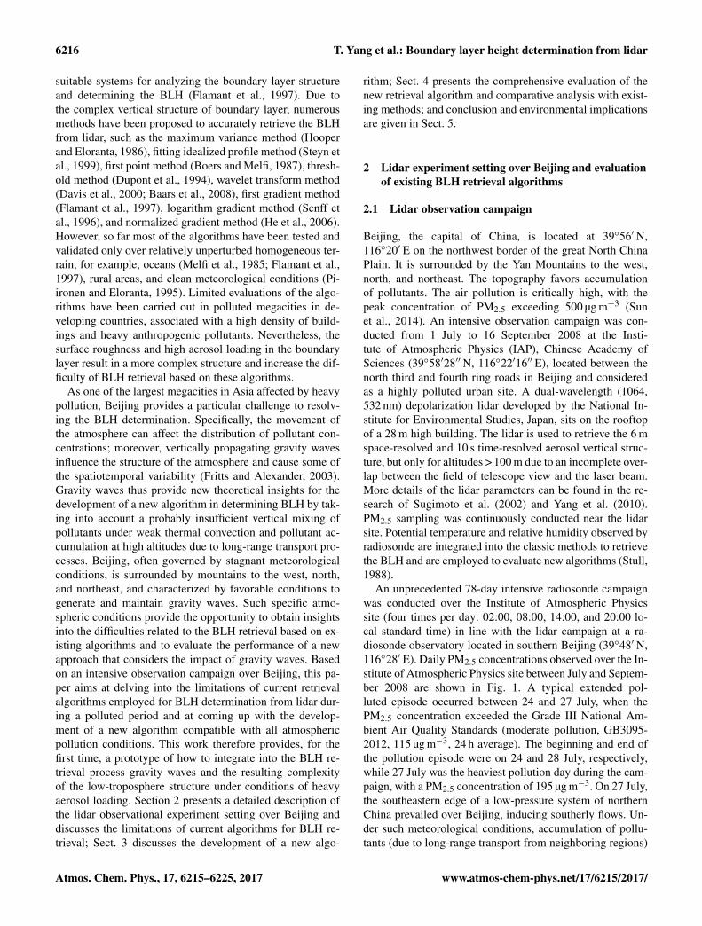
Figure 4b (similar to Fig. 2b) shows the BLH retrieved byCRGM as a red dotted line. Strong negative peaks were de-tected in the profiles for each algorithm to define the BLH(Fig. 4b). At 20:00 on 27 July, the BLH retrieved by CRGM

Table 1. Statistical parameters for each lidar retrieval algorithmcompared with radiosonde measurements.

CRGM GM LGM NGM

Correlation coefficient 0.91 0.71 0.50 0.44(R2)RMSE (m) 142 384 434 498

was 1350 m, in perfect agreement with the actual BLH de-termined by radiosonde (1350 m), as opposed to 480 and1590 m determined by LGM and NGM, respectively. The di-urnal cycles of the BLH retrieved by CRGM presented inFig. 4a show CRGM’s good capture of the unimodal diur-nal cycle of the BLH, presenting a peak at 14:00–15:00 anda valley at 07:00–08:00, induced by the thermal activity ofthe ground. In comparison with CRGM, the BLH determinedby LGM and NGM did not present unimodal diurnal cycles.On the other hand, although the GM-retrieved BLH showeda unimodal diurnal cycle, the amplitudes of the valley andpeak were lower. Comparing the four-moment radiosonde-retrieved BLH (02:00, 08:00, 14:00, 20:00) with the algo-rithms’ results highlights that CRGM presents the least bias,while GM shows an average underestimation of 500–600 m,and LGM and NGM result in an average overestimation of400–500 m. To enrich our analysis, a comparison of CRGMwith the other most frequently employed methods for BLHretrieval, such as the ideal curve fit (Steyn et al., 1999) andwavelet method (Davis et al., 2000), is provided in the Sup-plement (Figs. S4–S6). The result illustrates that fitting curveand wavelet methods also significantly underestimate BLHby approximately 600 and 800 m in maximum, respectively,during heavily polluted episodes in line with several otherprevious studies (Sawyer and Li, 2013; Wang et al., 2012; Suet al., 2017).

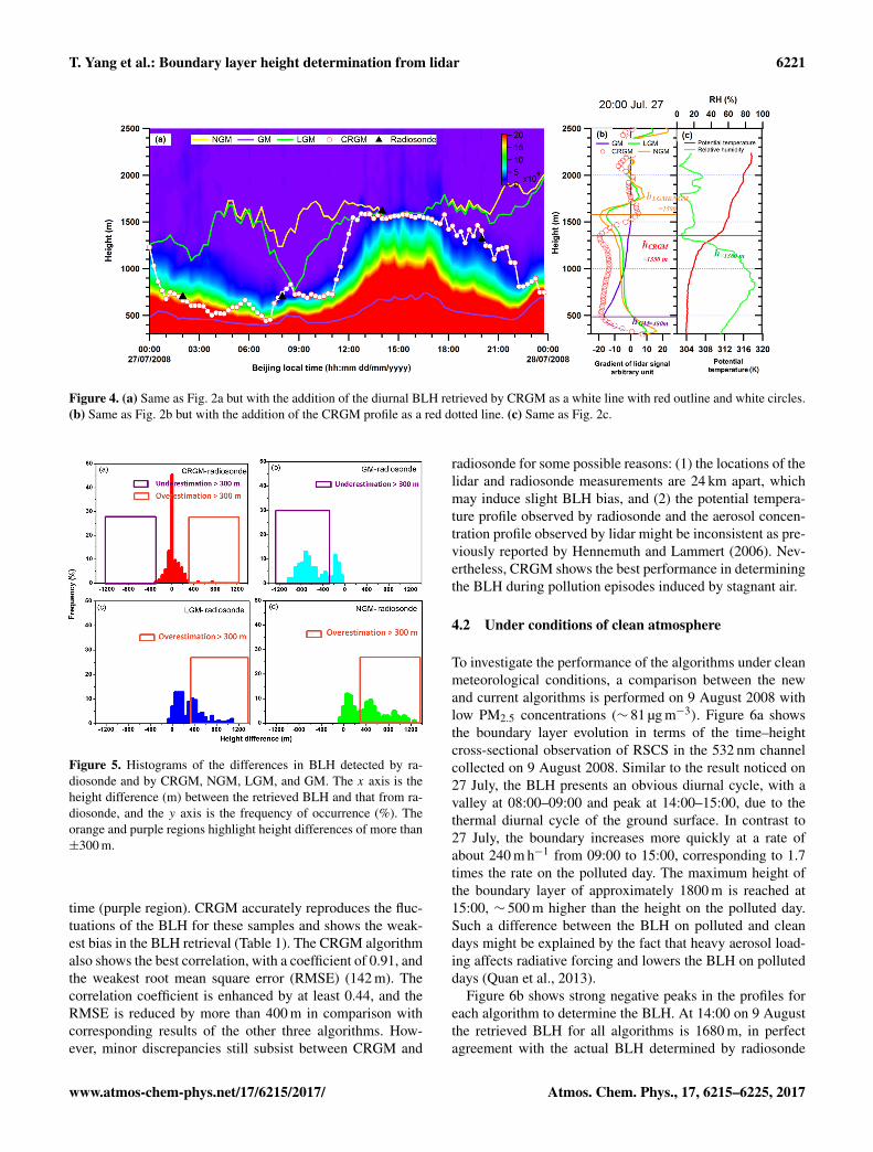
In order to further compare the performance of CRGMwith the current algorithms in heavily polluted episodes, theperiod of daily PM2.5 concentrations exceeding the GradeII National Ambient Air Quality Standards (light pollution,GB3095-2012, 75 µg m−3, 24 h average) is particularly ana-lyzed (in total 24 days). Radiosonde data of four correspond-ing times are used to evaluate retrieval algorithm results.Cloudy and rainy weather conditions are ignored to preventincrease of bias during the BLH retrieval process. There are89 available samples for each algorithm. Figure 5 presentsthe discrepancies between the retrieval algorithm results andthe radiosonde-detected BLH. Although the retrieval errorsare limited in CRGM, it shows slightly symmetric heightbias distribution of about 200 m. In contrast, the LGM andNGM retrievals significantly overestimate the BLH, with aheight bias range of 60–1110 m, exceeding 300 m for morethan 85 % of the measurements (orange region in Fig. 5). TheGM algorithm underestimates the BLH by 30–1140 m, withan underestimation of more than 300 m occurring 70 % of the

Atmos. Chem. Phys., 17, 6215–6225, 2017 www.atmos-chem-phys.net/17/6215/2017/

T. Yang et al.: Boundary layer height determination from lidar 6221

Figure 4. (a) Same as Fig. 2a but with the addition of the diurnal BLH retrieved by CRGM as a white line with red outline and white circles.(b) Same as Fig. 2b but with the addition of the CRGM profile as a red dotted line. (c) Same as Fig. 2c.

Figure 5. Histograms of the differences in BLH detected by ra-diosonde and by CRGM, NGM, LGM, and GM. The x axis is theheight difference (m) between the retrieved BLH and that from ra-diosonde, and the y axis is the frequency of occurrence (%). Theorange and purple regions highlight height differences of more than±300 m.

time (purple region). CRGM accurately reproduces the fluc-tuations of the BLH for these samples and shows the weak-est bias in the BLH retrieval (Table 1). The CRGM algorithmalso shows the best correlation, with a coefficient of 0.91, andthe weakest root mean square error (RMSE) (142 m). Thecorrelation coefficient is enhanced by at least 0.44, and theRMSE is reduced by more than 400 m in comparison withcorresponding results of the other three algorithms. How-ever, minor discrepancies still subsist between CRGM and

radiosonde for some possible reasons: (1) the locations of thelidar and radiosonde measurements are 24 km apart, whichmay induce slight BLH bias, and (2) the potential tempera-ture profile observed by radiosonde and the aerosol concen-tration profile observed by lidar might be inconsistent as pre-viously reported by Hennemuth and Lammert (2006). Nev-ertheless, CRGM shows the best performance in determiningthe BLH during pollution episodes induced by stagnant air.

4.2 Under conditions of clean atmosphere

To investigate the performance of the algorithms under cleanmeteorological conditions, a comparison between the newand current algorithms is performed on 9 August 2008 withlow PM2.5 concentrations (∼ 81 µg m−3). Figure 6a showsthe boundary layer evolution in terms of the time–heightcross-sectional observation of RSCS in the 532 nm channelcollected on 9 August 2008. Similar to the result noticed on27 July, the BLH presents an obvious diurnal cycle, with avalley at 08:00–09:00 and peak at 14:00–15:00, due to thethermal diurnal cycle of the ground surface. In contrast to27 July, the boundary increases more quickly at a rate ofabout 240 m h−1 from 09:00 to 15:00, corresponding to 1.7times the rate on the polluted day. The maximum height ofthe boundary layer of approximately 1800 m is reached at15:00, ∼ 500 m higher than the height on the polluted day.Such a difference between the BLH on polluted and cleandays might be explained by the fact that heavy aerosol load-ing affects radiative forcing and lowers the BLH on polluteddays (Quan et al., 2013).

Figure 6b shows strong negative peaks in the profiles foreach algorithm to determine the BLH. At 14:00 on 9 Augustthe retrieved BLH for all algorithms is 1680 m, in perfectagreement with the actual BLH determined by radiosonde

www.atmos-chem-phys.net/17/6215/2017/ Atmos. Chem. Phys., 17, 6215–6225, 2017

6222 T. Yang et al.: Boundary layer height determination from lidar

Figure 6. (a) Same as Fig. 4a but for 9 August. (b) Same as Fig. 4b but for 14:00 on 9 August. (c) Same as Fig. 4c but for 14:00 on 9 August.

Figure 7. Comparison of HCRGM, HGM, HLGM, and HNGM with the BLH retrieved from radiosonde measurements. The x axis shows theradiosonde retrieval, and the y axis is the lidar retrieval using the different algorithms. The solid line indicates y = x. (a) CRGM, (b) GM,(c) LGM, (d) NGM. Different marks represent the comparisons under different pollution conditions (PM2.5 concentrations). The comparisonsunder PM2.5 concentrations less than 35, 35–75, 75–115, 115–150, and 150–250 µg m−3 are shown as green circles, yellow triangles, browntriangles, red diamonds, and purple hexagons, respectively.

(1680 m). All diurnal cycle results converge at 14:00 on 9August, demonstrating that all retrieval algorithms capturethe overall diurnal cycle of the actual BLH. Comparison ofCRGM with existing ideal curve fit and wavelet methodsalso confirms such performance (Fig. S7). Such good per-formance of all the algorithms under clean meteorologicalconditions is a result of the homogenous vertical distribu-tion of aerosols, since under clean conditions, mixing of theaerosols by strong thermal convection is more sufficient dueto weak pollutant loading. In addition, there is no obviouslarge negative gradient peak to disturb the determination ofthe BLH.

4.3 At various pollution levels

Under various air pollution conditions (all pollution levels),a total of 298 radiosondes measurements are analyzed toestimate the BLH with comparison to retrieval algorithms.Cases of nocturnal BLH below the useful lidar signal (before

Table 2. Root mean square error (RMSE) for each lidar retrievalmethod compared with radiosonde measurements and sample sizein each comparison level.

PM2.5 CRGM GM LGM NGM Samples(µg m−3) (m) (m) (m) (m)

0–35 124 124 137 129 11435–75 123 133 238 227 8875–115 135 213 320 418 53115–150 154 310 346 434 19150–250 137 629 636 643 24

the overlap reaches 1) or thin cumulus cloud formations atthe upper boundary layer (resulting in large error in the re-trieval) are neglected. The cloud and rain detection followsthe methods employed by the Asian Dust and Aerosol Li-dar Observation Network (AD-net) in East Asia, supported

Atmos. Chem. Phys., 17, 6215–6225, 2017 www.atmos-chem-phys.net/17/6215/2017/

T. Yang et al.: Boundary layer height determination from lidar 6223

by the World Meteorological Organization (WMO) GlobalAtmosphere Watch (GAW) program. Rain was detected bycolor ratio (γ ′, the ratio of β ′1064 to β ′532) to distinguishrainy and clear (no rain) regions, in which β ′1064 and β ′532present the attenuated backscatter coefficient at 1064 and532 nm, respectively. Large droplets have a large γ ′ value,so once γ ′ exceeds a threshold (1.1) over a certain verticalinternal in the lower atmosphere, the profile is classified asa rain profile. Cloud base height is determined by the ver-tical gradient of β ′1064 and the peak value of β ′1064 betweenthe cloud base and the apparent cloud top. A detailed de-scription of the method is provided by Shimizu et al. (2016).The 298 samples are categorized into five groups accordingto the corresponding hourly PM2.5 concentration. We com-pare retrieved BLH by the algorithms from lidar with the ra-diosonde results in each group. As illustrated in Fig. 7, theretrieval results of CRGM are close to the 1 : 1 line, whilethe GM, LGM, and NGM present large biases. The GM re-sults are generally below the 1 : 1 line, highlighting an un-derestimation of the BLH. LGM and NGM in general over-estimate the BLH in all five comparison groups. The RMSEranges over 124–137 m for CRGM, as opposed to 124–642 mfor the other three algorithms. Furthermore, the RMSE ofthe three existing algorithms increases with the PM2.5 con-centrations (Table 2). For the GM algorithm, the RMSE in-creases from 124 to 629 m with an increase of PM2.5 con-centration from 35 to 250 µg m−3. Similarly, the RMSE ofLGM and NGM increases from∼ 130 to 540 m with a PM2.5concentration increase from 35 to 250 µg m−3. High aerosolloading is therefore always associated with higher RMSE.In contrast, the RMSE of CRGM remains relatively constantwith the changes of air pollution level. These results perfectlycorroborate the findings discussed in Sect. 4.1 and 4.2. It isclear that existing retrieval algorithms are only suitable to theaerosol profiles similar to the “textbook” boundary layer de-velopment, while CRGM appears to be a robust techniquefor BLH determination by lidar.

5 Conclusions and environmental implication

Lidar is an appropriate instrument with which to determinethe boundary layer height with high temporal and verticalresolution. In this paper, an intensive lidar observation cam-paign was conducted in Beijing to thoroughly evaluate thelimitations of the current method for boundary layer heightdetermination and develop an algorithm suitable to all pollu-tion conditions. Incontestably, current commonly employedretrieval algorithms (first gradient method, logarithm gra-dient method, and normalized gradient method) are unableto determine the boundary layer height during heavily pol-luted episodes due to inhomogeneous vertical distribution ofaerosols under stable meteorological conditions associatedwith the impact of vertically propagating gravity waves onthe tropospheric structure. The gradient algorithm critically

underestimates the boundary layer height by 30–1140 m,with an underestimation higher than 300 m occurring 70 %of the time. The logarithm and normalized gradient meth-ods overestimate the boundary layer height, exceeding 300 mmore than 85 % of the time.

The newly developed method (the cubic root gradient)considers the linear instability theory of gravity waves to de-termine the boundary layer height by capturing the verticalmovement of aerosol at the transition between waves and tur-bulence. As a result, the cubic root gradient method describesthe fluctuation of the boundary layer with the best correlation(R2= 0.91) and the weakest RMSE (142 m) under various

atmospheric pollution conditions. In comparison with currentgradient methods, the new technique reduces the RMSE by400 m minimum under all pollution conditions. The RMSEof existing retrieval algorithms typically varies with aerosolloading (high RMSE is always associated with heavy aerosolloading, and weak RMSE correlates with weak aerosol load-ing), while the RMSE of the new method remains almostconstant with the changes of air pollution levels. The cubicroot gradient method appears therefore to be a robust tech-nique for boundary layer height determination from lidar.

In terms of environmental implication, such innovationwould technically contribute to improving the accuracy of re-gionally spatiotemporal distribution models and forecasts ofaerosol loadings for an effective pollution control measure, inparticular over a number of megacities in China, since accu-rately determining the boundary layer is one of the importantfactors of uncertainties and bias reduction for reasonable airpollution modeling and forecasts. However, further develop-ment and expansion of lidar observation system are needednotably under cloudy and rainy conditions in order to providea greater benefit to pollution control management.

Data availability. Contact Ting Yang (tingyang@mail.iap.ac.cn)for data requests.

The Supplement related to this article is available onlineat doi:10.5194/acp-17-6215-2017-supplement.

Competing interests. The authors declare that they have no conflictof interest.

Acknowledgements. This work was supported by the NaturalNational Science Foundation of China (NSFC) (41305115,41225019), Program 973 (2014CB447900), the CommonwealProject of the Ministry of Environmental Protection (201409001),and Program 863 (2014AA06AA06A512). Ting Yang is gratefulfor the invaluable emotional support received from her fam-ily over the years to overcome all the periods of darkness, andthe endless happiness and courage received from her baby daughter.

www.atmos-chem-phys.net/17/6215/2017/ Atmos. Chem. Phys., 17, 6215–6225, 2017

6224 T. Yang et al.: Boundary layer height determination from lidar

Edited by: F. YuReviewed by: three anonymous referees

References

Ansari, A. S., and Pandis, S. N.: Response of inorganic PM to pre-cursor concentrations, Environ. Sci. Technol., 32, 2706–2714,1998.

Baars, H., Ansmann, A., Engelmann, R., and Althausen, D.: Con-tinuous monitoring of the boundary-layer top with lidar, At-mos. Chem. Phys., 8, 7281–7296, doi:10.5194/acp-8-7281-2008,2008.

Boers, R. and Melfi, S. H.: Cold air outbreak during MASEX: Lidarobservations and boundary-layer model test, Bound.-Lay. Mete-orol., 39, 41–51, doi:10.1007/bf00121864, 1987.

Chan, C. K. and Yao, X.: Air pollution in mega cities in China,Atmos. Environ., 42, 1–42, doi:10.1016/j.atmosenv.2007.09.003,2008.

Dabberdt, W. F., Carroll, M. A., Baumgardner, D., Carmichael, G.,Cohen, R., Dye, T., Ellis, J., Grell, G., Grimmond, S., Hanna, S.,Irwin, J., Lamb, B., Madronich, S., McQueen, J., Meagher, J.,Odman, T., Pleim, J., Schmid, H. P., and Westphal, D. L.: Meteo-rological Research Needs for Improved Air Quality Forecasting:Report of the 11th Prospectus Development Team of the U.S.Weather Research Program*, B. Am. Meteorol. Soc., 85, 563–586, doi:10.1175/bams-85-4-563, 2004.

Dandou, A., Tombrou, M., Schäfer, K., Emeis, S., Protonotar-iou, A. P., Bossioli, E., Soulakellis, N., and Suppan, P.: AComparison Between Modelled and Measured Mixing-LayerHeight Over Munich, Bound-Lay. Meteorol., 131, 425–440,doi:10.1007/s10546-009-9373-7, 2009.

Davis, K. J., Gamage, N., Hagelberg, C. R., Kiemle, C., Lenschow,D. H., and Sullivan, P. P.: An Objective Method for Deriv-ing Atmospheric Structure from Airborne Lidar Observations,J. Atmos. Oceanic Technol., 17, 1455–1468, doi:10.1175/1520-0426(2000)017<1455:aomfda>2.0.co;2, 2000.

Dewan, E. M. and Good, R. E.: Saturation and the “universal” spec-trum for vertical profiles of horizontal scalar winds in the atmo-sphere, J. Geophys. Res.-Atmos., 91, 2742–2748, 1986.

Dupont, E., Pelon, J., and Flamant, C.: Study of the moist Convec-tive Boundary Layer structure by backscattering lidar, Bound.-Lay. Meteorol., 69, 1–25, doi:10.1007/bf00713292, 1994.

Emeis, S., Jahn, C., Munkel, C., Munsterer, C., and Schafer, K.:Multiple atmospheric layering and mixing-layer height in he Innvalley observed by remote sensing, Meteorol. Z., 16, 415–424,2007.

Fernald, F. G.: Analysis of atmospheric lidar observations – Somecomments, Appl. Opt., 23, 652–653, 1984.

Flamant, C., Pelon, J., Flamant, P., and Durand, P.: Lidar Determina-tion Of The Entrainment Zone Thickness At The Top Of The Un-stable Marine Atmospheric Boundary Layer, Bound.-Lay. Mete-orol., 83, 247–284, doi:10.1023/a:1000258318944, 1997.

Fritts, D. C. and Alexander, M. J.: Gravity wave dynamics and ef-fects in the middle atmosphere, Rev. Geophys., 41, 1003–1066,doi:10.1029/2001rg000106, 2003.

Gardner, C. S.: Testing theories of atmospheric gravity wave satura-tion and dissipation, J. Atmos. Terr. Phys., 58, 1575–1589, 1996.

Gibert, F., Arnault, N., Cuesta, J., Plougonven, R., and Flamant, P.H.: Internal gravity waves convectively forced in the atmosphericresidual layer during the morning transition, Q. J. Roy. Meteor.Soc., 137, 1610–1624, doi:10.1002/qj.836, 2011.

Gong, S., Yang, G., Xu, J., Wang, J., Guan, S., Gong, W.,and Fu, J.: Statistical characteristics of atmospheric gravitywave in the mesopause region observed with a sodium li-dar at Beijing, China, J. Atmos. Sol.-Terr. Phy., 97, 143–151,doi:10.1016/j.jastp.2013.03.005, 2013.

Hayden, K. L., Anlauf, K. G., Hoff, R. M., Strapp, J. W., Bot-tenheim, J. W., Wiebe, H. A., Froude, F. A., Martin, J. B.,Steyn, D. G., and McKendry, I. G.: The vertical chemical andmeteorological structure of the boundary layer in the LowerFraser Valley during Pacific ’93, Atmos. Environ., 31, 2089–2105, doi:10.1016/S1352-2310(96)00300-7, 1997.

He, Q. S., Mao, J. T., Chen, J. Y., and Hu, Y. Y.: Observational andmodeling studies of urban atmospheric boundary-layer heightand its evolution mechanisms, Atmos. Environ., 40, 1064–1077,doi:10.1016/j.atmosenv.2005.11.016, 2006.

Hennemuth, B. and Lammert, A.: Determination of the At-mospheric Boundary Layer Height from Radiosonde andLidar Backscatter, Bound.-Lay. Meteorol., 120, 181–200,doi:10.1007/s10546-005-9035-3, 2006.

Hooper, W. P. and Eloranta, E. W.: Lidar measurements of wind inthe planetary borendary layer: the method, accuracy and resultsfrom joint measurement with radiosonde and kytoon, Am. Mete-orol. Soc., 25, 990–1001, 1986.

Melfi, S., Spinhirne, J., Chou, S., and Palm, S.: Lidar observa-tions of vertically organized convection in the planetary bound-ary layer over the ocean, J. Clim. Appl. Meteorol., 24, 806–821,1985.

Pal, S., Behrendt, A., and Wulfmeyer, V.: Elastic-backscatter-lidar-based characterization of the convective boundary layer and in-vestigation of related statistics, Ann. Geophys., 28, 825–847,2010.

Park, O. H., Seo, S. J., and Lee, S. H.: Laboratory Sim-ulation Of Vertical Plume Dispersion Within A Convec-tive Boundary Layer, Bound.-Lay. Meteorol., 99, 159–169,doi:10.1023/a:1018731205971, 2001.

Piironen, A. K. and Eloranta, E. W.: Convective boundary layermean depths and cloud geometrical properties obtained from vol-ume imaging lidar data, J. Geophys. Res.-Atmos., 100, 25569–25576, doi:10.1029/94jd02604, 1995.

Quan, J., Gao, Y., Zhang, Q., Tie, X., Cao, J., Han, S.,Meng, J., Chen, P., and Zhao, D.: Evolution of planetaryboundary layer under different weather conditions, and itsimpact on aerosol concentrations, Particuology, 11, 34–40,doi:10.1016/j.partic.2012.04.005, 2013.

Sawyer, V. and Li, Z.: Detection, variations and intercompari-son of the planetary boundary layer depth from radiosonde, li-dar and infrared spectrometer, Atmos. Environ., 79, 518–528,doi:10.1016/j.atmosenv.2013.07.019, 2013.

Seibert, P., Beyrich, F., Gryning, S.-E., Joffre, S., Rasmussen, A.,and Tercier, P.: Review and intercomparison of operational meth-ods for the determination of the mixing height, Atmos. Environ.,34, 1001–1027, doi:10.1016/S1352-2310(99)00349-0, 2000.

Senff, C., Bösenberg, J., Peters, G., and Schaberl, T.: Remote sens-ing of turbulent ozone fluxes and the ozone budget in the convec-

Atmos. Chem. Phys., 17, 6215–6225, 2017 www.atmos-chem-phys.net/17/6215/2017/

T. Yang et al.: Boundary layer height determination from lidar 6225

tive boundary layer with DIAL and radar-RASS: a case study,Contributions Atmos. Phys., 69, 161–176, 1996.

Shimizu, A., Nishizawa, T., Jin, Y., Kim, S.-W., Wang, Z., Batdorj,D., and Sugimoto, N.: Evolution of a lidar network for tropo-spheric aerosol detection in East Asia, OPTICE, 56, 031219–031219, doi:10.1117/1.OE.56.3.031219, 2016.

Sicard, M., Pérez, C., Rocadenbosch, F., Baldasano, J. M., andGarcía-Vizcaino, D.: Mixed-Layer Depth Determination in theBarcelona Coastal Area From Regular Lidar Measurements:Methods, Results and Limitations, Bound.-Lay. Meteorol., 119,135–157, doi:10.1007/s10546-005-9005-9, 2006.

Stettler, M. and Hoyningen-Huene, W.: On the relation betweenhaze layer and air mass aerosol at an urban location – Case stud-ies, Atmos. Res., 40, 1–18, doi:10.1016/0169-8095(95)00029-1,1996.

Steyn, D. G., Baldi, M., and Hoff, R. M.: The Detection ofMixed Layer Depth and Entrainment Zone Thickness from LidarBackscatter Profiles, J. Atmos. Ocean. Technol., 16, 953–959,1999.

Stull, R. B.: An introduction to boundary layer meteorology,Springer, 1988.

Su, T., Li, J., Li, C., Xiang, P., Lau, A. K.-H., Guo, J., Yang, D., andMiao, Y.: An intercomparison of long-term planetary boundarylayer heights retrieved from CALIPSO, ground-based lidar andradiosonde measurements over Hong Kong, J. Geophys. Res.-Atmos., 122, 3929–3943, doi:10.1002/2016jd025937, 2017.

Sugimoto, N., Matsui, I., Shimizu, A., Uno, I., Asai, K., Endoh, T.,and Nakajima, T.: Observation of dust and anthropogenic aerosolplumes in the Northwest Pacific with a two-wavelength polariza-tion lidar on board the research vessel Mirai, Geophys. Res. Lett.,29, 1901, doi:10.1029/2002gl015112, 2002.

Sun, Y., Jiang, Q., Wang, Z., Fu, P., Li, J., Yang, T., and Yin, Y.: In-vestigation of the sources and evolution processes of severe hazepollution in Beijing in January 2013, J. Geophys. Res.-Atmos.,119, 4380–4398, doi:10.1002/2014jd021641, 2014.

Tie, X., Madronich, S., Li, G., Ying, Z., Zhang, R., Garcia, A.R., Lee-Taylor, J., and Liu, Y.: Characterizations of chemi-cal oxidants in Mexico City: A regional chemical dynamicalmodel (WRF-Chem) study, Atmos. Environ., 41, 1989–2008,doi:10.1016/j.atmosenv.2006.10.053, 2007.

Wang, D. Y., Ward, W. E., Solheim, B. H., and Shepherd, G. G.:Wavenumber spectra of horizontal wind and temperature mea-sured with WINDII, Part II: diffusive effect on spectral forma-tion, J. Atmos. Sol.-Terr. Phy., 62, 981–991, doi:10.1016/S1364-6826(00)00065-1, 2000.

Wang, Z., Cao, X., Zhang, L., Notholt, J., Zhou, B., Liu, R.,and Zhang, B.: Lidar measurement of planetary boundary layerheight and comparison with microwave profiling radiometer ob-servation, Atmos. Meas. Tech., 5, 1965–1972, doi:10.5194/amt-5-1965-2012, 2012.

Yang, T., Wang, Z., Zhang, B., Wang, X., Wang, W., Gbauidi, A.,and Gong, Y.: Evaluation of the effect of air pollution control dur-ing the Beijing 2008 Olympic Games using Lidar data, Chin. Sci.Bull., 55, 1311–1316, doi:10.1007/s11434-010-0081-y, 2010.

www.atmos-chem-phys.net/17/6215/2017/ Atmos. Chem. Phys., 17, 6215–6225, 2017