Technical note: A h igh -resolution inverse modelling

1

Technical note: A high-resolution inverse modelling technique for

estimating surface CO2 fluxes based on the NIES-TM - FLEXPART

coupled transport model and its adjoint.

Shamil Maksyutov1, Tomohiro Oda2, Makoto Saito1, Rajesh Janardanan1, Dmitry Belikov1,3, Johannes 5

W. Kaiser4, Ruslan Zhuravlev5, Alexander Ganshin5, Vinu K. Valsala6, Arlyn Andrews7, Lukasz

Chmura8, Edward Dlugokencky7, László Haszpra9, Ray L. Langenfelds10, Toshinobu Machida1,

Takakiyo Nakazawa11, Michel Ramonet12, Colm Sweeney7, Douglas Worthy13

1National Institute for Environmental Studies, Tsukuba, Japan 10 2NASA Goddard Space Flight Center, Greenbelt, MD, USA/Universities Space Research Association, Columbia, MD,

USA 3now at Chiba University, Chiba, Japan 4Deutscher Wetterdienst, Offenbach, Germany 5Central Aerological Observatory, Dolgoprudny, Russia 15 6Indian Institute for Tropical Meteorology, Pune, India 7Earth System Research Laboratory, NOAA, Boulder, CO, USA 8AGH University of Science and Technology, Krakow, Poland 9Research Centre for Astronomy and Earth Sciences, Sopron, Hungary 10Climate Science Centre, CSIRO Oceans and Atmosphere, Aspendale, VIC, Australia 20 11Tohoku University, Sendai, Japan 12Laboratoire des Sciences du Climat et de l’Environnement, LSCE-IPSL, Gif-sur-Yvette, France 13Environment and Climate Change Canada, Toronto, Canada

Correspondence to: S. Maksyutov ([email protected])

Abstract 25

We developed a high-resolution surface flux inversion system based on the global Lagrangian-Eulerian coupled tracer

transport model composed of National Institute for Environmental Studies Transport Model (NIES-TM) and FLEXible

PARTicle dispersion model (FLEXPART). The inversion system is named NTFVAR (NIES-TM-FLEXPART-variational)

as it applies variational optimisation to estimate surface fluxes. We tested the system by estimating optimized corrections

to natural surface CO2 fluxes to achieve best fit to atmospheric CO2 data collected by the global in-situ network, as a 30

necessary step towards capability of estimating anthropogenic CO2 emissions. We employ the Lagrangian particle

dispersion model (LPDM) FLEXPART to calculate the surface flux footprints of CO2 observations at a 0.1° × 0.1° spatial

https://doi.org/10.5194/acp-2020-251Preprint. Discussion started: 27 March 2020c© Author(s) 2020. CC BY 4.0 License.

2

resolution. The LPDM is coupled to a global atmospheric tracer transport model (NIES-TM). Our inversion technique uses

an adjoint of the coupled transport model in an iterative optimization procedure. The flux error covariance operator is being

implemented via implicit diffusion. Biweekly flux corrections to prior flux fields were estimated for the years 2010-2012

from in-situ CO2 data included in the Observation Package (ObsPack) dataset. High-resolution prior flux fields were

prepared using Open-Data Inventory for Anthropogenic Carbon dioxide (ODIAC) for fossil fuel combustion, Global Fire 5

Assimilation System (GFAS) for biomass burning, the Vegetation Integrative SImulator for Trace gases (VISIT) model

for terrestrial biosphere exchange and Ocean Tracer Transport Model (OTTM) for oceanic exchange. The terrestrial

biospheric flux field was constructed using a vegetation mosaic map and separate simulation of CO2 fluxes at daily time

step by the VISIT model for each vegetation type. The prior flux uncertainty for terrestrial biosphere was scaled

proportionally to the monthly mean Gross Primary Production (GPP) by the Moderate Resolution Imaging 10

Spectroradiometer (MODIS) MOD17 product. The inverse system calculates flux corrections to the prior fluxes in the form

of a relatively smooth field multiplied by high-resolution patterns of the prior flux uncertainties for land and ocean,

following the coastlines and vegetation productivity gradients. The resulting flux estimates improve fit to the observations

at continuous observations sites, reproducing both the seasonal variation and short-term concentration variability, including

high CO2 concentration events associated with anthropogenic emissions. The use of high-resolution atmospheric transport 15

in global CO2 flux inversion has the advantage of better resolving the transport from the mix of the anthropogenic and

biospheric sources in densely populated continental regions and shows potential for better separation between fluxes from

terrestrial ecosystems and strong localised sources such as anthropogenic emissions and forest fires. Further improvements

in the modelling system are needed as the posterior fit is better than that by the National Oceanic and Atmospheric

Administration (NOAA) CarbonTracker only for a fraction of the monitoring sites, mostly at coastal and island locations 20

experiencing mix of background and local flux signals.

1 Introduction

Inverse modelling of the surface fluxes is implemented by using chemical transport model simulations to match

atmospheric observations of greenhouse gases. CO2 flux inversions studies started from addressing large scale flux 25

distributions (Enting and Mansbridge, 1989; Tans et al., 1990; Gurney et al., 2002; Peylin et al., 2013 and others) using

background monitoring data and global transport models at low and medium resolutions targeting extraction of the

information on large and highly variable fluxes of carbon dioxide from terrestrial ecosystems and oceans. Merits of

improving the resolutions of global transport simulations to 9-25 km have been also discussed by previous studies, such as

Agusti-Panareda et al. (2019) and Maksyutov et al. (2008). However, global inverse modelling studies have never been 30

conducted at these spatial resolutions. On the other hand, regional scale fluxes, such as national emissions of non-CO2


3

greenhouse gases (GHGs), have been estimated using inverse modelling tools relying on regional (mostly Lagrangian)

transport algorithms capable of resolving surface flux contributions to atmospheric concentrations at resolutions from 1 to

100 km (Vermeulen et al., 1999; Manning et al., 2011; Stohl et al., 2009; Rodenbeck et al., 2009; Henne et al., 2016; He

et al., 2018; Schuh et al., 2013; Lauvaux et al., 2016 and others). Extension of the regional Lagrangian inverse modelling

to the global scale based on combination of three-dimensional (3-D) global Eulerian model and Lagrangian model have 5

been implemented in several studies (Rugby et al., 2011; Zhuravlev et al., 2013; Shirai et al., 2017), which demonstrated

an enhanced capability of resolving the regional and local concentration variability driven by fine scale surface emission

patterns, while using inverse modeling schemes relying on regional and global basis functions that yield concentration

responses of regional fluxes at observational sites. A disadvantage of using regional basis functions in inverse modeling is

the flux aggregation errors as noted by Kaminski et al. (2001), is addressed by developing grid-based inversion schemes 10

based on variational assimilation algorithms that yield flux corrections that are not tied to aggregated flux regions

(Rodenbeck et al., 2003; Chevallier et al., 2005; Baker et al., 2006, and others). In order to implement a grid-based inversion

scheme suitable for optimizing surface fluxes using a high-resolution atmospheric transport capability of the Lagrangian

model, an adjoint of a coupled Eulerian-Lagrangian model is needed, such as one reported by Belikov et al. (2016).

In thus study, we applied an adjoint of the coupled Eulerian-Lagrangian transport model, which is a revised version of 15

Belikov et al. (2016), to the problem of surface flux inversion based on transport model with spatial resolution of 0.1°

longitude-latitude. While global higher resolution transport runs, such as ~1 km, can be done with coupled Eulerian-

Lagrangian models (Ganshin et al., 2012), the choice of the model resolution in our inversion system is often dictated

mainly by the availability of the prior surface CO2 fluxes and the size of available computer memory. A practical need for

running high-resolution atmospheric transport simulations at global scale is currently driven by expanding GHG observing 20

capabilities towards quantifying anthropogenic emissions by observing at the vicinity of emission sources (Nassar et al.,

2017), including observations in both background and urban sites, with tall towers, commercial airplanes, and satellites.

At the same time, the focus of inverse modeling is evolving towards studies of the anthropogenic emissions, with a target

of making better estimates of regional and national emissions in support of national and regional GHG emission reporting

and control measures (Manning et al., 2011; Henne et al., 2016; Lauvaux et al., 2016). In that context, global-scale high-25

resolution inverse modeling approaches have advantage in closing global budgets, while regional and national scale inverse

modeling approaches with limited area models require boundary conditions normally provided by global model simulations

with optimized fluxes. Often there is an additional degree of freedom introduced by allowing corrections to the boundary

concentration distribution to improve a fit at the observation sites (Manning et al., 2011). As a result, the global total of

regional emission estimates does not necessarily match the balance constrained by global mean concentration trends. A 30

global coupled Eulerian-Lagrangian model (e.g. Ganshin et al., 2012), has potential for addressing both the objectives, that


4

is closing the global balance and operating at range of scales from a single city (Lauvaux et al., 2016) to large country or

continental scale. Here we report developing a high-resolution inverse modeling technique suitable for application at a

broad range of spatial scales and apply it to the problem of estimating the distribution of CO2 fluxes over the globe that

provides best fit to the observations. In separate studies, the same inversion systems were applied to inverse modeling of

methane emissions (Wang et al., 2019; Janardanan et al., 2020). 5

In this paper, we report its application to the inverse problem of the natural CO2 flux estimation as a first step towards

estimating the fossil CO2 emissions where the advantage of high-resolution approach is more evident. The paper is

composed as follows: this Section 1 provides Introduction; Section 2, the transport model and its adjoint; Section 3

introduces the Prior fluxes, observational dataset, and gridded flux uncertainties; Section 4 gives the formulation of the

inverse modeling problem and numerical solution; Section 5 presents simulation results and discussion, which is followed 10

by the Summary and Conclusions.

2 The coupled tracer transport model, its adjoint and the implementation

For simulation of the CO2 transport in the atmosphere we used a coupled Eulerian-Lagrangian model NIES-TM-15

FLEXPART, which is a further modification of the model described by Belikov et al. (2016). The coupled model combines

NIES-TM v08.1i with horizontal resolution of 2.5° × 2.5° and 32 hybrid-isentropic vertical levels (Belikov et al., 2013)

and FLEXPART model v.8.0 (Stohl et al., 2005) run in backward mode with surface flux resolution of 0.1° × 0.1°. Both

models use the Japan 25-year reanalysis (JRA-25)/JMA Climate Data Assimilation System (JCDAS) meteorology (Onogi

et al., 2007), with 40 vertical levels interpolated to a 1.25° × 1.25° grid. The use of low-resolution wind fields for high 20

resolution transport is better justified for cases of nearly geostrophic flow over flat terrain (Ganshin et al., 2012), but was

also considered applicable in regions with more complex topography (Ware et al., 2019). The coupled transport model

adjoint was derived from the Global Eulerian-Lagrangian Coupled Atmospheric transport model (GELCA) (Ganshin et al.,

2012; Zhuravlev et al., 2013; Shirai et al., 2017). To facilitate model application in our iterative inversion algorithm, all

the components of the model – Eulerian model and the coupler are integrated in one executable (online coupling) as 25

described in Belikov et al., (2016), while the original GELCA model implements Eulerian and Lagrangian components

sequentially, and then applies the coupler (off-line coupling). The changes in the current version with respect to the version

presented by Belikov et al. (2016) include an adjoint code derivation for model components using the adjoint code compiler

Tapenade (Hascoet and Pascual, 2013), instead of using the TAF compiler (Giering and Kaminski, 2003). Additionally,

the indexing and sorting algorithms for the transport matrix were revised to allow an efficient memory use for processing 30

large matrices of LPDM-driven responses to surface fluxes arising in the case of high-resolution surface fluxes and large


5

number of observations, especially when using satellite data. A manually derived adjoint of the NIES-TM v08.1i is used

as in Belikov et al. (2016), due to its computational efficiency. In the version of the model that includes manually coded

adjoint, only the second order van Leer algorithm (van Leer, 1977) is implemented, as opposed to third order algorithm

typically used in forward model (Belikov et al., 2013).

5

3 Prior fluxes, flux uncertainties and observations

Prior CO2 fluxes, were prepared as a combination of monthly-varying fossil fuel emissions by the Open-Data Inventory

for Anthropogenic Carbon dioxide (ODIAC), available at a global 30 arc second resolution (Oda et al., 2018), ocean-10

atmosphere exchange by the Ocean Tracer Transport Model (OTTM) 4D-var assimilation system, available at a 1°

resolution (Valsala and Maksyutov, 2010), daily CO2 emissions by biomass burning by Global Fire Assimilation System

(GFAS) dataset provided by Copernicus services at a 0.1° resolution (Kaiser et al., 2012), and daily varying climatology

of terrestrial biospheric CO2 exchange simulated by optimized Vegetation Integrative SImulator for Trace gases (VISIT)

model (Ito, 2010; Saito et al., 2014). Figure 1 presents samples of the four prior flux components (fossil, vegetation, 15

biomass burning and ocean) used in the forward simulation.

3.1 Emissions from fossil fuel

For fossil fuel CO2 emissions (emissions due to of fossil fuel combustion and cement manufacturing) we used ODIAC data

product (Oda and Maksyutov, 2011, 2015; Oda et al., 2018) at 0.1° × 0.1° resolution on monthly basis. The version 2016

of the ODIAC-2016 data product (ODIAC2016, Oda et al., 2018) is based on global and national emission estimates and 20

monthly estimates made at monthly resolution by the Carbon Dioxide Information Analysis Center (CDIAC) (Boden et

al., 2016; Andres et al., 2011). For spatial disaggregation it uses the emission data for powerplant emissions by the CARbon

Monitoring and Action (CARMA) database (Wheeler and Ummel, 2008), while the rest of the national total emissions on

land were distributed using spatial patterns provided by night-time lights data collected by the Defence Meteorological

Satellite Program (DMSP) satellites (Elvidge et al., 1999). The ODIAC fluxes were aggregated to a 0.1° resolution from 25

the high-resolution ODIAC data. The ODIAC emission product is suitable for this type of studies because the global total

emission is constrained by updated estimates while providing a high-resolution emission estimate. Thus, it can be applied

to carbon budget problems across different scales.


6

3.2 Terrestrial biosphere fluxes

CO2 fluxes by the terrestrial biosphere at a resolution of 0.1° were constructed using a vegetation mosaic approach,

combining the vegetation map data by synergetic land cover product (SYNMAP) dataset (Jung et al., 2006), available at a

30 arc second resolution, with terrestrial biospheric CO2 exchanges simulated by optimized VISIT model (Saito et al.,

2014) for each vegetation type in every 0.5° grid at daily time step. The area fraction of each vegetation type is derived 5

from SYNMAP data for each 0.1° grid. The CO2 net ecosystem exchange (NEE) fluxes on 0.1° grid were prepared by

combining the vegetation type-specific fluxes with vegetation area fraction data on 0.1° grid. By averaging the daily flux

data for period of 2000-2005 the flux climatology was derived for use in the recent years, when the VISIT model simulation

based on JRA-25-JCDAS reanalysis data is not available.

3.3 Emissions from biomass burning 10

Daily biomass burning CO2 emissions by Global Fire Assimilation System (GFAS) dataset relies on assimilating Fire

Radiative Power (FRP) observations from the MODIS instruments onboard the Terra and Aqua satellites (Kaiser et al.,

2012). The fire emissions at 0.1° resolution are calculated from FRP with land cover-specific conversion factors compiled

from a literature survey. The GFAS system adds corrections for observation gaps in the observations, and filters spurious

FRP observations of volcanoes, gas flares and other sources. 15

3.4 Oceanic exchange flux

The air-sea CO2 flux component for the flux inversion used an optimized estimate of oceanic CO2 fluxes by Valsala and

Maksyutov (2010). The dataset is constructed with a variational assimilation of the observed partial pressure of surface

ocean CO2 (pCO2) available in Takahashi et al. (2017) database into the OTTM (Valsala et al., 2008), coupled with a

simple one-component ecosystem model. The assimilation consists of a variational optimization method which minimizes 20

the model to observation differences in the surface ocean dissolved inorganic carbon (DIC) (or pCO2) within two-month

time window. The OTTM model fluxes produced on a 1° × 1° grid at monthly time step are interpolated to a 0.1° × 0.1°

grid, taking into account, the land fraction map derived from 1 km resolution MODIS landcover product.

3.5 Flux uncertainties for land and ocean.

CO2 flux uncertainties are needed for both land and ocean. Climatological, monthly-varying flux uncertainties for land 25

were set to 20% of MODIS gross primary productivity (GPP) by MOD17A2 product available on a 0.05° grid at monthly


7

resolution (Running et al., 2004). Oceanic flux uncertainties are assigned based on the standard deviation of the OTTM

assimilated flux from climatology by Takahashi et al. (2009), plus the monthly variance of the interannually-varying OTTM

fluxes (Valsala and Maksyutov, 2010), with a minimum value of 0.02 gCm-2day-1, in the same way as in the lower spatial

resolution inverse model by Maksyutov et al. (2013). Oceanic flux uncertainties were first estimated on a 1° × 1° resolution

at monthly time step, and then interpolated to a 0.1° × 0.1° grid, with the same procedure as for the oceanic fluxes. 5

3.6 Atmospheric CO2 observations.

We used CO2 observation data distributed as the ObsPack-CO2 GLOBALVIEWplus v2.1 (Cooperative Global

Atmospheric Data Integration Project, 2016). The data from the flask sites were used as average concentration for a pair

of flasks. Afternoon (15:00 to 16:00 local time) average concentrations were used for continuous observations over land

and for remote background observation sites. For the continuous mountain top observations, we used early morning 10

observations (05:00 to 06:00 local time). Geographical local time is used, as defined by UTC time with longitude dependent

offset. The list of the observation locations, with ObsPack site ID, site names, data providers and data references appear in

the Table A1 in the Appendix. Aircraft observational data collected by NOAA Aircraft Program at Briggsdale, Colorado

(CAR), Cape May, New Jersey (CMA), Dahlen, North Dakota (DND), Homer, Illinois (HIL), Worcester, Massachusetts,

(NHA), Poker Flats, Alaska (PFA), Rarotonga, (RTA), Charleston, South Carolina (SCA), Sinton, Texas (TGC) (Sweeney 15

et al., 2015), and by the CONTRAIL project over West Pacific (CON) (Machida et al., 2008) were grouped into averages

for each 1 km altitude bin, altitude counted from sea level. Within the 1 km altitude range, average of both concentration

and the altitude are taken. Aircraft observations were not assimilated, only intended for use in validation.

4 Inverse modelling algorithm 20

4.1 Flux optimization problem

Inverse problem of atmospheric transport is formulated by Enting (2002) as finding the surface fluxes that minimize misfit

between transport model simulation 𝐻 ∙ (𝑓 + 𝑥) and the vector of observations y . The equation 𝑦 = 𝐻 ∙ (𝑓 + 𝑥) has to

be solved for unknown flux correction 𝑥, where 𝑓 is known flux, called pre-subtracted by Gurney et al. (2002), and 𝑥 is

solved for at the transport model grid scale (Kaminski et al., 2001). By introducing residual misfit vector 𝑟 = 𝑦 − 𝐻 ∙ 𝑓 , 25

the problem can be formulated as minimizing a norm of difference (𝑟 − 𝐻 ∙ 𝑥). As the observation data alone are not

sufficient to uniquely define the solution 𝑥, additional regularization is required. By introducing additional constraints on


8

the amplitude and smoothness of the solution, the inverse modelling problem is formulated (Tarantola, 2005) as solving

for optimal value of vector 𝑥 at the minimum of a cost function 𝐽(𝑥):

𝐽(𝑥) =1

2(𝐻 ∙ 𝑥 − 𝑟)𝑇 ∙ 𝑅−1 ∙ (𝐻 ∙ 𝑥 − 𝑟) +

1

2𝑥𝑇 ∙ 𝐵−1 ∙ 𝑥 (1)

5

where 𝑥 is optimised flux, 𝑅 is a covariance matrix for observations and 𝐵 is a covariance matrix for surface fluxes. By

introducing a decomposition of 𝐵 as 𝐵 = 𝐿 ∙ 𝐿𝑇 (construction of matrix 𝐿 explained in detail in Section 4.2) and a variable

substitution 𝑥 = 𝐿 ∙ 𝑧 the second term in Eq. (1) is simplified. At the same time, by assuming that 𝑅 can be decomposed

into 𝑅 = 𝜎𝑇 ∙ 𝜎 , where 𝜎 is a vector of data uncertainties, and introducing expressions 𝑏 = 𝜎−1 ∙ (𝑟 − 𝐻 ∙ 𝑥) , and

𝐴 = 𝜎−1 ∙ 𝐻 ∙ 𝐿, the new form of Eq. (1) is introduced: 10

𝐽(𝑧) =1

2((𝐴 ∙ 𝑧 − 𝑏)𝑇(𝐴 ∙ 𝑧 − 𝑏) + 𝑧𝑇 ∙ 𝑧) (2)

The solution minimizing 𝐽(𝑧) can be obtained by forcing the derivative ∂ 𝐽(𝑧) 𝜕𝑧⁄ = 𝐴𝑇(𝐴 ∙ 𝑧 − 𝑏) + 𝑧 to zero, which

results in

(𝐴𝑇𝐴 + 𝐼) ∙ 𝑧 = 𝐴𝑇𝑏 (3)

An optimal solution 𝑧 at the minimum of the cost function 𝐽(𝑧) is found iteratively with the Broyden–Fletcher–Goldfarb–15

Shanno (BGFS) algorithm (Broyden, 1969; Nocedal, 1980), as implemented by Gilbert and Lemarechal (1989). The

method requires ability to accurately estimate the cost function 𝐽(𝑧) and its gradient 𝐴𝑇(𝐴 ∙ 𝑧 − 𝑏) + 𝑧 , and has modest

memory storage demands. Given the solution 𝑧, flux correction vector 𝑥 is then found by reversing variable substitution

as 𝑥 = 𝐿 ∙ 𝑧 .

The convergence of the solution may be affected by accuracy of the adjoint. The result of duality test defined as norm of 20

difference between NIES-TM-FLEXPART forward and adjoint modes estimated as (< 𝑦, 𝐻 ∙ 𝑥 > −< 𝐻𝑇 ∙ 𝑦, 𝑥 >)/(<

𝑦, 𝐻 ∙ 𝑥 >) was found to be in the order of 10-9, while for Lagrangian component based on receptor sensitivity matrices

prepared with FLEXPART, it is about 10-15 when double precision is used in calculations, same as in (Belikov et al., 2016).

The formulation of the minimization problem as presented by Eq. (2) is convenient for the derivation of the flux

uncertainties, as it is possible to solve Eq. (3) via the truncated singular value decomposition (SVD) and estimate regional 25

flux uncertainties based on derived singular vectors (Meirink et al., 2008). Alternatively, as mentioned by Fisher and

Courtier (1995) it is also possible to use the flux increments derived at each iteration of the BFGS algorithm in place of the

singular vectors. Although we did not use SVD for constructing the posterior covariances in this study, we tested solving

the optimisation problem with SVD. We derived SVD of 𝐴𝑇𝐴 using a code by Wu and Simon (2000), which implements

an algorithm by Lanczos (1950), and confirmed that we get practically the same solution as one obtained with BFGS 30


9

algorithm. Lanczos (1950) algorithm is a commonly used SVD technique applied in case of large sparse matrix or a linear

operator, when it is impractical to directly make SVD of 𝐴. A truncated SVD of 𝐴 is given by expression 𝐴 ≈ 𝑈Σ𝑉𝑇 ,

where Σ is diagonal matrix of n singular values, while 𝑈 and 𝑉 are matrices of left and right singular vectors. Variable

substitutions

𝑧 = 𝑉𝑇𝑠, 𝑑 = 𝑈𝑇𝑏, (4) 5

transforms 𝑧 into a space of singular vectors 𝑠 and reduces Eq. (3) to (Σ𝑇Σ + 𝐼) ∙ 𝑠 = Σ𝑇𝑑 , resulting in a solution

𝑠 = Σ𝑇𝑑 (Σ𝑇Σ + 𝐼)⁄ , (5)

which is evaluated directly, as Σ is diagonal. In case of having only n largest singular values, the elements of solution 𝑠 are

given by 𝑠𝑖 = 𝜆𝑖𝑑𝑖 (𝜆𝑖2 + 1)⁄ , for all 𝑖 ≤ 𝑛 . Once the solution (5) is found, it is taken back to the space of dimensional

fluxes 𝑧 by applying variable substitutions (4). For fluxes, we have 𝑥 = 𝐿 ∙ 𝑧, 𝑧 = 𝑉𝑇𝑠, 𝑑 = 𝑈𝑇𝑏, thus solution is provided 10

by

𝑥 = 𝐿𝑉 ∙Σ𝑇

(Σ𝑇Σ+𝐼)∙ 𝑈𝑇𝑏. (6)

Another variant of SVD approach may be more memory efficient in the case of very large dimension of a flux vector, then

applying SVD to 𝐴𝐴𝑇 instead of 𝐴𝑇𝐴 can save some memory as in a representer method (Bennett, 1992). It gives the same

solution as SVD of 𝐴𝑇𝐴 using less intermediate memory storage when the dimension of the observation vector 𝑦 is lower 15

compared to that of the flux vector 𝑥.

The forward and adjoint mode simulations with transport model needed to implement iterative optimization are composed

of several steps:

1. Running the Lagrangian model FLEXPART to produce source-receptor sensitivity matrices. For each observation 20

event, a backward transport simulation with FLEXPART model is implemented, to produce daily average surface

flux footprints at a 0.1° × 0.1° resolution and the 3-D concentration field footprint, taken at the end of the 3-day

backward simulation run (stopping at 0 GMT). The surface flux sensitivity data are recorded in the unit of

ppm(gCm-2day-1)-1.

2. Running the coupled transport model forward, which includes: 25

a. Running the 3-D Eulerian model NIES-TM from the 3-D initial concentration field, with the prescribed

surface fluxes. Sampling the 3-D field at model coupling times for each observation according to 3-D

concentration field footprints, calculated at the first step by FLEXPART. NIES-TM reads the same 0.1°

fluxes as Lagrangian transport model, and remaps them onto its 2.5° × 2.5° grid, before including in the

simulation. 30


10

b. Use two-dimensional (2-D) surface flux footprints prepared with Lagrangian model to calculate the

surface flux contribution to the simulated concentrations for the last 3 days.

c. Combining the concentration contributions produced by Eulerian (a) and Lagrangian (b) component to

give total simulated concentration.

3. In the inverse modelling, the transport model is run in three modes: 5

a. The forward model is first run with prescribed prior fluxes, starting from the 3-D initial CO2

concentration field, to calculate differences between the observation and the model simulation (residual

misfit).

b. at the inverse modelling/optimization step, only flux corrections are propagated in forward model runs,

which are optimized to fit the observation-model misfit. The prescribed prior fluxes are not used 10

(switched off) at this step. The model starts from a zero 3-D initial concentration field and runs forward

with flux corrections updated by the optimization algorithm at every iteration, to produce simulated

concentrations. Corrections to the 3-D initial concentration field are not estimated, and not included into

the control vector. Instead, the model is given three months of spin-up period before the target flux

estimation period to adjust simulated concentration to observations. 15

c. in the adjoint mode, the adjoint mode atmospheric transport is simulated backward in time starting from

the vector of residuals to produce a gradient of the cost function (defined as eq. (1)) with respect to the

surface fluxes. Given the gradient, the optimization algorithm provides the new flux corrections field.

For convenience, the transport model and its adjoint are implemented as callable procedures suitable for

direct communication mode. 20

Steps 1 is carried out the same way as in other versions of the coupled transport model (Zhuravlev et al., 2013; Shirai et

al., 2017). At steps 2 and 3 the procedure of running the forward and adjoint model is organised differently. At the beginning

of the transport model runs, all the data prepared by the Lagrangian model are stored in computer memory, in order to save

the time for reading and re-sorting the data at each iteration. 25

To create the initial concentration field, we used a 3-D snapshot of CO2 concentration for the same day from a simulation

of previous year, which are already optimised (usually Oct 1st, or Jan 1st)), and correct it globally for the difference between

years using the NOAA monthly mean data for South Pole as representative for the global mean concentration.


11

4.2 Implementation of covariance matrices L and B.

We optimized surface flux fields separately for two sets of fluxes in every grid globally, for land and ocean, following the

approaches done by Meirink et al. (2008) and Basu et al. (2013), who suggested optimizing for global surface flux fields

separately for each optimized flux category. Separating the total flux into independent flux categories, each with its own

flux uncertainty pattern, results in using homogenous spatial covariance matrices, significantly simplifying the coding of 5

the matrix 𝐵. The matrix 𝐵 can be given as a product of a diagonal matrix of flux uncertainties and a matrix with 1.0 as

diagonal elements, while non-diagonal elements are exponentially declining with squared distance between grid points

(Meirink et al., 2008). In practice, an extra scaling of the uncertainty is needed for balancing the constraint on fluxes with

the data uncertainty, which also impacts the regional flux uncertainties. Several empirical methods are in use, where tuning

parameters are horizontal scale (Meirink et al., 2008) and uncertainty multiplier (Chevallier et al., 2005; Rodenbeck, 2005). 10

In our 𝐵 matrix design, we follow Meirink et al. (2008) in representing 𝐵 matrix as multiple of non-dimensional covariance

matrix 𝐶 and diagonal matrix of flux uncertainty 𝐷 as 𝐵 = 𝐷𝑇 ∙ 𝐶 ∙ 𝐷. 𝐶 matrix is commonly implemented as band matrix

with non-diagonal elements declining as ~exp (− 𝑥2 𝑙2⁄ ) with distance 𝑥 between the grid cells, as in 2-D spline

algorithms (Wahba and Wendelberger, 1980). Applying multiplication by matrix 𝐶 becomes computationally costly at a

high spatial resolution in the cases when the correlation distance 𝑙 is much larger than the size of the model grid. The 15

correlation distance used here is 500 km for land and ocean, and two weeks in time. In that case, the use of implicit diffusion

with directional splitting to approximate the Gaussian shape appears to be computationally efficient, as the number of

floating-point operations per grid point do not grow with the ratio of correlation distance 𝑙 to the grid size. The covariance

matrix based on diffusion operator is popular in many ocean data assimilation systems, as a convenient way to deal with

coastlines (e.g. Derber and Rosati, 1989; Weaver and Courtier, 2001). Applying diffusion operator for the covariance 20

matrix helps achieving the spatial homogeneity between polar and equatorial regions, as diffusion produces theoretically

uniform effect on flux field regardless of the polar singularity. The diffusion operator works as a low-pass filter, selectively

suppressing all the wavelengths shorter than the covariance length scale. As we need to construct the covariance matrix 𝐵

in the form 𝐵 = 𝐿 ∙ 𝐿𝑇 , we choose to construct 𝐿 first and then derive its transpose 𝐿𝑇 . The factorization of 𝐿 is given

by 𝐿 = 𝑢𝐹 ∙ (𝐿𝑥𝑦 ⊗ 𝐿𝑡) ∙ 𝑚, where 𝐿𝑡 is the one-dimensional covariance matrix for time dimension, ⊗ is a Kronecker 25

product. We approximate the two-dimensional diffusion by splitting the diffusion into two dimensions, latitude and

longitude, as in Chua and Bennett, (2001), and apply several iterations of this process. The horizontal covariance 𝐿𝑥𝑦 is

implemented in 𝑁 = 3 iterations of one-dimensional diffusion so that 𝐿𝑥𝑦 = (𝐿𝑥 ⊗ 𝐿𝑦)𝑁 . 𝐿𝑥 and 𝐿𝑦 are diffusion

operators for longitude and latitude directions respectively, while 𝑢𝐹 is a diagonal matrix of flux uncertainty for each grid

cell and each flux category (land and ocean), and 𝑚 is a diagonal matrix of map factor which is introduced to scale 30


12

contributions to the cost function by model grid area, with diagonal elements given by cos−1/2 𝜃 (where 𝜃 is latitude). The

adjoint operators 𝐿𝑥𝑇 , 𝐿𝑦

𝑇 are derived by applying the adjoint code compiler Tapenade (Hascoet and Pascual, 2013) to the

Fortran code of modules approximating operators 𝐿𝑥 and 𝐿𝑦 by implicit diffusion. 𝐿𝑡 and its transpose 𝐿𝑡𝑇 are of lower

dimension and are designed as in Meirink et al. (2008) by deriving a square root of the Gaussian-shaped time covariance

matrix with direct SVD (Press et al., 1992). 5

The important merit of the algorithm is that it makes minimal use of computer memory, avoiding allocation of the memory

space larger than several times the dimension of observation and flux vectors, making it suitable for ingesting large amount

of surface and space-based observations. It should be mentioned that the computer memory demand for accommodating

surface flux sensitivity matrices for massive space-based observations can be limited as discussed by Miller et al. (2019).

4.3 Inversion setup 10

Combination of coupled transport model NIES-TM-FLEXPART (as described in Section 2) with variational optimization

algorithm (Sections 4.1-4.2) constitutes the inverse modeling system NIES-TM-FLEXPART-VAR (NTFVAR). We test

the inversion algorithm presented in pervious sections on a problem of finding a best fit to CO2 observations provide by

ObsPack dataset by optimizing corrections to land and ocean fluxes. By the design of our inverse modeling system, we 15

produce smoothed fields of scaling factors that are multiplied by fine resolution flux uncertainty fields to give flux

corrections. We derive the surface CO2 flux corrections at 0.1° resolution and half-month time step. Our purpose is to

demonstrate that we can optimize fluxes to improve fit to the observations using iterative optimization procedure, based

on high-resolution coupled transport model and its adjoint. Our report is limited to technical development towards

achieving capability of estimating anthropogenic CO2 emissions based on atmospheric observations, and we do not 20

elaborate on the impact of improvement in simulating the tracer transport at high resolution on the quality of the optimized

natural fluxes, which requires additional study. The flux optimization is applied in a short time-window of 18 months, for

each optimized year, and simulation starts on October 1st, three months ahead of the target year. Three-month spin-up

period is given to let inversion adjust the modeled concentration to the observations, so that the balance is achieved between

fluxes, concentrations and concentration trends. The simulation is continued until reaching the limit of 45 cost function 25

gradient calls, by that time M1QN3 procedure by Gilbert and Lamarechal (1989) is able to complete 30 iterations. We

optimize fluxes for three years from 2010 to 2012, and analyze simulated concentration fit at the observation sites. The

average root mean squared misfits (RMSE) between optimized concentration and observations are compared between

forward simulation with prior fluxes and optimized simulation, while for evaluation, we use statistics of optimized


13

simulations by the operational CarbonTracker inverse modeling system

(ObsPack_co2_1_CARBONTRACKER_CT2017_2018-05-02; Peters et al., 2007).

5 Results and discussion.

5.1 Analysis of the posterior model fit to the observations

We compared the results of forward simulation with prior and optimized fluxes with the processed observations for ground 5

observation sites, as shown in Table A1, and for airborne vertical profiles, used for independent validation (Table A2).

Figure 2 shows the observations with forward (prior) and optimized simulations at Barrow (BRW), Jungfraujoch (JFJ),

Wisconsin (LEF), Pallas (PAL), Yonagunijima (YON), and Syowa (SYO). Optimization leads to improved seasonal

variation of the simulated concentration, including phase and amplitude at most sites. At SYO we find synoptic scale

variations with amplitude in the order of few tenths of a ppm that were to a large extent captured by the model. Plots for 10

BRW and JFJ show the ability of the inversion to correct the seasonal cycle, while the difference between model and

observations in the southern hemisphere (SYO) is contributed by interannual variations of the carbon cycle. The model-

observation mismatch for surface sites included in the ObsPack is presented in Figure 3. The model was able to reduce the

model to observation mismatch for most background sites, where the seasonal cycle is affected mostly by natural terrestrial

and oceanic fluxes, while average reduction of the mismatch from forward to optimized simulation is 14%. The reason for 15

relatively small reduction is the addition of climatological flux corrections to the prior, estimated by inverse modeling of

two years of data, 2009 and 2010. As a result, the inversion starts from the initial flux distributions already adjusted to fit

the seasonal cycle of observed concentration. The correction for difference in global concentration trend between years is

not made, thus there are visible differences between prior and optimized simulations in southern hemispheric background

sites. At most of the Antarctic sites, the mean posterior (after optimization) mismatch (reported as RMSE) is at the level 20

of 0.2 ppm. Over the land, closer to anthropogenic sources, there is less relative reduction of mismatch on average at annual

mean scale. One of the reasons for seeing little improvement is keeping fossil CO2 emissions fixed and optimizing only

the natural fluxes (while the strong signal from fossil emission is not affected by flux corrections). Another possible

contributor to the large mismatch over land is neglecting the diurnal cycle under assumption of using only observations at

well mixed condition, and also the limited ability of the low-resolution reanalysis dataset to capture frontal processes in 25

extratropical continental atmosphere, as discussed by Parazzoo et al. (2011).

Figure 3 also shows, for comparison, the statistics of the average misfit for optimized simulation by CarbonTracker, for

the same period and same monitoring stations. The comparison is useful for understanding the strength and weaknesses of

the inversion system presented here. Over the background monitoring sites, the high-resolution model does not show


14

advantage over CarbonTracker in terms of the fit between optimized model simulation and observations, which may

indicate a better performance by the Eulerian model TM5 used in CarbonTracker. On the other hand, several sites where

the high-resolution model shows better fits to observations over CarbonTracker are located inland or near the coast, closer

to anthropogenic and biogenic sources. Lower misfit is achieved by high-resolution model at Key Biscaine (KEY), Baring

Head (BHD), Marianna island (GMI) and Cape Kumukahi (KUM ), among others, which can be attributed to coastal/island 5

locations, while there is little or no advantage at mountain sites like Mauna Loa (MLO) or Jungfraujoch (JFJ). This result

may be influenced by differences in the model physics between NIES-TM-FLEXPART and TM5 in the lower troposphere,

near the top of the boundary layer and in shallow cumuli. The mismatch between our optimized model and observations

for sites used in the inversion is only 4% lower on average than that by CarbonTracker. For average misfit comparison, all

data, both assimilated and not assimilated, are included for sites shown in Figure 3. The results for CGO were not counted, 10

due to the use of different datasets, as our system used only NOAA flask data, which underwent background selection (by

wind direction) at the time of sampling.

For independent validation, a comparison of the unoptimized and optimized simulation to the vertical profile data is shown

in Figure 4. For each vertical profile site, the observations were grouped according to altitude range, at 1 km steps. Altitude

code (e.g. 050, 015, 025, 035, …) to be added to site the identifier is constructed as altitude of midlevel multiplied by 10. 15

The observations at PFA (Poker Fat Alaska) between surface and 1 km are grouped as PFA005 (mid altitude 0.5 km), while

those in 5 to 6 km range are designated as PFA055 (mid altitude 5.5 km). As for optimized surface data in Figure 3, we

show RMSE for forward simulation with prior fluxes, optimized simulation and CarbonTracker. CarbonTracker shows

better fit at most altitudes except for the lowest 1 km where the results shown by the two systems are similar. Comparison

to CarbonTracker (CT2017) suggests that free tropospheric performance can be improved by implementing more detailed 20

vertical mixing processes in the Lagrangian and Eulerian component models.

6 Summary and conclusions

A grid-based flux inversion system was developed, which is suitable for inverse estimation of the surface fluxes at biweekly

time step and 0.1° spatial resolution. To implement the high-resolution capability, several developments were completed.

High-resolution prior fluxes were prepared for three surface flux categories: fossil emissions by ODIAC dataset are based 25

on point source database and nightlights, biomass burning emissions (GFAS) are based on MODIS observations of fire

radiative power and biosphere exchange is based on mosaic representation of landcover and process-based VISIT model

simulation. High-resolution transport for global set of observations is achieved by combining short-term simulations with

high-resolution Lagrangian model FLEXPART with global three-dimensional simulation with medium-resolution Eulerian


15

model NIES-TM. Use of variational optimization with a gradient-based method in the inversion helps avoiding the need

to invert large matrices with dimensions dictated by the number of optimized grid fluxes or the number of the observations.

Accordingly, the adjoint of the coupled transport model was developed to apply the variational optimization.

Computationally efficient implementation of flux error covariance operator is achieved by using implicit diffusion

algorithm. Overall, the presented algorithm demonstrates feasibility of high-resolution inverse modeling at global scale, 5

extending the capabilities achieved by regional high-resolution modeling approaches used for estimating the national

greenhouse gas emissions for comparison to the national greenhouse gas inventories. Comparison of the optimized

simulation to the observations shows some improvement over lower resolution CarbonTracker model for some continental

and coastal observation sites, located closer to anthropogenic emissions and strong biospheric fluxes, but also demonstrates

the need for further improvement of the inverse modeling system components. Transport model errors can be reduced by 10

improving transport modeling algorithms in Eulerian and Lagrangian model and using combination of recent higher

resolution reanalysis data with high-resolution wind data simulations by regional models in the regions of interest. Inverse

modeling algorithm can be improved by tuning the uncertainty scaling, and spatial and temporal covariance distances. Prior

fluxes can be improved by developing high-resolution diurnally varying biospheric fluxes, developing a more detailed

fossil emission inventory, and developing updates to biomass burning and oceanic fluxes. 15

Code and data availability.

The inverse model and forward transport model code can be made available to research collaborators. Observed CO2

concentrations ObsPack dataset is available from NOAA/ESRL (https://www.esrl.noaa.gov/gmd/ccgg/obspack/), ODIAC

fossil fuel emissions - from CGER/NIES database (http://db.cger.nies.go.jp/dataset/ODIAC/).

Author contributions. 20

SM developed the inverse and transport model algorithms and model codes, ran the model, analysed the results and wrote

the manuscript. TO developed the anthropogenic emission inventory, MS developed biospheric flux dataset, JK provided

the biomass burning emission fluxes, VV prepared the oceanic CO2 fluxes. RJ contributed to model testing and data

preparation, DB contributed to the development of the NIES transport model, coupled model and coupled adjoint, RZ and

AG developed the Lagrangian response simulation system based on FLEXPART model. AA, LC, ED, LH, TM, TN, MR, 25

RL, CS, DR contributed the observational data. All the authors contributed to the development of the manuscript.


16

Competing interests.

The authors declare no competing interests.

Acknowledgements

The authors acknowledge the use of computing resources at the National Institute for Environmental Studies (NIES) super-

computer facility and support from the GOSAT project, project leaders Tatsuya Yokota and Tsuneo Matsunaga, the 5

Ministry of the Environment (MOE) Japan, MRV grant to NIES, grants by the Ministry of Education, Culture, Sports,

Science and Technology (MEXT) of Japan to GRENE and ArCS projects. The model development benefitted from fruitful

discussions with Frederic Chevallier, David Baker, Peter Rayner, Aki Tsuruta, Fenjuan Wang, Prabir Patra, John Miller,

Misa Ishizawa, Tomoko Shirai and the members of the TRANSCOM project. Lorna Nayagam provided her technical

assistance to our model testing and dataset developments. Authors appreciate contribution of NOAA CarbonTracker data 10

provided by Andy Jacobson and colleagues. The ObsPack was compiled and distributed by NOAA/ESRL. The authors are

grateful to the ObsPack data contributors at NOAA GMD, the Environment and Climate Change Canada and other

institutions worldwide, including Tuula Aalto, Shuji Aoki, Gordon Brailsford, Marc L. Fischer, Grant Forster, Angel J.

Gomez-Pelaez, Juha Hatakka, Arjan Hensen, Casper Labuschagne, Ralph Keeling, Paul Krummel, Markus Leuenberger,

Andrew Manning, Kathryn McKain, Frank Meinhardt, Harro Meijer, Shinji Morimoto, Jaroslaw Necki, Paul Steele, Britton 15

Stephens, Atsushi Takizawa, Pieter Tans, Kirk Thoning and their colleagues.

Appendix

Table A1. List of the observation site included in the ObsPack dataset

Site ID Lat Lon. Site name Lab name Sampling Reference

ALT 82.45 -62.51 Alert EC insitu Worthy et al. 2003

ALT 82.45 -62.51 Alert NOAA flask Conway et al. 1994

AMS -37.8 77.54 Amsterdam Island LSCE insitu Gaudry et al. 1991

AMT 45.03 -68.68 Argyle NOAA insitu Andrews et al. 2014

ARA -23.86 148.47 Arcturus CSIRO flask Francey et al. 2003

ASC -7.97 -14.40 Ascension Island NOAA flask Conway et al. 1994

ASK 23.26 5.63 Assekrem NOAA flask Conway et al. 1994


17

AZR 38.77 -27.38 Terceira Island NOAA flask Conway et al. 1994

BAO 40.05 -105.00 Boulder Atmospheric Observatory NOAA insitu Andrews et al. 2014

BCK -116.1 62.80 Bechoko EC insitu Worthy et al. 2003

BHD -41.41 174.87 Baring Head Station NOAA flask Conway et al. 1994

BHD -41.41 174.87 Baring Head Station NIWA insitu Brailsford et al. 2012

BMW 32.27 -64.88 Tudor Hill NOAA flask Conway et al. 1994

BRA 51.2 -104.7 Bratt's Lake Saskatchewan EC insitu Worthy et al. 2003

BRW 71.32 -156.61 Barrow NOAA flask Conway et al. 1994

BRW 71.32 -156.61 Barrow NOAA insitu Peterson et al. 1986

CBA 55.21 -162.72 Cold Bay NOAA flask Conway et al. 1994

CES 51.97 4.93 Cesar ECN insitu Vermeulen et al. 2011

CGO -40.68 144.69 Cape Grim NOAA flask Conway et al. 1994

CHL 58.75 -94.07 Churchill EC insitu Worthy et al. 2003

CHR 1.70 -157.15 Christmas Island NOAA flask Conway et al. 1994

CIB 41.81 -4.93 Centro de Investigacion de la Baja

Atmosfera

NOAA flask Conway et al. 1994

CPT -34.35 18.49 Cape Point NOAA flask Conway et al. 1994

CPT -34.35 18.49 Cape Point SAWS insitu Brunke et al. 2004

CRI 15.08 73.83 Cape Rama CSIRO flask Francey et al. 2003

CRZ -46.43 51.85 Crozet Island NOAA flask Conway et al. 1994

CYA -66.28 110.52 Casey CSIRO flask Francey et al. 2003

DRP -59.12 -63.63 Drake Passage NOAA ship flask Conway et al. 1994

EGB 44.23 -79.78 Egbert EC insitu Worthy et al. 2003

EIC -27.15 -109.45 Easter Island NOAA flask Conway et al. 1994

ESP 49.38 -126.54 Estevan Point EC insitu Worthy et al. 2003

EST 51.66 -110.21 Esther EC insitu Worthy et al. 2003

ETL 54.35 -104.98 East Trout Lake EC insitu Worthy et al. 2003

FSD 49.88 -81.57 Fraserdale EC insitu Worthy et al. 2003

GMI 13.39 144.66 Mariana Islands NOAA flask Conway et al. 1994

GPA -12.25 131.04 Gunn Point CSIRO flask Francey et al. 2003


18

HBA -75.61 -26.21 Halley Station NOAA flask Conway et al. 1994

HDP 40.56 -111.65 Hidden Peak (Snowbird) NCAR insitu Stephens et al. 2011

HPB 47.80 11.02 Hohenpeissenberg NOAA flask Conway et al. 1994

HUN 46.95 16.65 Hegyhatsal HMS insitu Haszpra et al. 2001

HUN 46.95 16.65 Hegyhatsal NOAA flask Conway et al. 1994

INX -86.02 39.79 INFLUX (Indianapolis Flux

Experiment)


IZO 28.31 -16.50 Izana NOAA flask Conway et al. 1994

IZO 28.31 -16.50 Izana AEMET insitu Gomez-Pelaez et al.

2011

JFJ 46.55 7.99 Jungfraujoch KUP insitu Uglietti et al. 2011

KAS 49.23 19.98 Kasprowy Wierch AGH insitu Necki et al. 2003

KEY 25.66 -80.16 Key Biscayne NOAA flask Conway et al. 1994

KUM 19.52 -154.82 Cape Kumukahi NOAA flask Conway et al. 1994

LEF 45.95 -90.27 Park Falls NOAA insitu Andrews et al. 2014

LJO 32.87 -117.26 La Jolla SIO flask Keeling et al. 2005

LLB 54.95 -112.45 Lac La Biche EC insitu Worthy et al. 2003

LLB 54.95 -112.45 Lac La Biche NOAA flask Conway et al. 1994

LMP 35.52 12.62 Lampedusa NOAA flask Conway et al. 1994

LUT 53.4 6.35 Lutjewad RUG insitu van der Laan et al.

2009

MAA -67.62 62.87 Mawson Station CSIRO flask Francey et al. 2003

MEX 18.98 -97.31 High Altitude Global Climate

Observation Center


MHD 53.33 -9.9 Mace Head NOAA flask Conway et al. 1994

MHD 53.33 -9.9 Mace Head LSCE insitu Ramonet et al. 2010

MID 28.21 -177.38 Sand Island NOAA flask Conway et al. 1994

MLO 19.54 -155.58 Mauna Loa NOAA flask Conway et al. 1994

MLO 19.54 -155.58 Mauna Loa NOAA insitu Thoning et al. 1989

MNM 24.28 153.98 Minamitorishima JMA insitu Tsutsumi et al. 2005


19

MQA -54.48 158.97 Macquarie Island CSIRO flask Francey et al. 2003

NAT -5.51 -35.26 Farol De Mae Luiza Lighthouse NOAA flask Conway et al. 1994

NMB -23.58 15.03 Gobabeb NOAA flask Conway et al. 1994

NWR 40.05 -105.59 Niwot Ridge NOAA flask Conway et al. 1994

NWR 40.05 -105.59 Niwot Ridge NCAR insitu Stephens et al. 2011

OTA -38.52 142.82 Otway CSIRO flask Francey et al. 2003

OXK 50.03 11.81 Ochsenkopf NOAA flask Conway et al. 1994

PAL 67.97 24.12 Pallas-Sammaltunturi NOAA flask Conway et al. 1994

PAL 67.97 24.12 Pallas-Sammaltunturi FMI insitu Hatakka et al. 2003

POC Pacific Ocean Cruise NOAA flask Conway et al. 1994

PSA -64.92 -64 Palmer Station NOAA flask Conway et al. 1994

RPB 13.16 -59.43 Ragged Point NOAA flask Conway et al. 1994

RYO 39.03 141.82 Ryori JMA insitu Tsutsumi et al. 2005

SCT 33.41 -81.83 Beech Island NOAA insitu Andrews et al. 2014

SEY -4.68 55.53 Mahe Island NOAA flask Conway et al. 1994

SGP 36.8 -97.5 Southern Great Plains NOAA flask Conway et al. 1994

SHM 52.72 174.1 Shemya Island NOAA flask Conway et al. 1994

SMO -14.25 -170.56 Tutuila NOAA flask Conway et al. 1994

SMO -14.25 -170.56 Tutuila NOAA insitu Halter et al. 1988

SNP 38.62 -78.35 Shenandoah National Park NOAA insitu Andrews et al. 2014

SPL 40.45 -106.73 Storm Peak Laboratory (Desert

Research Institute)

NCAR insitu Stephens et al. 2011

SPO -89.98 -24.8 South Pole NOAA flask Conway et al. 1994

SPO -89.98 -24.8 South Pole NOAA insitu Gillette et al. 1987

STR 37.76 -122.45 Sutro Tower NOAA flask Andrews et al. 2014

SUM 72.6 -38.42 Summit NOAA flask Conway et al. 1994

SYO -69.01 39.59 Syowa Station NOAA insitu Morimoto et al. 2003

TAP 36.73 126.13 Tae-ahn Peninsula NOAA flask Conway et al. 1994

THD 41.05 -124.15 Trinidad Head NOAA flask Conway et al. 1994

USH -54.85 -68.31 Ushuaia NOAA flask Conway et al. 1994


20

UTA 39.9 -113.72 Wendover NOAA flask Conway et al. 1994

UUM 44.45 111.1 Ulaan Uul NOAA flask Conway et al. 1994

WAO 52.95 1.12 Weybourne UEA insitu Forster and Bandy,

2006

WBI 41.73 -91.35 West Branch NOAA insitu Andrews et al. 2014

WGC 38.27 -121.49 Walnut Grove NOAA insitu Andrews et al. 2014

WIS 30.86 34.78 Weizmann Institute of Science NOAA flask Conway et al. 1994

WKT 31.32 -97.33 Moody NOAA insitu Andrews et al. 2014

WLG 36.29 100.9 Mt. Waliguan NOAA flask Conway et al. 1994

WSA 43.93 -60.02 Sable Island EC insitu Worthy et al. 2003

YON 24.47 123.02 Yonagunijima JMA insitu Tsutsumi et al. 2005

ZEP 78.91 11.89 Ny-Alesund NOAA flask Conway et al. 1994

Table A2. Validation sites. Aircraft data collected by NOAA/ESRL (Sweeney et al., 2015) and NIES (Machida et al.,

2008)

5

Site ID Lat. Lon. Site/project name Territory Lab name

ACG 68 -165 Alaska Coast Guard Alaska NOAA

CAR 41 -104 Briggsdale Colorado NOAA

CMA 39 -74 Offshore Cape May New Jersey NOAA

CON

CONTRAIL West Pacific NIES

DND 47 -99 Dahlen North Dakota NOAA

ESP 49 -127 Estevan Point British Columbia NOAA

ETL 54 -105 East Trout Lake Saskatchewan NOAA

INX 40 -86 Indianapolis Flux Experiment Indianapolis NOAA

LEF 46 -90 Park Falls Wisconsin NOAA

HIL 40 -88 Homer Illinois NOAA

NHA 43 -71 Offshore Portsmouth New Hampshire NOAA

PFA 65 -148 Poker Flat Alaska NOAA

RTA -21 -160 Rarotonga Rarotonga NOAA


21

SCA 33 -79 Offshore Charleston South Carolina NOAA

SGP 37 -98 Southern Great Plains Oklahoma NOAA

TGC 28 -97 Offshore Corpus Christi Texas NOAA


22

References

Agustí-Panareda, A., Diamantakis, M., Massart, S., Chevallier, F., Muñoz-Sabater, J., Barré, J., Curcoll, R., Engelen, R.,

Langerock, B., Law, R. M., Loh, Z., Morguí, J. A., Parrington, M., Peuch, V. H., Ramonet, M., Roehl, C., Vermeulen, A.

T., Warneke, T., and Wunch, D.: Modelling CO2 weather – why horizontal resolution matters, Atmos. Chem. Phys., 19, 5

7347-7376, 10.5194/acp-19-7347-2019, 2019.

Andres, R., Gregg, J., Losey, L., Marland, G., and Boden, T.: Monthly, global emissions of carbon dioxide from fossil fuel

consumption, Tellus Series B-Chemical and Physical Meteorology, 63, 309-327, 10.1111/j.1600-0889.2011.00530.x,

2011.

Andrews, A. E., Kofler, J. D., Trudeau, M. E., Williams, J. C., Neff, D. H., Masarie, K. A., Chao, D. Y., Kitzis, D. R., 10

Novelli, P. C., Zhao, C. L., Dlugokencky, E. J., Lang, P. M., Crotwell, M. J., Fischer, M. L., Parker, M. J., Lee, J. T.,

Baumann, D. D., Desai, A. R., Stanier, C. O., De Wekker, S. F. J., Wolfe, D. E., Munger, J. W., and Tans, P. P.: CO2, CO,

and CH4 measurements from tall towers in the NOAA Earth System Research Laboratory's Global Greenhouse Gas

Reference Network: instrumentation, uncertainty analysis, and recommendations for future high-accuracy greenhouse gas

monitoring efforts, Atmos. Meas. Tech., 7, 647-687, 10.5194/amt-7-647-2014, 2014. 15

Baker, D., Doney, S., and Schimel, D.: Variational data assimilation for atmospheric CO2, Tellus Series B-Chemical and

Physical Meteorology, 58, 359-365, 10.1111/j.1600-0889.2006.00218.x, 2006.

Basu, S., Guerlet, S., Butz, A., Houweling, S., Hasekamp, O., Aben, I., Krummel, P., Steele, P., Langenfelds, R., Torn, M.,

Biraud, S., Stephens, B., Andrews, A., and Worthy, D.: Global CO2 fluxes estimated from GOSAT retrievals of total

column CO2, Atmospheric Chemistry and Physics, 13, 8695-8717, 10.5194/acp-13-8695-2013, 2013. 20

Belikov, D. A., Maksyutov, S., Sherlock, V., Aoki, S., Deutscher, N. M., Dohe, S., Griffith, D., Kyro, E., Morino, I.,

Nakazawa, T., Notholt, J., Rettinger, M., Schneider, M., Sussmann, R., Toon, G. C., Wennberg, P. O., and Wunch, D.:

Simulations of column-averaged CO2 and CH4 using the NIES TM with a hybrid sigma-isentropic (sigma-theta) vertical

coordinate, Atmospheric Chemistry and Physics, 13, 1713-1732, 10.5194/acp-13-1713-2013, 2013.

Belikov, D. A., Maksyutov, S., Yaremchuk, A., Ganshin, A., Kaminski, T., Blessing, S., Sasakawa, M., Gomez-Pelaez, A. 25

J., and Starchenko, A.: Adjoint of the global Eulerian-Lagrangian coupled atmospheric transport model (A-GELCA v1.0):

development and validation, Geoscientific Model Development, 9, 749-764, 10.5194/gmd-9-749-2016, 2016.

Bennett, A. F.: Inverse Methods in Physical Oceanography, Cambridge Monographs on Mechanics, Cambridge University

Press, Cambridge, 1992.


23

Brailsford, G., Stephens, B., Gomez, A., Riedel, K., Fletcher, S., Nichol, S., and Manning, M.: Long-term continuous

atmospheric CO2 measurements at Baring Head, New Zealand, Atmospheric Measurement Techniques, 5, 3109-3117,

10.5194/amt-5-3109-2012, 2012.

Broyden, C.: A New Double-Rank Minimisation Algorithm. Preliminary Report, Notices of the American Mathematical

Society, 16, 670-670, 1969. 5

Brunke, E., Labuschagne, C., Parker, B., Scheel, H., and Whittlestone, S.: Baseline air mass selection at Cape Point, South

Africa: application of Rn-222 and other filter criteria to CO2, Atmospheric Environment, 38, 5693-5702,

10.1016/j.atmosenv.2004.04.024, 2004.

Chevallier, F., Fisher, M., Peylin, P., Serrar, S., Bousquet, P., Breon, F., Chedin, A., and Ciais, P.: Inferring CO2 sources

and sinks from satellite observations: Method and application to TOVS data, Journal of Geophysical Research-10

Atmospheres, 110, 10.1029/2005JD006390, 2005.

Chua, B., and Bennett, A.: An inverse ocean modeling system, Ocean Modelling, 3, 137-165, 10.1016/S1463-

5003(01)00006-3, 2001.

Conway, T. J., Tans, P. P., Waterman, L. S., Thoning, K. W., Kitzis, D. R., Masarie, K. A., and Zhang, N.: Evidence for

interannual variability of the carbon cycle from the National Oceanic and Atmospheric Administration/Climate Monitoring 15

and Diagnostics Laboratory Global Air Sampling Network, Journal of Geophysical Research: Atmospheres, 99, 22831-

22855, 10.1029/94jd01951, 1994.

Cooperative Global Atmospheric Data Integration Project: Multi-laboratory compilation of atmospheric carbon dioxide

data for the period 1957-2015; ObsPack_co2_1_GLOBALVIEWplus_v2.1_2016-09-02. NOAA Earth System Research

Laboratory, Global Monitoring Division, 2016. 20

Derber, J., and Rosati, A.: A Global Oceanic Data Assimilation System, Journal of Physical Oceanography, 19, 1333-1347,

10.1175/1520-0485(1989)019<1333:AGODAS>2.0.CO;2, 1989.

Elvidge, C., Baugh, K., Dietz, J., Bland, T., Sutton, P., and Kroehl, H.: Radiance calibration of DMSP-OLS low-light

imaging data of human settlements, Remote Sensing of Environment, 68, 77-88, 10.1016/S0034-4257(98)00098-4, 1999.

Enting, I. G., and Mansbridge, J. V.: Seasonal sources and sinks of atmospheric CO2 Direct inversion of filtered data, Tellus 25

B, 41B, 111-126, 10.3402/tellusb.v41i2.15056, 1989.

Enting, I. G.: Inverse Problems in Atmospheric Constituent Transport, Cambridge Atmospheric and Space Science Series,

Cambridge University Press, Cambridge, 2002.

Fisher, M., and Courtier, P.: Estimating the covariance matrices of analysis and forecast error in variational data

assimilation, ECMWF, Shinfield Park, Reading, 26, 1995. 30


24

Forster, G., and Bandy, B.: Weybourne Atmospheric Observatory (WAO): surface meteorology and atmospheric

chemistry data. NCAS British Atmospheric Data Centre, (accessed 03/10/2020),

http://catalogue.ceda.ac.uk/uuid/36517548500e1e4e85c97d99457e268a, 2006

Ganshin, A., Oda, T., Saito, M., Maksyutov, S., Valsala, V., Andres, R. J., Fisher, R. E., Lowry, D., Lukyanov, A.,

Matsueda, H., Nisbet, E. G., Rigby, M., Sawa, Y., Toumi, R., Tsuboi, K., Varlagin, A., and Zhuravlev, R.: A global coupled 5

Eulerian-Lagrangian model and 1x1 km CO2 surface flux dataset for high-resolution atmospheric CO2 transport

simulations, Geoscientific Model Development, 5, 231-243, 10.5194/gmd-5-231-2012, 2012.

Gaudry, A., Monfray, P., Polian, G., Bonsang, G., Ardouin, B., Jegou, A., and Lambert, G.: Non-seasonal variations of

atmospheric CO2 concentrations at Amsterdam Island, Tellus B: Chemical and Physical Meteorology, 43, 136-143,

10.3402/tellusb.v43i2.15258, 1991. 10

Giering, R., and Kaminski, T.: Applying TAF to generate efficient derivative code of Fortran 77-95 programs, PAMM, 2,

54-57, 10.1002/pamm.200310014, 2003.

Gilbert, J., and Lemarechal, C.: Some numerical experiments with variable-storage quasi-newton algorithms, Mathematical

Programming, 45, 407-435, 10.1007/BF01589113, 1989.

Gillette, D. A., Komhyr, W. D., Waterman, L. S., Steele, L. P., and Gammon, R. H.: The NOAA/GMCC continuous CO2 15

record at the South Pole, 1975–1982, Journal of Geophysical Research: Atmospheres, 92, 4231-4240,

10.1029/JD092iD04p04231, 1987.

Gurney, K., Law, R., Denning, A., Rayner, P., Baker, D., Bousquet, P., Bruhwiler, L., Chen, Y., Ciais, P., Fan, S., Fung,

I., Gloor, M., Heimann, M., Higuchi, K., John, J., Maki, T., Maksyutov, S., Masarie, K., Peylin, P., Prather, M., Pak, B.,

Randerson, J., Sarmiento, J., Taguchi, S., Takahashi, T., and Yuen, C.: Towards robust regional estimates of CO2 sources 20

and sinks using atmospheric transport models, Nature, 415, 626-630, 10.1038/415626a, 2002.

Halter, B. C., Harris, J. M., and Conway, T. J.: Component signals in the record of atmospheric carbon dioxide

concentration at American Samoa, Journal of Geophysical Research: Atmospheres, 93, 15914-15918,

10.1029/JD093iD12p15914, 1988.

Hascoet, L., and Pascual, V.: The Tapenade Automatic Differentiation Tool: Principles, Model, and Specification, Acm 25

Transactions on Mathematical Software, 39, 10.1145/2450153.2450158, 2013.

Haszpra, L., Barcza, Z., Bakwin, P. S., Berger, B. W., Davis, K. J., and Weidinger, T.: Measuring system for the long-term

monitoring of biosphere/atmosphere exchange of carbon dioxide, Journal of Geophysical Research: Atmospheres, 106,

3057-3069, 10.1029/2000jd900600, 2001.


25

He, W., van der Velde, I. R., Andrews, A. E., Sweeney, C., Miller, J., Tans, P., van der Laan-Luijkx, I. T., Nehrkorn, T.,

Mountain, M., Ju, W., Peters, W., and Chen, H.: CTDAS-Lagrange v1.0: a high-resolution data assimilation system for

regional carbon dioxide observations, Geosci. Model Dev., 11, 3515-3536, 10.5194/gmd-11-3515-2018, 2018.

Henne, S., Brunner, D., Oney, B., Leuenberger, M., Eugster, W., Bamberger, I., Meinhardt, F., Steinbacher, M., and

Emmenegger, L.: Validation of the Swiss methane emission inventory by atmospheric observations and inverse modelling, 5

Atmospheric Chemistry and Physics, 16, 3683-3710, 2016.

Ito, A.: Changing ecophysiological processes and carbon budget in East Asian ecosystems under near-future changes in

climate: implications for long-term monitoring from a process-based model, Journal of Plant Research, 123, 577-588,

10.1007/s10265-009-0305-x, 2010.

Janardanan, R., Maksyutov, S., Tsuruta, A., Wang, F., Tiwari, Y. K., Valsala, V., Ito, A., Yoshida, Y., Kaiser, J. W., 10

Janssens-Maenhout, G., Arshinov, M., Sasakawa, M., Tohjima, Y., Worthy, D. E. J., Dlugokencky, E. J., Ramonet, M.,

Arduini, J., Lavric, J. V., Piacentino, S., Krummel, P. B., Langenfelds, R. L., Mammarella, I., and Matsunaga, T.: Country-

Scale Analysis of Methane Emissions with a High-Resolution Inverse Model Using GOSAT and Surface Observations,

Remote Sensing, 12, 375, 2020.

Jung, M., Henkel, K., Herold, M., and Churkina, G.: Exploiting synergies of global land cover products for carbon cycle 15

modeling, Remote Sensing of Environment, 101, 534-553, 10.1016/j.rse.2006.01.020, 2006.

Kaiser, J. W., Heil, A., Andreae, M. O., Benedetti, A., Chubarova, N., Jones, L., Morcrette, J. J., Razinger, M., Schultz,

M. G., Suttie, M., and van der Werf, G. R.: Biomass burning emissions estimated with a global fire assimilation system

based on observed fire radiative power, Biogeosciences, 9, 527-554, 10.5194/bg-9-527-2012, 2012.

Kaminski, T., Rayner, P., Heimann, M., and Enting, I.: On aggregation errors in atmospheric transport inversions, Journal 20

of Geophysical Research-Atmospheres, 106, 4703-4715, 10.1029/2000JD900581, 2001.

Keeling, C. D., Piper, S. C., Bacastow, R. B., Wahlen, M., Whorf, T. P., Heimann, M., and Meijer, H. A.: Atmospheric

CO2 and 13CO2 Exchange with the Terrestrial Biosphere and Oceans from 1978 to 2000: Observations and Carbon Cycle

Implications, in: A History of Atmospheric CO2 and Its Effects on Plants, Animals, and Ecosystems, edited by: Baldwin,

I. T., Caldwell, M. M., Heldmaier, G., Jackson, R. B., Lange, O. L., Mooney, H. A., Schulze, E. D., Sommer, U., Ehleringer, 25

J. R., Denise Dearing, M., and Cerling, T. E., Springer New York, New York, NY, 83-113, 2005.

Lanczos, C.: An Iteration Method For The Solution Of The Eigenvalue Problem Of Linear Differential And Integral

Operators, Journal of Research of the National Bureau of Standards, 45, 255-282, 10.6028/jres.045.026, 1950.

Lauvaux, T., Miles, N., Deng, A., Richardson, S., Cambaliza, M., Davis, K., Gaudet, B., Gurney, K., Huang, J., O'Keefe,

D., Song, Y., Karion, A., Oda, T., Patarasuk, R., Razlivanov, I., Sarmiento, D., Shepson, P., Sweeney, C., Turnbull, J., and 30


26

Wu, K.: High-resolution atmospheric inversion of urban CO2 emissions during the dormant season of the Indianapolis Flux

Experiment (INFLUX), Journal of Geophysical Research-Atmospheres, 121, 5213-5236, 10.1002/2015JD024473, 2016.

Machida, T., Matsueda, H., Sawa, Y., Nakagawa, Y., Hirotani, K., Kondo, N., Goto, K., Nakazawa, T., Ishikawa, K., and

Ogawa, T.: Worldwide Measurements of Atmospheric CO2 and Other Trace Gas Species Using Commercial Airlines,

Journal of Atmospheric and Oceanic Technology, 25, 1744-1754, 10.1175/2008JTECHA1082.1, 2008. 5

Maksyutov, S., Takagi, H., Valsala, V. K., Saito, M., Oda, T., Saeki, T., Belikov, D. A., Saito, R., Ito, A., Yoshida, Y.,

Morino, I., Uchino, O., Andres, R. J., and Yokota, T.: Regional CO2 flux estimates for 2009-2010 based on GOSAT and

ground-based CO2 observations, Atmospheric Chemistry and Physics, 13, 9351-9373, 10.5194/acp-13-9351-2013, 2013.

Maksyutov S., Patra, P. K., Onishi, R., Saeki, T., and Nakazawa, T.: NIES/FRCGC global atmospheric tracer transport

model: description, validation, and surface sources and sinks inversion, Journal of Earth Simulator 9, 3-18, 2008. 10

Manning, A., O'Doherty, S., Jones, A., Simmonds, P., and Derwent, R.: Estimating UK methane and nitrous oxide

emissions from 1990 to 2007 using an inversion modeling approach, Journal of Geophysical Research-Atmospheres, 116,

10.1029/2010JD014763, 2011.

Morimoto, S., Nakazawa, T., Aoki, S., Hashida, G., and Yamanouchi, T.: Concentration variations of atmospheric CO2

observed at Syowa Station, Antarctica from 1984 to 2000, Tellus Series B-Chemical and Physical Meteorology, 55, 170-15

177, 10.1034/j.1600-0889.2003.01471.x, 2003.

Meirink, J., Bergamaschi, P., and Krol, M.: Four-dimensional variational data assimilation for inverse modelling of

atmospheric methane emissions: method and comparison with synthesis inversion, Atmospheric Chemistry and Physics,

8, 6341-6353, 10.5194/acp-8-6341-2008, 2008.

Miller, S. M., Saibaba, A. K., Trudeau, M. E., Mountain, M. E., and Andrews, A. E.: Geostatistical inverse modeling with 20

very large datasets: an example from the OCO-2 satellite, Geosci. Model Dev. Discuss., 2019, 1-25, 10.5194/gmd-2019-

185, 2019.

Nassar, R., Hill, T., McLinden, C., Wunch, D., Jones, D., and Crisp, D.: Quantifying CO2 Emissions From Individual

Power Plants From Space, Geophysical Research Letters, 44, 10045-10053, 10.1002/2017GL074702, 2017.

Necki, J., Schmidt, M., Rozanski, K., Zimnoch, M., Korus, A., Lasa, J., Graul, R., and Levin, I.: Six-year record of 25

atmospheric carbon dioxide and methane at a high-altitude mountain site in Poland, Tellus B, 55, 94-104, 10.1034/j.1600-

0889.2003.01446.x, 2003.

Nocedal, J.: Updating Quasi-Newton Matrices With Limited Storage, Mathematics of Computation, 35, 773-782,

10.2307/2006193, 1980.


27

Oda, T., Maksyutov, S., and Andres, R.: The Open-source Data Inventory for Anthropogenic CO2, version 2016

(ODIAC2016): a global monthly fossil fuel CO2 gridded emissions data product for tracer transport simulations and surface

flux inversions, Earth System Science Data, 10, 87-107, 10.5194/essd-10-87-2018, 2018.

Parazoo, N. C., Denning, A. S., Berry, J. A., Wolf, A., Randall, D. A., Kawa, S. R., Pauluis, O., and Doney, S. C.: Moist

synoptic transport of CO2 along the mid-latitude storm track, Geophysical Research Letters, 38, 10.1029/2011gl047238, 5

2011.

Peters, W., Jacobson, A., Sweeney, C., Andrews, A., Conway, T., Masarie, K., Miller, J., Bruhwiler, L., Petron, G., Hirsch,

A., Worthy, D., van der Werf, G., Randerson, J., Wennberg, P., Krol, M., and Tans, P.: An atmospheric perspective on

North American carbon dioxide exchange: CarbonTracker, Proceedings of the National Academy of Sciences of the United

States of America, 104, 18925-18930, 10.1073/pnas.0708986104, 2007. 10

Peterson, J. T., Komhyr, W. D., Waterman, L. S., Gammon, R. H., Thoning, K. W., and Conway, T. J.: Atmospheric CO 2

variations at Barrow, Alaska, 1973–1982, Journal of Atmospheric Chemistry, 4, 491-510, 10.1007/bf00053848, 1986.

Peylin, P., Law, R., Gurney, K., Chevallier, F., Jacobson, A., Maki, T., Niwa, Y., Patra, P., Peters, W., Rayner, P.,

Rodenbeck, C., van der Laan-Luijkx, I., and Zhang, X.: Global atmospheric carbon budget: results from an ensemble of

atmospheric CO2 inversions, Biogeosciences, 10, 6699-6720, 10.5194/bg-10-6699-2013, 2013. 15

Ramonet, M., Ciais, P., Aalto, T., Aulagnier, C., Chevallier, F., Cipriano, D., Conway, T. J., Haszpra, L., Kazan, V.,

Meinhardt, F., Paris, J.-D., Schmidt, M., Simmonds, P., Xueref-Rémy, I., and Necki, J. N.: A recent build-up of atmospheric

CO2 over Europe. Part 1: observed signals and possible explanations, Tellus B, 62, 1-13, 10.1111/j.1600-

0889.2009.00442.x, 2010.

Rigby, M., Manning, A., and Prinn, R.: Inversion of long-lived trace gas emissions using combined Eulerian and 20

Lagrangian chemical transport models, Atmospheric Chemistry and Physics, 11, 9887-9898, 10.5194/acp-11-9887-2011,

2011.

Rodenbeck, C., Houweling, S., Gloor, M., and Heimann, M.: Time-dependent atmospheric CO2 inversions based on

interannually varying tracer transport, Tellus Series B-Chemical and Physical Meteorology, 55, 488-497, 10.1034/j.1600-

0889.2003.00033.x, 2003. 25

Rodenbeck, C., Gerbig, C., Trusilova, K., and Heimann, M.: A two-step scheme for high-resolution regional atmospheric

trace gas inversions based on independent models, Atmospheric Chemistry and Physics, 9, 5331-5342, 2009.

Rodenbeck, C.: Estimating CO2 sources and sinks from atmospheric concentration measurements using a global inversion

of atmospheric transport, Technical Reports - MPI Biogeochemistry, 6, 53 pp, 2005.


28

Running, S., Nemani, R., Heinsch, F., Zhao, M., Reeves, M., and Hashimoto, H.: A continuous satellite-derived measure

of global terrestrial primary production, Bioscience, 54, 547-560, 10.1641/0006-

3568(2004)054[0547:ACSMOG]2.0.CO;2, 2004.

Saito, M., Ito, A., and Maksyutov, S.: Optimization of a prognostic biosphere model for terrestrial biomass and atmospheric

CO2 variability, Geosci. Model Dev., 7, 1829-1840, 10.5194/gmd-7-1829-2014, 2014. 5

Schmidt, M., Graul, R., Sartorius, H., and Levin, I.: The Schauinsland CO2 record: 30 years of continental observations

and their implications for the variability of the European CO2 budget, Journal of Geophysical Research: Atmospheres, 108,

10.1029/2002jd003085, 2003.

Schuh, A., Lauvaux, T., West, T., Denning, A., Davis, K., Miles, N., Richardson, S., Uliasz, M., Lokupitiya, E., Cooley,

D., Andrews, A., and Ogle, S.: Evaluating atmospheric CO2 inversions at multiple scales over a highly inventoried 10

agricultural landscape, Global Change Biology, 19, 1424-1439, 10.1111/gcb.12141, 2013.

Shirai, T., Ishizawa, M., Zhuravlev, R., Ganshin, A., Belikov, D., Saito, M., Oda, T., Valsala, V., Gomez-Pelaez, A. J.,

Langenfelds, R., and Maksyutov, S.: A decadal inversion of CO2 using the Global Eulerian-Lagrangian Coupled

Atmospheric model (GELCA): sensitivity to the ground-based observation network, Tellus Series B-Chemical and Physical

Meteorology, 69, 10.1080/16000889.2017.1291158, 2017. 15

Stephens, B. B., Miles, N. L., Richardson, S. J., Watt, A. S., and Davis, K. J.: Atmospheric CO2 monitoring with single-

cell NDIR-based analyzers, Atmos. Meas. Tech., 4, 2737-2748, 10.5194/amt-4-2737-2011, 2011.

Stohl, A., Forster, C., Frank, A., Seibert, P., and Wotawa, G.: Technical note: The Lagrangian particle dispersion model

FLEXPART version 6.2, Atmospheric Chemistry and Physics, 5, 2461-2474, 10.5194/acp-5-2461-2005, 2005.

Stohl, A., Seibert, P., Arduini, J., Eckhardt, S., Fraser, P., Greally, B., Lunder, C., Maione, M., Muhle, J., O'Doherty, S., 20

Prinn, R., Reimann, S., Saito, T., Schmidbauer, N., Simmonds, P., Vollmer, M., Weiss, R., and Yokouchi, Y.: An analytical

inversion method for determining regional and global emissions of greenhouse gases: Sensitivity studies and application

to halocarbons, Atmospheric Chemistry and Physics, 9, 1597-1620, 2009.

Sweeney, C., Karion, A., Wolter, S., Newberger, T., Guenther, D., Higgs, J. A., Andrews, A. E., Lang, P. M., Neff, D.,

Dlugokencky, E., Miller, J. B., Montzka, S. A., Miller, B. R., Masarie, K. A., Biraud, S. C., Novelli, P. C., Crotwell, M., 25

Crotwell, A. M., Thoning, K., and Tans, P. P.: Seasonal climatology of CO2 across North America from aircraft

measurements in the NOAA/ESRL Global Greenhouse Gas Reference Network, Journal of Geophysical Research:

Atmospheres, 120, 5155-5190, 10.1002/2014JD022591, 2015.

Takahashi, T., Sutherland, S., Wanninkhof, R., Sweeney, C., Feely, R., Chipman, D., Hales, B., Friederich, G., Chavez, F.,

Sabine, C., Watson, A., Bakker, D., Schuster, U., Metzl, N., Yoshikawa-Inoue, H., Ishii, M., Midorikawa, T., Nojiri, Y., 30

Kortzinger, A., Steinhoff, T., Hoppema, M., Olafsson, J., Arnarson, T., Tilbrook, B., Johannessen, T., Olsen, A., Bellerby,


29

R., Wong, C., Delille, B., Bates, N., and de Baar, H.: Climatological mean and decadal change in surface ocean pCO2, and

net sea-air CO2 flux over the global oceans, Deep-Sea Research Part Ii-Topical Studies in Oceanography, 56, 554-577,

10.1016/j.dsr2.2008.12.009, 2009.

Takahashi, T., Sutherland, S. C., and Kozyr, A.: Global Ocean Surface Water Partial Pressure of CO2 Database:

Measurements Performed During 1957–2016 (LDEO Database Version 2016) (NCEI Accession 0160492) Version 3.3., 5

Information, N. N. C. f. E. (Ed.), NOAA National Centers for Environmental Information, 2017.

Tarantola, A.: Inverse Problem Theory and Methods for Model Parameter Estimation, Inverse Problem Theory and

Methods for Model Parameter Estimation, SIAM, 2005.

Thoning, K. W., Tans, P. P., and Komhyr, W. D.: Atmospheric carbon dioxide at Mauna Loa Observatory: 2. Analysis of

the NOAA GMCC data, 1974–1985, Journal of Geophysical Research: Atmospheres, 94, 8549-8565, 10

10.1029/JD094iD06p08549, 1989.

Uglietti, C., Leuenberger, M., and Brunner, D.: European source and sink areas of CO2 retrieved from Lagrangian transport

model interpretation of combined O2 and CO2 measurements at the high alpine research station Jungfraujoch, Atmos.

Chem. Phys., 11, 8017-8036, 10.5194/acp-11-8017-2011, 2011.

Valsala, V., and Maksyutov, S.: Simulation and assimilation of global ocean pCO2 and air-sea CO2 fluxes using ship 15

observations of surface ocean pCO2 in a simplified biogeochemical offline model, Tellus Series B-Chemical and Physical

Meteorology, 62, 821-840, 10.1111/j.1600-0889.2010.00495.x, 2010.

van der Laan, S., Neubert, R. E. M., and Meijer, H. A. J.: A single gas chromatograph for accurate atmospheric mixing

ratio measurements of CO2, CH4, N2O, SF6 and CO, Atmos. Meas. Tech., 2, 549-559, 10.5194/amt-2-549-2009, 2009.

van Leer, B.: Towards the ultimate conservative difference scheme. IV. A new approach to numerical convection, Journal 20

of Computational Physics, 23, 276-299, 10.1016/0021-9991(77)90095-X, 1977.

Vermeulen, A. T., Eisma, R., Hensen, A., and Slanina, J.: Transport model calculations of NW-European methane

emissions, Environmental Science & Policy, 2, 315-324, https://doi.org/10.1016/S1462-9011(99)00021-0, 1999.

Vermeulen, A. T., Hensen, A., Popa, M. E., van den Bulk, W. C. M., and Jongejan, P. A. C.: Greenhouse gas observations

from Cabauw Tall Tower (1992–2010), Atmos. Meas. Tech., 4, 617-644, 10.5194/amt-4-617-2011, 2011. 25

Wahba, G., and Wendelberger, J.: Some New Mathematical-Methods For Variational Objective Analysis Using Splines

And Cross Validation, Monthly Weather Review, 108, 1122-1143, 10.1175/1520-

0493(1980)108<1122:SNMMFV>2.0.CO;2, 1980.

Wang, F., Maksyutov, S., Tsuruta, A., Janardanan, R., Ito, A., Sasakawa, M., Machida, T., Morino, I., Yoshida, Y., Kaiser,

J. W., Janssens-Maenhout, G., Dlugokencky, E. J., Mammarella, I., Lavric, J. V., and Matsunaga, T.: Methane Emission 30

Estimates by the Global High-Resolution Inverse Model Using National Inventories, Remote Sensing, 11, 2489, 2019.


30

Ware, J., Kort, E. A., Duren, R., Mueller, K. L., Verhulst, K., and Yadav, V.: Detecting Urban Emissions Changes and

Events With a Near-Real-Time-Capable Inversion System, Journal of Geophysical Research: Atmospheres, 124, 5117-

5130, 10.1029/2018jd029224, 2019.

Wheeler, D., and Ummel, K.: Calculating CARMA: Global Estimation of CO2 Emissions From the Power Sector, 2008.

Worthy, D. E. J., Higuchi, K., and Chan, D.: North American influence on atmospheric carbon dioxide data collected at 5

Sable Island, Canada, Tellus B: Chemical and Physical Meteorology, 55, 105-114, 10.3402/tellusb.v55i2.16731, 2003.

Wu, K., and Simon, H.: Thick-restart Lanczos method for large symmetric eigenvalue problems, SIAM Journal on Matrix

Analysis and Applications, 22, 602-616, 10.1137/S0895479898334605, 2000.

Zhuravlev, R. V., Ganshin, A. V., Maksyutov, S. S., Oshchepkov, S. L., and Khattatov, B. V.: Estimation of global CO2

fluxes using ground-based and satellite (GOSAT) observation data with empirical orthogonal functions, Atmospheric and 10

Oceanic Optics, 26, 507-516, 10.1134/S1024856013060158, 2013.

Figure 1: Prior CO2 fluxes (unit: gCm-2day-1): a) emissions from fossil fuel burning by ODIAC (Jan 2011), b) fluxes from

terrestrial biosphere by optimized VISIT model (day 160, Jun 9), c) emissions from biomass burning by GFAS in Africa (Jan 15

10, 2011), d) fluxes due to ocean-atmosphiere exchange by the OTTM assimilation model (Jan 2011)

b)

c) d)

a)


31

Figure 2: Time series of simulated and observed concentrations (blue - observed, plum -forward (unoptimized), green –

optimized) at Barrow (BRW), Jungfraujoch (JFJ), Wisconsin (LEF), Pallas (PAL), Syowa (SYO), and Yonagunijima (YON).


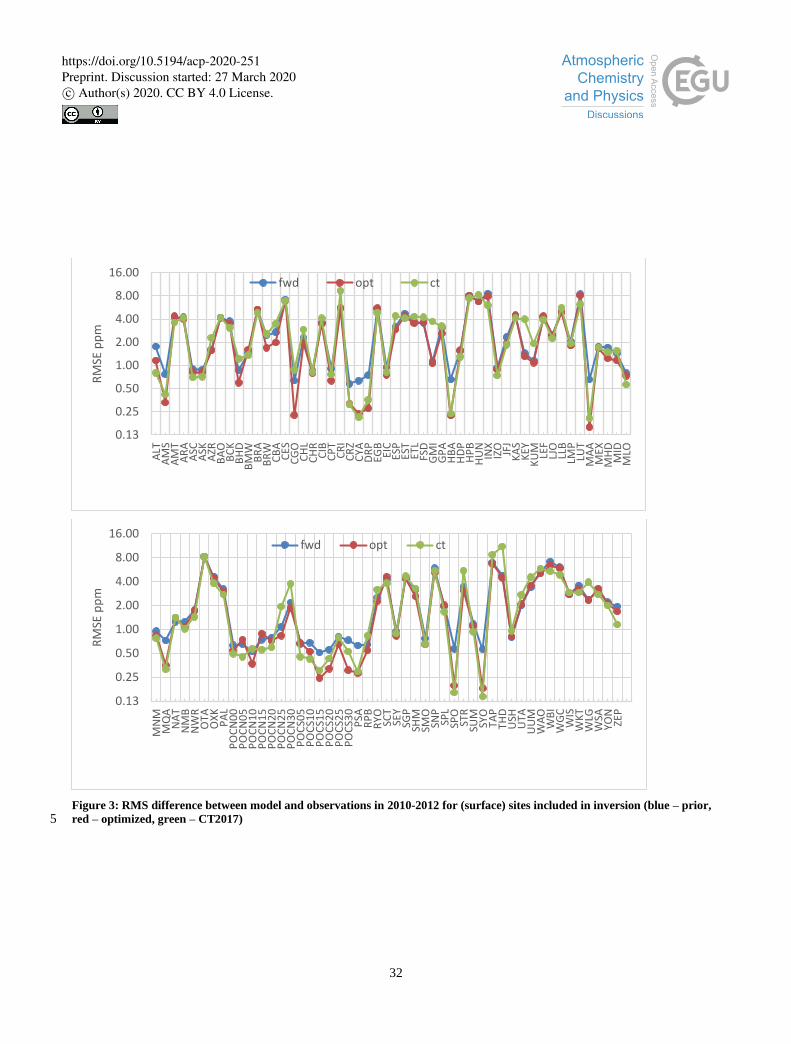
32

Figure 3: RMS difference between model and observations in 2010-2012 for (surface) sites included in inversion (blue – prior,

red – optimized, green – CT2017) 5

0.13

0.25

0.50

1.00

2.00

4.00

8.00

16.00

ALT

AM

SA

MT

AR

AA

SCA

SKA

ZRB

AO

BC

KB

HD

BM

WB

RA

BR

WC

BA

CES

CG

OC

HL

CH

RC

IBC

PT

CR

IC

RZ

CYA

DR

PEG

BEI

CES

PES

TET

LFS

DG

MI

GP

AH

BA

HD

PH

PB

HU

NIN

XIZ

O JFJ

KA

SK

EYK

UM

LEF

LJO

LLB

LMP

LUT

MA

AM

EXM

HD

MID

MLO

RM

SE p

pm

fwd opt ct

0.13

0.25

0.50

1.00

2.00

4.00

8.00

16.00

MN

MM

QA

NA

TN

MB

NW

RO

TAO

XK

PA

LP

OC

N0

0P

OC

N0

5P

OC

N1

0P

OC

N1

5P

OC

N2

0P

OC

N2

5P

OC

N3

0P

OC

S05

PO

CS1

0P

OC

S15

PO

CS2

0P

OC

S25

PO

CS3

0P

SAR

PB

RYO SC

TSE

YSG

PSH

MSM

OSN

PSP

LSP

OST

RSU

MSY

OTA

PTH

DU

SHU

TAU

UM

WA

OW

BI

WG

CW

ISW

KT

WLG

WSA

YON

ZEP

RM

SE p

pm

fwd opt ct


33

Figure 4: RMS difference between model and observations in 2010-2012 for aircraft sites, not included in inversion (blue –

prior, red – optimized, green – CT2017)

5

0.25

0.50

1.00

2.00

4.00

8.00

ACG005

ACG015

ACG025

ACG035

ACG045

ACG055

ACG065

ACG075

ACG085

CAR015

CAR025

CAR035

CAR045

CAR055

CAR065

CAR075

CAR085

CMA005

CMA015

CMA025

CMA035

CMA045

CMA055

CMA065

CMA075

CMA085

CONN00

CONN05

CONN10

CONN15

CONN20

CONN25

CONN30

CONS05

CONS15

CONS20

CONS25

CONS30

DND005

DND015

DND025

DND035

DND045

DND055

DND065

DND075

ESP005

ESP015

ESP025

ESP035

ESP045

ESP055

ETL005

ETL015

ETL025

ETL035

ETL045

ETL055

ETL065

ETL075

HIL005

HIL015

HIL025

HIL035

HIL045

HIL055

HIL065

HIL075

HIL085

INX005

RM

SE p

pm

fwd opt opt-ct

0.25

0.50

1.00

2.00

4.00

8.00

INX015

INX025

INX035

LEF005

LEF015

LEF025

LEF035

NHA005

NHA015

NHA025

NHA035

NHA045

NHA055

NHA065

NHA075

PFA

005

PFA

015

PFA

025

PFA

035

PFA

045

PFA

055

PFA

065

PFA

075

RTA

005

RTA

015

RTA

025

RTA

035

RTA

045

RTA

055

RTA

065

SCA005

SCA015

SCA025

SCA035

SCA045

SCA055

SCA065

SCA075

SCA085

SGP005

SGP015

SGP025

SGP035

SGP045

SGP055

TGC005

TGC015

TGC025

TGC035

TGC045

TGC055

TGC065

TGC075

TGC085

THD005

THD015

THD025

THD035

THD045

THD055

THD065

THD075

WBI005

WBI015

WBI025

WBI035

WBI045

WBI055

WBI065

WBI075

WBI085

RM

SE p

pm

fwd opt opt-ct


Documents

Technical note: A h igh -resolution inverse modelling