GIStechnical

30 PositionIT -Aug/Sept 2009

Landform classification using GIS

by Karsten Drescher, Terralogix Consulting, and Willem de Frey, Ekoinfo

Refining existing landform classifications using ESRI’s model builder.

Landforms form an integral part of the landscape; they reflect the influence of geology and

climate [1] on a regional/broad scale. The combination of landform and climate influences the development of soil conditions, which influence the distribution and extent of certain plant communities and associated animal assemblages [2]. The significance of landforms in terms of understanding the potential and constraints within the landscape associated with them, is well documented [3]. Gauteng Province Department of Agriculture, Conservation and Environment Directorate Nature Conservation’s Ridges Policy [4] support this statement.

On a large/fine scale the different facets/units associated with landforms such as crests, scarps, midslopes, footslopes and valley bottoms present habitat for flora and fauna. The more complex the morphology of the landform is, the higher its potential to support a variety of organisms at a variety of densities [5]. Thus knowing the extent and distribution of landforms, whether complex such as ridges, tablelands, hills and mountains or simple such as highly productive plains and valleys [6], is very important in terms of environmental management to assess the conservation significance and potential of a portion of land within the landscape to be developed or affected by human activities.

From a geological and engineering geological perspective, landforms are of specific interest as the landforms were created by geological processes. The existing landforms also play a significant role in the current sedimentary processes.

Existing data

Existing morphology maps [7, 8], which are part of the environmental

potential atlas, are based on the work done by Kruger [9] in 1983 (Fig. 1) and give the classification of the morphological divisions in

South Africa (see Fig. 2 ) as well as the finer detailed morphological units on a provincial scale. Looking at the map for Gauteng (Fig. 3), the

Fig. 1: Terrain morphology map of Southern Africa (after Kruger [9]).

Fig. 2: Terrain morphological divisions of South Africa (after Breedlove and Fraser [7, 8]).

technicalGIS

PositionIT -Aug/Sept 2009 31

classifications are still fairly broad. Kruger’s map was done at a scale of 1:8 000 000.

The Department of Agriculture, Conservation and the Environment of the Gauteng Provincial Government has a policy on ridges [4] which is based on the slope values derived from a digital terrain model (DTM) (Fig. 4).

Fig. 3: Terrain morphological units of Gauteng (after Breedlove and Fraser [7, 8]).

Fig. 4: Ridges as defined by GDACE (after Pfab [4]).

Apart for classifying landforms with more detail, the need was also identified to define ridges using more parameters than just the slope values.

Methodology and results

The landscape classification was done similar to that done by Morgan and Lesh [10].

Two landform classifications were done. The first one was done for the Gauteng province using a digital terrain model (DTM) with a pixel size of 30 m, derived from contour lines with a height interval of 20 m.

The second one for South Africa was done using a DTM with a 200 m pixel resolution, based on contour lines with an interval of 100 m.

The calculations were done using ESRI’s modelbuilder (ArcGIS 9.3 with 3D Analyst and Spatial Analyst extensions).

For Gauteng, the GIS process that was followed is described in detail by Morgan and Lesh [10]. The most recent available boundary of Gauteng as defined by the Municipal Demarcation Board [11] was used and projected to Lo 84/29 (WG29), and a buffer of 5 km was added. Although some of the boundary effects are taken care of mathematically, any remaining edge effects are minimised using a 5 km buffer. A rectangle covering the study area (Gauteng plus buffer) was determined. Contour lines with a 20 m interval were merged and the dataset was projected to the Lo 84/29 (WG29) projection and clipped with the above mentioned rectangle. It was discovered that the dataset is too large for a straight “Topo to Raster” (3D Analyst) process. A TIN dataset was created using this clipped contour dataset. The TIN dataset was then converted to an elevation raster dataset with a 30 m pixel resolution.

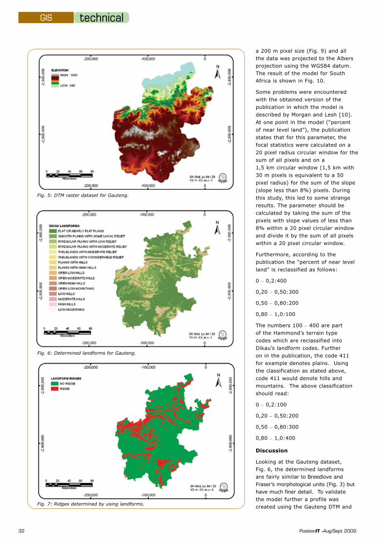
The Gauteng-plus-buffer feature was converted to a raster dataset such that pixels inside the polygon are assigned a value of one (1) and the pixels outside the polygon are assigned “No data”. Multiplying this raster with the elevation raster resulted in a DTM raster (see Fig. 5). As the “No data” pixels are ignored during the processing it speeds up the processing which consists of 37 calculation steps. As far as computing time is concerned the model builder runs the model within 3 hours on a 2,4 GHz quad processor PC with 2 GB RAM. The resulting Dikau [7] landforms are shown on Fig. 6.

The results for the Gauteng dataset were analysed further by comparing it to the GDACE ridge dataset. For this purpose the determined landforms “Flat or nearly flat plains” and “Smooth plains with some local relief” were classified as “No ridges” while all the other landforms were classified as “Ridges” as shown on Fig. 7. The result of the comparative study is shown on Fig. 8.

For South Africa the above-mentioned process was repeated with a DTM with

technicalGIS

32 PositionIT -Aug/Sept 2009

Fig. 5: DTM raster dataset for Gauteng.

Fig. 6: Determined landforms for Gauteng.

Fig. 7: Ridges determined by using landforms.

a 200 m pixel size (Fig. 9) and all the data was projected to the Albers projection using the WGS84 datum. The result of the model for South Africa is shown in Fig. 10.

Some problems were encountered with the obtained version of the publication in which the model is described by Morgan and Lesh [10]. At one point in the model (“percent of near level land”), the publication states that for this parameter, the focal statistics were calculated on a 20 pixel radius circular window for the sum of all pixels and on a 1,5 km circular window (1,5 km with 30 m pixels is equivalent to a 50 pixel radius) for the sum of the slope (slope less than 8%) pixels. During this study, this led to some strange results. The parameter should be calculated by taking the sum of the pixels with slope values of less than 8% within a 20 pixel circular window and divide it by the sum of all pixels within a 20 pixel circular window.

Furthermore, according to the publication the “percent of near level land” is reclassified as follows:

0 – 0,2:400

0,20 – 0,50:300

0,50 – 0,80:200

0,80 – 1,0:100

The numbers 100 – 400 are part of the Hammond’s terrain type codes which are reclassified into Dikau’s landform codes. Further on in the publication, the code 411 for example denotes plains. Using the classification as stated above, code 411 would denote hills and mountains. The above classification should read:

0 – 0,2:100

0,20 – 0,50:200

0,50 – 0,80:300

0,80 – 1,0:400

Discussion

Looking at the Gauteng dataset, Fig. 6, the determined landforms are fairly similar to Breedlove and Fraser’s morphological units (Fig. 3) but have much finer detail. To validate the model further a profile was created using the Gauteng DTM and

technicalGIS

PositionIT -Aug/Sept 2009 33

Fig. 8: Comparison between GDACE ridges and landform ridges.

Fig. 9: DTM for South Africa.

Fig. 10: Determined landforms for South Africa.

superimposed onto the landform classification as shown in Fig. 11. Furthermore, using the determined landforms to define ridges compares very well to GDACE’s ridge dataset (Fig. 7).

For the South African dataset, Fig. 10, the determined landforms compare fairly well to Breedlove and Fraser’s morphological divisions (Fig. 2), but have much finer detail.

Comparing the landform classification of Gauteng to the one for South Africa (Fig. 6 and Fig. 10), there is similarity between them but not an exact match. This is to be expected as the model uses an elevation range from 940 to 1900 m above sea level for the Gauteng dataset and an elevation range of sea level to 3700 m above sea level for the South African dataset. Furthermore the focal statistics are determined over the same number of pixels (20 pixel circular window) but the pixels size of the South African dataset is 200 m compared to the Gauteng dataset where the pixel size is 30 m.

Conclusions

The above mentioned results show that the model appears to produce acceptable results. It is however important to note that the determined landforms are not necessarily absolute but relative to the dataset. This is more prevalent on the mountainous terrains: a plain on the Gauteng dataset is also a plain on the national dataset but a landform that is a high hill compared to the rest of Gauteng is not necessarily a high hill when compared to the rest of South Africa.

A further conclusion made is that the ridges determined by the landforms is mainly in agreement with the GDACE ridge policy based on slopes – the ridges policy can however be somewhat refined.

References

[1] A N Strahler, & A H Strahler: Modern

Physical Geography Third Edition.

Wiley and Sons, New York, 1987.

[2] M G Barbour, J H Burk and W D Pitts:

Terrestrial Plant Ecology. Benjamin/

Cummings Publishing Company,

California, 1980.

[3] J A Wiens, M R Moss, M G Turner and

Geospace

¼

? Irene size

technicalGIS

34 PositionIT -Aug/Sept 2009

Fig. 11: Profile (vertically exaggerated) through the Gauteng DTM.

D J Mladenoff: Foundation Papers in Landscape Ecology. Columbia University Press, New York, 2006.

[4] M Pfab: Development Guidelines

for Ridges. Departmental Policy.

Department of Agriculture, Conservation,

Environment and Land Affairs Directorate

of Nature Conservation, 2001.

[5] M G Turner, R H Gardner and R V O'Neill:

Landscape Ecology in Theory and

Practice Pattern and Process, Springer,

USA, 2001.

[6] D B Lindenmayer and J Fischer: Habitat

Fragmentation and Landscape Change

An Ecological And Conservation

Synthesis, Island Press, USA, 2006.

[7] G Breedlove and F Fraser: Environmental

Potential Atlas for South Africa: Terrain

Morphological Divisions, online at

www.environment.gov.za/Enviro-Info/

nat/images/mdiv.jpg, Department of

Environmental Affairs and Tourism,

University of Pretoria & GIS Business

Solutions, 2000.

[8] G Breedlove and F Fraser: Environmental

Potential Atlas for Gauteng: Terrain

Morphological Units, online at

www.environment.gov.za/Enviro-Info/

prov/gt/gtmorp.jpg, Department of

Environmental Affairs and Tourism,

University of Pretoria and GIS Business

Solutions, 2000.

[9] G P Kruger: Terrain morphology map

of Southern Africa, Soil and Irrigation

Research Institute, Department of

Agriculture, Pretoria, 1983.

[10] J M Morgan and A M Lesh: Developing

Landform Maps Using ESRI's

Modelbuilder, online at

http://gis.esri.com/library/userconf/

proc05/papers/pap2206.pdf, 2005.

[11] Municipal Demarcation Board.

RSA_Prov.zip, online

www.demarcation.org.za/, 2007.

Contact Karsten Drescher, Terralogix Consulting, 012 803-8735, terralogix@telkomsa.net

Advertorial

Missing a file in the field? No problem with Trimble Access