TECHNICAL ISO/TR REPORT 230-8allaboutmetallurgy.com/wp/wp-content/uploads/2016/12/… · · 2017-01-301) In some cases, practical considerations require that real or dummy tooling

Reference numberISO/TR 230-8:2009(E)

© ISO 2009

TECHNICAL REPORT

ISO/TR230-8

First edition2009-01-15

Test code for machine tools — Part 8: Determination of vibration levels

Code d'essai des machines-outils —

Partie 8: Détermination des niveaux de vibration

Copyright International Organization for Standardization Provided by IHS under license with ISO

Not for ResaleNo reproduction or networking permitted without license from IHS

--`,,```,,,,````-`-`,,`,,`,`,,`---

ISO/TR 230-8:2009(E)

PDF disclaimer This PDF file may contain embedded typefaces. In accordance with Adobe's licensing policy, this file may be printed or viewed but shall not be edited unless the typefaces which are embedded are licensed to and installed on the computer performing the editing. In downloading this file, parties accept therein the responsibility of not infringing Adobe's licensing policy. The ISO Central Secretariat accepts no liability in this area.

Adobe is a trademark of Adobe Systems Incorporated.

Details of the software products used to create this PDF file can be found in the General Info relative to the file; the PDF-creation parameters were optimized for printing. Every care has been taken to ensure that the file is suitable for use by ISO member bodies. In the unlikely event that a problem relating to it is found, please inform the Central Secretariat at the address given below.

COPYRIGHT PROTECTED DOCUMENT © ISO 2009 All rights reserved. Unless otherwise specified, no part of this publication may be reproduced or utilized in any form or by any means, electronic or mechanical, including photocopying and microfilm, without permission in writing from either ISO at the address below or ISO's member body in the country of the requester.

ISO copyright office Case postale 56 • CH-1211 Geneva 20 Tel. + 41 22 749 01 11 Fax + 41 22 749 09 47 E-mail [email protected] Web www.iso.org

Published in Switzerland

ii © ISO 2009 – All rights reserved



--`,,```,,,,````-`-`,,`,,`,`,,`---

ISO/TR 230-8:2009(E)

© ISO 2009 – All rights reserved iii

Contents Page

Foreword............................................................................................................................................................. v Introduction ....................................................................................................................................................... vi 1 Scope ..................................................................................................................................................... 1 2 Normative references ........................................................................................................................... 1 3 Terms and definitions........................................................................................................................... 2 4 Theoretical background to the dynamic behaviour of machine tools .......................................... 13 4.1 Nature of vibration: basic concepts.................................................................................................. 13 4.2 Single-degree-of-freedom systems................................................................................................... 16 4.3 Mathematical considerations ............................................................................................................ 20 4.4 Graphical representations ................................................................................................................. 22 4.5 Different types of harmonic excitation and response..................................................................... 26 4.6 More degrees of freedom................................................................................................................... 33 4.7 Other miscellaneous types of excitation and response of machine tools ................................... 40 4.8 Spectra, responses and bandwidth .................................................................................................. 43 5 Types of vibration and their causes ................................................................................................. 44 5.1 Vibrations occurring as a result of unbalance ................................................................................ 44 5.2 Vibrations occurring through the operation of linear slides.......................................................... 48 5.3 Vibrations occurring externally to the machine .............................................................................. 49 5.4 Vibrations initiated by the machining process: forced vibration and chatter.............................. 50 5.5 Other sources of excitation ............................................................................................................... 52 6 Practical testing: general concepts .................................................................................................. 54 6.1 General................................................................................................................................................. 54 6.2 Measurement of vibration values...................................................................................................... 54 6.3 Instrumentation................................................................................................................................... 55 6.4 Relative and absolute measurements .............................................................................................. 56 6.5 Units and parameters ......................................................................................................................... 56 6.6 Uncertainty of measurement ............................................................................................................. 58 6.7 Note on environmental vibration evaluation.................................................................................... 58 6.8 Type testing......................................................................................................................................... 59 6.9 Location of machine ........................................................................................................................... 59 7 Practical testing: specific applications ............................................................................................ 60 7.1 Unbalance............................................................................................................................................ 60 7.2 Machine slide acceleration along its axis (inertial cross-talk) ....................................................... 64 7.3 Vibrations occurring externally to the machine .............................................................................. 67 7.4 Vibrations occurring through metal cutting .................................................................................... 67 8 Practical testing: structural analysis through artificial excitation ................................................ 68 8.1 General................................................................................................................................................. 68 8.2 Spectrum analysis and frequency response testing ...................................................................... 69 8.3 Machine set-up conditions ................................................................................................................ 70 8.4 Frequency analysis............................................................................................................................. 71 8.5 Modal analysis .................................................................................................................................... 72 8.6 Cross-response tests ......................................................................................................................... 73 8.7 “Non-standard” vibration modes ...................................................................................................... 74 8.8 Providing standard stability tests ..................................................................................................... 75 Annex A (informative) Overview and structure of this part of ISO 230....................................................... 76 Annex B (informative) Relationships between vibration parameters ......................................................... 77



--`,,```,,,,````-`-`,,`,,`,`,,`---

ISO/TR 230-8:2009(E)

iv © ISO 2009 – All rights reserved

Annex C (informative) Summary of basic vibration theory .......................................................................... 79 Annex D (informative) Spindle and motor balancing protocol .................................................................... 83 Annex E (informative) Examples of test results and their presentation ..................................................... 84 Bibliography ..................................................................................................................................................... 93



--`,,```,,,,````-`-`,,`,,`,`,,`---

ISO/TR 230-8:2009(E)

© ISO 2009 – All rights reserved v

Foreword

ISO (the International Organization for Standardization) is a worldwide federation of national standards bodies (ISO member bodies). The work of preparing International Standards is normally carried out through ISO technical committees. Each member body interested in a subject for which a technical committee has been established has the right to be represented on that committee. International organizations, governmental and non-governmental, in liaison with ISO, also take part in the work. ISO collaborates closely with the International Electrotechnical Commission (IEC) on all matters of electrotechnical standardization.

International Standards are drafted in accordance with the rules given in the ISO/IEC Directives, Part 2.

The main task of technical committees is to prepare International Standards. Draft International Standards adopted by the technical committees are circulated to the member bodies for voting. Publication as an International Standard requires approval by at least 75 % of the member bodies casting a vote.

In exceptional circumstances, when a technical committee has collected data of a different kind from that which is normally published as an International Standard (“state of the art”, for example), it may decide by a simple majority vote of its participating members to publish a Technical Report. A Technical Report is entirely informative in nature and does not have to be reviewed until the data it provides are considered to be no longer valid or useful.

Attention is drawn to the possibility that some of the elements of this document may be the subject of patent rights. ISO shall not be held responsible for identifying any or all such patent rights.

ISO/TR 230-8 was prepared by Technical Committee ISO/TC 39, Machine tools, Subcommittee SC 2, Test conditions for metal cutting machine tools.

ISO/TR 230 consists of the following parts, under the general title Test code for machine tools :

⎯ Part 1: Geometric accuracy of machines operating under no-load or finishing conditions

⎯ Part 2: Determination of accuracy and repeatability of positioning numerically controlled axes

⎯ Part 3: Determination of thermal effects

⎯ Part 4: Circular tests for numerically controlled machine tools

⎯ Part 5: Determination of the noise emission

⎯ Part 6: Determination of positioning accuracy on body and face diagonals (Diagonal displacement tests)

⎯ Part 7: Geometric accuracy of axes of rotation

⎯ Part 8: Determination of vibration levels [Technical Report]

⎯ Part 9: Estimation of measurement uncertainty for machine tool tests according to series ISO 230, basic equations [Technical Report]



--`,,```,,,,````-`-`,,`,,`,`,,`---

ISO/TR 230-8:2009(E)

vi © ISO 2009 – All rights reserved

Introduction

The purpose of ISO 230 is to standardize methods of testing the performance of machine tools, generally without their tooling1), and excluding portable power tools. This part of ISO 230 establishes general procedures for the assessment of machine tool vibration.

The need for vibration control is recognized in order that those types of vibration that produce undesirable effects can be mitigated. These effects are identified principally as:

⎯ unacceptable cutting performance with regard to surface finish and accuracy;

⎯ premature wear or damage of machine components;

⎯ reduced tool life;

⎯ unacceptable noise level;

⎯ physiological harm to operators.

Of these, only the first is considered to lie within the scope of this part of ISO 230, although the other effects may well occur incidentally. (Noise is covered by ISO 230-5, and the effect of vibration on operators is covered by ISO 2631-1.) For the most part, this necessarily limits this part of ISO 230 to the problems of vibrations that are generated between tool and workpiece.

Although this part of ISO 230 is in the form of a Technical Report, a number of acceptance tests are proposed within it. These take on the appearance of “standard tests” to be found in other parts of the 230 series. These tests may be used in this way, but, being less rigorous in their formulation, they do not carry the authority that a test in accordance with an International Standard would have.

1) In some cases, practical considerations require that real or dummy tooling and workpieces be used (see 7.1.1, 7.2.1, 7.4 and 8.3).



--`,,```,,,,````-`-`,,`,,`,`,,`---

TECHNICAL REPORT ISO/TR 230-8:2009(E)

© ISO 2009 – All rights reserved 1

Test code for machine tools —

Part 8: Determination of vibration levels

1 Scope

This part of ISO 230 is concerned with the different types of vibration that can occur between the tool-holding part and the workpiece-holding part of a machine tool. (For simplicity, these will generally be referred to as “tool” and “workpiece”, respectively.) These are vibrations that can adversely influence the production of both an acceptable surface finish and an accurate workpiece.

It is not aimed primarily at those who have expertise in vibration analysis and who routinely carry out such work in research and development environments. It does not, therefore, replace standard textbooks on the subject (see the Bibliography). It is, however, intended for manufacturers and users alike with general engineering knowledge in order to enhance their understanding of the causes of vibration by providing an overview of the relevant background theory.

It also provides basic measurement procedures for evaluating certain types of vibration problems that can beset a machine tool:

⎯ vibrations occurring as a result of mechanical unbalance;

⎯ vibrations generated by the operation of the machine’s linear slides;

⎯ vibrations transmitted to the machine by external forces;

⎯ vibrations generated by the cutting process including self-excited vibrations (chatter).

Additionally, this report discusses the application of artificial vibration excitation for the purpose of structural analysis. For further information on how to use this part of ISO 230, see Annex A.

NOTE Other sources of vibration (e.g. the instability of drive systems, the use of ancillary equipment or the effects of worn bearings) are discussed briefly, but a detailed analysis of their vibration generating mechanisms is not given.

2 Normative references

The following referenced documents are indispensable for the application of this document. For dated references, only the edition cited applies. For undated references, the latest edition of the referenced document (including any amendments) applies.

ISO 230-1, Test code for machine tools — Geometric accuracy of machines operating under no-load or finishing conditions

ISO 230-5, Test code for machine tools — Determination of the noise emission

ISO 1925:2001, Mechanical vibration — Balancing — Vocabulary



--`,,```,,,,````-`-`,,`,,`,`,,`---

ISO/TR 230-8:2009(E)

2 © ISO 2009 – All rights reserved

ISO 1940-1:2003, Mechanical vibration — Balance quality requirements for rotors in a constant (rigid) state — Part 1: Specification and verification of balance tolerances

ISO 2041:1990, Vibration and shock — Vocabulary

ISO 2631-1, Mechanical vibration and shock — Evaluation of human exposure to whole-body vibration — Part 1: General requirements

ISO 2954, Mechanical vibration of rotating and reciprocating machinery — Requirements for instruments for measuring vibration severity

ISO 5348:1998, Mechanical vibration and shock — Mechanical mounting of accelerometers

ISO 6103, Bonded abrasive products — Permissible unbalances of grinding wheels as delivered — Static testing

ISO 15641, Milling cutters for high speed machining — Safety requirements

3 Terms and definitions

For the purposes of this document, the terms and definitions given in ISO 1925, ISO 2041 and the following apply.

3.1 absolute vibration vibration value measured with an inertial transducer at a single point

3.2 absorber damper device for reducing the magnitude of a shock or vibration by energy dissipation methods

[ISO 2041:1990, definition 2.114]

3.3 accelerance vibration quantified by its acceleration per unit excitation force

NOTE See Table 1 in ISO 2041.

3.4 aliasing error erroneous result in digital analysis of signals caused by having the maximum frequency of the [measured] signal greater than one-half the value of the sampling frequency

[ISO 2041:1990, definition 5.8]

3.5 amount of unbalance product of the unbalance mass and the distance of its centre of mass from the shaft axis


NOTE This is sometimes referred to as the “residual unbalance” (e.g. in ISO 1940-1). It is measured in mass-length units, e.g. gram millimetres (g·mm).

3.6 amplitude peak vibration value maximum value of a sinusoidal vibration




--`,,```,,,,````-`-`,,`,,`,`,,`---

ISO/TR 230-8:2009(E)


NOTE This is sometimes called vector amplitude to distinguish it from other senses of the term “amplitude”, and it is sometimes called single amplitude, or peak amplitude, to distinguish it from double amplitude, which, for a simple harmonic vibration, is the same as the total excursion or peak-to-peak value. The use of the terms “double amplitude” and “single amplitude” is deprecated.

3.7 angular frequency circular frequency product of the frequency of a sinusoidal quantity and the factor 2π


NOTE 1 The unit of circular frequency is the radian per unit of time.

NOTE 2 Angular or circular frequency occurs at the rate at which any vibration signal (or part of a vibration signal) repeats its pattern. It is measured in radians/s and is usually represented by the symbol “ω ”.

3.8 antinode point, line or surface in a standing wave where some characteristic of the wave field has a maximum value


EXAMPLE A point or line on the surface of a machine tool whose amplitude of vibration (at a particular frequency) is greater than that at any adjacent points or lines.

3.9 antiresonance system in forced oscillation in which any change at a given point, however small, in the frequency of excitation causes an increase in a response at this point

NOTE 1 The above specification defines a response minimum, but not necessarily a response zero.

NOTE 2 Adapted from ISO 2041:1990, definition 2.74.

3.10 averaging process chosen to determine a single representative value for a set of data

NOTE In connection with sine wave analysis, averaging refers to the arithmetic mean signal level in one half of a sine wave and is defined in Annex B. In connection with data sampling, various techniques are available. Vector averaging, for example, not only takes the mean of the signal level but also takes account of its phase relative to some reference frequency (e.g. the excitation frequency). This technique ensures that any signal content that is unrelated to the frequency of interest, and consequently of an undetermined phase for each sample, is rapidly diminished through cancelling as the averaging takes place. This effective enhancer of signal-to-noise ratio also provides a useful diagnostic tool for identifying vibration sources.

3.11 bandwidth range of frequencies (usually expressed in hertz) where the amplitude exceeds a particular threshold level, or limits within which the power spectrum is considered

NOTE This should not be confused with the same term used in digital communication theory for expressing a data transmission rate in bits/s.

3.12 beats periodic variations in the amplitude of an oscillation resulting from the combination of two oscillations of slightly different frequencies

NOTE 1 The beats occur at the difference frequency.




--`,,```,,,,````-`-`,,`,,`,`,,`---

ISO/TR 230-8:2009(E)


3.13 broadband measurement measuring process where the total vibration power is integrated over the frequency range of interest

3.14 centre of mass that point associated with a body which has the property that an imaginary particle placed at this point with a mass equal to the mass of a given material system has a first moment with respect to any plane equal to the corresponding first moment of the system

NOTE This term is sometimes referred to as “centre of inertia” and for most practical situations it is synonymous with “centre of gravity”.


3.15 chatter self-excited regenerative relative vibrations between the tool and workpiece during the cutting process, precipitating an unstable machining condition

NOTE See also 5.4.

3.16 coherence function that fraction of the total power in a response signal that is identified with an individual source component

3.17 coupled modes modes of vibration that are not independent but which influence one another because of energy transfer from one to another


3.18 critical damping ⟨single degree-of-freedom system⟩ amount of viscous damping that corresponds to the limiting condition between an oscillatory and a non-oscillatory transient state of free vibration


3.19 cycle complete range of states or values through which a periodic phenomenon or function passes before repeating itself identically


3.20 damping dissipation of energy with time

NOTE Adapted from ISO 2041:1990, definition 2.79.

3.21 damping ratio ⟨system with linear viscous damping⟩ ratio of the actual damping coefficient to the critical damping coefficient

NOTE Adapted from ISO 2041:1990, definition 2.86.



--`,,```,,,,````-`-`,,`,,`,`,,`---

ISO/TR 230-8:2009(E)


3.22 degrees-of-freedom number of degrees of freedom of a mechanical system equal to the minimum number of independent generalized coordinates required to define completely the configuration of the system at any instant of time


3.23 distributed system continuous system system having an infinite number of possible independent configurations


NOTE Machine tools generally fall into this category as the mass as well as the stiffness are not located at individual points but distributed over the whole structure.

3.24 dynamic compliance reciprocal of dynamic stiffness

NOTE This is quite often referred to as “flexibility”. Typical units are µm/N.

3.25 dynamic stiffness ratio of change of force to change of displacement under dynamic conditions

NOTE 1 See also ISO 2041:1990, definition 1.54.

NOTE 2 At low frequencies, the dynamic stiffness approximates to the static stiffness. At high frequencies, the response tends towards zero and the dynamic stiffness tends towards infinity. At intermediate frequencies, where resonances occur, the dynamic stiffness can drop to a very low value. Units of stiffness are expressed in force per displacement, e.g. N/µm.

3.26 dynamic vibration absorber device for reducing vibrations of a primary system over a desired frequency range by the transfer of energy to an auxiliary system in resonance so tuned that the force exerted by the auxiliary system is opposite in phase to the force acting on the primary system

[ISO 2041:1990, definition 2.116]

NOTE Dynamic vibration absorbers may be damped or undamped, but damping is not the primary purpose.

3.27 FFT fast Fourier transform process where the computing times of complex multiplications and additions are greatly reduced


NOTE 1 For more details, see ISO 2041:1990, A.18 to A.22.

NOTE 2 An FFT is a mathematical algorithm enabling vibration-analysis equipment to perform at high speed and thus appear to function in “real time”.

3.28 forced vibration steady-state vibration caused by a steady-state excitation


NOTE 1 Transient vibrations are not considered.

NOTE 2 The vibration (for linear systems) has the same frequencies as the excitation.



--`,,```,,,,````-`-`,,`,,`,`,,`---

ISO/TR 230-8:2009(E)


3.29 foundation structure that supports a mechanical system and that may be fixed in a specified frame or it may undergo a motion that provides excitation for the supported system


3.30 Fourier analysis mathematical procedure for determining the coefficients and phase angles of the components of the Fourier series for a given waveform

3.31 Fourier series series which expresses the values of a periodic function in terms of discrete frequency components that are harmonically related to each other

[ISO 2041:1990, definition A.18]

NOTE See the notes to the reference in ISO 2041:1990, A.18, for a mathematical description.

3.32 free vibration vibration that occurs after the removal of excitation or restraint


NOTE The system vibrates at natural frequencies of the system.

3.33 frequency reciprocal of the fundamental period, being the smallest increment of the independent variable of a periodic quantity [time] for which the function repeats itself

NOTE 1 Adapted from ISO 2041:1990, definitions 2.23 and 2.24.

NOTE 2 The frequency is the rate at which any vibration signal (or part of a vibration signal) repeats its pattern and is measured in hertz (Hz), which is the number of cycles per second.

3.34 frequency response output signal expressed as a function of the frequency of the input signal

NOTE 1 On a machine tool the frequency response is often limited to the expression of the ratio of the relative displacement between tool and workpiece (output signal) to the excitation force (input signal). See also 4.3 et seq. The magnitude of the frequency response is equivalent to the dynamic compliance. The frequency response is, however, a complex quantity and requires two numbers to define it fully: either “magnitude” and “phase”, or “real part” and “imaginary part”. In some texts the term “receptance” is used synonymously with “response”.

NOTE 2 The frequency response is usually given graphically by curves showing the relationship of the output signal and, where applicable, phase shift or phase angle as a function of frequency.

NOTE 3 Adapted from ISO 2041:1990, definition B.13.

3.35 fundamental frequency ⟨periodic quantity⟩ reciprocal of the fundamental period




--`,,```,,,,````-`-`,,`,,`,`,,`---

ISO/TR 230-8:2009(E)


3.36 harmonic ⟨periodic quantity⟩ sinusoid, the frequency of which is an integral multiple of the fundamental frequency


NOTE 1 The term “overtone” has frequently been used in place of “harmonic”, the nth harmonic being called the (n-1)th overtone.

NOTE 2 In English, the first overtone and the second harmonic are each twice the frequency of the fundamental. In French, the distinction between harmonic and overtone does not exist, and the second harmonic is twice the frequency of the fundamental. The term “overtone” is now deprecated to reduce ambiguity in the numbering of the components of a periodic quantity.

3.37 harmonic distortion ⟨periodic wave⟩ amount of vibrational energy existing at second and subsequent harmonic frequencies compared with the total vibrational energy present

3.38 imaginary part that part of the displacement frequency response that is in quadrature (90° out-of-phase) with the excitation

NOTE For a simple vibration system, the imaginary part reaches a maximum at the undamped natural frequency.

3.39 impulse integral with respect to time of a force taken over the time during which the force is applied, which, for a constant force, is the product of the force and the time during which the force is applied


NOTE The “impulsive” force may act over a very short time and change rapidly during the event, often reaching a very high instantaneous value. Typical examples are a hammer blow or a rapidly accelerating machine slide. Impulses are measured in units of force multiplied by time, e.g. N·s.

3.40 inertial cross-talk displacements perpendicular to the intended direction of motion owing to a lateral offset between the driving force and the centre of mass, which lead to tilt motions during acceleration and deceleration

3.41 instrumented hammer hammer incorporating a force transducer that is capable of transmitting a broadband frequency response of the impact delivered by the hammer when used to strike a structure

3.42 linear system system in which the response is proportional to the magnitude of the excitation


3.43 mass eccentricity distance between the centre of mass of a rigid rotor and the shaft axis




--`,,```,,,,````-`-`,,`,,`,`,,`---

ISO/TR 230-8:2009(E)


3.44 mobility complex ratio of the velocity, taken at a point in a mechanical system, to the force taken at the same or another point in the system, during simple harmonic motion


3.45 modal mass equivalent mass in a single degree-of-freedom system for a particular mode

3.46 mode of vibration ⟨system undergoing vibration⟩ mode of vibration designates the characteristic pattern of nodes and antinodes assumed by the system in which the motion of every particle, for a particular frequency, is simple harmonic (for linear systems) or has corresponding decay patterns


NOTE In a machine tool, individual modes of vibration are characterized by the different relative movements of the basic structural elements. For a particular frequency at any point in time, the instantaneous disposition of these elements will determine the characteristic modal shape for that frequency.

3.47 modulation, amplitude and frequency periodic wave whose amplitude and/or frequency is itself varying as a result of an imposed signal. Modulated signals are characterized by the presence of side-band frequencies

3.48 multi-degree-of-freedom system system for which two or more co-ordinates are required to define completely the configuration of the system at any instant


3.49 narrow-band measurement measuring process where the vibration power over a specified narrow bandwidth of frequencies is measured

3.50 natural frequency frequency of the free vibration of a damped linear system


EXAMPLE The frequency at which a structure will vibrate freely when all forced vibration is removed, which in practice is the damped natural frequency. (The undamped natural frequency occurs when the phase shift is 90°.)

3.51 node point, line or surface in a standing wave where some characteristic of the wave field has essentially zero amplitude

EXAMPLE A point or line of little or minimal movement between two parts of the machine, which, at any given instant, are moving in opposite directions.




--`,,```,,,,````-`-`,,`,,`,`,,`---

ISO/TR 230-8:2009(E)


3.52 non-linearity property of a system in which the response is specifically not proportional to the magnitude of the excitation.

NOTE Systems with non-linear stiffness are usually identified either as “stiffening” or “softening”.

3.53 oscillation variation, usually with time, of the magnitude of a quantity with respect to a specified reference when the magnitude is alternately greater and smaller than some mean value


3.54 peak-to-peak vibration value algebraic difference between the extreme values of the vibration


EXAMPLE The total “displacement” movement of the vibration.

NOTE This is twice the amplitude and is sometimes also referred to as “double amplitude”. This term is non-preferred and loses its relevance for velocity and acceleration vibration signals.

3.55 period fundamental period smallest increment of the independent variable of a periodic quantity for which the function repeats itself


3.56 periodic force periodic motion periodic quantity, the values of which recur for certain equal increments of the independent variable (time)


EXAMPLE Exciting force or motion that repeats its wave pattern at a regular rate.

NOTE The waveform is not necessarily sinusoidal; the force or motion is characterized by its frequency components.

3.57 phase phase angle fractional part of a period through which a sinusoidal vibration has advanced as measured from a value of the independent variable as a reference


EXAMPLE The angular delay between two otherwise similar vibration signals.

NOTE This delay is either measured in degrees in terms of the vibration period (which is counted as 360°) or in radians. Thus, two vibrations moving in opposite directions to each other at the same instant are 180° or π radians out of phase.

3.58 power spectrum spectrum of mean-squared spectral density values




--`,,```,,,,````-`-`,,`,,`,`,,`---

ISO/TR 230-8:2009(E)


3.59 Q Q factor quantity which is a measure of the sharpness of resonance of a resonant oscillatory system having a single degree of freedom

NOTE 1 The Q factor is sometimes referred to as the magnification factor. It is equal to one half of the reciprocal of the damping ratio. See also 4.3.3 and Equation (19).


3.60 real part that part of the displacement frequency response that is in phase with the excitation

NOTE For a simple vibration system, the real part reaches a maximum positive value just before resonance and a maximum negative value just after resonance. At the undamped natural frequency, it is zero. For some types of machine, the size of the maximum negative value provides a measure of the machine’s potential instability at that frequency.

3.61 regenerative vibration vibration that is sustained through resonance and draws its energy through feedback from an ongoing process

EXAMPLE Machine tool chatter.

3.62 relative vibration vibration value measured between two locations (e.g. tool and workpiece) using a suitable transducer attached through a movable member to both locations

3.63 resonance ⟨system in forced oscillation⟩ any change, however small, in the frequency of excitation causing a decrease in a response of the system


NOTE The condition of resonance exists when the frequency of forced vibration is close to the natural frequency (q.v.) of the structure.

3.64 resonance frequency frequency at which resonance exists


NOTE 1 For more information, see 4.3; for extended definitions, see also ISO 2041:1990, 2.73, Notes 2 and 3, and Table 2.

NOTE 2 The term “resonant frequency” is often used as a popular but syntactically imprecise alternative to “resonance frequency”.

3.65 rms value root-mean-square value ⟨single-valued function⟩ square root of the average of the squared values of the function over a (given) interval

[ISO 2041:1990, definition A.37]

NOTE This is a way of mathematically averaging the power of a vibration signal and is often used when the waveform of the signal departs from the sinusoidal waveform. See also Annex B.



--`,,```,,,,````-`-`,,`,,`,`,,`---

ISO/TR 230-8:2009(E)


3.66 sampling obtaining the values of a function for regularly or irregularly spaced distinct values from its domain


3.67 sampling frequency number of samples taken in one second


3.68 sampling interval time interval between two samples


3.69 signal vibration signal disturbance variation of a physical quantity used to convey information

[ISO 2041:1990, definition B.1]

EXAMPLE A varying electrical voltage obtained as an analogue of mechanical vibration by means of a transducer. The voltage can be proportional to the displacement, velocity or acceleration of a mechanical vibration or the instantaneous force level, according to the type of transducer used and any subsequent processing.

3.70 simple harmonic vibration, sinusoidal vibration periodic vibration that is a sinusoidal function of the independent variable


NOTE A periodic vibration consisting of the sum of more than one sinusoid, each having a frequency that is a multiple of the fundamental frequency, is often referred to as a complex vibration or a multi-sinusoidal vibration.

3.71 single-degree-of-freedom system system requiring but one co-ordinate to define completely its configuration at any instant


EXAMPLE An idealized basic vibration system comprising a single mass, spring and damper.

NOTE The representation of such a system is shown in Figure 2 and its response characteristic is shown in Figure 4.

3.72 spectrum description of a quantity as a function of frequency or wavelength


3.73 standing wave periodic wave having a fixed amplitude distribution in space, i.e. the result of interference of progressive waves of the same frequency and kind




--`,,```,,,,````-`-`,,`,,`,`,,`---

ISO/TR 230-8:2009(E)


NOTE 1 A standing wave can be considered to be the result of the superposition of opposing progressive waves of the same frequency and kind.

NOTE 2 Standing waves are characterized by nodes and antinodes that are fixed in position.

3.74 steady-state vibration steady-state vibration exists if the vibration is a continuing periodic vibration


3.75 transducer device designed to receive energy from one system and supply energy, of either the same or of a different kind, to another in such a manner that the desired characteristics of the input energy appear at the output


NOTE A transducer produces an electrical signal analogous to the displacement, velocity or acceleration characteristic of the vibration to be measured.

3.76 transfer function mathematical relation between the output (or response) and the input (or excitation) of the system


NOTE It is usually given as a function of frequency and is usually a complex function.

3.77 transient vibration vibratory motion of a system other than steady-state or random


3.78 transmissibility non-dimensional ratio of the response amplitude of a system in steady-state forced vibration to the excitation amplitude. The ratio may be one of forces, displacements, velocities or accelerations


3.79 unbalance condition that exists in a rotor when vibration force or motion is imparted to its bearings as a result of centrifugal forces


NOTE 1 The geometrical condition of a rotating element occurring when the centre of mass is eccentric to the centre of rotation. This generates a forced vibration proportional to the amount of the unbalance and to the square of the rotational velocity.

NOTE 2 See also ISO 1940-1.

3.80 unbalance mass mass whose centre is at distance from the shaft axis




--`,,```,,,,````-`-`,,`,,`,`,,`---

ISO/TR 230-8:2009(E)


3.81 vibration variation with time of the magnitude of a quantity which is descriptive of the motion or position of a mechanical system, when the magnitude is alternately greater and smaller than some average value or reference


EXAMPLE The periodic relative motion between tool and workpiece caused by a mechanical disturbance. At any instant this motion can be quantified by measurements of displacement, velocity or acceleration. The steady-state magnitude of the vibration can be defined as either the maximum or the rms value of any of these quantities. It can additionally be characterized by its frequency.

NOTE 1 In vibration terminology, the term “level”, i.e. vibration level, may sometimes be used to denote amplitude, average value, rms value, or ratios of these values. These uses are deprecated.

NOTE 2 For the precise use of the term “level” in the logarithmic sense, see ISO 2041:1990, 1.57.

NOTE 3 See also Table A.1.

3.82 viscous damping linear viscous damping dissipation of energy that occurs when an element or part of a vibration system is resisted by a force the magnitude of which is proportional to the velocity of the element and the direction of which is opposite to the direction of the velocity


3.83 waveform characteristic shape of one period of the vibration signal

NOTE A sinusoidal vibration (like a sine wave) is characterized by a single frequency. All other repeating wave patterns contain a mixture of harmonics or integral multiples of the underlying or “fundamental” frequency.

4 Theoretical background to the dynamic behaviour of machine tools

This clause presents the fundamentals of vibration theory relevant to machine tool dynamics. Not intended for the expert, a simplified account is offered where many concepts are explained with only minimal recourse to detailed mathematics. The aim is to equip the practical engineer with sufficient information to be able to understand and evaluate vibration problems, and to carry out the basic tests described in Clauses 7 and 8. Where it is necessary to explore more technically difficult aspects of this subject, including mathematical formulae, the relevant material is presented in a series of separate “Technical Boxes”. These may be safely skipped over by the user requiring simply a general overview. In some cases, it is possible to touch on certain topics only quite briefly. Interested readers should pursue these topics further through the references in the Bibliography.

NOTE A brief summary of the essential content of this clause is presented in Annex C.

4.1 Nature of vibration: basic concepts

Vibration is a physical oscillation of a machine structure brought about by a dynamic excitation force reacting with the machine’s physical properties of mass, stiffness and damping (see 3.81).



--`,,```,,,,````-`-`,,`,,`,`,,`---

ISO/TR 230-8:2009(E)


4.1.1 Displacement, velocity and acceleration of simple harmonic motion (SHM)

At its simplest, the oscillation is in the form of a time-varying sine wave, also known as simple harmonic motion (SHM). The movement is characterized by continuously varying instantaneous values for displacement, velocity and acceleration, each of which follows a sinusoidal waveform — see Figure 1. A harmonic vibration can be evaluated by measuring the maximum root mean square (rms)2), or the instantaneous values of any of these quantities. Unless otherwise specified, a value for displacement, velocity or acceleration is generally taken to mean the maximum value (or amplitude) within a cycle or the static value.

Key PA time delay expressed as phase angle, in degrees Iv instantaneous value of waveforms (arbitrary units) 1 displacement 2 acceleration 3 velocity

Figure 1 — Relative phase angles of displacement, velocity and acceleration for simple harmonic motion

The abscissa of Figure 1 shows the time delay, tdel, in terms of a fraction of the periodic or cycle time, T. It is shown here as a phase angle, in degrees, emphasizing the trigonometric provenance of the wave function, with 360° representing a full cycle or period and the phase angle = 360 × tdel /T. It is important to understand the relative phase and time delay relationships that exist between the waves representing acceleration, velocity and displacement. From the Figure 1 it can be seen that velocity “leads” the displacement by a quarter of a period or 90°, and acceleration leads by a further quarter of a period, that is, with a “phase angle” of 180° with respect to the displacement.

The relative amplitudes of these quantities are mathematically related, but not necessarily as shown in Figure 1 because the relationships depend on the particular vibration frequency.

2) The rms value should not be confused with the mean value, which is essentially zero over a complete cycle.



--`,,```,,,,````-`-`,,`,,`,`,,`---

ISO/TR 230-8:2009(E)


4.1.2 Frequency

Frequency, f, is the reciprocal of the period, T, of the waveform in seconds for one cycle, corresponding to a “phase angle” of 360° in Figure 1. Frequency, expressed in s–1, is measured in hertz (Hz), where 1 Hz = 1 cycle per second, although in many formulae it is more convenient to replace the frequency in Hz by the circular frequency (or “pulsatance”3)) in radians/s. [Note that f is usually used for a frequency in Hz, and ω for a (circular) frequency in rad/s, where f = ω/2π rad/s.] For a constant displacement amplitude, the velocity increases with frequency, and the acceleration increases further with the square of the frequency — see Equations (1), (2) and (3). (See also Annex B for further information on this topic.)

The instantaneous displacement, velocity, and acceleration of SHM are related as follows:

0

0

22

02

displacement sin ... (1)

velocity cos ... (2)

acceleration sin ... (3)

x x tdxx x tdt

d xx x tdt

ω

ω ω

ω ω

= = ×

= = = ×

= = = − ×

where

x0 driving displacement amplitude;

ω circular frequency;

t time.

Technical Box 1 — Formulae for absolute values of displacement, velocity and acceleration for simple harmonic motion

4.1.3 Excitation; transfer functions

Excitation of vibration can either arise kinematically from the essential mechanisms required for the functioning of the machine, or be generated through the cutting process (interaction between tool and workpiece), or else be transmitted through the floor from some external source. And further, for the specific purpose of testing the machine, it can be supplied by an artificial exciter. The various types of vibration source likely to be encountered on a machine tool are discussed in Clause 5, while artificial excitation is covered in Clause 8. In each case, vibration is initiated through an oscillating force, F. However, the waveform of this force will not necessarily conform to the idealized simple harmonic motion described in 4.1.1 and shown in Figure 1. It could take the form of an “impulse”, a “step function” or a complex combination of any of these — and, in a special case, it might even be a non-varying (i.e. “static”) force.

The relationship between the resulting vibration (displacement amplitude, x) and the input force, F, (with respect to frequency) is generally known as a transfer function of the system, and is often denoted by the symbol G, where G = x/F. There can be a number of separate transfer functions determined by which inputs and outputs are being compared.

4.1.4 Energy and momentum

It should be borne in mind that any vibrating mechanical system will have associated with it both energy and momentum, whose universal conservation is enshrined in the basic laws of mechanics.

3) Non-preferred term.



--`,,```,,,,````-`-`,,`,,`,`,,`---

ISO/TR 230-8:2009(E)


“Conservation of momentum” means that a vibrating system always has an equal and opposite momentum to the surface it is sitting on, or the frame it is attached to: it cannot vibrate in isolation. A small mass (e.g. a machine) vibrating with a large displacement amplitude (and hence a high velocity) can sit on a large mass (e.g. a floor) with a small displacement (and hence a small velocity). Nevertheless, the two momenta must always balance: they are always equal and opposite. Remember that momentum is the product of mass times velocity, which, for vibrating systems, is proportional to mass times displacement times frequency.

Conservation of energy has similar implications, though energy can be converted into other forms. During each cycle, kinetic energy (maximum at mid-travel) is continually being transformed to potential energy (maximum at ends of travel) and vice versa. A freely vibrating system that is slowing down through damping (i.e. friction) gradually dissipates its kinetic energy into heat energy (i.e. molecular movement). In the case of forced vibration, the “lost” energy is continuously being replaced and it is therefore more appropriate to consider the power of the vibrating system, i.e. the rate at which energy is being delivered.

4.2 Single-degree-of-freedom systems

The study of machine tool dynamics requires the understanding of some fundamental notions, which can be best illustrated by considering a single-degree-of-freedom system.

4.2.1 The single-degree model

Such a system is shown in Figure 2, and comprises a mass (m) supported by a spring (k) and damper (c). It is called a single-degree system simply because it can vibrate in only one way (i.e. up and down in the figure), and mathematically it has only one independent variable: the displacement (x) of the mass. [The velocity ( )x

and the acceleration ( )x are derivatives of the displacement (see Technical Box 1) and are not therefore independent.]

In Figure 2, an excitation force (see 4.1.3) is shown being applied to this model through the top (i.e. via the mass). The system’s response to this excitation force (F) is the displacement (x) of the mass.

The following properties are assigned to the “idealized” components of this model.

The “massless” spring is resistant only to displacement, x, either in tension or compression, and opposes the applied force by virtue of its stiffness (k). When the spring is at its peak4) displacement downwards (i.e. its maximum compression), it reacts with a force, K = –kx, upwards — see Equation (7). Because the spring displacement is directly proportional to the applied force, this ensures that the model conforms to a linear system.

The mass (m), is resistant only to acceleration and opposes the applied force by virtue of its inertia — Equation (5). Peak acceleration upwards occurs at the bottom of the stroke (see Figure 2), where it reacts with its peak inertia force (M) downwards. Acceleration, and hence the inertia force (M), will increase from zero with the square of the frequency. [See Equation (3).]

The damper, with damping coefficient (c), possesses viscous damping and is resistant only to velocity; it opposes the applied force by virtue of its viscosity. Peak velocity occurs at the midpoint of the travel where the damper reacts with its peak damping force (C) — Equation (6). This force will therefore be 90° ahead of the peak displacement and increase directly with the frequency. (A viscous damper has been used in the model because it is the simplest to deal with. It also contributes to the linear system because its reaction force is directly proportional to velocity.) Subclause 4.7.4 discusses other types of damping.

4) In this context, the term “peak” defines the maximum value within a cycle at a particular frequency, i.e. its “displacement amplitude”.



--`,,```,,,,````-`-`,,`,,`,`,,`---

ISO/TR 230-8:2009(E)


Key Fdyn excitation force Fstat static preload x response m mass k spring c damper

Figure 2 — Basic single-degree-of-freedom system

For simple harmonic excitation, the instantaneous value, F, of the exciting force is given by

0 sin ... (4)F F tω=

where F0 is the dynamic driving force amplitude, and ω is the circular frequency in rad/s.

The reaction forces developed by the components of the single-degree model are:

inertia force: ... (5)damping force: ... (6)spring force: ... (7)

M mxC cx

K kx

= −= −

= −

Technical Box 2 — Formulae for excitation and reaction forces

Consider first the fairly trivial case of the application of a static force (F0). The displacement (x) of the mass is in the same direction as the applied force and is balanced by the elastic restoring force of the spring (kx). There is, of course, no velocity or acceleration. The transfer function of this static system is simply the “static compliance” (x/F) of the spring, which is the reciprocal of its “static stiffness”.



--`,,```,,,,````-`-`,,`,,`,`,,`---

ISO/TR 230-8:2009(E)


Now consider the application of a simple harmonic exciting force (F) with a controllable frequency applied to the mass as shown. After the initial disturbance has settled down (see 4.5.5), the system will exhibit a steady-state vibration condition where it generates an equal and opposite reaction force to the applied excitation force — see Equation (4). This introduces the concept of dynamic stiffness.

4.2.2 Dynamic stiffness

The static stiffness of a structure is defined as the ratio of an applied (static) force, F0, to the resultant displacement. In a similar way, the dynamic stiffness can be defined as the ratio of the exciting force amplitude, F, to the vibration displacement amplitude, (x). The dynamic stiffness varies with frequency: at low frequencies, it is close to the static stiffness with a similar displacement; at very high frequencies, the dynamic stiffness is also very high but with very little displacement because the mass simply cannot follow the oscillation of the force. Between these two extremes, the dynamic stiffness can reach quite low minima and allow unacceptably large displacement amplitudes to build up. Such stiffness minima are known as “resonances” and will be examined shortly. The overall variation of dynamic stiffness5) with frequency can be represented in a number of ways, some of which will now be examined.

4.2.3 Vector representation and physical interpretation

The view of the waveform presented in Figure 1 is called a “time domain” view (because the horizontal axis represents time). However, this view does not help much in interpreting how the system behaves at different frequencies. One way of doing this is to examine the force vectors generated on the model shown in Figure 2. With the exciting force held constant, the resultant displacement amplitude is indicative of the dynamic compliance, i.e. the reciprocal of dynamic stiffness. (Conversely, if the magnitude of the exciting force were to be continually adjusted to maintain a constant displacement amplitude, then the force level applied would be indicative of the dynamic stiffness.)

a) b) c) d) e)

Figure 3 — Vector diagrams for the inertia, spring and damping forces in phase space with reference to the driving force

In a series of vector diagrams, Figure 3 shows how the reactive forces of inertia (M), elasticity (K) and damping (C) develop with a progressively increasing frequency of the exciting force (F). The exciting force is constant in magnitude and always balances the resultant reactive force vector by completing the force polygon. In each of these diagrams, F is shown pointing downwards. This is an arbitrary convention representing only one particular instant in the cycle. (All vectors should be envisaged as rotating at a rate of ω rad/s, so that half a cycle later, this vector would be pointing upwards.)

5) The use of the term “dynamic stiffness” without a qualifying frequency is usually taken to mean the minimum dynamic stiffness, i.e. at resonance.



--`,,```,,,,````-`-`,,`,,`,`,,`---

ISO/TR 230-8:2009(E)


The force vectors M, K, C and F thus represent maximum (i.e. “amplitude”) values whose phase relationship to each other in time is represented by the geometric angle between them shown in the diagrams. It should be clearly understood that these vectors are representations in “phase space” and should not be thought of as existing in normal “geometric space”. Real forces, as opposed to vectors, do not point in a single direction: they are bidirectional, being either compressive or tensile.

Figure 3 a) shows the static load condition (discussed in 4.2.1) with the spring force vector, K (up), balancing the applied force vector, F (down). This is also the general situation for low frequencies, where the dynamic compliance is essentially the same as the static compliance. The vibration displacement amplitude is proportional to the exciting force, and the mass consequently moves back and forth in phase with the force. Remember that, in each case, the displacement (x) of the mass is always in the opposite direction to the spring vector force, K.

Figure 3 b) shows that, with the frequency increased a little, the vectors K and M begin to grow but, acting in opposite directions, they tend to cancel one another in opposing the applied force vector, F. The increasing damping force, C, at 90° to the spring force, introduces a phase angle difference between the vectors of the spring force, K, and the applied force, F.

Figure 3 c) shows that, as the frequency is raised, further increases in the component vectors occur, matching the increases in M and C. Notice that as C grows so does the phase angle between K and F (in the counter-clockwise direction) indicating that a time lag is growing between the excitation force, F, and the resulting displacement. Notice too that the relative phase angles between M, K and C do not change.

Figure 3 d) shows the point reached where the inertia force, M, is large enough to cancel out the stiffness force, K, entirely. Here, F is opposed only by the damping force, C, and, when this is low, the displacement amplitude may reach very high values6). Without the damping force present, F would no longer be required and the dynamic stiffness would thus become zero. Once disturbed, such a system would theoretically continue to oscillate by itself indefinitely. The frequency at which this occurs is a concept central to vibration theory and is known as the natural frequency (strictly, the undamped natural frequency). It is dependent only on the ratio of the spring constant to the mass — see Equation (10). The term resonance strictly refers to the frequency of maximum compliance, which is very slightly less than the natural frequency (see 4.3.3). In practice, of course, damping can never be truly zero.

On machine tools structures, where damping is usually quite low, the dynamic compliance at resonance can be many times higher than the static compliance and can consequently give rise to large troublesome amplitudes of vibration.

Figure 3 e) shows the condition above resonance where the high frequency of the applied force vector, F, has caused the other vectors to swing right round (in the phase plane). As the frequency increases still further, the phase angle begins to approach 180°. Because of this, F is now mainly opposed by M with the result that the displacement amplitude reduces and, consequently, so do M, K and C. Ultimately, at very high frequencies, virtually all movement ceases, with K and C reduced almost to zero, and with M balancing F at 180°.

NOTE With zero damping, K would always point straight up for Figure 3 a) to c) and straight down for Figure 3 e). For Figure 3 d), it is not defined.

The response behaviour can be summed up quite simply. For frequencies well below resonance, the motion is controlled by the stiffness of the system. Around resonance it is limited by the damping, and well above resonance it is limited by the mass inertia.

The magnitude and direction of the spring force vector, K, thus shows how the dynamic compliance7) of the system varies as the frequency changes. The pictorial representation of vectors given in Figure 3 can be developed further into a formal graphical presentation in the phase plane, as shown in 4.4.4.

6) Strictly, when damping is present, the maximum value does not coincide precisely with the natural frequency — see 4.3.3.

7) The term “flexibility” is often used synonymously with “compliance”.



--`,,```,,,,````-`-`,,`,,`,`,,`---

ISO/TR 230-8:2009(E)


4.3 Mathematical considerations

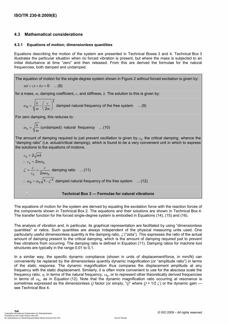
4.3.1 Equations of motion; dimensionless quantities

Equations describing the motion of the system are presented in Technical Boxes 3 and 4. Technical Box 3 illustrates the particular situation when no forced vibration is present, but where the mass is subjected to an initial disturbance at time “zero” and then released. From this are derived the formulae for the natural frequencies, both damped and undamped.

The equation of motion for the single-degree system shown in Figure 2 without forced excitation is given by:

0 ... (8)mx cx kx+ + =

for a mass, m, damping coefficient, c, and stiffness, k. The solution to this is given by:

2

d damped natural frequency of the free system ... (9)2

k cm m

ω ⎛ ⎞= − ⎜ ⎟⎝ ⎠

For zero damping, this reduces to:

(undamped) natural frequency ... (10)nkm

ω =

The amount of damping required to just prevent oscillation is given by cc, the critical damping, whence the “damping ratio” (i.e. actual/critical damping), which is found to be a very convenient unit in which to express the solutions to the equations of motions.

c

c n

c n

2d n

22

damping ratio ... (11)2

1 damped natural frequency of the free system ... (12)

c mkc m

c cc m

ω

ζω

ω ω ζ

=

∴ =

= =

∴ = −

Technical Box 3 — Formulae for natural vibrations

The equations of motion for the system are derived by equating the excitation force with the reaction forces of the components shown in Technical Box 2. The equations and their solutions are shown in Technical Box 4. The transfer function for the forced single-degree system is embodied in Equations (14), (15) and (16).

The analysis of vibration and, in particular, its graphical representation are facilitated by using “dimensionless quantities” or ratios. Such quantities are always independent of the physical measuring units used. One particularly useful dimensionless quantity is the damping ratio, ζ (“zeta”). This expresses the ratio of the actual amount of damping present to the critical damping, which is the amount of damping required just to prevent free vibrations from occurring. The damping ratio is defined in Equation (11). Damping ratios for machine tool structures are typically in the range 0,01 to 0,1.

In a similar way, the specific dynamic compliance (shown in units of displacement/force, in mm/N) can conveniently be replaced by the dimensionless quantity dynamic magnification (or “amplitude ratio”) in terms of the static response. The dynamic magnification thus compares the displacement amplitude at any frequency with the static displacement. Similarly, it is often more convenient to use for the abscissa scale the frequency ratio, η, in terms of the natural frequency, ωn, or to represent other theoretically derived frequencies in terms of ωn, as in Equation (12). Note that the dynamic magnification ratio occurring at resonance is sometimes expressed as the dimensionless Q factor (or simply, “Q” where Q = 1/2 ζ ) or the dynamic gain — see Technical Box 4.



--`,,```,,,,````-`-`,,`,,`,`,,`---

ISO/TR 230-8:2009(E)


The equation of motion for the harmonically forced single-degree system is:

0 sin ... (13)mx cx kx F tω+ + =

for an excitation force of amplitude, F0, and circular forcing frequency, ω, in rad/s. The reactive forces of the system on the left balance the exciting force on the right.

This is a “classic” second-order differential equation whose solution is given by the sum of the “Complementary Function” representing the initial transient and the “Particular Integral” representing the steady-state solution. The former is shown as:

n n(sin ) transient response ... (14)tx e A tζω ω ϕ−= −

and the latter shows the dynamic magnification and the resulting phase angle as a function of frequency.

( ) ( )2 20 2

12

1 dynamic magnification ratio ... (15)1 2

2tan phase angle ... (16)1

XX

η ζη

ζηϕη

−

=

− +

⎛ ⎞= ⎜ ⎟⎜ ⎟−⎝ ⎠

where

n frequency ratio ... (17)ωη

ω=

Formulae (15) and (16) represent the “transfer function” of the system.

For the transient formula, A = an arbitrary amplitude coefficient and ϕ = a phase angle. These values depend on the initial phase of the forced excitation at time t = 0.

For forced vibration, this becomes the resonance frequency, ωr :

21 2 ... (18)r nω ω ζ= −

And the maximum dynamic magnification ratio of the displacement amplitude at resonance is given by:

res 2

1 ... (19)2 1

Xζ ζ

=−

For small values of damping ratio, the dynamic multiplication factor at resonance, Q, reduces to: 1 ... (20)

2Q

ζ=

Technical Box 4 — Displacement equations of motion for forced second-order single-degree system

4.3.2 Energy considerations

A contrasting mathematical procedure for studying the behaviour of vibrating models is one using the balance of energy (see also 4.1.4). For example, the frequency Equation (10) can be derived alternatively by equating the maximum kinetic energy occurring at zero elongation to the maximum potential energy occurring at the maximum elongation.

4.3.3 Natural frequencies and resonance

A clear distinction should be made between the terms “undamped natural frequency”, “damped natural frequency” and “resonance frequency”. For zero damping, all these frequencies are identical and occur at the 90° phase point. When damping is present (which is always the case), the damped natural frequency [Equations (9) and (12)] is the frequency at which a system will oscillate freely, i.e. without external excitation.



--`,,```,,,,````-`-`,,`,,`,`,,`---

ISO/TR 230-8:2009(E)


This is always slightly lower than the (undamped) natural frequency [Equation (10)]. The resonance frequency [Equation (17)] is the maximum response (or dynamic compliance) to forced excitation and is slightly lower than the damped natural frequency. These two latter frequencies are dependent on the amount of damping present. For machine tool structures, where the damping ratio is generally less than 0,1, the differences between these three frequencies are academic and a quantitative distinction is not usually necessary. See Technical Boxes 3 and 4.

For frequencies ωu and ωl above and below resonance ωn, where response drops to 1 / 2 :

n

u l

for [from (17)]

bandwidth for 1 / 2 response

/ 2 ... (21)η

η

ωηω

η η

ζ

=

∆ = −

= ∆

The arrows drawn on the response in Figure 4 illustrate this concept, with the height of the arrows set at

1 / 2 of the peak and the measured width between them determining ∆ω .

Technical Box 5 — Practical calculation of damping ratio

As mentioned in 4.3.1, the dynamic magnification ratio occurring at resonance can also be expressed as Q, the dynamic gain — see Equation (20). Although the damping ratio may be derived theoretically from Q by computing the dynamic and static displacement amplitudes, this method is inappropriate for complex systems.

An alternative procedure is available for conditions of low damping. The two frequencies (either side of resonance), where the response is 1 / 2 times that at resonance, should be measured (perhaps graphically), and the values substituted in Equation (21) in Technical Box 5 to give an acceptable estimate of the damping ratio.

The solutions to Equations (15) and (16) allow useful graphical representations of a dynamic system to be constructed to provide a clearer understanding of its performance at different frequencies.

4.4 Graphical representations

4.4.1 Frequency response diagrams: dynamic magnification

A plot of the dynamic magnification is shown in Figure 4. It is a manifestation of the equations of motion in the frequency domain and shows the frequency response curve, i.e. Equation (15). It is also a plot of the magnitude of vector K, as it varies with frequency in Figure 3. In this particular case, the axes represent dimensionless quantities. The vertical axis shows the dynamic magnification ratio and the horizontal axis the frequency ratio in terms of the natural frequency. Frequency response diagrams of this kind are widely used for illustrating vibration behaviour and are not limited to single-degree systems. Other examples will be encountered later in Figures 6, 10, 11, 14, 15, 16, 19, 30, and elsewhere.

In Figure 4 two frequency responses of the system are plotted: (1) with low damping (ζ = 0,075) and (2) with high damping (ζ = 0,25). “ζ ” denotes the damping ratio (see 4.3.1). The value of 0,075 is quite typical for a machine tool. The higher value of 0,25 is, however, more representative of isolated damping elements, and it can be seen from this plot how significantly higher damping reduces the dynamic magnification at resonance. In Figure 4 resonance occurs close to the natural frequency, where the magnification ratio (or Q factor) is about 6,7 for (1), and 2,1 for (2). Consequently, the dynamic stiffness is 6,7 times less than the static stiffness. It will be seen that the frequency of maximum response (i.e. the “resonance frequency”, not the “natural frequency”) decreases slightly with increased damping.



--`,,```,,,,````-`-`,,`,,`,`,,`---

ISO/TR 230-8:2009(E)


4.4.2 Frequency response diagrams: phase

It is clear from the vector diagrams in Figure 3 and Equation (16) that the response is not fully described by the dynamic magnification plot alone. Over the frequency range covered for the model, the phase lag between the exciting force and the displacement is seen to shift from zero to nearly 180° and to be precisely 90° at the natural frequency. Note that since the velocity is always 90° ahead of the displacement, the phase between the velocity and the exciting force will range from 90° to 270°. Similarly, the phase of the acceleration to the exciting force will range from 180° to 360°. (Unless otherwise qualified, however, the phase is usually taken to be that between the displacement and the excitation force.)

In the frequency domain, the corresponding phase response diagram is shown in Figure 5. In addition, Figures 4 and 5, taken together, provide the necessary complete description of the response.

The phase angle shown in Figure 5 is representative of the angle of the force vector, F, in traces b) to e) of Figure 3. Traces 1 and 2 correspond to the same two values of damping factor shown in Figure 4. The third trace 3 shown in Figure 5 is the (almost) undamped response. Note that all the curves cross at the natural frequency, where the phase angle is always 90° and independent of damping.

Another way of presenting the phase “information” is to use two frequency response curves representing the real and imaginary parts of the dynamic magnification.

Key fr frequency ratio DM dynamic magnification 1 damping ratio, ζ = 0,075 2 damping ratio, ζ = 0,25

The significance of the arrows is discussed in Technical Box 5.

Figure 4 — Typical single-degree-of-freedom displacement responses for two values of damping ratio



--`,,```,,,,````-`-`,,`,,`,`,,`---

ISO/TR 230-8:2009(E)


Key fr frequency ratio PA phase angle (degrees) 1 damping ratio, ζ = 0,075 2 damping ratio, ζ = 0,25 3 damping ratio, ζ ∼ 0

Figure 5 — Single-degree-of-freedom phase response

Key fr frequency ratio DM magnitude of component response 1 real part 2 imaginary part ( j)

Figure 6 — Real and imaginary parts of complex displacement response for ζ = 0,075



--`,,```,,,,````-`-`,,`,,`,`,,`---

ISO/TR 230-8:2009(E)


4.4.3 Real and imaginary components of the response

In each of the diagrams of Figure 3, the vector F can be resolved into two components: an “in-phase” component parallel to K and a “quadrature” component at right angles, parallel to C. These components are usually referred to as the “real” and “imaginary” components respectively. (With their connotations of “mystery”, these unfortunate appellations contribute little towards the furtherance of clear understanding.) Figure 6 shows the two “component responses” of the dynamic magnification in the frequency domain. It can be seen that, at the natural frequency, the real component becomes zero. The two plots correspond to the single low damping plot in Figures 4, 5 and 6 (ζ = 0,075), and again provide a “complete description” of the response — this time in one diagram (but note that the phase is derivable only as a function of the two plots, and cannot be shown explicitly). On a machine tool, the value and frequency of the “maximum negative real part” are often significant factors in determining the frequency and possible severity of vibration to be encountered with the onset of chatter.

A further way of combining the phase and the dynamic magnification into a single plot is to use the “response vector locus” diagram.

4.4.4 Response vector locus diagram

This diagram is shown in Figure 7, again for the low damped plot from Figures 4, 5 and 6 (ζ = 0,075), and is essentially a reinterpretation of the series of vector diagrams shown in Figure 3. It is a plot in the complex plane, borrowed from control theory (whence its alternative name of “Nyquist” plot). Here, the real part is plotted on the abscissa against the imaginary part, plotted on the ordinate, with frequency as a curve parameter travelling clockwise around the locus from its start at the point (+1; j0), where the frequency is zero, towards its ultimate destiny at the pole where the frequency becomes theoretically infinite.

Figure 7 can also be interpreted as a polar plot. The radius of the response curve from the pole to any point and its angle (R, θ), i.e. its polar coordinates, give the dynamic magnification and phase angle respectively. Either way, this diagram provides a “complete description” of the response — except that the frequency values need to be marked along the curve, getting ever closer together as the frequency increases.

For a single-degree system, the undamped natural frequency occurs at the crossing of the loop with the imaginary axis (Im) while the resonant frequency occurs on the locus where R is maximum. From this diagram it can readily be seen that the resonance frequency, i.e. the maximum value of R, occurs just before the natural frequency.

For a more complex system with multiple resonances, it is possible for many loops to occur (which should be evaluated individually). When the excitation and measurement are at different locations or in different directions, the phase response may go beyond 180° and into the positive imaginary zone (see Figures 31 and 32).

The Nyquist criterion for servo stability can often be applied to chatter investigation. Briefly, this states that if the curve encloses the (–1, j0) point then instability (chatter) is likely. This can be identified with the “maximum negative real part” mentioned in connection with Figure 6.

Figure 8 shows the relationship of the force vectors shown in Figure 3 to the response vector locus diagram of Figure 7 at four selected frequencies.



--`,,```,,,,````-`-`,,`,,`,`,,`---

ISO/TR 230-8:2009(E)


Key Re real part Im imaginary part R dynamic response vector θ phase angle

Figure 7 — Displacement response vector locus for a single-degree-of-freedom system

4.5 Different types of harmonic excitation and response

In the single-degree of freedom model, only one type of excitation and response has been considered thus far: the displacement response to harmonic excitation applied to the “top” of the system, i.e. via the mass. Figure 9 shows a number of variations on this model having relevance to machine tool dynamics. In each of these models, the system is assumed to be standing on a very heavy inert surface or “ground” that does not take part in the vibration8).

4.5.1 Harmonic excitation through the mass: acceleration response

Figure 9 a) shows the system already discussed above whose absolute displacement response was shown in Figure 4. However, in this case the acceleration response is under investigation. This starts from zero and increases as the square of the displacement (Technical Box 2). Around resonance it is similar to the displacement response, but at high frequencies it approaches unity rather than zero. This is to be expected since, at very low frequencies, there is little acceleration whilst, at high frequencies, there is high velocity but this is offset by little displacement. The net effect is unit acceleration. The response is shown in Figure 10, where the ordinate shows the dynamic magnification of the acceleration and the equation for dynamic magnification is given by Equation (22). Such a response will be produced when the output of an accelerometer is measured directly.

8) Never strictly true! A consequence of the conservation of momentum is that the “ground” must always vibrate with the same momentum, see 4.1.4.



--`,,```,,,,````-`-`,,`,,`,`,,`---

ISO/TR 230-8:2009(E)


4.5.2 Out-of-balance excitation via the mass: absolute displacement response

In Figure 9 b), the system is excited by a rotating out-of-balance force vector (i.e. “centrifugal” force). The component of this force, acting to excite the mechanical system, is a sinusoidal force vector with a displacement proportional to the rotational velocity (or frequency) squared. Since acceleration is also proportional to velocity squared, it follows that this curve is the same shape as the response curve considered above in 4.5.1 (see Figure 10), but here the “magnification ratio” represents displacement. This model has relevance to excitation from out-of-balance motors and spindles9). See Equation (22).

4.5.3 Harmonic excitation via the base: relative displacement

Figure 9 c) shows the system inside a frame or “box” being excited via the base of the frame through a fixed absolute displacement amplitude, y. In this model, it is the resultant displacement amplitude, x, of the mass relative to the base that is of primary interest. The response curve for this is also shown in Figure 10, where “magnification ratio” now represents displacement amplitude ratio. At very low frequencies, the mass follows the motion of the base and exhibits very little relative movement. At high frequencies (above the natural frequency), the mass can no longer follow the base and becomes virtually stationary “in space”. This is because the relative motion of the mass becomes equal and opposite to that of the base.

This model has relevance to the application of accelerometer-type transducers, which operate well below their natural resonance. It should be noted that the fixed displacement amplitude criterion is valid only when the transducer has low mass and high stiffness relative to the machine tool.

See Equation (22) for the mathematical expression of the dynamic magnification.

9) The generation of out-of-balance forces is explained more fully in Clause 5.1.2.



--`,,```,,,,````-`-`,,`,,`,`,,`---

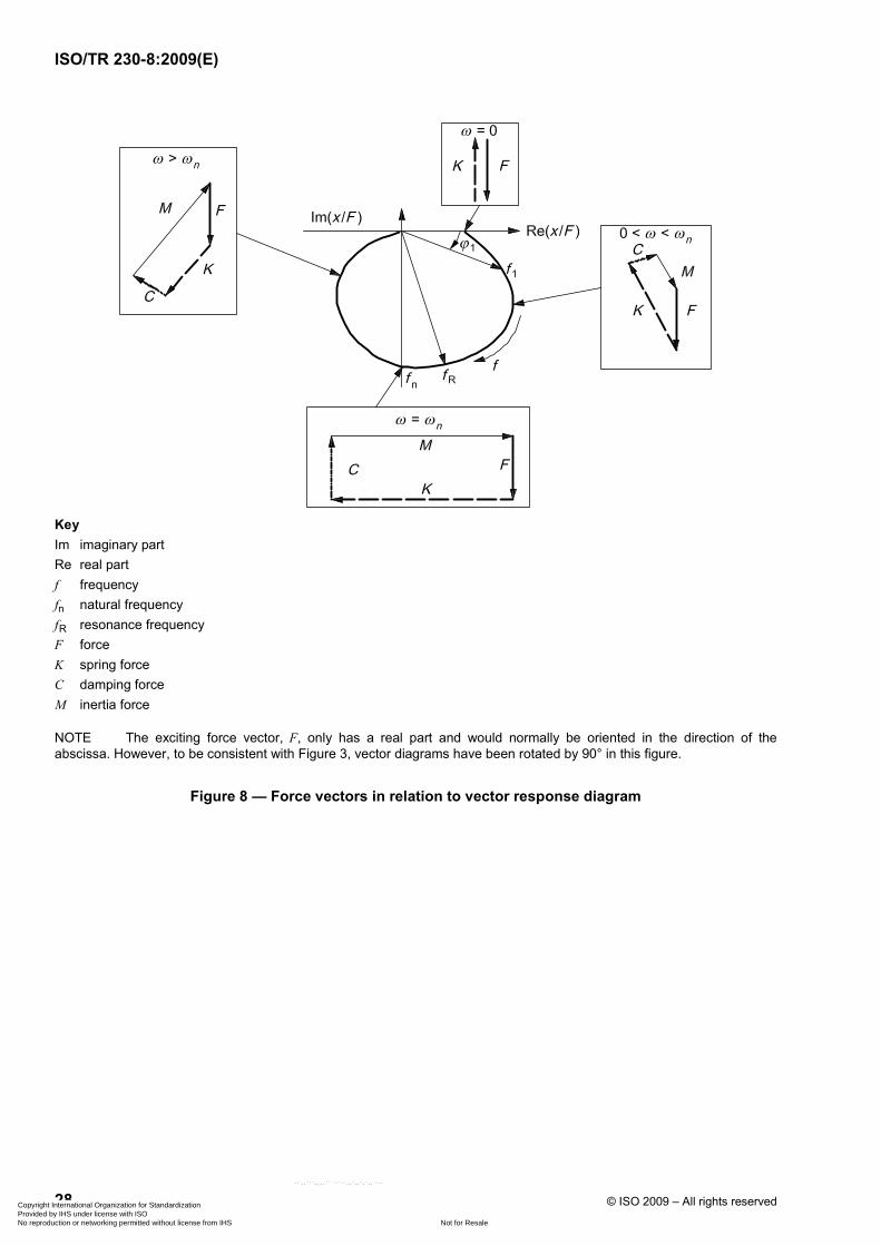
ISO/TR 230-8:2009(E)


Key Im imaginary part Re real part f frequency fn natural frequency fR resonance frequency F force K spring force C damping force M inertia force

NOTE The exciting force vector, F, only has a real part and would normally be oriented in the direction of the abscissa. However, to be consistent with Figure 3, vector diagrams have been rotated by 90° in this figure.

Figure 8 — Force vectors in relation to vector response diagram



--`,,```,,,,````-`-`,,`,,`,`,,`---

ISO/TR 230-8:2009(E)


a) Sinusoidally via mass b) “Centrifugally” via mass

c) Sinusoidally via base of frame measured relatively

d) Sinusoidally via base measured absolutely

Figure 9 — Various cases of excitation of a single-degree-of-freedom system



--`,,```,,,,````-`-`,,`,,`,`,,`---

ISO/TR 230-8:2009(E)


Key fr frequency ratio MR magnification ratio 1 damping ratio, ζ = 0,075 2 damping ratio, ζ = 0,25

Figure 10 — Absolute displacement response of single-degree-of-freedom system excited through unbalance; relative displacement of system excited through its base;

or acceleration response of the system excited through the mass

4.5.4 Harmonic excitation via the base: absolute displacement; transmissibility

Figure 9 d) is similar to Figure 9 c) except that only the base of the frame is shown. This is because it is the absolute displacement amplitude, y, of the mass that is now of interest. The displacement magnification response to this is shown in Figure 11 and is called the transmissibility.

Figure 11 should not be confused with Figure 4, to which it is superficially similar. Indeed, the forces acting on the mass, K, M and C, are essentially the same as before except that K and C are now measured relative to the base movement, whereas M is always absolute. At low frequencies, the mass moves by the “static” amount, y, “in space”, but is stationary relative to the base. At high frequencies, with little or no damping, the mass moves very little “in space” because of its inertia. In this plot, however, a higher value for the larger damping ratio (trace 2) has been used (ζ = 0,7) in order to highlight the difference between this and Figure 4. (Trace 2 still corresponds to ζ = 0,075.) At high frequencies (i.e. specifically above 2 × natural frequency), the increased damping couples the mass more securely to the base of the frame and its absolute movement does not therefore decline so readily. Note that all the curves, whatever the damping, exhibit unit response at

2 × natural frequency, which is their point of mutual intersection. For very high damping and very high frequencies, the response tends towards unity rather than zero. See Equation (23).

This model has relevance to the isolation of a machine standing on a vibrating floor that is too massive in itself to be influenced much by the machine. (See 4.1.4 for energy and momentum considerations, and also Footnote 9 in 4.5.)

Transmissibility works both ways: vibration can be induced by the floor into the model (i.e. the machine) or by the machine into the floor, and the above arguments apply equally to both situations.

The performance of isolation mounts can be understood from Figure 11. At all frequencies below the critical value of 2 × natural frequency, some amplification of the floor movement by the machine is inevitable, though increased damping will help to limit this, particularly when close to resonance. Above this critical frequency, there is always some attenuation and this increases with frequency.



--`,,```,,,,````-`-`,,`,,`,`,,`---

ISO/TR 230-8:2009(E)


It is evident from the figure that very high damping will ensure a flat response over the complete range, since the machine is virtually “glued” to the floor. This means that, in this case, increased damping is actually counter-productive. Obviously, some sort of compromise involving a moderate amount of damping is required to cope with real situations, particularly where machine natural frequencies are likely to be excited by the floor.

Key fr frequency ratio TR transmissibility 1 damping ratio, ζ = 0,075 2 damping ratio, ζ = 0,70

Figure 11 — Transmissibility response

For excitation via the spring support, the force applied to the mass is proportional to the square of the frequency. This is equivalent to direct excitation through the mass by an unbalance force. The dynamic magnification is:

( ) ( )

2

2 20 2 ... (22)

1 2

XX

η

η ζη=

− +

NOTE Equation (22) also represents the acceleration response for direct excitation of the mass.

For the transmissibility factor between floor and machine, the dynamic magnification is:

( )

( ) ( )

2

2 20 2

1 2 ... (23)

1 2

XX

ζη

η ζη

+=

− +

Technical Box 6 — Excitation through unbalance and transmissibility



--`,,```,,,,````-`-`,,`,,`,`,,`---

ISO/TR 230-8:2009(E)


4.5.5 Excitation through impulse: free and transient vibrations

In the foregoing discussions on sinusoidal excitation, only the steady-state solution to the equations for forced vibration has been considered. Under these conditions, the system always vibrates at the same frequency as the excitation force.

Without a forcing frequency, vibrations can still occur at the damped natural frequency whenever the system is disturbed from its quiescent state (see Technical Box 3). The exponentially decaying sine wave shown in Figure 12 (trace 1) is a typical response in the time domain. Such a response could be generated by a single impulse, e.g. from striking a bell. This is known as transient vibration and is represented by the transient response formula shown in Equation (14).

From Equation (14) it can be seen that the rate of exponential decay depends on both the damping ratio and the natural frequency: the decay is faster for high frequencies and for high damping. The damping effect consequently becomes much less efficient at low natural frequencies. Such frequencies (representing the lowest modes of vibration10) of the machine) can then persist for several seconds after the disturbing impulse has been removed. This has relevance to the behaviour of machine structures following rapidly accelerating or decelerating machine feed slides.

A similar situation occurs when harmonic excitation is initiated from rest. The system cannot instantly respond to the excitation because the rest state does not correspond to the any of the dynamic states shown in Figure 1. For nowhere in that diagram are the acceleration, velocity and displacement all zero at the same time. The moment of initiation is in fact similar to that of the single impulse. It too is therefore governed by the transient response.

Key t time Iv instantaneous value 1 free motion 2 forced motion 3 resultant motion

Figure 12 — Starting transient for forced vibrations

10) Machine “modes” are discussed later in 4.6.4.



--`,,```,,,,````-`-`,,`,,`,`,,`---

ISO/TR 230-8:2009(E)


Figure 12 shows what happens. The “resultant motion”, 3, is the sum of the “free motion”, 1, and the “forced motion”, 2. The example shows a forced vibration with an excitation frequency of about 1/5th of the system’s natural frequency. At the start of the excitation, free vibrations at the damped natural frequency dominate the motion, and are automatically superimposed onto the forced excitation so that the two displacements just cancel. This “allows” the “resultant motion” of the system to start from rest. Initially then, there is a mix of both natural and excitation frequencies. The free motion (at the natural frequency) then dies away as shown in 4.5.5 as the steady-state excitation frequency eventually comes to dominate the motion. The time required for this to happen depends on the damping and the natural frequency. When the excitation force is removed, the system will automatically revert to its free vibration state, as discussed previously.

4.6 More degrees of freedom

4.6.1 Two degrees of freedom: modes

The next step up from the single-degree-of-freedom system shown in Figure 3 is the two-degree-of-freedom system where an additional mass and spring are attached to the main mass, which is being excited. Two possible configurations are shown in Figure 13, with m1 and m2 indicating the two masses.

a) Masses m1 and m2 both grounded b) Mass m2 fixed to m1 only

Figure 13 — Two types of two-degree-of-freedom system

These configurations add another degree of freedom to the system because it can now oscillate in two distinct ways, or modes, with the two masses moving in either similar or contrary motion. There are now two independent displacement amplitude variables, x1 and x2, each associated with a particular mass. To facilitate the explanation, the simple undamped model shown in Figure 13 a) should be envisaged with two equal masses, m, and two equal springs, k (top and bottom), with a “soft” coupling spring, k0, between them.



--`,,```,,,,````-`-`,,`,,`,`,,`---

ISO/TR 230-8:2009(E)


In this case, it is evident that a mode can exist where both masses can be set moving in the same direction such that k0 neither extends nor compresses, i.e. x2 = x1. The natural frequency for this mode is determined simply by the value of k [as in Equation (10)]. Alternatively, if the midpoint of k0 is fixed then both masses can be set oscillating in opposite directions, i.e. x2 = –x1, again both at the same frequency. The natural frequency for the second mode is determined by the increased spring constant (k + k0/2), and is clearly higher than that for the first mode. (Note that other modes can exist, but only as transients.)

There are now also two choices of mass for the point of excitation and two choices for the point of measurement. The frequency response in Figure 14 shows the behaviour of a two-degree-of-freedom system similar to that in Figure 13 a), where both masses are nearly (but deliberately not quite) the same. In this example, with almost zero damping, it is possible to incorporate the phase into the response by always making its value either zero (positive response) or 180° (negative response). Frequencies are now shown as ratios in terms of the natural frequency of the one mass on its own as a single-degree-of-freedom system. It can be seen from the plot that both masses are in phase for the lower resonance (centre spring not extending), and in antiphase for the upper resonance (centre spring stationary at its midpoint). It is also seen that, at frequencies between these two resonances, the movement will consist of a mix of the two modes, but, of course, with much reduced dynamic magnification ratios. Note that, at the original resonance (frequency ratio ~1), the displacement amplitude becomes zero for mass 1.

Key fr frequency ratio DM dynamic magnification 1 mass 1 2 mass 2

Figure 14 — Displacement response in a two-degree-of-freedom system with low damping [as in Figure 13 a)]

4.6.2 Vibration absorbers

A special case of the two-degree-of-freedom model relevant to machine tools is illustrated in Figure 13 b). This is the dynamic vibration absorber, where the second mass/spring/damper system is attached directly to the first system and not to “ground”. Although theory, confirmed by experiments, shows that the auxiliary mass should be as large as design considerations may permit, it is generally unfeasible to make it larger than 1/10th to 1/5th of the equivalent mass of the mode to be damped. The auxiliary mass system should be “tuned” to have approximately the same individual natural frequency as the main mass system. Note that unlike the main system, which is excited directly, the auxiliary system is excited through its base [compare with Figure 9 d)]. Figure 15 shows the frequency response of the main mass for this case.



--`,,```,,,,````-`-`,,`,,`,`,,`---

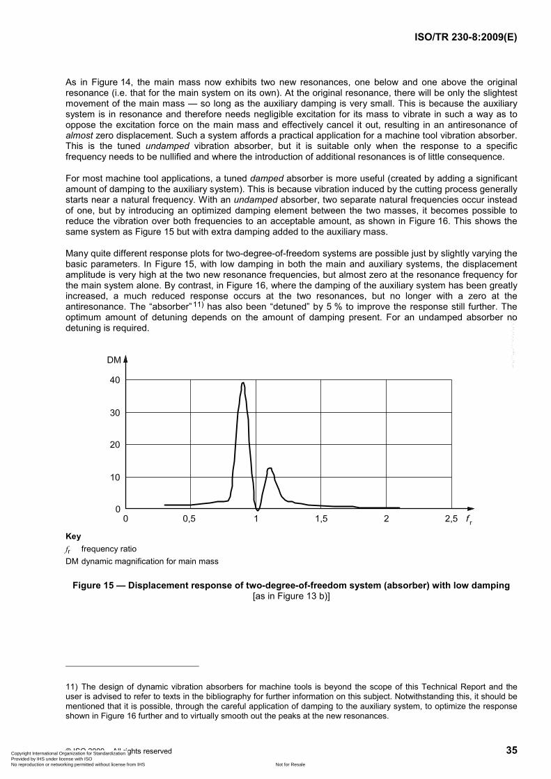
ISO/TR 230-8:2009(E)


As in Figure 14, the main mass now exhibits two new resonances, one below and one above the original resonance (i.e. that for the main system on its own). At the original resonance, there will be only the slightest movement of the main mass — so long as the auxiliary damping is very small. This is because the auxiliary system is in resonance and therefore needs negligible excitation for its mass to vibrate in such a way as to oppose the excitation force on the main mass and effectively cancel it out, resulting in an antiresonance of almost zero displacement. Such a system affords a practical application for a machine tool vibration absorber. This is the tuned undamped vibration absorber, but it is suitable only when the response to a specific frequency needs to be nullified and where the introduction of additional resonances is of little consequence.

For most machine tool applications, a tuned damped absorber is more useful (created by adding a significant amount of damping to the auxiliary system). This is because vibration induced by the cutting process generally starts near a natural frequency. With an undamped absorber, two separate natural frequencies occur instead of one, but by introducing an optimized damping element between the two masses, it becomes possible to reduce the vibration over both frequencies to an acceptable amount, as shown in Figure 16. This shows the same system as Figure 15 but with extra damping added to the auxiliary mass.

Many quite different response plots for two-degree-of-freedom systems are possible just by slightly varying the basic parameters. In Figure 15, with low damping in both the main and auxiliary systems, the displacement amplitude is very high at the two new resonance frequencies, but almost zero at the resonance frequency for the main system alone. By contrast, in Figure 16, where the damping of the auxiliary system has been greatly increased, a much reduced response occurs at the two resonances, but no longer with a zero at the antiresonance. The “absorber”11) has also been “detuned” by 5 % to improve the response still further. The optimum amount of detuning depends on the amount of damping present. For an undamped absorber no detuning is required.

Key fr frequency ratio DM dynamic magnification for main mass

Figure 15 — Displacement response of two-degree-of-freedom system (absorber) with low damping [as in Figure 13 b)]

11) The design of dynamic vibration absorbers for machine tools is beyond the scope of this Technical Report and the user is advised to refer to texts in the bibliography for further information on this subject. Notwithstanding this, it should be mentioned that it is possible, through the careful application of damping to the auxiliary system, to optimize the response shown in Figure 16 further and to virtually smooth out the peaks at the new resonances.



--`,,```,,,,````-`-`,,`,,`,`,,`---

ISO/TR 230-8:2009(E)


The careful installation of tuned dynamic absorbers has been shown to enhance machine performance considerably by permitting higher metal-removal rates to be achieved before the onset of self-excited vibrations (chatter). Absorbers of this kind are usually tuned to approximately the frequency of the vibration mode identified with chatter.

NOTE The formula for this system in dimensionless quantities is given in Technical Box 7; the dimensionless values used in constructing Figures 15 and 16 are shown in Table 1.

Key fr frequency ratio DM dynamic magnification for main mass

Figure 16 — Response of two-degree-of-freedom (absorber) system with increased auxiliary damping [as in Figure 13 b)]

The choice of placement of vibration absorbers on machines should preferably be governed by energy or momentum considerations. They should ideally be placed where the energy level is greatest, and not necessarily where the greatest displacement amplitude is observed. For instance, the vibration of a machine tool could manifest itself greatly in the vibration of a lightweight panel (e.g. a cabinet door). Because such a panel has a low energy level (i.e. low mass), applying damping to it would succeed only in reducing the vibration of the panel and have minimal effect on the machine as a whole.

Equation for a two-degree system with damping in both parts. For a main system (m), M, K, C, and an auxiliary system (a), m, k, c, the response of the main system at a circular frequency, ω, is obtained from Equation (24):

( ) ( )( ) ( ) ( ) ( )

22 2 2a

2 20 2 2 2 2 2 2 2 2 2 2 2a a

a

2 ... (24)

2 1 1 4mm

f g g fXX

f g g g g f f g g g f g ff

ζ

ζζ µ µ ζ ζ

ζ

× + +=

⎡ ⎤ ⎡ ⎤× − + + − + − − − +⎢ ⎥ ⎢ ⎥⎣ ⎦⎣ ⎦where

aa m a m

m m; ; ; ; ; ;

2 2c C k K mf g

m M Mkm KMω ωζ ζ ω ω µω ω

= = = = = = =

Technical Box 7 — Two-degree absorber system with damping



--`,,```,,,,````-`-`,,`,,`,`,,`---

ISO/TR 230-8:2009(E)


Table 1 — Dimensionless parameters used for Figures 15 and 16

Figure No. 15 16

Mass ratio (auxiliary/main) (µ) 0,05 0,05

Ratio of natural frequencies (auxiliary/main) ( f ) 1,00 0,95

Damping ratio of main system (ζm) 0,001 0,001

Damping ratio of auxiliary system (ζa) 0,001 0,10

4.6.3 Multi-degree-of-freedom systems and distributed systems

Multi-degree-of-freedom systems can be envisaged as extensions to the foregoing, with many masses and springs connected in endless varieties of configuration. With more degrees of freedom, movement can occur in two, or even three, spatial dimensions and can include rotational (i.e. torsional) elements as well as the linear movements discussed here.

4.6.4 Machine tools: machine modes

In a system as complex as a machine tool, however, it becomes increasingly difficult to model the machine in this way because its mass, stiffness and damping are not separate entities, but are distributed throughout the structure. The mathematical treatment of such a system is beyond the scope of this part of ISO 230, and it may not even be necessary for much practical test work. Modelling of complex systems for design purposes is nowadays carried out using the numerical technique of “finite element analysis”. To do this adequately for a complex machine can take many hours of computation time even with modern high-speed processors.

Suffice it to say that such complex systems would be expected to exhibit many modes, each with its own natural frequency. Whilst this is true, it turns out that, for most machine tools, only a relatively small number of these possible modes are significant enough to warrant investigation. Often, this means that the dynamic behaviour of the machine can easily be described mathematically by assuming the characteristics of a linear system. If the modes occur at sufficiently widely separated frequencies, it is possible to treat them as individual single-degree-of-freedom systems, each with an equivalent (or “modal”) mass, spring and damper as in the single-degree models discussed earlier. The frequency response function of the machine then becomes the sum of the frequency response functions of the equivalent single-degree-of-freedom systems, each representing a specific natural frequency of the system — see Technical Box 8. (Graphically, an equivalent procedure known as “mode splitting” can be carried out on the complex response vector locus diagram — see Figure 7.)

( ) 0i2

ii

ni ni

... (25)

1 2

GG j

j

ωω ωζω ω

=⎛ ⎞

+ − ⎜ ⎟⎝ ⎠

∑

where ωni is the natural frequency of the i th mode of the system

and ζ i is the damping ratio of the i th mode

and G0i is the dynamic compliance of a single-degree-of-freedom system of the i th mode, and represents the complex quotient of displacement and the respective dynamic force.

Technical Box 8 — Summation of responses for a machine tool

With a machine tool there are, of course, opportunities for measurement and excitation at many different locations, and in a number of different directions. This means that there can be many different values for dynamic stiffness (or many different transfer functions). In general, though, the most important location for measuring dynamic stiffness on a machine tool is between the workpiece and the tool, because it is here that vibration is most likely to adversely affect the finished workpiece. Measurement of response is not, of course, restricted to the location of the excitation. (In fact, the locations of the excitation and of the measurement can



--`,,```,,,,````-`-`,,`,,`,`,,`---

ISO/TR 230-8:2009(E)


usually be interchanged without altering the response characteristics.) Figure 32 shows a matrix of dynamic compliance values or transfer functions for each direction of excitation combined with each direction of measurement.

It is important to understand that forced excitation at any point on the machine will, in principle, generate a vibration response at all other points on the machine. (Response measurements in locations and/or directions different from that of the excitation are generally referred to as “cross-response tests — see 8.6.) The resulting amplitude of the vibration displacement depends on the frequency of excitation and the location of the point. As with the simple models discussed above, for sinusoidal excitation, the steady-state vibration response will always be at the same frequency as the excitation. Taken collectively, the various displacement amplitudes (and phases) of vibration at discrete points over the structure will evince the characteristic modal “shape” of the machine for that frequency.

Modes can occur in all three dimensions and sometimes they may be “close coupled” which means that the vibration energy can “wander” back and forth between the two modes12). [Two pendulums tuned to almost the same frequency and suspended from the same frame exhibit this property: first one swings, then the other. Because of the conservation of momentum (see 4.1.4), the frame itself can never be entirely stationary and this provides the means of transferring the momentum.] The existence of coupled modes can sometimes be an important underlying factor in the development of chatter.

Figure 17 shows two views of a basic vertical machine tool with two carrier positions (high and low) illustrated. Diagrams a) and b) show the side and front views, respectively, of the quiescent machine. Note that the carrier height has an important influence on the modal stiffness (see 4.6.5). Figure 18 shows the same machine exhibiting two possible vibration modes, each one shown from the view that illustrates it best.

Each mode will have its own resonance where the response shows a maximum. Like the two-degree-of-freedom system (Figure 15), the modes at the lowest frequencies are quite simple with large “lumps” of the machine moving more or less together in phase. A very common mode for this type of machine is known as the “C frame” mode13), and is illustrated in Figure 18 a). This shows the column bending from the base and causing the spindle carrier to rotate forwards and downwards in the vertical plane. This mode clearly involves a lot of moving mass: the spindle carrier and the upper part of the column. The carrier is shown in its upper position, where it will generate the weakest (i.e. lowest frequency) version of this mode.

As the frequency is increased, this simple modal pattern breaks up as the more inert parts of the machine begin to lag behind. Figure 18 b) shows another likely mode where the spindle carrier is twisting on the column. In many types of vertical machining centre, this mode generally involves less mass and more stiffness, and, where this is the case, this mode would probably appear at a frequency somewhat higher than that of the “C frame” mode, and also be much less influenced by the height of the spindle carrier.

In practice, many more modes will exist than can be shown here, such as the carrier bending from side to side on the column (horizontally) and the column twisting about its base. As a general rule, it will be found that all parts of the machine are likely to exhibit some vibration in every mode.

At higher frequencies still, the modes become increasingly complex with many separate parts moving in different directions. Higher frequencies need more energy to excite them and result in smaller displacement amplitudes. It should be recognized that, while certain modes are usually associated with particular natural frequencies and modal analysis (see 8.5) is directed towards evaluating the characteristics of these modes, there is actually a gradual transition through the discrete modal shapes over the whole frequency range. At frequencies between resonances, mixed modes will occur, though these are generally of less interest to the tester because the displacement amplitudes are very much smaller.

The modes exhibited by a machine tool depend on the location and direction of the exciting force. Both the modes illustrated in Figure 18 involve relative movement between the tool and workpiece, and could therefore be excited by the cutting process, or even by an artificial exciter placed between the tool and the workpiece,

12) These modes are “close” in the sense that their frequencies are numerically close.

13) This type of structure is often known as a “C frame” because of its similarity to the letter. It is the shape of the “C” that undergoes distortion in this mode.



--`,,```,,,,````-`-`,,`,,`,`,,`---

ISO/TR 230-8:2009(E)


arranged so that the exciting force had the same direction as the cutting force14). For a machine tool, this will therefore generally be the most suitable point for excitation, but it does mean that any modes that have a node at this point cannot be excited. Many modes can exhibit one or more nodes. These are points or lines on the surface where there is virtually no movement, but where points on either side have movements 180° out of phase with one another. For instance, probes placed at the top and bottom of the carrier in Figure 18 b) (at positions and directions indicated by “1” and “2”) will at any instant register opposite phases. And at some point between these positions there will be a node. An exciter placed at the node cannot excite this mode because there is no movement and the structure thus appears to be infinitely stiff. Likewise, placing an exciter at right angles to the direction of modal movement will have no effect.

Such modes can still, of course, be excited from other locations and may need to be investigated if found to be troublesome — see 5.5.

4.6.5 Machine tools: effect of slide positions

Clearly, for any particular mode, the positions of the movable linear slides within the workspace (and hence the positions of the associated structural elements) will influence the modal mass as well as the static stiffness. If the spindle carrier is positioned at the top of a column, this will create a much weaker dynamic system than it would if positioned lower down (compare the two positions shown in Figure 17). A weaker dynamic system means lower natural frequencies and greater displacement amplitudes. It is thus most essential to record the axial positions of all slides before carrying out any type of vibration test.

Avoidance of major resonances in a machine tool is desirable, but rarely achievable. The next best thing is to minimize the dynamic magnification at the major resonances. Two factors should be borne in mind: frequency and damping. Higher frequencies take more energy to excite them than lower ones; they also die away much more quickly when the excitation is removed. Improved dynamic performance can thus be achieved by raising the natural frequencies, which effectively means increasing the static stiffness and/or reducing the modal mass of machine elements. It also follows that working with the carrier in its lowest feasible position (as in Figure 17) makes good sense.

a) Side view b) Front view

Figure 17 — Two views of a basic machine tool showing two carrier positions

14) As this is often not easy to realize on an actual machine tool, mathematical methods can be used to combine the loci of the artificial excitation exerted in x, y and z directions.



--`,,```,,,,````-`-`,,`,,`,`,,`---

ISO/TR 230-8:2009(E)


a) Column bending b) Carrier twisting

Figure 18 — Two possible vibration modes of the machine tool shown in Figure 17 (“1” and “2” show probe positions referred to in 4.6.4)

4.7 Other miscellaneous types of excitation and response of machine tools

Basic excitation and response of simple systems have been discussed in 4.5. In this clause, more “advanced” examples are considered.

4.7.1 Complex excitation: Fourier analysis

The waveform of the exciting force is dependent on its method of generation (see Clause 5). Up until now, the excitation has been assumed to be both periodic and harmonic. This means that a corresponding harmonic (i.e. sinusoidal) response of the same frequency and waveform results all over the structure, even though the amplitude and phase generally vary from point to point. This is not the case, however, when the waveform of the exciting force is no longer sinusoidal.

All repeating (i.e. periodic) wave patterns can be broken down, by Fourier analysis, into a series of harmonics. These are sine waves with frequencies that are integer multiples of the underlying or fundamental frequency. Each harmonic has its own amplitude and phase that are fixed relative to the fundamental wave. Analysis of complex15) waves into their harmonics is usually an automatic function of frequency analysis equipment. As a complete Fourier transform requires a long processing time, the Fast Fourier transform, or FFT algorithm, is used as a good practical alternative. (If the complex wave can be represented by mathematical formulae, then Fourier analysis can also usually be carried out mathematically.)

The response of a machine to a complex waveform will be the resultant of its responses to each of the individual harmonic components. Thus, for example, the response to harmonics close to a resonance will be much greater than to those further away. This means that relative magnitudes (and phases) of the harmonics in the response will now be different from those in the excitation signal, being enriched by frequencies close to resonances. This new harmonic “mix” provides the “ingredients” for a new waveform that now appears in the response. Furthermore, the modified waveform will vary over the structure, mirroring the way that the dynamic stiffness also varies over the structure.

So, for a complex excitation consisting of many harmonic components, the response of the structure will disproportionately amplify those that are close to its resonances. The response waveform thus becomes dominated by these resonances.

15) Strictly a “multi-sinusoidal waveform”.



--`,,```,,,,````-`-`,,`,,`,`,,`---

ISO/TR 230-8:2009(E)


It is important to understand that the machine is able to vibrate only at frequencies present as constituents of the excitation signal. However, a frequency present in quite a small proportion may be amplified many times more than another frequency already present in a moderate proportion. Because of this, when a machine is excited by a complex signal, it will respond mainly at frequencies where its dynamic stiffness is lowest, i.e. nearly (but not usually exactly) equal to its natural frequencies.

In some cases, the excitation may not even be periodic.

4.7.2 Aperiodic excitation

Many signals are in fact non-periodic. Impulses and steps (whether from accelerating slides or instrumented hammers), random noise generators or feedback from unstable cutting processes all generate highly complex waveforms with no underlying periodicity, and sometimes even with discontinuities. It was shown in 4.5.5 how single impulses could generate transient responses at the natural frequency. Discontinuities in excitation have the same effect. The Fourier analysis of steps, impulses and the like reveals signals rich in harmonics, with virtually every frequency present. Consequently, the same effect is produced by this type of excitation as would result from simultaneously exciting all possible frequencies over a wide range. In other words, the resultant response is effectively the same as the frequency response obtained by summing the results of applying a sine wave excitation and slowly scanning through all the frequencies: it results in the consequent domination of the response by the natural frequencies.

This characteristic is exploited when taking a frequency response measurement (see 8.4). Using composite excitation signals allows a much faster frequency response to be made than could be achieved by checking each frequency individually with sine wave excitation. In order for this technique to work, it is necessary to know the spectrum of the excitation signal as well as that of the response, so that the relationship between the response and the excitation (i.e. transfer function) can be evaluated throughout the frequency range.

4.7.3 Non-linear stiffness

It is possible for certain machine modes to exhibit non-linearity. Non-linearity means that the coefficients of stiffness, k, and of damping, c, are not constant over the whole range of deformation but increase or decrease more than or less proportionally with elongation. Non-linearity can apply to both stiffness and damping, but in the present context it is only the non-linearity of stiffness that is generally of interest. This is most likely to be encountered in the so-called “stiffening system” where the stiffness increases with displacement, and can be experienced when testing machines with unbalanced spindles by first accelerating then decelerating the spindle. Figure 19 shows the frequency response of such a system, with the full line showing the theoretical “mathematical” locus of the stiffening function16). In practice, the response cannot be “reversed” and hence discontinuous jumps occur. When the speed is gradually increased to just beyond the resonance point — where the curve reverses —, the displacement amplitude falls abruptly, following the right hand vertical dashed line and then picks up the response locus lower down. Likewise, if the speed starts above resonance and decelerates gradually towards resonance, the response will “jump” up the left-hand dashed line with a resonance reappearing just as abruptly, but at a lower speed, and with a lower amplitude than when accelerating. (The opposite effects happen in the much less commonly encountered “softening system”, where the response curve is essentially the mirror image of Figure 19. Here, resonance appears abruptly on accelerating, and at a lower speed than when decelerating.)

If the spindle speed is close to resonance, but fluctuating slightly, this phenomenon can result in the vibration disappearing and reappearing (often with changing displacement amplitudes) apparently at random. In this case, “chaotic” conditions can prevail, with an indeterminate response prevailing in the zone between the dashed lines.

Non-linearity of this kind tends to be a function of high force levels and is often absent at the levels used for frequency response testing. Since it occurs as a result of gradually increasing (or decreasing) the frequency of harmonic excitation, it is unlikely to be identified by using stochastic excitation techniques.

16) For convenience, in this frequency plot, the frequency scale is in “real” units rather than dimensionless ratios. The choice of scale depends on usage.



--`,,```,,,,````-`-`,,`,,`,`,,`---

ISO/TR 230-8:2009(E)


Key f frequency (Hz) DM dynamic magnification

Figure 19 — Typical frequency response of a non-linear stiffening system showing amplitude ratio against absolute frequency in hertz

Non-linearity is a complex subject involving some quite advanced mathematics. However, it is a phenomenon that can occur on machine tools, where it may be the cause of puzzling and unexplained test results. It is introduced here for the sole purpose of alerting its existence to the test engineer who will recognize it when encountered.

4.7.4 Practical damping

4.7.4.1 General

Damping is the force that limits the build-up of displacement amplitudes at resonance by effectively removing energy17) from the vibrating system. It is present in varying degrees intrinsically in all materials: those that “ring” when struck have less damping than those that do not; for example, cast iron has more damping than steel, which is why it is quite unsuitable for making bells. However, in machine tools, much of the damping actually comes from the friction between the interfaces of the structural elements (e.g. bearings, weldments, bolted joints) rather than intrinsically from the material itself. The actual friction present at these interfaces will vary with the amount of lubrication and the degree of wear present, and also with the relative locations of sliding covers and movable slides.

NOTE In all types of friction damping, some motion between two constructional parts is required, which may induce an accuracy error. This highlights the real advantage of trying to use a damped vibration absorber, because the motion then takes place in the secondary loop.

Damping also influences the way vibrations die away when the excitation is removed (see 4.5.5 for more details).

Damping generally varies from mode to mode and this has an influence on the shape of the frequency response. Low damping produces sharp peaks with narrow bandwidths; high damping produces rounded peaks with much wider bandwidths. This can be seen from the two traces in Figure 4, and can also be derived

17) And converting it into molecular energy, i.e. heat.



--`,,```,,,,````-`-`,,`,,`,`,,`---

ISO/TR 230-8:2009(E)


from Equation (21). (Note that whilst zero damping theoretically results in an infinite displacement amplitude at the natural frequency, there is still a finite response at all frequencies that are not precisely equal to the natural frequency.) The introduction of further damping can be achieved by the installation of either friction dampers or custom-designed “tuned damped absorbers” — see 4.6.2.

4.7.4.2 Viscous and non-viscous damping

It should be understood that viscous damping (which has been mentioned in previous clauses) is an idealized mathematically engineered concept. Its only property is that it generates a reaction force directly proportional to velocity (and opposite to it) and is therefore strictly linear. In reality, damping rarely behaves precisely like this, but the concept is nevertheless close enough to reality to be useful in machine tool vibration work where the degree of damping is usually quite low. The numerical evaluation of the damping ratio, ζ, in 4.3.1 and Technical Box 3 is likewise strictly valid only for truly viscous damping, but it is nevertheless still quite generally used because of its convenience. The closest practical realization of viscous damping is the hydraulic dashpot. Other types of damping that may be encountered are “magnetic” damping, “hysteretic” damping and “Coulomb” damping. Only the last of these will be considered here.

4.7.4.3 Coulomb damping

Coulomb damping (or dry friction damping) is common in machine tools and is quite different from viscous damping. Remember that viscous damping is directly proportional to the velocity of motion, which it opposes. Coulomb friction occurs between components held together by a certain level of clamping force. With very light clamping, the two components can move relative to one another with little damping. With heavy clamping, the two components move as one, again with no damping. But under intermediate levels of clamping, relative slip between the components can occur, which absorbs energy from the system through friction. Machine tool vibration absorbers (e.g. for milling machines and boring bars) have been successfully used for many years based on this principle. Coulomb damping can be a cause of non-linearity.

4.7.4.4 Negative damping

Occasionally, it is possible for dry friction to promote negative damping. The mechanism for this is related to the phenomenon of stick-slip where friction increases with decreasing velocity, and where static friction is greater than dynamic. By almost cancelling out the “natural” damping, this can allow very high displacement amplitudes at resonance to occur. The action of a violin bow on a string falls into this category; so does the squeal of a chalk on a blackboard. And in machine tools a similar effect can occur between a cutting edge and the workpiece material, which can thus initiate chatter. The slight dulling of the cutting edge with wear is often an antidote to this condition.

4.8 Spectra, responses and bandwidth

4.8.1 Spectrum analysis and frequency response

The various frequency response diagrams presented in this clause are based on theoretical considerations only. The practical realization of creating such diagrams through measurement is covered in Clause 8. It should be understood that the measurement of any frequency-related vibration data of this kind requires some form of spectrum analysis. At its simplest this means that the vibration power is evaluated in a series of predetermined bandwidths over the range of interest. The result of this is often superficially similar to a frequency response test, but note that, to create a complete frequency response graphic, it is necessary to carry out two spectrum analyses simultaneously, one on the excitation signal and one on the response, and to keep track of their relative phases. This allows both the amplitudes and phases of the two waves to be compared at each “bandwidth”.

4.8.2 Bandwidth and power

Bandwidth is an important concept in the measurement of vibration spectra, and this applies to both the signal being measured and to the response of the equipment used for measurement. For a signal, the “bandwidth” is simply the frequency range within which the amplitude of the signal exceeds a particular threshold. For example, in the estimate of damping ratio shown in Technical Box 5, the threshold level is 1 / 2 of the peak



--`,,```,,,,````-`-`,,`,,`,`,,`---

ISO/TR 230-8:2009(E)


value and the bandwidth is defined by the upper and lower frequencies either side of the peak corresponding to this level. For measurement equipment response, the bandwidth relates to the limit of the measurement range, as the equipment will normally be furnished with sharp cut-off filters at the limiting frequencies. For example, if an analyser is set up to have a 2 Hz bandwidth, its gain will be as uniform as possible over the 2 Hz, but fall off very steeply outside these limits.

A vibration signal consisting of nothing but a single frequency will have zero bandwidth and will exhibit the same power level whether it is measured with broadband or narrow-band equipment, providing that the band selected actually embraces the signal. Whatever the bandwidth chosen, only one band will contain the entire signal and the others will be empty. In this case, the amplitude of the vibration is independent of the bandwidth. Such a “pure tone” can be generated electronically, and will yield a frequency response consisting of a single vertical line.

Most “practical” vibration signals are broadband. In particular, frequency response signals are of this kind because the excitation used to generate them is either intrinsically broadband (random) or synthetically broadband (swept sine). In either case, it is the average power over the bandwidth that is considered. The measured value is then seen to decrease as the bandwidth is made narrower, because the power is shared between more and more smaller “slices”.

Although a spectrum analysis will exhibit decreasing amplitudes for smaller bandwidths (unless pure tones are present), this is not the case for a frequency response as here the same bandwidth is used for both the input and output signals and it is only the ratio of these two that is displayed.

5 Types of vibration and their causes

5.1 Vibrations occurring as a result of unbalance

5.1.1 General

In the production of machined work, there is usually at least one rotating component, either the tool or the workpiece18). This clause is concerned with the relative vibration introduced between the tool and the workpiece imparted by the unbalance of such rotating components. The emphasis is mainly on spindle drives as these are generally the predominant sources of unbalance vibration to be found in machine tools. The principles discussed are, however, quite general and are equally applicable to other sources of unbalance.

Vibration can be generated by the “residual unbalance” of the spindle, motor or other rotating drive components. The amount of unbalance of these components in isolation can be measured in accordance with ISO 1940-1, and, under such conditions, the velocity of vibration (and frequency) will be seen to increase proportionately with the speed of the unbalanced rotating components. Vibration measured on the machine, however, will be modified by the dynamic stiffness of the machine (see 4.2.2), and it will vary considerably with rotational speed, being either greater or smaller than when measured in isolation.

In this clause, it is the effect of one or more rotational units on the complete machine that is of interest. See also 4.5.2 and Figure 10.

5.1.2 Excitation from unbalance

Figure 20 shows a uniform rotor of mass, M, in the shape of a thin disc, with an additional unbalance mass, m, located at radius r, from the geometric centre. The introduction of this unbalance mass causes the centre of mass to shift from the geometric centre to the “new centre of mass” at radius e. With the combined centre of mass eccentric to the centre of rotation, an unbalance situation exists for the rotor. The amount of unbalance is a “mass moment” and is equal to the product of mass, M, and mass eccentricity, e. For the sake of correcting the unbalance, an equivalent unbalance value can be considered a mass, m, at a radius, r, so that Me = mr (as shown in Figure 20).

18) Except machines for planing, shaping and broaching, the spindles of which are not covered by this subclause.



--`,,```,,,,````-`-`,,`,,`,`,,`---

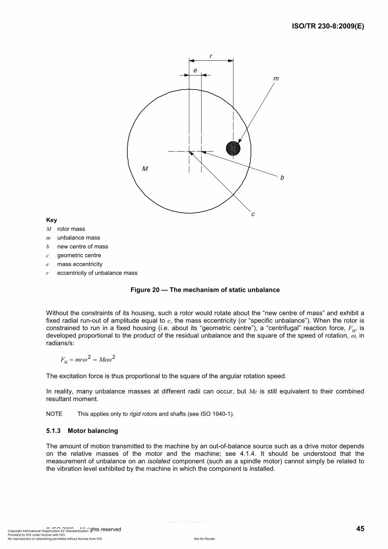
ISO/TR 230-8:2009(E)


Key M rotor mass m unbalance mass b new centre of mass c geometric centre e mass eccentricity r eccentricity of unbalance mass

Figure 20 — The mechanism of static unbalance

Without the constraints of its housing, such a rotor would rotate about the “new centre of mass” and exhibit a fixed radial run-out of amplitude equal to e, the mass eccentricity (or “specific unbalance”). When the rotor is constrained to run in a fixed housing (i.e. about its “geometric centre”), a “centrifugal” reaction force, Fu, is developed proportional to the product of the residual unbalance and the square of the speed of rotation, ω, in radians/s:

2 2uF mr Meω ω= =

The excitation force is thus proportional to the square of the angular rotation speed.

In reality, many unbalance masses at different radii can occur, but Me is still equivalent to their combined resultant moment.

NOTE This applies only to rigid rotors and shafts (see ISO 1940-1).

5.1.3 Motor balancing

The amount of motion transmitted to the machine by an out-of-balance source such as a drive motor depends on the relative masses of the motor and the machine; see 4.1.4. It should be understood that the measurement of unbalance on an isolated component (such as a spindle motor) cannot simply be related to the vibration level exhibited by the machine in which the component is installed.



--`,,```,,,,````-`-`,,`,,`,`,,`---

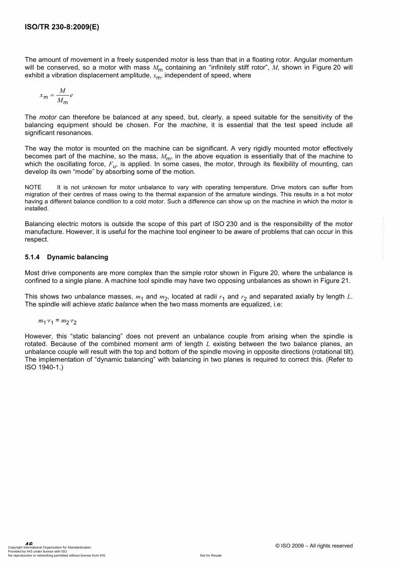
ISO/TR 230-8:2009(E)


The amount of movement in a freely suspended motor is less than that in a floating rotor. Angular momentum will be conserved, so a motor with mass Mm containing an “infinitely stiff rotor”, M, shown in Figure 20 will exhibit a vibration displacement amplitude, xm, independent of speed, where

mm

Mx eM

=

The motor can therefore be balanced at any speed, but, clearly, a speed suitable for the sensitivity of the balancing equipment should be chosen. For the machine, it is essential that the test speed include all significant resonances.

The way the motor is mounted on the machine can be significant. A very rigidly mounted motor effectively becomes part of the machine, so the mass, Mm, in the above equation is essentially that of the machine to which the oscillating force, Fu, is applied. In some cases, the motor, through its flexibility of mounting, can develop its own “mode” by absorbing some of the motion.

NOTE It is not unknown for motor unbalance to vary with operating temperature. Drive motors can suffer from migration of their centres of mass owing to the thermal expansion of the armature windings. This results in a hot motor having a different balance condition to a cold motor. Such a difference can show up on the machine in which the motor is installed.

Balancing electric motors is outside the scope of this part of ISO 230 and is the responsibility of the motor manufacture. However, it is useful for the machine tool engineer to be aware of problems that can occur in this respect.

5.1.4 Dynamic balancing

Most drive components are more complex than the simple rotor shown in Figure 20, where the unbalance is confined to a single plane. A machine tool spindle may have two opposing unbalances as shown in Figure 21.

This shows two unbalance masses, m1 and m2, located at radii r1 and r2 and separated axially by length L. The spindle will achieve static balance when the two mass moments are equalized, i.e:

m1·r1 = m2·r2

However, this “static balancing” does not prevent an unbalance couple from arising when the spindle is rotated. Because of the combined moment arm of length L existing between the two balance planes, an unbalance couple will result with the top and bottom of the spindle moving in opposite directions (rotational tilt). The implementation of “dynamic balancing” with balancing in two planes is required to correct this. (Refer to ISO 1940-1.)



--`,,```,,,,````-`-`,,`,,`,`,,`---

ISO/TR 230-8:2009(E)


Key m1 unbalance mass 1 at radius r1 m2 unbalance mass 2 at radius r2

NOTE For static balance m1·r1 = m2·r2.

Figure 21 — Spindle with dynamic unbalance

5.1.4.1 Drive components

Additional rotating elements within the drive train may also give rise to unbalance effects. With intermediate shafts rotating at different speeds, the opportunity arises for the excitation of a number of different resonances simultaneously. For one-to-one ratios, the balance will be affected by the type of drive. Timing belts (and gears) give fixed-phase relationships, and the resultant balance may well depend on this. Sometimes, however, the situation can be exploited so that, by adjusting the relative tooth positions, it is possible to optimize the resultant balance. For non-positive drives, such as vee-belts or flat belts, speed ratios will inevitably fluctuate slightly with belt slip, and this can result in beats as the unbalance forces go into and out of phase.

5.1.5 Transmission of unbalance forces; units of unbalance

As shown in 5.1.2, the excitation force is proportional to the square of the speed of rotation. It is the machine’s response to this force that gives rise to the perceived vibration.

The unbalance force is a rotating vector and can therefore excite modes in any direction within the plane of its rotation. Thus, the unbalance of the spindle shown in Figure 26 (see 7.1.2) can excite both an X direction and a Y direction mode with, of course, a 90° phase difference between the two.

The units used for measuring or quoting unbalance sometimes give rise to confusion. To redress this, in the following paragraph, the transmission of vibration in the machine tool from an unbalanced rotor is recapitulated with relevant SI units shown between parentheses.



--`,,```,,,,````-`-`,,`,,`,`,,`---

ISO/TR 230-8:2009(E)


Initially, the unbalance is a mass-moment quantity, determined by the product of mass and distance (kg·mm). This is sometimes expressed as a simple length (mm), being the eccentricity of the rotor caused by the unbalance (or “specific unbalance”). (The assumed missing “mass” is the total mass of the rotor.) A freely floating rotor will exhibit a run-out of displacement amplitude equal to its mass eccentricity (mm). Forcing the rotor to run in fixed journals converts this displacement amplitude into a force (N), derived through the mass and rotational velocity of the rotor. The resultant (“centrifugal”) force transmitted causes the machine to vibrate according to its dynamic stiffness at a frequency matching the speed of rotation. So, although the vibration of the machine (i.e. its displacement response) can be measured in millimetres, there is no direct connection between this millimetre measurement and the specific unbalance, also measured in millimetres.

NOTE The vibration displacement amplitude or run-out of a freely supported motor is constant and does not vary with speed. The equivalent force that develops is, however, proportional to the square of the speed, and the displacement amplitude of the machine then follows the response shown in Figure 10.

5.2 Vibrations occurring through the operation of linear slides

5.2.1 General

This clause is concerned with the effect that rapidly accelerating or decelerating feed motion slides can have on machining performance, particularly surface finish. The rapid acceleration of a massive slide can generate a reaction impulse in any direction within the structure, generally exciting the lower modes of vibration. Both linear and rotational vibrations (mainly tilt motions) can occur. These can persist for many seconds because of their slow rate of natural decay. If this occurs during machining, deterioration of the surface finish results from relative vibration between tool and workpiece. (This effect can occur in a direction different from the one providing the impulse through “cross response” effects.)

This phenomenon can be observed by carrying out supplementary “dynamic” straightness tests between the tool side and the workpiece side of the machine. Alternatively, relative (displacement) measurements, orthogonal to the direction of motion, between the tool side and the workpiece side of the machine can be carried out. Suitable tests for these are described in 7.2.

5.2.2 Problems with low-frequency modes

Although the effects of such vibration are manifested in the relative movement between tool and workpiece, it can happen that the particular mode excited may go unnoticed by a frequency response test carried out at this location. The impulse effect of machine slides accelerating will excite the lowest modes because these are the weakest. But these low frequencies also have a long decay time, which can then make them troublesome. This means that quite a small relative movement between tool and workpiece can persist for several seconds, sufficient to produce visible marking of the workpiece. Such modes can be missed on a frequency response test because, at the usual excitation location, they possess relatively high dynamic stiffnesses and the resultant displacement amplitudes are therefore quite small. The location of the impulse from the slide acceleration is not necessarily between the tool and workpiece, however, and can occur wherever the dynamic stiffness is much lower. Normally, this would suggest that such a vibration should have little influence at the tool point, but, because of the low frequency (and hence low damping), it can become troublesome by its persistence after the disturbing impulse has ceased.

5.2.3 Inertial cross-talk

A systematic effect can be observed whenever a significant offset exists between the centre of mass of a driven machine element (e.g. a moving table) and the feed driving force. Tilt motions during accelerations and decelerations lead to displacements of the tool centre point (TCP) perpendicular to the direction of the nominal movement. The factors influencing these lateral displacements are the acceleration force, the offset between the centre of mass and the driving force, the rotational stiffness of the guide-way carrying the table and the axial distance between the centre of mass and the TCP.

Figure 22 shows this effect, known as inertial cross-talk. The offset drive force creates a moment, which generates a rotational displacement dependent on the rotational compliance of the underlying guide-way system, g. This rotational motion transforms geometrically into a lateral displacement of the TCP proportional to the axial offset of the TCP to the centre of mass, M. This is shown in Equation (26).



--`,,```,,,,````-`-`,,`,,`,`,,`---

ISO/TR 230-8:2009(E)


Key M moving mass of the slide g guide-way system TCP tool centre point

Figure 22 — Inertial cross-talk

In Figure 22, EYZ is the straightness deviation due to inertia forces; Fa is the acceleration force (mass to be moved M × acceleration a); ∆YFa is the offset between the centre of mass and the driving force; ∆ZTCP is the distance between the centre of mass, S, and the TCP; and kY1 and kY2 are representative stiffnesses in the y direction located in the z direction at ∆Zk1 and ∆Zk2 respectively.

a Fa TCP Fa TCP2rot,A Y,i i A,j

Y Z Y Z... (26)

zi j

F MaEYZ

k k k

∆ ∆ ∆ ∆= =

∆ +∑ ∑

NOTE krot,A is the rotational stiffness of the underlying structure (e.g. guide-way) given by the individual stiffnesses in the y direction, kY, taking into account their locations in the z direction and the rotational stiffnesses, kA, around the X axis.

Technical Box 9 — Effects of inertial cross-talk

For the evaluation of these cross-talk effects on a machine tool, the influence of a limited change of acceleration with respect to time (jerk) is noticeable. At low feed rates, the nominal acceleration value occurring at high feed rates is not reached and therefore the maximal values of the measured cross-talk effects are reduced.

Owing to the low-pass behaviour of the machine tool, these effects are reduced when acceleration times are short.

5.3 Vibrations occurring externally to the machine

5.3.1 General remarks

The remarks in this subclause are applicable to installed machines only.

The supporting surface on which the subject machine is mounted may have motion induced in it as a result of external forces from other machinery in the surrounding area. This motion can be either periodic, impulsive or a mixture of both. The transmission of such motion to the machine can have a degrading effect on the accuracy and performance of the machine.



--`,,```,,,,````-`-`,,`,,`,`,,`---

ISO/TR 230-8:2009(E)


Externally generated vibrations of this kind are generally beyond the control of the manufacturer (aside from his responsibility to provide guidance on the provision of suitable foundations). The need for a test to evaluate the effects of extraneous vibrations on an installed machine can be driven by a number of quite disparate requirements, such as:

⎯ determination of the overall environmental vibration;

⎯ analysis, identification and suppression of an external source of vibration disturbance;

⎯ elimination of spurious external signals from structural analyses.

See also the discussion on “transmissibility” in 4.5.4 and on machine location in 6.9.

5.3.2 External sources

Sources of external vibration can be other machine tools in the same or a neighbouring workshop. They may also be located much further afield, for example:

⎯ factory equipment such as heavy-duty air compressors. These have been known to set up standing waves in the floor, in which case the careful positioning of the machine tool at a nodal point can almost eliminate this effect. Travelling waves are clearly more problematic;

⎯ nearby rail traffic. This can be particularly troublesome because of the persistent regular low-frequency beat, particularly when rail gaps are present;

⎯ passing road traffic (not usually a problem);

⎯ the breaking of waves on a nearby seashore. This has been known to cause machine tool vibration problems and has been diagnosed by noticing the pattern shifting with the times of the tides.

Grinding machines can be particularly sensitive to low-frequency extraneous vibrations.

5.4 Vibrations initiated by the machining process: forced vibration and chatter

5.4.1 Machining performance limitations

The machining process inevitably generates a considerable amount of vibration, which is reflected in a less-than-perfect surface finish. As the metal removal rate is increased and the cutting force increases, the vibration and the resulting deterioration in the machined surface increase commensurately. The surface roughness may well increase beyond an acceptable level before the maximum rated power is reached for the type of machine. In this case, the machine’s performance is deemed to have been limited by the value of forced vibration occurring through the machining process. For example, in a milling operation, vibration often occurs at the frequency of the tooth impact on the workpiece, which in turn excites the machine. This is especially detrimental when the impact frequency corresponds to a natural frequency of the machine or to one of its harmonics.

5.4.2 Self-excited vibrations (chatter)

Sometimes, a small increase in metal removal rate can lead to a sudden and disproportionate deterioration in surface finish with an accompanying marked increase in noise and vibration. This is recognized as chatter. The onset of chatter in a machining process depends on the cutting parameters, the workpiece material and the method of support, the type of tooling and the dynamic stiffness of the machine’s overall structure, and, especially, the relative orientation of the cutting force with respect to the direction of the natural vibration modes of the machine tool. A self-excited vibration generally occurs in the neighbourhood of a natural frequency (see also 5.4.3). In this respect, an indication of the likelihood of susceptibility to chatter is given when the maximum negative real part of the transfer function exceeds unity. See also the comments in 4.4.4 on “Nyquist” stability and the significance of maximum negative real parts (see 4.4.3).



--`,,```,,,,````-`-`,,`,,`,`,,`---

ISO/TR 230-8:2009(E)


A number of different physical mechanisms have been identified by researchers to account for the generation of chatter, but which one actually occurs depends on the type of cutting process employed and the structure of the machine. The mechanisms explaining milling and turning operations, for example, are often quite different. Figure 23 illustrates how regenerative vibration (or chatter) can build up from a single point turning operation where the undulating surface of previously cut material provides positive feedback to the cutting force. The regenerative loop effectively results in negative equivalent damping (see 4.7.4.3).

The discussion of other possible chatter “mechanisms” is, however, beyond the scope of this part of ISO 230. But it should be noted that, for any fixed set of conditions, chatter will usually occur (if it occurs at all) when a certain threshold of metal removal rate is exceeded. In particular, the spindle speed is often a critical parameter. The stability diagram, expressing the chatter-free cutting depth against rotational spindle speed often shows successive stable and unstable domains known as “instability lobes” — see Figure 24.

Avoidance of chatter is best achieved through good machine design. High static stiffness and low mass in the critical components should always be sought. The addition of vibration absorbers (see 4.6.2) can often be beneficial. It should be noted that “good machine design” might not always be sufficient. A “structural weakness” promoting chatter can exist in the workpiece itself or in its means of support (e.g. fixturing).

Fdist F xd

µTt+kcbb

-

t1 t2 t3 t4Fdist F F F F

xd xd m

xd

k

c

Gg(jω)M)

P) Key P) process b width of cut kcb specific cutting force Tt dead interval µ overlap factor

M) machine Gg( jω) relative frequency

response function

t1, t2, time steps t3, t4 F force excitation Fdist disturbing force xd machine displacement amplitudem mass k stiffness c damping

Figure 23 — Regenerative chatter process showing position of vectors, excitation force, F, and machine deformation, xd, for directional compliance characteristic, Gg( jω)



--`,,```,,,,````-`-`,,`,,`,`,,`---

ISO/TR 230-8:2009(E)


Key S spindle speed (r/min) d axial depth of cut (mm) ST stable region UST unstable region

Figure 24 — Chatter stability lobes showing regions of stability and instability

5.4.3 Forced vibration versus chatter

The cutting process is an important source of forced vibration even without chatter developing. Forced vibration per se should be clearly distinguished from chatter. Forced vibration occurs at the excitation (i.e. cutting) frequency, which can be determined by the number of cutting edge impacts per second19), and increases more or less linearly with the metal removal rate. Chatter occurs non-linearly, often increasing dramatically following the initial trigger. It is fuelled by regenerative feedback and is therefore generally close to one of the machine’s natural frequencies. If the natural frequency happens to lie near to the cutting frequency or one of its harmonics, then the machine’s resistance to chatter will be very much reduced.

5.5 Other sources of excitation

The previous subclauses have examined the particular sources of vibration specified in the scope of this part of ISO 230. Some other important sources of vibration, which could have a deleterious effect on surface finish and produce palpable vibration are:

⎯ unstable servo systems for feed and spindle drives;

⎯ gears and belt drives;

⎯ the effect of worn bearings;

⎯ the cycling of ancillary equipment such as tool changers and pallet changers.

19) This description is specific to the milling process only.



--`,,```,,,,````-`-`,,`,,`,`,,`---

ISO/TR 230-8:2009(E)


More than brief mentions of the mechanisms of such sources are outside the scope of this part of ISO 230. Nevertheless, much of the general background information provided will still be pertinent, particularly with regard to the identification of frequencies and levels.

5.5.1 Unstable servo systems

The underlying mathematics for servo sytems are similar to that for structural vibrations and, although damping is generally much higher, it is still possible to generate resonances when high “gains” are employed. These will, in turn, excite the machine structure — though not necessarily between tool and workpiece — and, if these resonances are sufficiently close to a structural resonance, they can become quite problematic. Clearly, analysis of servo systems is a specialized subject beyond the scope of this part of ISO 230.

5.5.2 Gears and belt drives

Gear drives are an important source of both vibration and noise. Vibration is generated between a pair of meshing gears because of so-called “transmission errors” resulting from a less-than-perfect involute20) form for the profiles of the gear teeth. These errors inevitably increase as the teeth deform under heavy loads. Transmission errors indicate that the constant rotational velocity of a driving gear is not faithfully transmitted to the driven gear. Additionally, a series of small torsional impulses is generated each time a pair of teeth comes into contact, the size of the impulse increasing with both load and speed. (The effect is mitigated by using helical gears, which permit a gradual take-up of the load by the teeth.)

The train of impulses generated by the rotation of the gear manifests itself as a complex wave whose fundamental frequency is equal to the tooth impact frequency (number of teeth × rotational speed). Because of its complexity, this wave (created by impulses) will be rich in harmonics. A frequency analysis will reveal the meshing frequency with perhaps six or more harmonics, plus another characteristic of gear vibration: a family of “side-bands”. Side-bands are smaller peaks at frequencies spaced around the meshing frequencies. The spacing is determined by the rotational frequency of the individual gear and provides a diagnostic tool for picking out which of a meshing pair is faulty. See the example in Technical Box 10.

Generation of vibration from toothed belts can also occur at tooth contact frequency. Usually, however, the low stiffness of the belt means that the forces generated are minimal. Furthermore, the entrapment of air can create a corresponding noise problem out of all proportion with the structural vibration produced. Frequencies other than that of the rate of tooth contact can also occur, such as the bending frequencies of individual teeth.

5.5.3 Worn bearings

The generation of vibration and noise from worn or faulty bearings is well documented in the literature on condition monitoring (see for example ISO 13373-2). Vibration velocity is generally proportional to the rotational speed, but the frequencies generated are more complicated and depend on relative dimensions of rotating elements and their rates of precession, and also whether a fault lies in an outer race, an inner race or one or more of the rolling elements. Excessively worn bearings can also generate self-excited vibrations through shaft-whirl and dry friction.

5.5.4 Ancillary equipment

Tool changers and pallet changers can give rise to impulses as they lock into place. The effect on a machine tool is similar to slide acceleration effects, and similar techniques should be used to evaluate such problems.

Other types of ancillary equipment might be equipped with rotating members having the propensity for generating out-of-balance forces. Again, the tests on spindle unbalance are applicable here. A spectral analysis of such equipment will highlight unbalance as a peak at the rotational frequency.

20) This is the geometric shape of a tooth face that ideally allows for a pure rolling action between the mating profiles and hence permits a perfectly smooth (and vibration-free) transmission. However, even a perfect involute will deform as soon as it starts to transmit a load.



--`,,```,,,,````-`-`,,`,,`,`,,`---

ISO/TR 230-8:2009(E)


Consider a 40 tooth gear running at 600 rpm meshing with a 50 tooth gear:

Rotation speed of first gear = 600 rpm = 10 Hz

Rotation speed of second gear = 600 × 40/50 = 480 rpm = 8 Hz

Tooth impact frequency = 40 × 600/60 = 50 × 480/60 = 400 Hz

A frequency response test would reveal a peak at 400 Hz and probably also the harmonics at 800 Hz and 1 200 Hz. Note that, although this is the fundamental tooth impact frequency, it is also the 40th and 50th harmonic of the two rotational frequencies. Side-bands for the first gear would show as, say, the 38th, 39th, 41st and 42nd harmonics, viz. at 380 Hz, 390 Hz, 410 Hz and 420 Hz, i.e. spaced at the rotational frequency of 10 Hz. Side-bands for the second gear would show as the 48th, 49th, 51st and 52nd harmonics of its rotational frequency of 8 Hz, viz. at 384 Hz, 392 Hz, 408 Hz and 416 Hz. These families of side-bands can very easily be identified from frequency spectrum analysis plots and the culprit gear thereby pinpointed.

Side-bands are generated through amplitude and frequency modulation effects owing to inherent errors in concentricity between the pitch circle and the centre of rotation. Families of side-bands can be seen accompanying some of the harmonics too.

NOTE The technique of identifying gears fails when the ratio is 1:1. It is also similarly unreliable for simple ratios such as 2:1, 3:1, etc.

Technical Box 10 — Vibration frequencies of meshing gears

6 Practical testing: general concepts

6.1 General

Practical dynamic testing of machine tools generally includes the following points:

⎯ Testing the machine at rest, fixed on its support. This should include the determination of the vibration values, the natural frequencies, the modal shapes of the machine at these frequencies and, if possible, the chatter susceptibility.

⎯ Testing the machine unloaded while the different elements are rotating or moving, in order to investigate sources of vibration.

⎯ Testing the machine working under load to determine the cutting performance, chatter susceptibility and the quality of the finished piece (including dimensional accuracy, surface quality, etc.).

A complete dynamic testing programme for a machine tool can take days and is therefore very expensive. In this clause, a number of tests are briefly described, but this is by no means an exhaustive list. The machine tool builder and the customer should reach a preliminary agreement on the programme of tests to be performed and choose the most appropriate ones considering the type of work to be executed on the machine, as well as the requirements to be met.

The tests described below are based on the practice of experts and are not intended to be imposed as a standard procedure.

6.2 Measurement of vibration values

The measurement of vibration is essentially the measurement of a waveform, the amplitude of which may vary in a predictable, periodic way or may be entirely random. For accurate measurement, it is necessary to employ calibrated transducers capable of reproducing a representation of the waveform over the frequency range of interest, and also to take account of any deflection of the transducers.

Further processing is required to analyse the waveform of the vibration signal (either by digital or analogue means) and characterize it into a set of meaningful parameters. The simplest method is to compute the mean power value of the signal without any reference to its frequency content. This is essentially a “broadband” measurement.



--`,,```,,,,````-`-`,,`,,`,`,,`---

ISO/TR 230-8:2009(E)


More complex processing allows the frequency range to be divided into a series of narrow bands, where the power in each band can be measured. As the bandwidths become narrower, the processing time will increase 21).

6.3 Instrumentation

6.3.1 General

The instrumentation used should be designed to operate satisfactorily in the environment for which it is to be used with respect to temperature, humidity, etc.

Calibrated transducers are available for the direct measurement of displacement, velocity and acceleration amplitudes. Most types of transducer require additional equipment for further signal processing. Absolute displacement and velocity transducers are designed to be used above their own natural frequencies. Consequently, their seismic masses are generally quite high and can directly influence the measurement. Accelerometers operate below their own natural frequency and therefore have low masses. For general vibration work on machine tools, piezo-type accelerometers are preferred, though capacitive and eddy-current displacement transducers are also available and are often quite useful.

The method for mounting accelerometers is covered by ISO 5348:1998, and particular reference should be made to 4.4. Shear-type transducers, as opposed to compression-type, are recommended since they are less sensitive to temperature variations and damp environments. (ISO 2954 covers the requirements of instruments for measuring vibration severity, but is currently limited to velocity transducers.)

Conversion between displacement, velocity and acceleration requires integration or differentiation as described in Annex B. (Displacement from an accelerometer needs a double integration.) For analogue systems, this can be carried out using passive electrical networks. For digital systems, direct numerical integration and differentiation is possible, though care shall be taken to ensure that the integrity of phase relationships is preserved.

For most machine tool work, the mass of the vibration transducer is usually insufficient to influence the measurement significantly, particularly when accelerometers are used. However, for lightweight structures or lightweight elements of a structure, this may not always be so. An indication of whether the mass of the transducer is too great can be obtained by doubling its mass (e.g. by adding an equivalent dummy mass) and checking the change in vibration reading. The vibration amplitude should not change by more than 12 %, as per ISO 2954. A similar check should also be made to ensure that the transducer does not significantly influence the natural frequency by more than 5 %.

Laser-based vibration measurement systems (e.g. laser vibrometers) are also available, some of which can directly measure dynamic displacement, and then use differentiation to obtain velocity and acceleration data. Some of these systems can also measure differentially to determine the relative vibration of the tool-holding part with respect to the workpiece-holding part of the machine.

6.3.2 Broadband measurements

Two instrument systems presently in common use for monitoring broadband vibration in the evaluation of unbalance and environmental vibration are:

⎯ instruments that incorporate RMS detector circuits and display RMS values;

⎯ instruments that incorporate either RMS or averaging detector circuits, but are scaled to read peak-to-peak or peak values. The scaling is based on an assumed sinusoidal relationship between RMS, average, peak-to peak and peak values. (For details of these relationships, see Annex B.)

21) Depending on the type of instrumentation employed.



--`,,```,,,,````-`-`,,`,,`,`,,`---

ISO/TR 230-8:2009(E)


This type of equipment is suitable for general vibration measurement such as velocity measurements from unbalanced spindles — particularly for the grade test described in 7.1.5.1.

6.3.3 Narrow-band measurements

Spectrum analysis of both noise and vibration signals requires additional equipment, and, for the measurement of frequency response, this should provide an excitation signal enabling the transfer function between input and output to be measured. Basic requirements include a dynamic signal analyser, a vibration exciter and a force transducer. Sophisticated systems are now available for carrying out a full compliance analysis including modal shapes.

Without such equipment, it is still possible to determine approximate mode shapes using a twin-beam oscilloscope and hand-held probes.

6.4 Relative and absolute measurements

Relative vibrations are measured between two locations (e.g. tool and workpiece) using a suitable transducer attached through a movable member to both locations. In Figure 25 (left-hand view), both excitation and measurement are relative and occur between the tool and workpiece. In the right-hand view, they are both absolute and measurement can thus be made at any point on the structure. Generally, it will be more satisfactory to use a representative dummy tool and workpiece at the tool and workpiece locations rather than to use real components. Absolute vibrations are measured with inertial devices at a single point. The difference in values from the two types of measurement depends on the relative phase of the vibration at the two locations. Note that measuring relative vibration gives a better estimate of the true vibration severity. Summing the absolute vibrations at both locations gives the “worst-case” value and may be an acceptable alternative to measuring relative vibration. Where the absolute vibration at one location is very much smaller than at the other, it is sufficient to quote the single (i.e. “worst”) value.

A method of obtaining relative displacement amplitudes from absolute values for a cylindrical grinding machine is given in Annex E (Example 1).

An exciter when used “absolutely” can occupy an external mounting position (as shown in Figure 25, right-hand view), but note that the force transmitted does not depend on the mounting: like a space rocket, the exciter does not need anything physical to “push against”. However, the performance of a small exciter of low mass may be hampered if it is not physically supported, because the displacement amplitude of its body reaction (see 4.1.4) may increase so much that the plunger travel becomes constrained by the end stops with consequential clipping of the signal and distortion of the output. Note that using the exciter against an external reference point means that fundamental low-frequency rocking modes of the machine on its foundations can now be examined. The relative method of excitation shown on the left will generally not excite these modes. Note the influence of a static preload on the excitation described in Figure 25, and see 8.4 for further comments on this topic.

6.5 Units and parameters

Vibrations may be quantified by any of the following parameters:

⎯ vibration displacement, measured in micrometres (µm);

⎯ vibration velocity, measured in millimetres per second (mm/s);

⎯ vibration acceleration, measured in millimetres (or metres) per second squared (mm/s2 or m/s2), or g (1g ≈ 9,81 m/s2).



--`,,```,,,,````-`-`,,`,,`,`,,`---

ISO/TR 230-8:2009(E)


Fstat = 0,2 - 5 kNx

F Fstat dyn+

Fdyn

Fdyn

F m= x

Key F force Fstat static force Fdyn dynamic force m exciter mass x acceleration

Relative excitation

— electro-hydraulic

— piezo-electric

— electrodynamic

Types of exciter

Absolute excitation

Relative excitation against an external reference point

— impulse hammer

— electro-hydraulic absolute exciter

The static preload eliminates bearing clearance Influence of clearance

No static preload, bearing clearance appears as non-linearity

Figure 25 — Comparison of excitation and measuring methods

The choice of parameter is usually dictated by the application and the type of measuring equipment used. In general, displacement values are preferred, except possibly when dealing with unbalance conditions, where velocity measurements are an acceptable option22). Note that the units being measured by the equipment are not necessarily the same as those required for reporting results.

Note further that when these measurement parameters are related to input force, additional concepts are introduced:

⎯ compliance = displacement per unit force;

⎯ stiffness = force per unit displacement;

⎯ mobility = velocity per unit force;

⎯ accelerance = acceleration per unit force.

22) And also for noise-related problems where vibration velocity more closely parallels sound pressure level.



--`,,```,,,,````-`-`,,`,,`,`,,`---

ISO/TR 230-8:2009(E)


Additional different methods of evaluating these parameters in common use are:

⎯ amplitude or peak (0-p);

⎯ peak-to-peak (p-p);

⎯ root mean square (rms);

⎯ average.

The use of amplitude measurements is preferred. Again, an exception may be made for measurements of unbalance where it is common practice, when evaluating broadband vibration of rotating machinery in velocity units, to consider the rms value of the velocity, since this can be related to the power of the vibration.

In order to prevent confusion and to ensure the correct interpretation, it is important at all times to identify clearly and completely the measurement units [e.g. µm (peak) or mm/s (rms)] as well as the sensitivity, range of linearity, and measurement uncertainty of the instrument used. (See 6.6.)

For a simple sine-wave vibration, there are established mathematical relationships between measurement parameters and their methods of measurement (see Annex B). Note that, in the general (i.e. non-sinusoidal) case, these relationships become less accurate as the harmonic distortion increases.

6.6 Uncertainty of measurement

There is always a degree of uncertainty associated with vibration measurement. This is often as much to do with the nature of the structure being measured and the environment as with the uncertainty associated with the measuring equipment. This applies particularly to measurements of vibration amplitudes close to resonance, where a small change in frequency can precipitate a large change in amplitude. For a lightly damped structure, these amplitudes are inversely proportional to the degree of damping present, which in turn is susceptible to slight variations in friction level (through wear, lubrication, etc.) and the difficulty of controlling the test conditions — see 4.7.4. Because of this, and because of the wide range of vibration amplitudes experienced, the use of a logarithmic scale (e.g. noise measured in decibels) can sometimes provide a more realistic way of evaluating vibration; see Figure 30.

In the absence of a logarithmic scale, values of vibration amplitude (whether displacement, velocity or acceleration) need not normally be quoted to a resolution greater than 0,1 % of the maximum value.

Frequency values can usually be determined with more precision than displacement, velocity or acceleration values, and do tend to fluctuate less. The accuracy of a frequency measured with a digital signal analyser is, however, strictly limited by the bandwidth and hence dependent on the frequency range. It also depends on the data acquisition module, the sampling frequency and averaging process used with the measurement data along with the type of digital signal analyser used. For most machine tool vibration work, as presented in this document, frequencies should be accurate to about 2 Hz (or about 0,3 % of the measurement bandwidth). This should be quite adequate for most investigations.

If the frequency analysis equipment has facilities for carrying out a coherence test (see 8.2), this will provide a certain degree of confidence in the veracity of the frequency response.

The use of such vibration analysis equipment demands a certain level of knowledge, experience and proficiency on the part of the user who should take time to become familiar with the general operating principles of the equipment. In particular, care should be taken against generating spurious results, such as aliasing, through the inappropriate use of the equipment.

6.7 Note on environmental vibration evaluation

Vibration at the spindle nose can also arise from other sources of forced vibration within the machine or even from sources external to the machine. For these, the velocity and frequency of vibration will be independent of the spindle speed. For the tests described in this document, it is not necessary to determine these other sources of vibration, although they can usually be located by starting up the machine components one by one.



--`,,```,,,,````-`-`,,`,,`,`,,`---

ISO/TR 230-8:2009(E)


However, if the measured vibration amplitude exceeds a particular recommended limit, it will then be necessary to take supplementary measurements of the environmental vibration, as described in 7.3. This should be carried out with the machine shut down to ensure that external vibration is not making a significant contribution to the observed vibration. Where possible, steps should be taken to reduce the magnitude of environmental vibration if it is greater than one-third of the recommended limit for the machine.

6.8 Type testing

In cases where the degree of excitation of vibration varies little between individual machines of the same type, it is sufficient to test a single machine as being representative of its type.

Generally, vibration generated either through the machining process or through the acceleration of machine slides relates to the overall structure and design of the machine tool, and thus falls into this category. Similarly, the investigation of modes and natural frequencies can be accomplished by type testing.

Spindle drive unbalance, however, is usually the result of small manufacturing imperfections, which can vary from machine to machine. Consequently, this type of vibration cannot be satisfactorily represented by a single type test, and individual testing therefore becomes necessary. A type test may, however, be carried out to check whether the effects of unbalance are significant in each measurement direction. Similarly, the existence of externally generated forced vibration is usually unique to the installation, and thus also requires an individual test.

It should be noted, however, that the foundation can significantly influence the behaviour of individual machines and it is therefore wise to avoid this influence when individual machines are being compared.

6.9 Location of machine

The machine tool should be correctly installed on a suitable foundation approved by the manufacturer. If the machine is mounted on individual isolation mounts, the type and specification of such mounts should be recorded for each test. See notes on transmissibility to and from floors in 4.5.4 and Figure 11.

Generally, securing the machine to a massive foundation is the best procedure for minimizing most types of vibration. (And, of course, the machine may be designed with this in mind, i.e. the floor might be intended to form part of the structure.) An exception arises, however, when the floor is transmitting vibration from an external source and the frequency is close to a machine mode. It can sometimes be beneficial to employ damped isolating supports as shown in Table 2, but this depends on the frequency being transmitted.

Table 2 — Effect of amount of damping on isolation mountings

Frequency of transmitted vibration

Machine fixed rigidly to foundation

Optimum type of support Result of using optimum type of support

Far below machine resonance

Machine moves with floor Little to choose from No reduction in transmitted vibration

Close to resonance Machine greatly amplifies floor movement

High level of damping Slight increase in transmitted vibration

Far above resonance Machine moves very little Low level of damping best Large reduction in transmitted vibration

It should be understood that the use of “soft” isolation mounts to minimize transmissibility might aggravate the response of the machine to vibrations occurring internally.

It is recognized that, for tests carried out in manufacturers' plants, it may not always be possible to install machines as described above, and that the accuracy of subsequent vibration tests could then be jeopardized. In particular, the reaction to high acceleration rates of heavy slides could cause poorly secured machines to move laterally on the floor. (See 7.2.1.)



--`,,```,,,,````-`-`,,`,,`,`,,`---

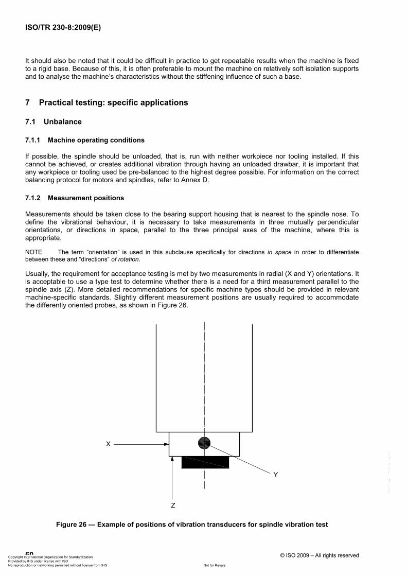
ISO/TR 230-8:2009(E)


It should also be noted that it could be difficult in practice to get repeatable results when the machine is fixed to a rigid base. Because of this, it is often preferable to mount the machine on relatively soft isolation supports and to analyse the machine’s characteristics without the stiffening influence of such a base.

7 Practical testing: specific applications

7.1 Unbalance

7.1.1 Machine operating conditions

If possible, the spindle should be unloaded, that is, run with neither workpiece nor tooling installed. If this cannot be achieved, or creates additional vibration through having an unloaded drawbar, it is important that any workpiece or tooling used be pre-balanced to the highest degree possible. For information on the correct balancing protocol for motors and spindles, refer to Annex D.

7.1.2 Measurement positions

Measurements should be taken close to the bearing support housing that is nearest to the spindle nose. To define the vibrational behaviour, it is necessary to take measurements in three mutually perpendicular orientations, or directions in space, parallel to the three principal axes of the machine, where this is appropriate.

NOTE The term “orientation” is used in this subclause specifically for directions in space in order to differentiate between these and “directions” of rotation.

Usually, the requirement for acceptance testing is met by two measurements in radial (X and Y) orientations. It is acceptable to use a type test to determine whether there is a need for a third measurement parallel to the spindle axis (Z). More detailed recommendations for specific machine types should be provided in relevant machine-specific standards. Slightly different measurement positions are usually required to accommodate the differently oriented probes, as shown in Figure 26.

Figure 26 — Example of positions of vibration transducers for spindle vibration test



--`,,```,,,,````-`-`,,`,,`,`,,`---

ISO/TR 230-8:2009(E)


7.1.3 Test procedure (grade test and engineering test)

Alternative procedures are offered: a grade test and an engineering test. The grade test is a simple test that enables the machine’s unbalance to be checked quickly for compliance with a prescribed balance quality grade. The engineering method enables a more accurate and detailed assessment of the machine’s unbalance to be made. Although the test procedures are similar, there is a difference in the type of instrumentation employed and in the method of presentation of the results. The selection of the requisite test procedure will depend on the needs of the user.

It should be recognized that because of bandwidth differences, the grade test will give generally higher readings than the more accurate engineering test. Vibrational energy that is not associated with the unbalance condition may also become included. See 4.8.2 for a discussion on the effects of bandwidth.

NOTE The table of grades specified in ISO 1940-1 show that machine tools are normally covered by grades G1 to G6,3 inclusive, though, for high-speed machines, the grade range may need to be extended. It is important to understand that the grades in ISO 1940-1 represent suitable performance values for rigid rotors that may be included in the machine and not the machine itself. It has been shown that the vibration performance of a machine subjected to out-of-balance forces from a rigid rotor is very much dependent on the compliance of the machine, and that the machine itself cannot be considered a rigid system. Although the principle of applying grades to machines has been successfully borrowed from ISO 1940-1, this does not in any way assume that a numerical relationship can be established with the grades presented therein.

The correct protocol for balancing motor and pulley sets or machine tool spindles is described in Annex D.

Measurements shall be made and recorded at the maximum speed of the spindle and at the speed where the velocity (grade test) or the displacement (engineering test) of the vibration is at a maximum. For a machine with distinct spindle speeds, it is necessary to take measurements at each speed in turn in order to determine the maximum value. For a CNC machine tool, where this is practicable, the spindle speed could be programmed to start at top speed. The speed is then progressively decreased in small steps (e.g. 0,5 %) with a short dwell (e.g. 0,3 s), in order to achieve a controlled smooth deceleration until the speed is 1/3 of the maximum 23). Speed is increased again by the same amount until top speed is reached once more. The vibration displacement amplitude value should be continuously monitored during this time. The maximum value should be noted for both the acceleration and deceleration phases, and the speed(s) at which the maximum value occurs should also be noted. This should subsequently be confirmed by checking during continuous running at the speed(s) concerned.

A type test should be carried out to check whether the direction of rotation is significant for this type of machine. If so, and the machine spindle is designed to run in either direction, then the test should be carried out for both directions of rotation.

For machines with multiple independently driven spindles, it will be necessary to repeat the test for each spindle.

7.1.4 Specific notes on instrumentation

7.1.4.1 Grade test instrumentation

Instrumentation for this test can consist of an integral hand-held meter or a velocity transducer and associated measuring equipment. For establishing grades, it is important to be aware that instruments may not be calibrated in velocity amplitude units. Instrumentation of this type usually responds to RMS velocity, which is then converted for display purposes to peak values. These conversions are presented in Annex B, but suffer from some loss of accuracy when signals are non-sinusoidal.

The use of hand-held meters is not recommended for frequencies above 500 Hz.

23) While this minimum test speed is generally suitable, in certain cases, machine specific standards may specify lower values.



--`,,```,,,,````-`-`,,`,,`,`,,`---

ISO/TR 230-8:2009(E)


7.1.4.2 Engineering test instrumentation

Measurement of vibration displacement (or velocity or acceleration) is carried out using calibrated transducers as described in 6.3.

7.1.5 Presentation of results

The information should be presented according to the type of test carried out, as indicated below. See also Example 4 in Annex E.

7.1.5.1 Grade test presentation

This employs the format laid down in ISO 1940-1 where balance grades for rigid 24) rotors are established according to the value of vibration velocity measured. Grades of unbalance for rotating components within specific machines should not exceed the maximum vibration velocities shown in Table 3.

Machine tool rotating components are normally covered by grades G1 to G6,3 inclusive. The notion of a “permissible grade” has been extend here to cover a complete machine, with the permissible grade being determined by agreement between supplier and customer, or by way of machine-specific standards. (See also 7.1.3.) Note that for high-speed spindles, grades higher than shown in Table 3 may be required. Suitable grades for different types of machines should be presented in any relevant machine-specific standards, as should the applicability of the grade test to certain types of machine.

The following information should be supplied:

⎯ maximum “G” grade;

⎯ direction of rotation;

⎯ speed at which maximum vibration velocity occurs;

⎯ location and orientation of transducer;

⎯ orientation of maximum vibration;

⎯ axial positions of all slides;

⎯ details of test equipment;

⎯ details of machine;

⎯ location and date of test;

⎯ environmental conditions of test.

An example of a spindle grade test is given in Annex E (Example 4).

24) See the note in Clause 7.1.3.



--`,,```,,,,````-`-`,,`,,`,`,,`---

ISO/TR 230-8:2009(E)


Table 3 — Balance grades

Balance grade Vibration velocity (amplitude)

mm/s

G0,4 0 to 0,4

G0,63 0 to 0,63

G1 0 to 1,0

G1,6 0 to 1,6

G2,5 0 to 2,5

G4 0 to 4,0

G6,3 0 to 6,3

G10 0 to 10

G16 0 to 16

7.1.5.2 Engineering test presentation

The following information should be recorded for each test:

⎯ direction of rotation;

⎯ vibration values at top speed (two or three orientations). See Notes 1 and 2;

⎯ r/min of top speed;

⎯ maximum vibration value (two or three orientations). See Notes 1 and 2;

⎯ r/min of speed at which maximum vibration value occurs. See Note 1;

⎯ locations and orientations of vibration transducers;

⎯ identification of spindle (if there is more than one);

⎯ axial positions of all slides;




⎯ environmental conditions of test.

This information should be supplemented by graphs of vibration value plotted against spindle speed. See Note 1. See also Example 5 in Annex E.

For high-speed spindles where radial forces are important, it may often be more suitable to use acceleration amplitudes of vibration. Whichever units are used, they should always be stated explicitly; see Note 1.

NOTE 1 The preferred units for this test are vibration displacement amplitudes (peak or RMS), measured in micrometres or millimetres. It is recognized, however, that there are practical situations in the machine tool industry where velocity units may be preferred. Particularly relevant to this is the practice of measuring unbalance in this and other industries, where it is noted that electric motors, being an essential element of a spindle drive system, are often characterized in this way by



--`,,```,,,,````-`-`,,`,,`,`,,`---

ISO/TR 230-8:2009(E)


their manufacturers. For a given degree of unbalance, the measured vibration velocity should generally 25) increase linearly with speed and thus ensure that tighter restrictions are placed on faster machines.

NOTE 2 The number of orientations is determined in 7.1.2.

7.2 Machine slide acceleration along its axis (inertial cross-talk)


If possible, the spindle should be unloaded, that is with neither workpiece nor tooling present. The spindle should be stationary.

It may be necessary to check the influence of workpiece and tooling mass, in which case a second test should be carried out with the machine loaded with masses typical for the machine.

Notwithstanding 6.9, it should be noted that inadequate installation of a machine for testing in this category could result in lateral movement of the machine on the floor as a reaction to the high acceleration of the slides. This can have the effect of reducing the results of the slide acceleration tests because of energy absorption through friction damping (see 4.7.4.2) between the floor and the machine. If this condition prevails, the installation should be considered unsuitable for this test. It also follows, in this case, that this installation would be unsuitable for the machine in service generally.

7.2.2 Measurement positions and instrumentation

Dynamic straightness measurements can be carried out with a cross-grid plate, although a number of other available instruments are suitable.

Relative vibration measurements can be carried out with two absolute vibration transducers aligned in parallel, and the results should be presented in graphical form.

To ensure that vibration of the test equipment (including the fixture) is not influencing the results, it should be checked by frequency analysis (preferably by means of excitation from a small impact). Machine test results occurring at frequencies above the lowest natural frequency found for the test equipment should be discarded.

7.2.3 Test procedure

Straightness measurements should generally be made in accordance with ISO 230-1. They should be carried out both with and without slide acceleration, and measured dynamically, i.e. “on the fly”.

7.2.3.1 Set-up for straightedge

The straightedge should be set up so that the same reading is shown on the displacement transducer for the slide at both its starting and finishing points on the 100 mm travel. If the readout of the displacement transducer is input to a computer, the alignment may be carried out mathematically using suitable software.

A typical set-up is shown in Figure 27. In this example, measurements are being made parallel to, and in line with, the direction of axis feed.

The plot may be either a time graph or an X-Y plot. The locations of the starting and finishing points should also be recorded.

25) That is, at frequencies not influenced by resonances.



--`,,```,,,,````-`-`,,`,,`,`,,`---

ISO/TR 230-8:2009(E)


Key 1 displacement transducers 2 straightedge 3 holding device

a Feed direction.

Figure 27 — Example of set-up using a straightedge

7.2.3.2 Set-up for two-dimensional scale

The two-dimensional scale is set up so that starting and finishing points of the X travel have the same Y coordinate when the slide is at either end-point. The alignment may also be achieved mathematically through software.

A typical set-up for a cross-grid plate on X and Y axes is shown in Figure 28. The measurement procedure is as follows:

a) For each linear feed motion, the tests should be carried out in each of the orthogonal planes over a length of approximately 100 mm in the positive direction at a number of low feed rates (i.e. below 500 mm/min).

b) Test a) should be repeated with acceleration to the maximum programmable (G01) feed rate, followed by a short travel distance and a deceleration to zero. It may be found that a longer length of travel is required when feed rates are high.

c) If possible, a visual comparison of the difference between the measurements in a) and b) should be made and reported.

NOTE Tests can also be carried out at rapid traverse (or maximum feed rate) in order to obtain information on vibration that will mainly influence the wear of components.



--`,,```,,,,````-`-`,,`,,`,`,,`---

ISO/TR 230-8:2009(E)


Key 1 reader head 2 grid plate

Figure 28 — Two-dimensional scale configuration for inertial cross-talk measurements


The results of tests a), b) and c) of 7.2.3.2 should be presented graphically, all to the same scale.

The following minimum supporting information should also be supplied:



⎯ type of equipment used for test;

⎯ name of feed axis under test;

⎯ axial positions of slides not under test;

⎯ direction of measurement of vibration;

⎯ feed rate (mm/min);

⎯ approximate displacement amplitude of vibration during acceleration (mm);

⎯ approximate displacement amplitude of vibration during deceleration (mm).

The settings of any programmable codes that affect slide acceleration should also be recorded, as should the acceleration rate, if known.

An example of the use of a two-dimensional scale for evaluation of this type of vibration is presented in Example 6 in Annex E.



--`,,```,,,,````-`-`,,`,,`,`,,`---

ISO/TR 230-8:2009(E)


7.3 Vibrations occurring externally to the machine


For this test the machine should, if feasible, be completely powered down. If it is suspected that electrical signals are present, the machine should be disconnected from the supply, or the measuring equipment should be electrically isolated from the machine.

7.3.2 Measurement positions

If possible, relative displacement amplitude values between tool and workpiece should be recorded. Since this is not always possible, absolute measurements at both the tool side and the workpiece side are an acceptable alternative, though due recognition of the phase angle should be made and taken into account. See also 6.4.

7.3.3 Test procedure

Vibration values should be recorded over a period of time judged to be representative of the conditions during which the machine would be expected to operate.


When the test is used in isolation, the following information should be presented:

⎯ maximum vibration displacement amplitude, measured in micrometres;

⎯ direction of the maximum vibration;

⎯ duration of test;



⎯ positions of all axes;


⎯ environmental conditions of test;

⎯ description of external operations occurring in the vicinity.

This test may also be used as a supplementary “background” test to other tests (see 6.7), such as those for machine spindle unbalance or for free vibrations induced by accelerating slides. The measurement units used should always be the same as those used in the main test. Where significant background vibration is present, results of this should be presented along with the results of the specific test to which it relates.

For an example of environmental vibration testing, see Examples 2 and 3 in Annex E.

7.4 Vibrations occurring through metal cutting

Because chatter can often be made to occur (or disappear) by the choice of parameters, it is impossible to lay down precise tests for a standardized testing procedure.

To evaluate chatter and/or forced vibration, it is recommended that the machine be set up to carry out a representative machining operation with representative tooling and a “blank” workpiece, selecting the most suitable operating conditions for testing the machine to its full-load rated power. These conditions should always be in accordance with those recommended by the tooling manufacturer.



--`,,```,,,,````-`-`,,`,,`,`,,`---

ISO/TR 230-8:2009(E)


The tester then determines the machine’s limiting criterion for the test with full details of the test being recorded. The test will normally be limited by one of the following primary criteria:

⎯ specified power limit reached without excessive vibration;

⎯ termination of test through excessive forced vibration;

⎯ termination of test through chatter.

The level of acceptability reached by excessive forced vibration or by chatter may be determined by one of the following secondary criteria:

⎯ surface finish;

⎯ workpiece accuracy;

⎯ tool life;

⎯ noise.

Manufacturers following the procedure in this clause should present a set of cutting conditions with the appropriate limiting criteria quoted.

With the aid of spectral analysis equipment, it is possible to determine the frequencies and modes being excited by the chatter phenomenon. It is instructive to analyse both vibration and noise in this respect. Sometimes the chatter is necessarily of short duration and it may then be found expedient to record sound or vibration for subsequent processing.

Normally, the determination of chatter frequency in conjunction with a structural frequency response analysis (described in Clause 8) is sufficient to be able to identify the particular mode associated with the chatter.

Some experts recommend using the limiting depth of cut (or even width of cut) at which chatter commences as a suitable criterion for chatter resistance. They recommend repeating the test for different positions and different cutting conditions. As this procedure could be long and costly, it is expedient for machine users and suppliers to agree between themselves beforehand on a suitably limited test programme.

8 Practical testing: structural analysis through artificial excitation

8.1 General

The vibration tests described in Clause 7 of this report provide the means for making an adequate assessment, for acceptance purposes, of a machine’s performance with respect to the different types of vibration that can result from its operation. For each of these, the user may supply his/her own pass/fail criteria, though these could also be supplied by machine-specific standards. Because the specific value of the level of excitation is not measured in any of these tests, it is not possible to determine the relative contributions made by the source of the excitation and the response of the machine structure. When a more detailed investigation is needed, it becomes expedient to provide simulation of the source by means of controlled artificial excitation. Of particular interest in this respect are the procedures of frequency and modal analysis. These are especially relevant to problems with cutting where the “source” is too difficult — and often too ephemeral — to control.

It is recognized that to carry out such an investigation requires special equipment and skilled personnel and, in some respects, this may be too arcane to be adequately covered by this part of ISO 230. This part of the document does not therefore prescribe precise methods of testing; it merely lays down certain minimum requirements and a basic operating framework for tests that could possibly be carried out by a suitable third party.

Two procedures are presented: frequency analysis and modal analysis, and some guidance on these topics is given in Clause 4, to which the user is advised to refer for general background information before proceeding with this work.



--`,,```,,,,````-`-`,,`,,`,`,,`---

ISO/TR 230-8:2009(E)


8.2 Spectrum analysis and frequency response testing

Spectrum analysis is a measurement technique that allows the content of a vibration signal to be analysed and plotted against frequency. The vibration signal may be from an excitation source or from a response to that signal. The source signal could theoretically consist of a single frequency in which case all that its spectrum analysis would show would be a single vertical line at that frequency. The response curve never exhibits single frequencies as, however well tuned the system is, there will always be a measurable response to signals not precisely at resonance. Hence, the appearance of such a single-frequency characteristic within a response curve should immediately be suspected of being the result of contamination by an errant source. This can usually be detected by carrying out a coherence test (see below).

NOTE The response curve shown in Figure 4 represents a single mode, not a single frequency, as a sizeable response is evident across the entire plotted range. Nevertheless, it does show at each frequency what the displacement amplitude would be when excited by that single frequency.

In general, spectrum analysis measures vibration signals in absolute terms and does not normally include phase information. A frequency response test, however, relates the spectrum of an exciting signal to that of the response in order to provide both amplitude and phase relationships.

For a frequency response test, the machine is typically excited over a wide frequency range to measure its response. The test is useful for locating resonance frequencies where the displacement amplitudes are greatest and may need to be suppressed. The frequency response test is effectively a comparison of two simultaneous spectrum analyses, that of the excitation signal and that of the machine’s response. Note that, for certain types of machine, the resonance with the greatest negative “real part” of vibration displacement amplitude is often significant as a weakness where chatter can develop (see Figure 6).

Traditionally, excitation would have been carried out by painstakingly increasing the frequency of sine wave excitation while plotting out the vibration values manually. Nowadays, digital equipment is available for the rapid extraction of the frequency response from the (almost) simultaneous excitation of a multitude of frequencies using FFT analysis.

Table 4 — Characteristics of different types of test signals

Excitation signals fmax max. Fdyn

max. Fstat

Machine condition

sinusoidal stochastic non-periodic Hz N N

F

t

F

t

F

t

Electrodynamic exciter x x 20 000 1 800 2 000

Electro-hydraulic relative exciter x x 1 200 1 500 7 000

Piezo-electric exciter x x < 20 000 25 30 000

Machine at standstill

Electromagnetic relative exciter x x 10 000 500 2 000 Rotating

components

Electro-hydraulic absolute exciter x x 500 2 000 Trans./rot. moved

components

Impulse hammer x 2 500 Trans. moved components

Table 4 lists characteristics of different types of test signals and exciters and their applications, while Figure 29 shows a basic set-up for frequency analysis of a vertical machine tool. The figure shows in block diagram form the excitation equipment on the right-hand side and the response equipment (transducer) on the



--`,,```,,,,````-`-`,,`,,`,`,,`---

ISO/TR 230-8:2009(E)


left. The signals are amplified and digitized before being processed by the FFT analyser. The sample plots generated by the equipment in this figure are shown in Figure 30. This illustrates, on the left, a response vector or polar plot (compare with Figure 7); at upper right, a displacement amplitude response using a logarithmic scale (compare with Figure 11); at centre right, a phase-angle plot (compare with Figure 5); and at lower right, a coherence plot.

The coherence plot compares certain characteristics of the two signals used for the response to ensure that they are intrinsically related to one another (i.e. they are both derived from the same source): a value of unity would show perfect coherence. In the plot shown, the coherence is seen to be generally good except for a small region around 40 Hz, which could have been adversely affected by an extraneous source of vibration.

For most machine tools covered by this document, a frequency range of 10 Hz to 1 000 Hz is sufficient to enable the important resonance frequencies of the structure to be captured. In special cases, where the spindle bearing system and/or the tool have a significant influence on the behaviour, an exploration up to 10 000 Hz may be necessary to ensure that all significant peaks are found. To a certain extent, the most suitable range will depend on the mass of the machine and the specific application.

In the frequency response diagram of Figure 30, the peaks observed at approximately 37 Hz, 119 Hz and 284 Hz could be selected for further investigation including analysis of the machine modes. The peaks at 533 Hz and 655 Hz might also be worth investigating. Machine modes are discussed in 4.6.4.

8.3 Machine set-up conditions

If possible, the spindle should hold an appropriate representative dummy workpiece or tool.

Spindle noses (Z axis) should be positioned close to the tool or workpiece to allow the equipment to be set up. The other machine slides (X, Y) should be positioned at mid-range unless a specific requirement exists for them to be placed otherwise.

A A

A/D

FFT

F T FM E x

dynF

Key E exciter impulse hammer piezo-electric electro-hydraulic FM force-measuring device wire strain gauge piezo-electric

T transducer inductive displacement transducer acceleration transducer A amplifier A/D analogue-to-digital converter

FFT FFT analyser Fdyn dynamic force F input (force) x output (displacement amplitude)

Figure 29 — Basic set-up for frequency response testing



--`,,```,,,,````-`-`,,`,,`,`,,`---

ISO/TR 230-8:2009(E)


8.4 Frequency analysis

Frequency analysis requires frequency response tests to be carried out in three mutually perpendicular directions. This is in order to identify all the important resonances likely to influence the performance of the machine. With suitable equipment, diagonal excitation can be used to excite two or three axial directions simultaneously.

The machine should be excited between the tool holder and workpiece over a representative range of frequencies using a calibrated artificial exciter26). Measurements of the vibration displacement amplitude over this range should be carried out and compared with the input force (spectrum) so that the transfer function of displacement to force can be obtained over the test range. The force level of the exciter is not critical, though it may well depend on the size of the machine being tested. It could be advantageous to introduce a static preload on the exciter between the workpiece and the tool holder, as some machines may exhibit a non-linear compliance (see 4.7.3) that can be significantly influenced by such a preload. The level of the preload should be chosen to be representative of the typical force level occurring during the cutting process.

The preferred method of excitation is a random or “periodic chirp” type waveform with some form of vector averaging. This is a faster and more reliable method than using swept sine wave excitation. (The tester is advised to consult the equipment manufacturer’s handbook for further advice on this topic.)

A primary frequency response test should be carried out from 0 Hz27) to approximately 1 kHz. The actual range will depend on the limitations of the equipment and what types of result are expected. This range should be suitable for the types of machine tool covered generally by ISO 230 standards.

Secondary frequency response tests may also be required over every 200 Hz frequency range, say, where significant peaks are to be found and where the measuring instrument has insufficient resolution to display these adequately.

Frequency responses are presented as linear or logarithmic plots of compliance, in mm/kN, against frequency, in Hz, for the spindle/workpiece.

The major peaks should be identified and the following (minimum) information provided:

⎯ frequency, in Hz;

⎯ dynamic compliance, in mm/kN (or dynamic stiffness in kN/mm);

⎯ direction of excitation;



⎯ axial positions of machine slides;

⎯ static preload;

⎯ machine mounting conditions.

If it is not possible to provide accurate values of dynamic compliance, it is acceptable to provide an approximate value for one reference resonance and to give more precise relative values for the others in terms of the reference value.

Note that between machines of the same type and model, the dynamic compliance and natural frequencies inevitably vary, but the number and disposition of the significant modes should be found to remain acceptably consistent.

26) An instrumented hammer can be substituted for an exciter, but this can be used only in an “absolute” mode. It might be necessary, therefore, to carry out separate impact tests on tool and workpiece.

27) For certain types of analysis equipment, operation at, or close to, 0 Hz is either impractical or vulnerable to large errors caused by DC offsets. A starting frequency of 5 Hz or 10 Hz is therefore an acceptable alternative. Also, depending on circumstances, it may occasionally be necessary to test up to 4 kHz.



--`,,```,,,,````-`-`,,`,,`,`,,`---

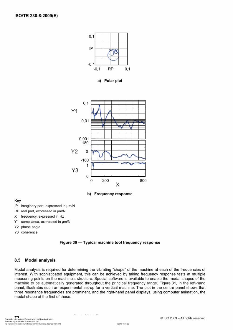
ISO/TR 230-8:2009(E)


RP 0,1

0,1

- 0,1 - 0,1

IP

a) Polar plot

0,1

0,01

0,001

0 200 800

180

- 180 0

1 0

X

Y1

Y2

Y3

b) Frequency response Key IP imaginary part, expressed in µm/N RP real part, expressed in µm/N X frequency, expressed in Hz Y1 compliance, expressed in µm/N Y2 phase angle Y3 coherence

Figure 30 — Typical machine tool frequency response

8.5 Modal analysis

Modal analysis is required for determining the vibrating “shape” of the machine at each of the frequencies of interest. With sophisticated equipment, this can be achieved by taking frequency response tests at multiple measuring points on the machine’s structure. Special software is available to enable the modal shapes of the machine to be automatically generated throughout the principal frequency range. Figure 31, in the left-hand panel, illustrates such an experimental set-up for a vertical machine. The plot in the centre panel shows that three resonance frequencies are prominent, and the right-hand panel displays, using computer animation, the modal shape at the first of these.



--`,,```,,,,````-`-`,,`,,`,`,,`---

ISO/TR 230-8:2009(E)


Without this type of equipment it is still possible to make a reasonable estimate of the principal modal shapes, albeit much more slowly. This can be achieved by using single-frequency sinusoidal excitation between tool holder and workpiece at each of the individual frequencies of interest. For the purpose of modal analysis, it is unimportant whether measurements are made of displacement, velocity or acceleration, providing that consistency is maintained. Simultaneous measurements are made at a reference point (close to the point of excitation) and at individual points over the entire structure. At each measurement point, the relative vibration value and phase difference with respect to the reference point should be determined. In addition, the location and orientation of each measurement point within the structure should be established and recorded. In this case, derivation of the mode shapes has to be made manually by inspection of the results28). It is, however, beyond the scope of this document to give further instruction in this procedure.

The direction of excitation is not critical, providing that the required modes can be excited. For example, modes occurring in the X direction and modes occurring in the Y direction may both be excited for the purpose of modal analysis by diagonal excitation (i.e. at 45°)29) midway between the two or even three directions, though this can sometimes introduce certain cross-response phase anomalies (see 8.6).

For each mode analysed, the following information should be provided:

⎯ frequency, in Hz;

⎯ direction of excitation;

⎯ description of mode;



⎯ axial positions of machine slides;

⎯ static preload;

⎯ machine mounting conditions.

The verbal description of the mode may be supplemented either with diagrams showing the maximum excursion of the various structural members or (preferably) with video clips of computer-generated animated displays. Video clips are particularly helpful in understanding complicated phase relationships.

8.6 Cross-response tests

For a more detailed (and more advanced) investigation into the structural behaviour of a machine, a complete examination of the vibration response in each direction, for each direction of excitation can yield valuable information. Figure 32 shows a “compliance matrix” for a vertical machine tool with the nine possible response vector diagrams. The number (and size) of lobes in each response equates to the number (and magnitude) of principal natural frequencies. Each response, or transfer function, G, is identified by suffixes indicating the directions of excitations and displacements. The main diagonal, Gxx, Gyy, Gzz, shows the polar plots for “direct response” in each direction.

The other plots are for “cross-responses”, where the displacement measurements are perpendicular to the excitation. It will be seen that all the cross-response plots go above the real axis (phase angle greater than 180°), and the point of crossing of the axis becomes significant in the estimation of structural stability to chatter, particularly with respect to coupled modes. (See 4.6.4.)

From these nine compliance frequency responses, the mode shapes for each resonance frequency with directions and magnitudes can be derived.

28) With acquired skill, a tester will be able to determine modal shapes using a pair of vibration transducers directly connected to a two-channel oscilloscope.

29) So long, of course, that an important mode at right angles (i.e. 45° the other way) does not exist!



--`,,```,,,,````-`-`,,`,,`,`,,`---

ISO/TR 230-8:2009(E)


Approximation of the geometry

of the machine tool structure

Evaluation of measured data (curve-fitting) Animation of the results

3

1 2

6

5 4F

YX

Z

° Measuring point (typical number of measuring points for machine tool structures: 200)

Determination of the modal parameters for the undamped natural frequencies ν1, ν2 …

Mode shapes at frequencies ν1, ν2 …

Analysis and elimination of dynamic weak points

Key 1 motor 2 column 3 headstock 4 slide 5 table 6 bed ° measuring point F excitation force

Figure 31 — Experimental procedure for modal analysis

8.7 “Non-standard” vibration modes

In the previous subclauses, the presentation of “standard” frequency and modal analyses has been confined to relative excitation between tool and workpiece. But in some cases, these may not be sufficient.

There can exist machine modes involving little or no relative movement between tool and workpiece, which cannot, therefore, be directly excited by either the cutting process or an exciter placed between the tool and workpiece. Depending on where their sources are located, these modes may still sometimes be excited by the operation of the machine. Gear and belt drives and other ancillary devices can excite structural vibrations away from the machining area and yet still produce palpable vibration and noise, if not surface finish problems.

If these types of problem are suspected, it is recommended that “absolute excitation” as described in 6.4 be used. This has the capability of exciting low-frequency “rocking” modes of machines on their foundations. It was also noted in 5.2 that modes excited by slide acceleration effects may have only a minimal response at the cutter location but could still be troublesome through their persistence. Again, such modes can be examined using absolute excitation.



--`,,```,,,,````-`-`,,`,,`,`,,`---

ISO/TR 230-8:2009(E)


Gzx

0,05 µm/NRe

Im0,05 µm/N

Gxx

0,05 µm/N

Re

Im0,05 µm/N Gxy

0,05 µm/N

Re

Im0,05 µm/N Gxz

0,05 µm/N

Re

Im0,05 µm/N

Gyx

0,05 µm/N

Re

Im0,05 µm/N Gyz

0,05 µm/N

Re

Im0,05 µm/N

Gzy

0,05 µm/N

Re

Im0,05 µm/N Gzz

0,05 µm/N

Re

Im0,05 µm/N

Gyy

0,05 µm/N

Re

Im0,05 µm/N

x

z

y

xxx xy xz

yx yy yz y

zx zy zz z

xyz

FG G GG G G FG G G F

⎧ ⎫⎧ ⎫ ⎡ ⎤⎪ ⎪ ⎪ ⎪⎢ ⎥= ⋅⎨ ⎬ ⎨ ⎬⎢ ⎥⎪ ⎪ ⎪ ⎪⎢ ⎥⎩ ⎭ ⎣ ⎦ ⎩ ⎭

Key Im imaginary part Re real part x, y, z displacement in respective coordinate direction Gi, j frequency response function with i = x, y, z, j = x, y, z i direction of excitation j direction of measured response Fx,y,z force in x, y, z

Figure 32 — Compliance matrix for a vertical milling machine

8.8 Providing standard stability tests

The provision of acceptable standard stability tests has yet to be achieved, and although it is fraught with difficulty, two approaches to this show possibilities. A series of acceptable cutting tests can be carried out by agreement between vendor and customer, as described in 7.4. This is probably the best pragmatic solution, but in no way can this constitute a standard procedure.

Alternatively, an “ideal” standard procedure can be envisaged comprising the measurement of the nine transfer functions of the machine (as shown in Figure 32), yielding three direct compliances and six cross-compliances. These could then be combined with the appropriate direction coefficient for different orientations of the cutting force, using specially developed computer programs.



--`,,```,,,,````-`-`,,`,,`,`,,`---

ISO/TR 230-8:2009(E)


Annex A (informative)

Overview and structure of this part of ISO 230

This annex explains how to use this part of ISO 230 by giving an overview of its structure and content.

Clause 4 presents fundamental concepts in the theory of vibrations and discusses the action of vibrating sources first on simple mechanical models, and later on machine tools themselves. In this clause, the emphasis is on understanding the types of response that can be generated in vibrating structures. A brief résumé of the contents of this clause is to be found in Annex C.

Clause 5 discusses the main types of vibration source likely to be encountered in machine tools. Where appropriate, the theory behind the mechanisms driving these sources is also discussed. Where the vibration sources generally lie outside the scope of the report, only a brief discussion is presented.

Clause 6 discusses instrumentation and general requirements for carrying out practical tests to evaluate machine tool vibrations.

Clause 7 presents a number of straightforward tests for evaluating the behaviour of the machine tool, subjected to the various types of vibration lying within the scope.

Clause 8 is concerned with special tests designed to study the machine tool structure through artificial excitation.

An alternative overview of the report is provided in Table A.1, which has been prepared for ease of reference. This gives clause/subclause references relating to the different types of vibration under specific subject headings.

A Technical Report of this nature necessarily introduces many terms with specialized meanings which are given in Clause 3.

Table A.1 — Cross-references for various sources of vibration

Vibration source Theoretical concepts Source description Practical testing Annex E examples

Unbalance 4.5.2, 4.5.4, 4.7.3, Annex B

5.1, 5.5.4 6.3.1, 6.4, 6.8, 7.1, 7.3.4, Annex D

4, 5

Acceleration of slides 4.5.4, 4.5.5, 4.7.2 5.2, 5.5.4 6.8, 7.2, 7.3.4, 8.7 6

External 4.1.3, 4.3.3 5.3 6.7, 6.8, 7.3 2, 3

Machining 4.4.3, 4.4.4, 4.6.2 5.4 6.8, 7.4 1

Artificial 4 — 8 —

Other sources 5.5 5.5 8.7 —



--`,,```,,,,````-`-`,,`,,`,`,,`---

ISO/TR 230-8:2009(E)


Annex B (informative)

Relationships between vibration parameters

Vibration may be measured as a displacement, velocity or acceleration depending on the type of transducer used. The Equations (1), (2) and (3) show the relationships between these quantities, which depend on frequency. Each of these quantities is represented by a sine wave as shown in Figure 1. (See also 6.5.)

From these equations, it is seen that the conversion between measuring units involves the processes of integration and differentiation thus:

displacement → {differentiated} → velocity → {differentiated} → acceleration

acceleration → {integrated} → velocity → {integrated} → displacement

Modern signal processing equipment usually has facilities for carrying out these procedures automatically. To achieve this by manual means, which is still sometimes required, use can be made of the nomogram shown in Figure B.1.

It should be understood from the outset, however, that the procedure involved is strictly valid for “pure” sine waves. To handle complex signals with significant harmonic distortion, it is necessary to process each harmonic separately. In practice, individual test measurements of displacement, velocity and acceleration often show considerable divergence from the relationships present here, because of the difficulty in ensuring that pure sine waves are achieved.

Figure B.1 is a nomogram showing the relationship between the four quantities: displacement, velocity, acceleration and frequency. When any two of these are known, the other two can be derived from the chart. Frequency (in Hz) is shown along the abscissa and velocity (in m/s) along the ordinate. Displacements (in metres) are shown along diagonal axes sloping up from left to right and accelerations in (m/s2) along diagonal axes sloping down from left to right.

Four examples should suffice to show how any two known quantities are used to derive the other two quantities:

⎯ Find the velocity and acceleration corresponding to a frequency of 5 Hz and a displacement of 0,003 m.

From 5 Hz on the bottom axis, draw a vertical line to meet the upward sloping diagonal for 0,003 m. The point of intersection corresponds to a velocity 0,094 m/s on the vertical axis and to an acceleration of approximately 3 m/s2 on the downward sloping diagonal.

⎯ Find the displacement and velocity corresponding to a frequency of 40 Hz and an acceleration of 200 m/s2.

From 40 Hz on the bottom axis, draw a vertical line to meet the downward sloping line for 200 m/s2. The point of intersection corresponds to a velocity of approximately 0,8 m/s on the vertical axis and to a displacement of 0,003 m on the upward sloping diagonal.

⎯ Find the displacement and acceleration corresponding to a frequency of 50 Hz and a velocity of 0,002 m/s.

From 50 Hz on the bottom axis, draw a vertical line to meet the horizontal line for 0,002 m. The point of intersection of the two diagonal lines gives 0,000 006 4 m (or 6,4 µm) displacement and 0,63 m/s2.

⎯ Find the frequency and acceleration corresponding to a displacement of 0,000 001 m and a velocity of 0,000 3 m/s.

From 0,000 3 m on the vertical axis, draw a horizontal line to meet the upward sloping line for 0,000 001 m. The point of intersection corresponds to 0,09 m/s2 on the downward diagonal and a frequency on the horizontal axis of approximately 48 Hz.



--`,,```,,,,````-`-`,,`,,`,`,,`---

ISO/TR 230-8:2009(E)


Key X frequency, Hz Y velocity, m/s

Velocity, displacement and acceleration, rms values (or peak values).

Figure B.1 — Nomogram showing relationship of vibration quantities for simple harmonic motion



--`,,```,,,,````-`-`,,`,,`,`,,`---

ISO/TR 230-8:2009(E)


Annex C (informative)

Summary of basic vibration theory

C.1 Theoretical background

This annex presents as a reference a short summary of the basic vibration theory presented in Clause 4.

C.2 Single-degree-of-freedom-systems

Machine tools are subject to both static and dynamic forces that can lead to deformations adversely affecting their performance. The dynamic compliance of a machine tool can be regarded as a major criterion in a machine’s response to dynamic forces.

Machine tools comprise several physical components, the machine bed, spindle heads, guide ways, etc., and should therefore be considered multi-degree-of-freedom systems from the vibration point of view. However, in most cases, the machine behaviour under dynamic load can be represented as a system of independent (modal) single-degree-of-freedom systems. The use of these very simple models enables a basic understanding of machine tool vibration to be achieved.

Figure C.1 shows an abstraction of this system and its mathematical description (equations of motion with the assumption of viscous damping).

G( jω) is the dynamic compliance (or transfer function) of the system and represents the complex quotient of displacement, x, and the respective dynamic force, F.

Further transformation leads to the non-complex formulae for the amplitude and the phase angle as shown in Technical Box 4.

In the case of a single-degree-of-freedom system, the dynamic compliance is completely defined by the three system parameters: static stiffness, k, undamped natural frequency, ω0, and the damping ratio, ζ.

A common graphical representation is the frequency response function in terms of displacement amplitude and phase angle shown on the left-hand side of Figure C.2. The excitation frequency determines not only the amplitude but also the time shift between the acting force and the respective displacement (phase angle).

Equivalent information can be obtained by means of a polar plot shown on the right-hand side of Figure C.2. The distance between the centre of the coordinate system and a point of the locus curve denotes the amplitude while the polar angle of this vector indicates the phase angle.

An illustrative explanation of the phenomena in terms of force equilibrium is depicted in Figure 8 in Clause 4.



--`,,```,,,,````-`-`,,`,,`,`,,`---

ISO/TR 230-8:2009(E)


m mass k stiffness c damping

Fstat static force Fdyn dynamic force x displacement x velocity x acceleration

Time domain

stat dyn stat dyn( )mx cx k x x F F+ + ⋅ + = + mx inertia force cx damping force

dynkx dynamic spring force

statkx static spring force

Transformation ˆ( ) j tF t F e ω⇒ ⋅ ( )ˆ( ) j tx t x j e ω ϕω +⇒ ⋅ ⋅

( )ˆ( ) j tx t x e ω ϕ+⇒ ⋅ 2 ( )ˆ( ) j tx t x j e ω ϕω +⇒ ⋅ ⋅

Frequency domain

2 ( ) ˆˆ ˆ ˆ( ) ( ) j t j tmx j cx j kx e Feω ϕ ωω ω +⎡ ⎤+ + ⋅ =⎣ ⎦

with 2 fω π= ⋅ ⋅

i ( )2

ˆ( ) ( ) 1( ) ˆ ( )( ) ( ) ( )x x jG j e

F jF m j c j kϕ ωω ωω

ωω ω ω= ⋅ = =

+ +

with 2n

km

ω = and n2

cm

ζω

=⋅ ⋅

222 2n n

1 1

( )( ) ( )( ) ( ) 1 2 1

k kG j m c j jj jk k

ωω ωω ω ζω ω

= =+ + + +

Conjugate complex extended

with n

ωηω

=

( )( ) ( ) ( ) ( )

2

2 22 22 2

1 21( )

1 2 1 2

k kG j j

ζη ηω

η ζη η ζη

⋅ − ⋅= −

− + − +

Figure C.1 — Model of a single-degree-of-freedom system (displacement response)



--`,,```,,,,````-`-`,,`,,`,`,,`---

ISO/TR 230-8:2009(E)


dynamic force ( )F jω

dynamic displacement ( )x jω

static compliance 1k

damping ratio n2

cm

ζω

=

max. dynamic compliance of the undamped system max

ˆ 1 1ˆ 2x

kF ζ⎧ ⎫ = ⋅⎨ ⎬⎩ ⎭

a) Frequency response b) Polar curve maxn

1 1 1ˆ ˆˆ mx F Fc k c ω

≈ ⋅ = ⋅ ⋅

Y1 compliance Y2 phase angle f frequency

ϕ phase angle Im imaginary part Re real part

k stiffness c damping m mass

ωn natural circular frequency

Figure C.2 — Displacement frequency response and polar plots for a single-degree system

Theoretically, three typical frequencies are to be distinguished as shown below:

⎯ natural frequency of the undamped system: nkm

ω =

(At this frequency, the phase shift between force and displacement is 90° and the acting force would be balanced only by the damping force as shown in Figure C.2. Without any damping, the amplitude of the system theoretically becomes infinite.)

⎯ natural frequency of the damped system: 2d n 1ω ω ζ= ⋅ −

⎯ resonance frequency of the damped system: 2r n 1 2ω ω ζ= ⋅ −

At this frequency, a real system subject to harmonic excitation has its maximum dynamic compliance (displacement amplitude).

For real machine tools, a quantitative distinction is usually not necessary since, due to a small damping ratio (ζ u 0,1), these three frequencies are more or less the same. The influence of different damping ratios is exemplified in Figure C.3.



--`,,```,,,,````-`-`,,`,,`,`,,`---

ISO/TR 230-8:2009(E)


Key Y1 dynamic magnification Y2 phase angle, expressed in degrees f frequency, expressed in Hz fn natural frequency D damping ratio (ζ )

Figure C.3 — Damping influence on a single-degree system displacement response

C.3 Complex systems

A machine tool is a complex dynamic system but its dynamic behaviour can easily be described mathematically when a linear system characteristic is assumed. For machine tools, this assumption is true in most cases. It means that the main parameters (masses, stiffnesses, damping ratios) do not change with time or with the motion itself.

In this case, the frequency response function of an overall system with several natural frequencies, i.e. resonance peaks, can be derived by means of the superposition of the frequency response functions of the individual modal single-degree-of-freedom systems. The frequency response function of the complex system is thus effectively the sum of the frequency response functions of the equivalent single-degree-of-freedom systems, each representing a specific natural frequency of the response. See Equation (25).

This procedure forms the basis for both the experimental and analytical modal analyses of vibrating structures.



--`,,```,,,,````-`-`,,`,,`,`,,`---

ISO/TR 230-8:2009(E)


Annex D (informative)

Spindle and motor balancing protocol

Correct balancing of rotating components is an essential requirement for minimizing machine-borne vibrations.

The same principles apply to motor and pulley balancing as to spindle and tooling balancing. In both cases, individual components should be balanced separately to ensure good interchangeability of parts. Assemblies that occasionally need to be dismantled should be balanced disassembled.

NOTE It is recognized that, for high-speed applications, this procedure can still result in an unacceptable balance condition, owing to the build-up of residual errors from the separate components. In this case, a final assembly balance should also be carried out.

For spindles and tooling:

⎯ Spindles should always be balanced with the drive keys fitted, but without tooling.

⎯ Tooling should always be separately balanced.

⎯ Milling cutters should be balanced to at least grade G40 in accordance with ISO 15641.

⎯ Grinding wheels should be balanced in accordance with ISO 6103.

For motors and pulleys:

For drives employing loose keys, the correct procedure is a little more complex.

⎯ The motor manufacturer is required to balance motors with a pre-balanced sleeve retaining a half-key in the keyway.

⎯ The pulley (or machine tool) manufacturer is required to furnish a test mandrel balanced with the same half-key that the motor manufacturer uses for the motor. This is most important.

⎯ Individual pulleys can then be balanced on the mandrel with the full key supplied, which need bear no relation to the half-key used for balancing the motor and mandrel.

⎯ The pulley is now fitted to the motor with the supplied full key.

By this means, replacement pulleys and keys can easily be balanced.



--`,,```,,,,````-`-`,,`,,`,`,,`---

ISO/TR 230-8:2009(E)


Annex E (informative)

Examples of test results and their presentation

This annex provides illustrations showing how some of the vibration test work can be carried out. It should be clearly understood that these are examples only, and that the user of this document is under no obligation to reproduce the methods shown.

EXAMPLE 1 Measuring absolute vibration on a cylindrical grinding machine (during machining) to obtain relative vibration displacement amplitudes between wheel and workpiece.

If the measurement of relative vibration between tool and workpiece is difficult to achieve, simultaneous (absolute) vibration measurements at several points may be used. This example shows a calculation method for obtaining the relative vibration vector in the X direction between wheel head and workpiece on a cylindrical grinding machine.

NOTE The dynamic properties of the workpiece may affect the relative vibration characteristics of the machining process.

Vibration vectors30) are measured with transducers at dx1 on the wheel head, dx2 on the headstock and dx3 on the footstock in the same direction, X. The lateral separations of vibration transducers in the Z direction are a and b as shown in Figure E.1.

The relative vibration vector is taken as the difference between the absolute levels of the vibration vectors at the wheel head and workpiece. The workpiece vibration vector is obtained by linear interpolation from the vectors at the headstock and footstock ends, as shown in Technical Box 11.

The amplitudes, d, and phase angles, α, are measured simultaneously at the three points and are used to replace the vectors in Technical Box 11. Phase angles are measured relative to the wheel head reference point, which means that α1 is zero and can therefore be omitted. Note that, in this application, all the displacement amplitudes and phase angles must be measured simultaneously in order to obtain a correct value for the relative vibration.

30) Vectors require two components to be measured; in this case, amplitude and phase angle are used.



--`,,```,,,,````-`-`,,`,,`,`,,`---

ISO/TR 230-8:2009(E)


Key 1 wheel-head 2 wheel 3 workpiece 4 headstock 5 footstock 6 bed 7 vibration tranducers (dx1, dx2, dx3)

Figure E.1 — Testing vibration on cylindrical grinding machine



--`,,```,,,,````-`-`,,`,,`,`,,`---

ISO/TR 230-8:2009(E)


x2 x3x x1

+= −

+bd ad

d da b

This gives the following relationship:

x2 2 x3 3x x1

2 2x

x2 2 x3 3x1

x2 2 x3 3

cos( ) cos( )sin( ) cos( )

, wherecos cos

sin sin

bd t ad td t d t

a b

d p qbd ad

p da b

bd adq

a b

ω α ω αω φ ω

α α

α α

− + −+ = −

+

∴ = +

+= −

++

= −+

where

dx is the relative vibration amplitude;

α is the phase angle;

ω = 2πN/60, where N is wheel rotation speed in rpm;

ϕ is the resulting phase angle of relative vibration;

t is the time in seconds.

Technical Box 11 — Deriving relative vibrations



--`,,```,,,,````-`-`,,`,,`,`,,`---

ISO/TR 230-8:2009(E)


EXAMPLE 2 Measuring vibration occurring externally to the machine in the time domain.

a) X direction

b) Y direction

Figure E.2 (continued)



--`,,```,,,,````-`-`,,`,,`,`,,`---

ISO/TR 230-8:2009(E)


c) Z direction

Key t time, expressed in s d displacement, expressed in µm

Figure E.2 — Environmental vibration test results (200 Hz sample rate)

Maximum peak-to-peak vibration value: 0,1 µm.

Direction of maximum vibration: X.

Duration of test: 5 s.

Test equipment: three-channel displacement measuring system using capacitance gauges measuring against the cylindrical target mounted on the spindle.

Machine: five-axis vertical spindle machining centre. Three linear slides are stacked on the bed to carry the spindle. The workpiece is mounted on the compound rotary table attached to bed.

Location and date of test: Machine shop, 2003-11-XX.

Environmental conditions of test: Typical machine shop environment — quiet.

External operations: Typical machine shop environment, no heavy equipment operating close to the machine.

Status of the machine under test: Powered down, auxiliary equipment off.



--`,,```,,,,````-`-`,,`,,`,`,,`---

ISO/TR 230-8:2009(E)


EXAMPLE 3 Measuring vibration occurring externally to the machine in the frequency domain.

Key A vibrations from a hydraulic unit dy displacement amplitude (dimensionless units) f frequency, expressed in Hz vS spindle speed, expressed in r/min

Figure E.3 — Machine spindle spectra influenced by external hydraulic unit

Figure E.3 shows the resultant frequency spectra of a machine tool over a range of spindle speeds. The speed-independent peaks with approximately 270 Hz can be attributed to vibrations of an external hydraulic unit.



--`,,```,,,,````-`-`,,`,,`,`,,`---

ISO/TR 230-8:2009(E)


EXAMPLE 4 Out-of-balance vibration measured at the spindle snout using the grade test method described in Clause 7.

Key v peak vibration velocity, expressed in Hz vS spindle speed, expressed in r/min

Figure E.4 — Out-of-balance vibration at spindle nose, showing peak vibration velocity against spindle speed for three pulley ratios

This example shows the vibration velocity over a range of spindle speeds, measured on a machining centre fitted with three discrete pulley ratios between motor and spindle. This machine had a natural resonance of the spindle carrier at 175 Hz.

a) 2:1 reduction for the “high torque” version. The motor speed was thus twice that of the spindle and the peak vibration at 75 Hz (4 500 r/min) was caused by motor out-of-balance at 9 000 r/min. The grade value was G2,5.

b) 1:1 pulley ratio for the “standard” version. The grade value was 4.

c) 4:5 step-up ratio for the “high speed” version. This was beginning to excite the first carrier resonance at 175 Hz as top speed was approached. The grade value was 4.



--`,,```,,,,````-`-`,,`,,`,`,,`---

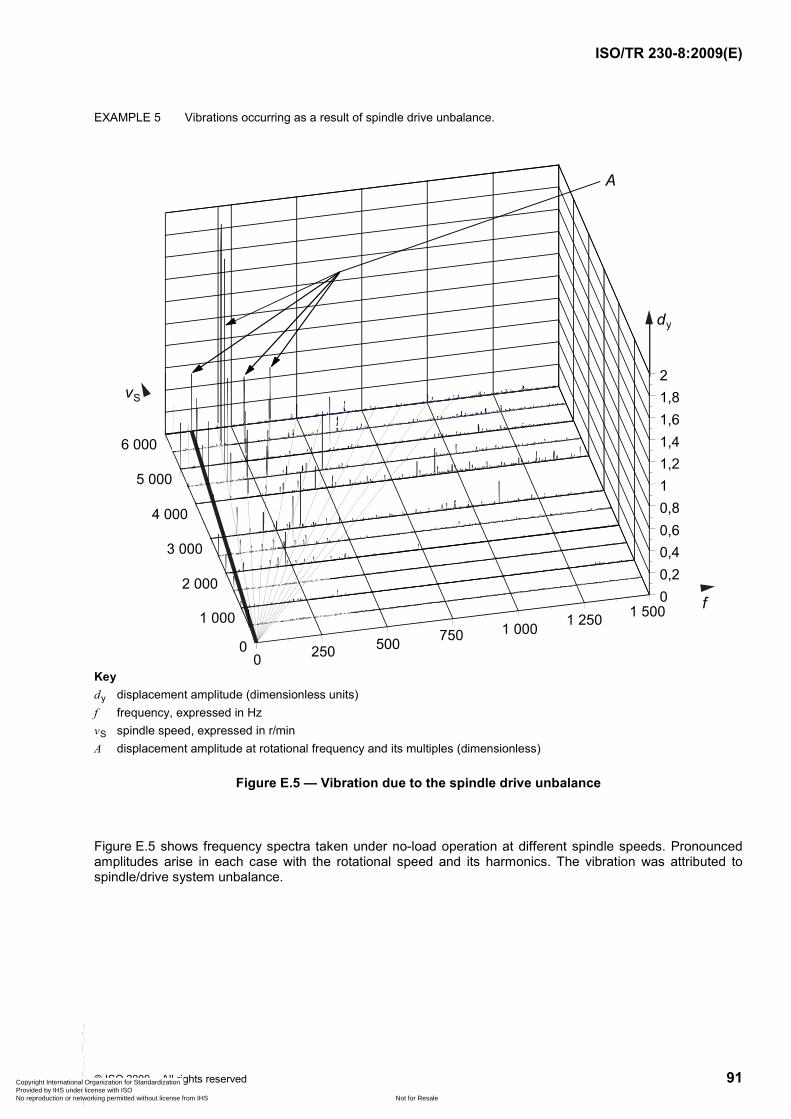
ISO/TR 230-8:2009(E)


EXAMPLE 5 Vibrations occurring as a result of spindle drive unbalance.

0 250 500 750 1 000 1 250 1 500

0

1 000

2 000

3 000

4 000

5 000

6 000

00,20,40,60,811,21,41,61,82

vS

d

A

f

y

Key dy displacement amplitude (dimensionless units) f frequency, expressed in Hz vS spindle speed, expressed in r/min A displacement amplitude at rotational frequency and its multiples (dimensionless)

Figure E.5 — Vibration due to the spindle drive unbalance

Figure E.5 shows frequency spectra taken under no-load operation at different spindle speeds. Pronounced amplitudes arise in each case with the rotational speed and its harmonics. The vibration was attributed to spindle/drive system unbalance.



--`,,```,,,,````-`-`,,`,,`,`,,`---

ISO/TR 230-8:2009(E)


EXAMPLE 6 Vibration caused by a moving machine slide.

Vertical machining centre: XXXXX

CNC: XXXXX

Vertical straightness of Y (EZY), Y feed: 0/200 mm/min (solid line) and 0/5 000 mm/min (dotted line)

Acceleration: 0,25 m/s2 (solid line) and 2,2 m/s2 (dotted line)

Y (mm)

EZY

(µm

)

Figure E.6 — Vibration caused by accelerating a machine slide

The example in Figure E.6 shows the results obtained with a two-dimensional scale on a 100 mm movement of a linear axis (“Y”) at feed rates and accelerations of 0 mm/min to 200 mm/min and 0,25 m/s2 (solid line), and 0 mm/min to 5 000 mm/min (dotted line) and 2,2 mm/s2 (dotted line).

Interpretation

Owing to the acceleration at the start and stop points, peaks appear in the measured straightness of the movement along the Y axis.

For the higher feed rate, the (higher) acceleration continues for longer and results in a much higher vibration displacement amplitude.



--`,,```,,,,````-`-`,,`,,`,`,,`---

ISO/TR 230-8:2009(E)


Bibliography

[1] ISO 10814:1996, Mechanical vibration — Susceptibility and sensitivity of machines to unbalance

[2] ISO 10816-1:1995, Mechanical vibration — Evaluation of machine vibration by measurements on non-rotating parts — Part 1: General guidelines

[3] ISO 10816-3:1998, Mechanical vibration — Evaluation of machine vibration by measurements on non-rotating parts — Part 3: Industrial machines with nominal power above 15 kW and nominal speeds between 120 r/min when measured in situ

[4] ISO 13373-2:2005, Condition monitoring and diagnostics of machines — Vibration condition monitoring — Part 2: Processing, analysis and presentation of vibration data

[5] WECK, M., 2001, Werkzeugmaschinen Fertigungssysteme 5, Messetechnische Untersuching und Beurteilung, springer, Berlin, Heidelberg, New York

[6] HOLZWEIßIG, F., DRESIG, H., 1994, Lehrbuch der Maschinenendynamik, Fachbuchverlag, Leipzig, Köln

[7] EWINS, D.J.; 1986, Modal Testing: Theory and Practice, Research Studies Ltd., Letchworth, England, 1986

[8] NATKE, H.G., 1992, Einführung in die Theorie und Praxis der Zeitreihen- und Modalanalyse; Wiesbaden, Vieweg Verlag

[9] DEN HARTOG, J.P., 1985, Mechanical Vibrations, Dover Publications, Mineola, N.Y. (Original edition: 1934, McGraw-Hill Book Company, New York)

[10] TOBIAS, S.A., 1961, Machine-Tool Vibration, Blackie & Son Ltd., Glasgow, 1965. (Originally published in German as “Schwingungen an Werkzeugmaschinen” by Carl Hanser Verlag, Munich, 1961.) Currently out of print

[11] PETERS, J., 1965, “Damping in Machine Tool Construction”, 6th MTDR Conference, 1965, pp 23-26

[12] TLUSTY and POLACEK, 1963, “The Stability of Machine Tools against Self-excited Vibration in Machining”, Proceedings of the International Research in Production Engineering, Pittsburgh, 1963

[13] TLUSTY, G., 1999, Manufacturing Processes and Equipment, Prentice Hall, 1st edition, 1999



--`,,```,,,,````-`-`,,`,,`,`,,`---

ISO/TR 230-8:2009(E)

ICS 25.080.01 Price based on 93 pages

© ISO 2009 – All rights reserved



--`,,```,,,,````-`-`,,`,,`,`,,`---

Documents

TECHNICAL ISO/TR REPORT 230-8allaboutmetallurgy.com/wp/wp-content/uploads/2016/12/… · · 2017-01-301) In some cases, practical considerations require that real or dummy tooling