Embed Size (px)
Citation preview

TechnicalInformation MX100 Performance Specifications
TI 04M08B01-00E
TI 04M08B01-00E©Copyright Mar. 20032nd Edition Sep. 2005
2
All Rights Reserved. Copyright © 2003, Yokogawa Electric Corporation
<Int> <Ind> <Rev>
TI 04M08B01-00E Sep. 30, 2005-00
CONTENTS
TI 04M08B01-00E 2nd Edition
MX100 Performance Specifications
Foreword .............................................................................................................. 3
1. Resolution of A/D Conversion ................................................................... 4
2. Accuracy of Reference Junction Compensation when MeasuringNegative Temperatures .............................................................................. 5
3. Withstand Voltages (Insulation) of MX System......................................... 6
4. Noise Rejection Performance of the MX System...................................... 8
5. Time Stamping of MX System ..................................................................17
6. Using Strain Conversion Cables (DV450-001) .........................................27
7. Computing Functions of Yokogawa-Developed PC Software .................317.1 Examples: Controlling Operation Using Properties of Measurement
Channels ................................................................................. 33
7.2 Examples: Counting Events .................................................................... 36
7.3 Examples: Using Time .............................................................................. 37
7.4 Examples: Calculating Statistics ............................................................. 38
7.5 Examples: Operation, Output (Release 2 or Later) ................................. 40
7.6 Examples: Miscellaneous ........................................................................ 42
7.7 Notes When Writing Computational Expressions and Techniques toAvoid Problems (Description) .................................................................. 43
8. Comparison between Functions of MX100 and DARWIN DA100 DataAcquisition Units ......................................................................................50
All Rights Reserved. Copyright © 2003, Yokogawa Electric Corporation TI 04M08B01-00E
3<Toc> <Ind> <Rev> Foreword
Sep. 30, 2005-00
ForewordThis technical information brochure addresses hard-to-understand and important items, amongthe general specifications of the MX100 PC-based data acquisition unit. When selecting theseitems, the editorial staff also referred to the content of FAQs it has received from users regardingthe DARWIN series systems. Yokogawa Electric hopes this brochure will be helpful for readers insolving problems that may be encountered when using the MX100.
The editorial staff plans to update this brochure as necessary, in keeping with the expansion offunctions provided the MX series of units, as well as according to user feedback. Your input ofcomments and requests to the Product Marketing Department of the Network Solutions BusinessDivision of Yokogawa Electric Corporation regarding this brochure will be greatly appreciated.
For inquiries, please contact us at:
E-mail: [email protected]
4
All Rights Reserved. Copyright © 2003, Yokogawa Electric Corporation
<Toc> <Ind>
TI 04M08B01-00E
1. Resolution of A/D Conversion
Sep. 30, 2005-00
1. Resolution of A/D ConversionThe A/D conversion resolution of the MX110-UNV-H04 high-speed universal input module andMX110-UNV-M10 medium-speed universal input module is specified as 16 bits (±20000/6000).This section briefly explains what this specification means.
Since 16 bits = 216 = 65536, you may consider that the measured value has a resolution of 1/65536 for the given measuring range. In the MX system, however, the measured value is shownat a resolution of ±20000, i.e., 1/40000, or at a resolution of ±6000, i.e., 1/12000, for a givenmeasuring range, in order to provide the highest resolution easily understandable to humans. Adetermination as to whether the input signal is measured at ±20000 or ±6000, is made dependingon which of them is better suited for the given measuring range. For example, the data sheetstates that the highest resolution is 100 µV (0.1 mV) (= 4 V/40000) for the 2 V range (-2 V to +2 V)and 1 mV (= 12 V/12000) for the 6 V range (-6 V to +6 V).
On the other hand, there are two particular ranges, among the measuring ranges of the MXsystem, at which the input signal is measured with a resolution of 1/60000. These are the 60 mV(0 to 60 mV) and 6 V (0 to 6 V) ranges indicated in the Special Input Range section of thespecifications sheet. By limiting the input ranges to the positive side only, their resolution is thusmade one order of magnitude higher than that of the standard 60 mV and 6 V ranges.Specifically, the highest resolution of the 6 V range is 100 µV (0.1 mV) (= 6 V/60000). Note thatthese special input ranges are only available with the optional software MXLOGGER, one of thegenuine Yokogawa line of software products.
All Rights Reserved. Copyright © 2003, Yokogawa Electric Corporation TI 04M08B01-00E
5<Toc> <Ind> 2. Accuracy of Reference Junction Compensation when Measuring Negative Temperatures
Sep. 30, 2005-00
2. Accuracy of Reference Junction Compensationwhen Measuring Negative TemperaturesThe Reference Junction Compensation Accuracy section of the specifications sheet indicatesaccuracy values, such as ±1°C and ±0.5°C, with the condition “when measuring 0°C or higher.”However, what values would the reference junction compensation accuracy have if negativetemperatures were measured?
The reference junction compensation accuracy deteriorates when negative temperatures aremeasured. (This statement is made based on the premise that the object of temperaturemeasurement is subject to a negative temperature, rather than that the main module of the MXsystem is subject to a negative temperature. Note that the operating temperature range of themain module is specified as 0 to 50°C.)
In the MX system, transistors are used as the reference junction compensators. The transistorgenerates a voltage according to the temperature of the measuring instrument’s terminals. Fromthis voltage and the voltage (thermoelectromotive force) provided by a thermocouple used foractual measurement, a voltage (thermoelectromotive force) when the reference junction is at 0°Cis calculated. This voltage is cross-checked with the thermoelectromotive force curve of thethermocouple being used, and output as a temperature value.
At this point, let us consider the question, “Why does the reference junction compensationaccuracy deteriorate on the negative temperature side?”
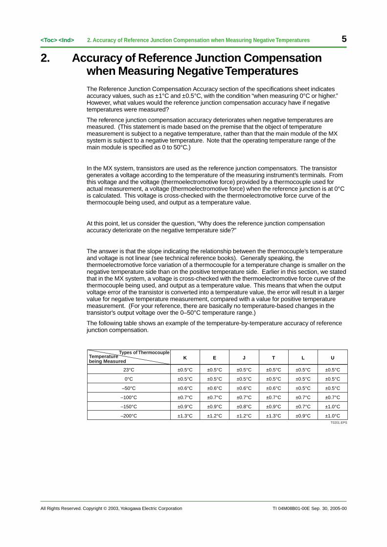
The answer is that the slope indicating the relationship between the thermocouple’s temperatureand voltage is not linear (see technical reference books). Generally speaking, thethermoelectromotive force variation of a thermocouple for a temperature change is smaller on thenegative temperature side than on the positive temperature side. Earlier in this section, we statedthat in the MX system, a voltage is cross-checked with the thermoelectromotive force curve of thethermocouple being used, and output as a temperature value. This means that when the outputvoltage error of the transistor is converted into a temperature value, the error will result in a largervalue for negative temperature measurement, compared with a value for positive temperaturemeasurement. (For your reference, there are basically no temperature-based changes in thetransistor’s output voltage over the 0–50°C temperature range.)
The following table shows an example of the temperature-by-temperature accuracy of referencejunction compensation.
23°C
0°C
–50°C
–100°C
–150°C
–200°C
±0.5°C
K
±0.5°C
±0.6°C
±0.7°C
±0.9°C
±1.3°C
±0.5°C
E
±0.5°C
±0.6°C
±0.7°C
±0.9°C
±1.2°C
±0.5°C
J
±0.5°C
±0.6°C
±0.7°C
±0.8°C
±1.2°C
±0.5°C
T
±0.5°C
±0.6°C
±0.7°C
±0.9°C
±1.3°C
±0.5°C
L
±0.5°C
±0.5°C
±0.7°C
±0.7°C
±0.9°C
±0.5°C
U
±0.5°C
±0.5°C
±0.7°C
±1.0°C
±1.0°CT0201.EPS
Types of ThermocoupleTemperature being Measured
6
All Rights Reserved. Copyright © 2003, Yokogawa Electric Corporation
<Toc> <Ind>
TI 04M08B01-00E
3. Withstand Voltages (Insulation) of MX System
Sep. 30, 2005-00
3. Withstand Voltages (Insulation) of MX System
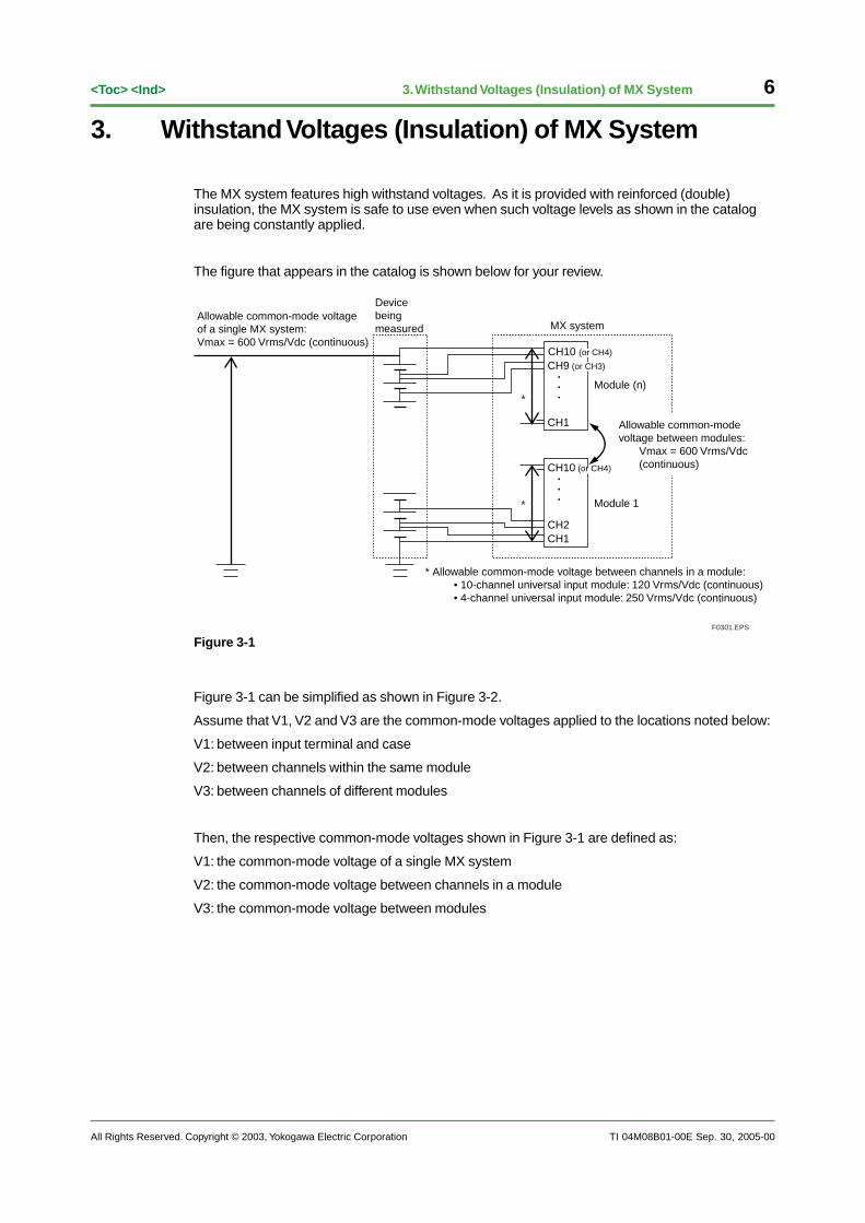
The MX system features high withstand voltages. As it is provided with reinforced (double)insulation, the MX system is safe to use even when such voltage levels as shown in the catalogare being constantly applied.
The figure that appears in the catalog is shown below for your review.
CH10 (or CH4)
CH9 (or CH3)•••
CH1
CH1CH2
CH10 (or CH4)•••
*
F0301.EPS
Allowable common-mode voltage of a single MX system:Vmax = 600 Vrms/Vdc (continuous)
Device being measured MX system
Module (n)
Allowable common-mode voltage between modules:
Vmax = 600 Vrms/Vdc (continuous)
Module 1
* Allowable common-mode voltage between channels in a module:• 10-channel universal input module: 120 Vrms/Vdc (continuous)• 4-channel universal input module: 250 Vrms/Vdc (continuous)
*
Figure 3-1
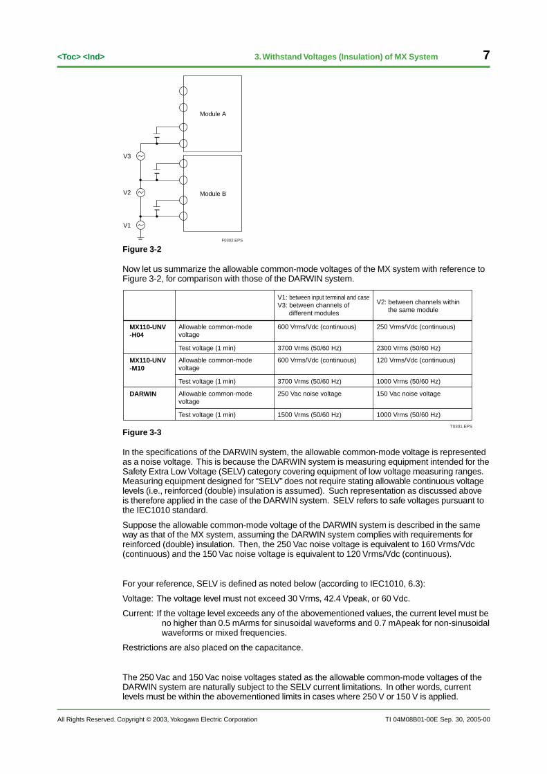
Figure 3-1 can be simplified as shown in Figure 3-2.
Assume that V1, V2 and V3 are the common-mode voltages applied to the locations noted below:
V1: between input terminal and case
V2: between channels within the same module
V3: between channels of different modules
Then, the respective common-mode voltages shown in Figure 3-1 are defined as:
V1: the common-mode voltage of a single MX system
V2: the common-mode voltage between channels in a module
V3: the common-mode voltage between modules
All Rights Reserved. Copyright © 2003, Yokogawa Electric Corporation TI 04M08B01-00E
7<Toc> <Ind> 3. Withstand Voltages (Insulation) of MX System
Sep. 30, 2005-00
Module B
Module A
V3
V2
V1
F0302.EPS
Figure 3-2
Now let us summarize the allowable common-mode voltages of the MX system with reference toFigure 3-2, for comparison with those of the DARWIN system.
Test voltage (1 min)
Allowable common-mode voltage
MX110-UNV-H04
MX110-UNV-M10
DARWIN
Allowable common-mode voltage
Test voltage (1 min)
Allowable common-mode voltage
Test voltage (1 min)
600 Vrms/Vdc (continuous)
V1: between input terminal and caseV3: between channels of
different modules
V2: between channels within the same module
3700 Vrms (50/60 Hz) 2300 Vrms (50/60 Hz)
600 Vrms/Vdc (continuous)
3700 Vrms (50/60 Hz)
250 Vac noise voltage
1500 Vrms (50/60 Hz)
250 Vrms/Vdc (continuous)
120 Vrms/Vdc (continuous)
1000 Vrms (50/60 Hz)
150 Vac noise voltage
1000 Vrms (50/60 Hz)
T0301.EPS
Figure 3-3
In the specifications of the DARWIN system, the allowable common-mode voltage is representedas a noise voltage. This is because the DARWIN system is measuring equipment intended for theSafety Extra Low Voltage (SELV) category covering equipment of low voltage measuring ranges.Measuring equipment designed for “SELV” does not require stating allowable continuous voltagelevels (i.e., reinforced (double) insulation is assumed). Such representation as discussed aboveis therefore applied in the case of the DARWIN system. SELV refers to safe voltages pursuant tothe IEC1010 standard.
Suppose the allowable common-mode voltage of the DARWIN system is described in the sameway as that of the MX system, assuming the DARWIN system complies with requirements forreinforced (double) insulation. Then, the 250 Vac noise voltage is equivalent to 160 Vrms/Vdc(continuous) and the 150 Vac noise voltage is equivalent to 120 Vrms/Vdc (continuous).
For your reference, SELV is defined as noted below (according to IEC1010, 6.3):
Voltage: The voltage level must not exceed 30 Vrms, 42.4 Vpeak, or 60 Vdc.
Current: If the voltage level exceeds any of the abovementioned values, the current level must beno higher than 0.5 mArms for sinusoidal waveforms and 0.7 mApeak for non-sinusoidalwaveforms or mixed frequencies.
Restrictions are also placed on the capacitance.
The 250 Vac and 150 Vac noise voltages stated as the allowable common-mode voltages of theDARWIN system are naturally subject to the SELV current limitations. In other words, currentlevels must be within the abovementioned limits in cases where 250 V or 150 V is applied.
8
All Rights Reserved. Copyright © 2003, Yokogawa Electric Corporation
<Toc> <Ind>
TI 04M08B01-00E
4. Noise Rejection Performance of the MX System
Sep. 30, 2005-00
4. Noise Rejection Performance of the MX SystemThe MX system includes a two-stage noise rejection function involving an A/D conversion method(integrating A/D) and a firmware-based first-order lag filter. The following is a description of thenoise rejection function implemented through the A/D conversion method focusing on the normalmode rejection ratio (NMRR) and common rejection ratio (CMRR) used as indices of the noiseresistance performance.
• Integrating A/D Converters and their Noise Rejection Performance
An integrating A/D converter integrates measured values over a specified length of time. It ispossible to remove a frequency component you wish to eliminate if the specified time lengthagrees with the period of that frequency component.
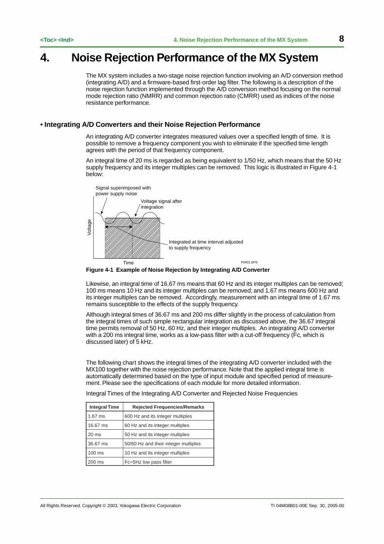
An integral time of 20 ms is regarded as being equivalent to 1/50 Hz, which means that the 50 Hzsupply frequency and its integer multiples can be removed. This logic is illustrated in Figure 4-1below:
Vol
tage
Time F0401.EPS
Signal superimposed with power supply noise
Voltage signal after integration
Integrated at time interval adjusted to supply frequency
Figure 4-1 Example of Noise Rejection by Integrating A/D Converter
Likewise, an integral time of 16.67 ms means that 60 Hz and its integer multiples can be removed;100 ms means 10 Hz and its integer multiples can be removed; and 1.67 ms means 600 Hz andits integer multiples can be removed. Accordingly, measurement with an integral time of 1.67 msremains susceptible to the effects of the supply frequency.
Although integral times of 36.67 ms and 200 ms differ slightly in the process of calculation fromthe integral times of such simple rectangular integration as discussed above, the 36.67 integraltime permits removal of 50 Hz, 60 Hz, and their integer multiples. An integrating A/D converterwith a 200 ms integral time, works as a low-pass filter with a cut-off frequency (Fc, which isdiscussed later) of 5 kHz.
The following chart shows the integral times of the integrating A/D converter included with theMX100 together with the noise rejection performance. Note that the applied integral time isautomatically determined based on the type of input module and specified period of measure-ment. Please see the specifications of each module for more detailed information.
Integral Times of the Integrating A/D Converter and Rejected Noise Frequencies
Integral Time
1.67 ms
16.67 ms
20 ms
36.67 ms
100 ms
200 ms
Rejected Frequencies/Remarks
600 Hz and its integer multiples
60 Hz and its integer multiples
50 Hz and its integer multiples
50/60 Hz and their integer multiples
10 Hz and its integer multiples
Fc=5Hz low pass filter
All Rights Reserved. Copyright © 2003, Yokogawa Electric Corporation TI 04M08B01-00E
9<Toc> <Ind> 4. Noise Rejection Performance of the MX System
Sep. 30, 2005-00
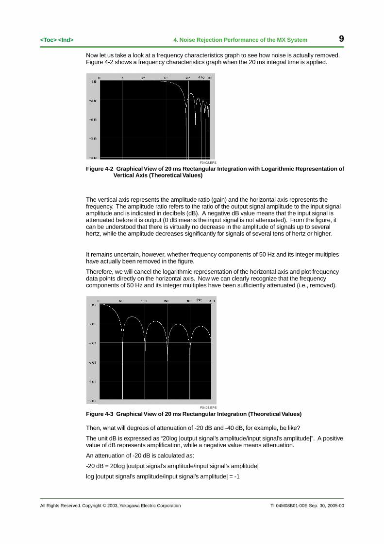
Now let us take a look at a frequency characteristics graph to see how noise is actually removed.Figure 4-2 shows a frequency characteristics graph when the 20 ms integral time is applied.
F0402.EPS
Figure 4-2 Graphical View of 20 ms Rectangular Integration with Logarithmic Representation ofVertical Axis (Theoretical Values)
The vertical axis represents the amplitude ratio (gain) and the horizontal axis represents thefrequency. The amplitude ratio refers to the ratio of the output signal amplitude to the input signalamplitude and is indicated in decibels (dB). A negative dB value means that the input signal isattenuated before it is output (0 dB means the input signal is not attenuated). From the figure, itcan be understood that there is virtually no decrease in the amplitude of signals up to severalhertz, while the amplitude decreases significantly for signals of several tens of hertz or higher.
It remains uncertain, however, whether frequency components of 50 Hz and its integer multipleshave actually been removed in the figure.
Therefore, we will cancel the logarithmic representation of the horizontal axis and plot frequencydata points directly on the horizontal axis. Now we can clearly recognize that the frequencycomponents of 50 Hz and its integer multiples have been sufficiently attenuated (i.e., removed).
F0403.EPS
Figure 4-3 Graphical View of 20 ms Rectangular Integration (Theoretical Values)
Then, what will degrees of attenuation of -20 dB and -40 dB, for example, be like?
The unit dB is expressed as “20log |output signal’s amplitude/input signal’s amplitude|”. A positivevalue of dB represents amplification, while a negative value means attenuation.
An attenuation of -20 dB is calculated as:
-20 dB = 20log |output signal’s amplitude/input signal’s amplitude|
log |output signal’s amplitude/input signal’s amplitude| = -1
10
All Rights Reserved. Copyright © 2003, Yokogawa Electric Corporation
<Toc> <Ind>
TI 04M08B01-00E
4. Noise Rejection Performance of the MX System
Output signal’s amplitude/input signal’s amplitude = 1/10
Likewise, -40 dB is calculated as an attenuation of 1/100, -6 dB as 1/2, and -3 dB as 1/��2.
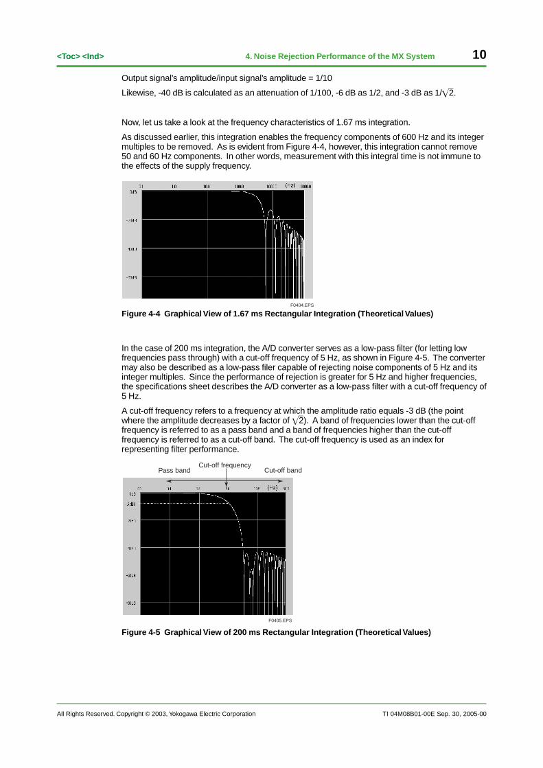
Now, let us take a look at the frequency characteristics of 1.67 ms integration.
As discussed earlier, this integration enables the frequency components of 600 Hz and its integermultiples to be removed. As is evident from Figure 4-4, however, this integration cannot remove50 and 60 Hz components. In other words, measurement with this integral time is not immune tothe effects of the supply frequency.
F0404.EPS
Figure 4-4 Graphical View of 1.67 ms Rectangular Integration (Theoretical Values)
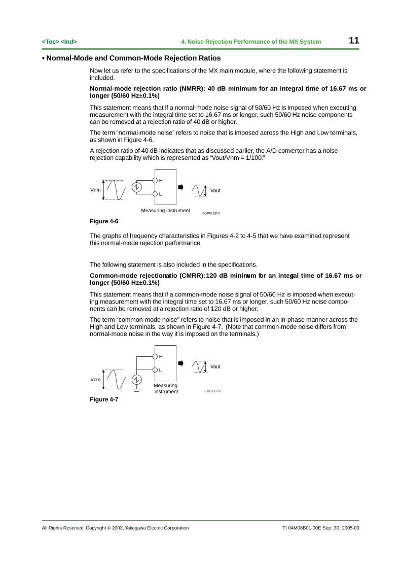
In the case of 200 ms integration, the A/D converter serves as a low-pass filter (for letting lowfrequencies pass through) with a cut-off frequency of 5 Hz, as shown in Figure 4-5. The convertermay also be described as a low-pass filer capable of rejecting noise components of 5 Hz and itsinteger multiples. Since the performance of rejection is greater for 5 Hz and higher frequencies,the specifications sheet describes the A/D converter as a low-pass filter with a cut-off frequency of5 Hz.
A cut-off frequency refers to a frequency at which the amplitude ratio equals -3 dB (the pointwhere the amplitude decreases by a factor of ��2). A band of frequencies lower than the cut-offfrequency is referred to as a pass band and a band of frequencies higher than the cut-offfrequency is referred to as a cut-off band. The cut-off frequency is used as an index forrepresenting filter performance.
F0405.EPS
Cut-off frequencyPass band Cut-off band
Figure 4-5 Graphical View of 200 ms Rectangular Integration (Theoretical Values)
Sep. 30, 2005-00
All Rights Reserved. Copyright © 2003, Yokogawa Electric Corporation TI 04M08B01-00E
11<Toc> <Ind> 4. Noise Rejection Performance of the MX System
• Normal-Mode and Common-Mode Rejection Ratios
Now let us refer to the specifications of the MX main module, where the following statement isincluded.
Normal-mode rejection ratio (NMRR): 40 dB minimum for an integral time of 16.67 ms orlonger (50/60 Hz ±0.1%)
This statement means that if a normal-mode noise signal of 50/60 Hz is imposed when executingmeasurement with the integral time set to 16.67 ms or longer, such 50/60 Hz noise componentscan be removed at a rejection ratio of 40 dB or higher.
The term “normal-mode noise” refers to noise that is imposed across the High and Low terminals,as shown in Figure 4-6.
A rejection ratio of 40 dB indicates that as discussed earlier, the A/D converter has a noiserejection capability which is represented as “Vout/Vnm = 1/100.”
VoutVnm
H
L
Measuring instrumentF0406.EPS
Figure 4-6
The graphs of frequency characteristics in Figures 4-2 to 4-5 that we have examined representthis normal-mode rejection performance.
The following statement is also included in the specifications.
Common-mode rejection ratio (CMRR): 120 dB minimum for an integral time of 16.67 ms orlonger (50/60 Hz ±0.1%)
This statement means that if a common-mode noise signal of 50/60 Hz is imposed when execut-ing measurement with the integral time set to 16.67 ms or longer, such 50/60 Hz noise compo-nents can be removed at a rejection ratio of 120 dB or higher.
The term “common-mode noise” refers to noise that is imposed in an in-phase manner across theHigh and Low terminals, as shown in Figure 4-7. (Note that common-mode noise differs fromnormal-mode noise in the way it is imposed on the terminals.)
Vout
Vcm
H
L
Measuring instrument F0407.EPS
Figure 4-7
Sep. 30, 2005-00
12
All Rights Reserved. Copyright © 2003, Yokogawa Electric Corporation
<Toc> <Ind>
TI 04M08B01-00E
4. Noise Rejection Performance of the MX System
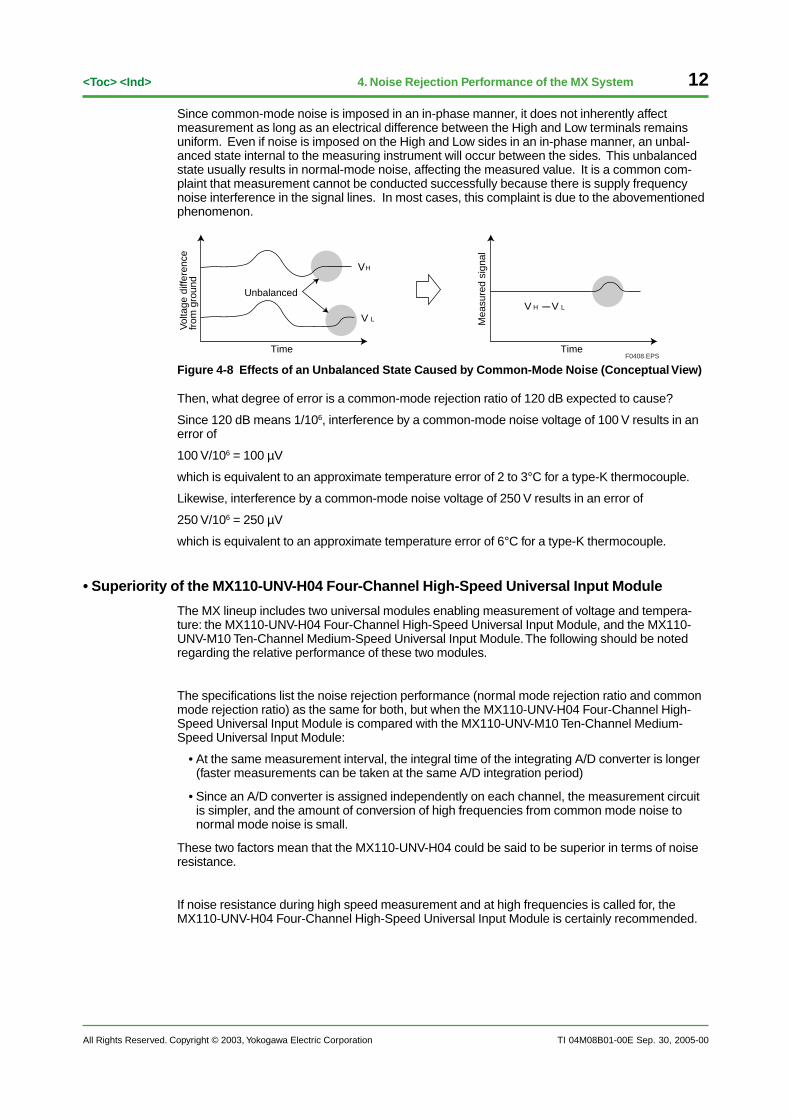
Since common-mode noise is imposed in an in-phase manner, it does not inherently affectmeasurement as long as an electrical difference between the High and Low terminals remainsuniform. Even if noise is imposed on the High and Low sides in an in-phase manner, an unbal-anced state internal to the measuring instrument will occur between the sides. This unbalancedstate usually results in normal-mode noise, affecting the measured value. It is a common com-plaint that measurement cannot be conducted successfully because there is supply frequencynoise interference in the signal lines. In most cases, this complaint is due to the abovementionedphenomenon.
Vol
tage
diff
eren
ce
from
gro
und
Time
Unbalanced
H
LVHV LV
Mea
sure
d si
gnal
TimeF0408.EPS
V
Figure 4-8 Effects of an Unbalanced State Caused by Common-Mode Noise (Conceptual View)
Then, what degree of error is a common-mode rejection ratio of 120 dB expected to cause?
Since 120 dB means 1/106, interference by a common-mode noise voltage of 100 V results in anerror of
100 V/106 = 100 µV
which is equivalent to an approximate temperature error of 2 to 3°C for a type-K thermocouple.
Likewise, interference by a common-mode noise voltage of 250 V results in an error of
250 V/106 = 250 µV
which is equivalent to an approximate temperature error of 6°C for a type-K thermocouple.
• Superiority of the MX110-UNV-H04 Four-Channel High-Speed Universal Input Module
The MX lineup includes two universal modules enabling measurement of voltage and tempera-ture: the MX110-UNV-H04 Four-Channel High-Speed Universal Input Module, and the MX110-UNV-M10 Ten-Channel Medium-Speed Universal Input Module. The following should be notedregarding the relative performance of these two modules.
The specifications list the noise rejection performance (normal mode rejection ratio and commonmode rejection ratio) as the same for both, but when the MX110-UNV-H04 Four-Channel High-Speed Universal Input Module is compared with the MX110-UNV-M10 Ten-Channel Medium-Speed Universal Input Module:
• At the same measurement interval, the integral time of the integrating A/D converter is longer(faster measurements can be taken at the same A/D integration period)
• Since an A/D converter is assigned independently on each channel, the measurement circuitis simpler, and the amount of conversion of high frequencies from common mode noise tonormal mode noise is small.
These two factors mean that the MX110-UNV-H04 could be said to be superior in terms of noiseresistance.
If noise resistance during high speed measurement and at high frequencies is called for, theMX110-UNV-H04 Four-Channel High-Speed Universal Input Module is certainly recommended.
Sep. 30, 2005-00
All Rights Reserved. Copyright © 2003, Yokogawa Electric Corporation TI 04M08B01-00E
13<Toc> <Ind> 4. Noise Rejection Performance of the MX System
• First-Order Lag Filters
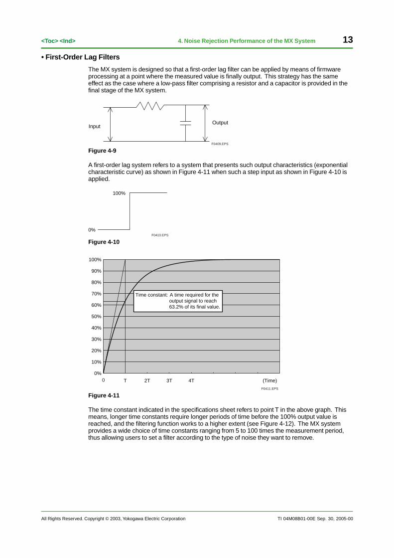
The MX system is designed so that a first-order lag filter can be applied by means of firmwareprocessing at a point where the measured value is finally output. This strategy has the sameeffect as the case where a low-pass filter comprising a resistor and a capacitor is provided in thefinal stage of the MX system.
InputOutput
F0409.EPS
Figure 4-9
A first-order lag system refers to a system that presents such output characteristics (exponentialcharacteristic curve) as shown in Figure 4-11 when such a step input as shown in Figure 4-10 isapplied.
100%
0%F0410.EPS
Figure 4-10
100%
90%
80%
70%
60%
50%
40%
30%
20%
10%
0%
2TT 3T 4T (Time)
Time constant: A time required for the output signal to reach 63.2% of its final value.
0
F0411.EPS
Figure 4-11
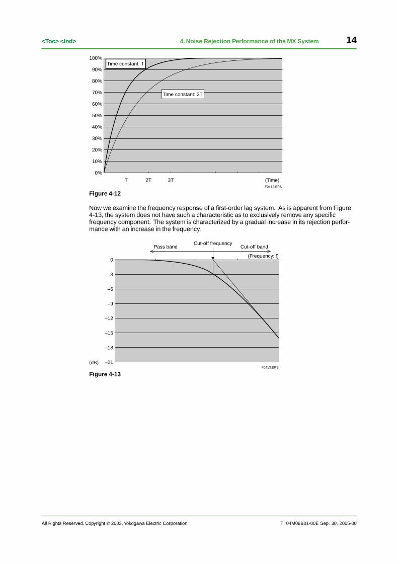
The time constant indicated in the specifications sheet refers to point T in the above graph. Thismeans, longer time constants require longer periods of time before the 100% output value isreached, and the filtering function works to a higher extent (see Figure 4-12). The MX systemprovides a wide choice of time constants ranging from 5 to 100 times the measurement period,thus allowing users to set a filter according to the type of noise they want to remove.
Sep. 30, 2005-00
14
All Rights Reserved. Copyright © 2003, Yokogawa Electric Corporation
<Toc> <Ind>
TI 04M08B01-00E
4. Noise Rejection Performance of the MX System
100%
90%
80%
70%
60%
50%
40%
30%
20%
10%
0%
2TT 3T (Time)
Time constant: T
Time constant: 2T
F0412.EPS
Figure 4-12
Now we examine the frequency response of a first-order lag system. As is apparent from Figure4-13, the system does not have such a characteristic as to exclusively remove any specificfrequency component. The system is characterized by a gradual increase in its rejection perfor-mance with an increase in the frequency.
0
–3
–6
–9
–12
–15
–18
–21
(Frequency: f)
Cut-off bandCut-off frequency
Pass band
F0413.EPS(dB)
Figure 4-13
Sep. 30, 2005-00
All Rights Reserved. Copyright © 2003, Yokogawa Electric Corporation TI 04M08B01-00E
15<Toc> <Ind> 4. Noise Rejection Performance of the MX System
• Tip: Moving Average
In practical applications, Yokogawa considers it sufficiently effective to use both an integrating A/Dconverter and a first-order lag filter in order to achieve noise rejection. For this reason, the MXsystem has no moving average function.
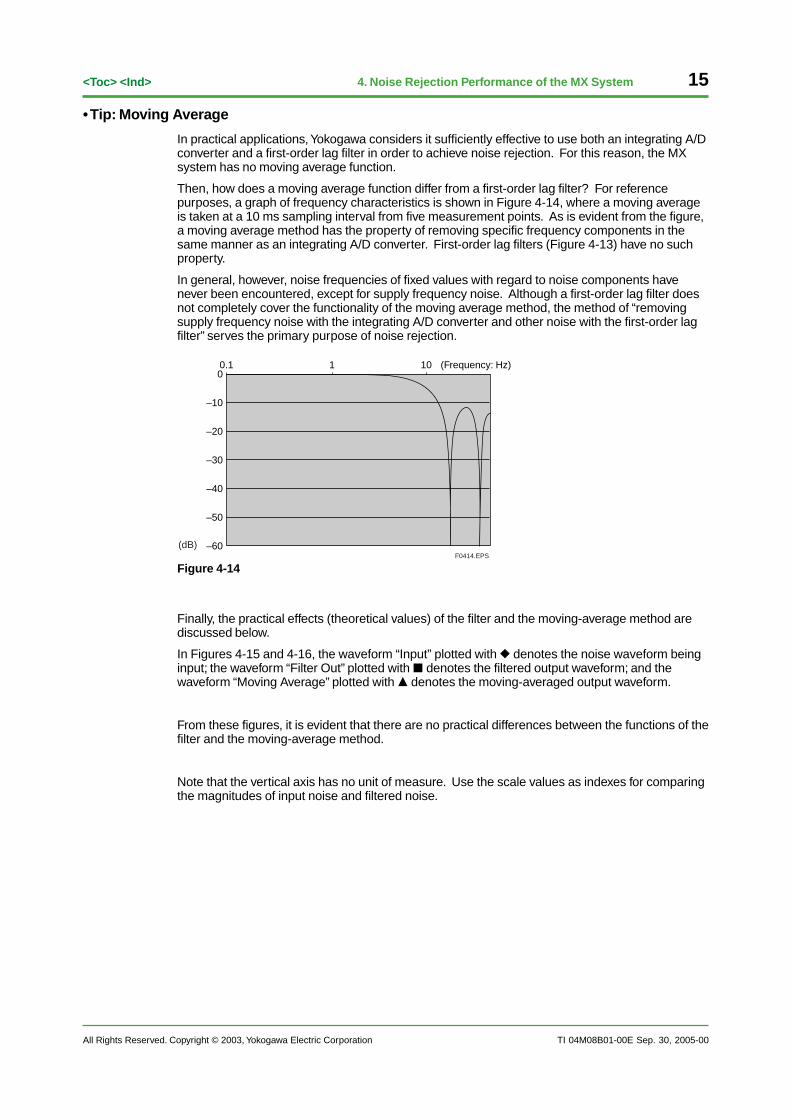
Then, how does a moving average function differ from a first-order lag filter? For referencepurposes, a graph of frequency characteristics is shown in Figure 4-14, where a moving averageis taken at a 10 ms sampling interval from five measurement points. As is evident from the figure,a moving average method has the property of removing specific frequency components in thesame manner as an integrating A/D converter. First-order lag filters (Figure 4-13) have no suchproperty.
In general, however, noise frequencies of fixed values with regard to noise components havenever been encountered, except for supply frequency noise. Although a first-order lag filter doesnot completely cover the functionality of the moving average method, the method of “removingsupply frequency noise with the integrating A/D converter and other noise with the first-order lagfilter” serves the primary purpose of noise rejection.
00.1 1 10
–10
–20
–30
–40
–50
–60
(Frequency: Hz)
F0414.EPS
(dB)
Figure 4-14
Finally, the practical effects (theoretical values) of the filter and the moving-average method arediscussed below.
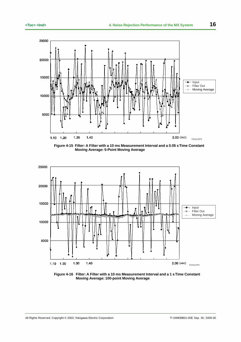
In Figures 4-15 and 4-16, the waveform “Input” plotted with � denotes the noise waveform beinginput; the waveform “Filter Out” plotted with � denotes the filtered output waveform; and thewaveform “Moving Average” plotted with � denotes the moving-averaged output waveform.
From these figures, it is evident that there are no practical differences between the functions of thefilter and the moving-average method.
Note that the vertical axis has no unit of measure. Use the scale values as indexes for comparingthe magnitudes of input noise and filtered noise.
Sep. 30, 2005-00
16
All Rights Reserved. Copyright © 2003, Yokogawa Electric Corporation
<Toc> <Ind>
TI 04M08B01-00E
4. Noise Rejection Performance of the MX System
InputFilter OutMoving Average
F0415.EPS
Figure 4-15 Filter: A Filter with a 10 ms Measurement Interval and a 0.05 s Time Constant Moving Average: 5-Point Moving Average
InputFilter OutMoving Average
F0416.EPS
Figure 4-16 Filter: A Filter with a 10 ms Measurement Interval and a 1 s Time Constant Moving Average: 100-point Moving Average
Sep. 30, 2005-00
All Rights Reserved. Copyright © 2003, Yokogawa Electric Corporation TI 04M08B01-00E
17<Toc> <Ind> 5. Time Stamping of MX System
Sep. 30, 2005-00
5. Time Stamping of MX System• MX System Clock
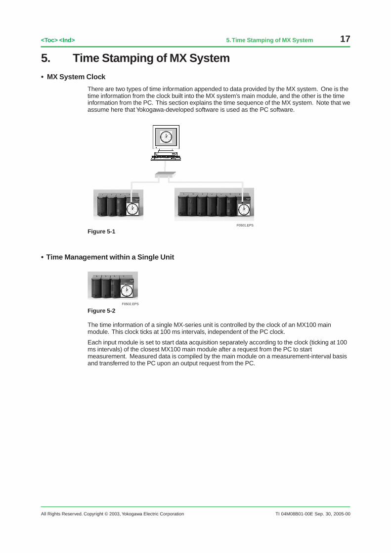
There are two types of time information appended to data provided by the MX system. One is thetime information from the clock built into the MX system’s main module, and the other is the timeinformation from the PC. This section explains the time sequence of the MX system. Note that weassume here that Yokogawa-developed software is used as the PC software.
F0501.EPS
Figure 5-1
• Time Management within a Single Unit
F0502.EPS
Figure 5-2
The time information of a single MX-series unit is controlled by the clock of an MX100 mainmodule. This clock ticks at 100 ms intervals, independent of the PC clock.
Each input module is set to start data acquisition separately according to the clock (ticking at 100ms intervals) of the closest MX100 main module after a request from the PC to startmeasurement. Measured data is compiled by the main module on a measurement-interval basisand transferred to the PC upon an output request from the PC.
18
All Rights Reserved. Copyright © 2003, Yokogawa Electric Corporation
<Toc> <Ind>
TI 04M08B01-00E
5. Time Stamping of MX System
Sep. 30, 2005-00
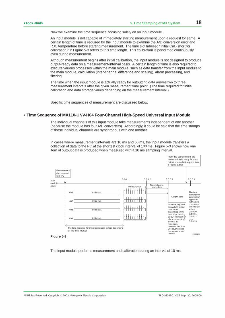
Now we examine the time sequence, focusing solely on an input module.
An input module is not capable of immediately starting measurement upon a request for same. Acertain length of time is required for the input module to examine the A/D conversion error andRJC temperature before starting measurement. The time slot labelled “Initial Cal. (short forcalibration)” in Figure 5-3 refers to this time length. This calibration is performed continuouslyeven during measurement.
Although measurement begins after initial calibration, the input module is not designed to produceoutput-ready data on a measurement-interval basis. A certain length of time is also required toexecute various processes within the main module, such as data transfer from the input module tothe main module, calculation (inter-channel difference and scaling), alarm processing, andfiltering.
The time when the input module is actually ready for outputting data arrives two to threemeasurement intervals after the given measurement time point. (The time required for initialcalibration and data storage varies depending on the measurement interval.)
Specific time sequences of measurement are discussed below.
• Time Sequence of MX110-UNV-H04 Four-Channel High-Speed Universal Input Module
The individual channels of this input module take measurements independent of one another(because the module has four A/D converters). Accordingly, it could be said that the time stampsof these individual channels are synchronous with one another.
In cases where measurement intervals are 10 ms and 50 ms, the input module transfers acollection of data to the PC at the shortest clock interval of 100 ms. Figure 5-3 shows how oneitem of output data is produced when measured with a 10 ms sampling interval.
Measurement start request from PC
The time stamp (time information) appended to this data comprises ten different values: 0:0:0.10, 0:0:0.11, 0:0:0.12, . . . , 0:0:0.19.
The time required to produce output data varies depending on the type of processing (e.g., calculation or alarm processing). Even at its maximum, however, this time will never exceed the measurement interval.
From this point onward, the main module is ready for data output upon a first request from a PC for output
ch1
0:0:0.1 0:0:0.2
Time taken to store dataMeasurement
0:0:0.3 0:0:0.4
Initial cal.
ch2 Initial cal.
ch3 Initial cal.
ch4 Initial cal.
Output data
F0503.EPS
Main module's clock
The time required for initial calibration differs depending on the time interval
Figure 5-3
The input module performs measurement and calibration during an interval of 10 ms.
All Rights Reserved. Copyright © 2003, Yokogawa Electric Corporation TI 04M08B01-00E
19<Toc> <Ind> 5. Time Stamping of MX System
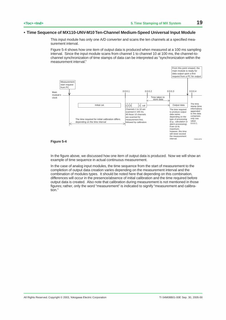
• Time Sequence of MX110-UNV-M10 Ten-Channel Medium-Speed Universal Input Module
This input module has only one A/D converter and scans the ten channels at a specified mea-surement interval.
Figure 5-4 shows how one item of output data is produced when measured at a 100 ms samplinginterval. Since the input module scans from channel 1 to channel 10 at 100 ms, the channel-to-channel synchronization of time stamps of data can be interpreted as “synchronization within themeasurement interval.”
Measurement start request from PC
The time stamp (time information) appended to this data comprises only one value: 0:0:0.1.
Channels 1 to 10 are scanned in 100 ms. All these 10 channels are scanned for measurement first, followed by calibration.
The time required to produce output data varies depending on the type of processing (e.g., calculation or alarm processing). Even at its maximum, however, this time will never exceed the measurement interval.
From this point onward, the main module is ready for data output upon a first request from a PC for output
0:0:0.1 0:0:0.2
Time taken to store data
0:0:0.3 0:0:0.4
Initial cal. Output data1 2 3 10 cal
F0504.EPS
Main module's clock
The time required for initial calibration differs depending on the time interval
Figure 5-4
In the figure above, we discussed how one item of output data is produced. Now we will show anexample of time sequence in actual continuous measurement.
In the case of analog input modules, the time sequence from the start of measurement to thecompletion of output data creation varies depending on the measurement interval and thecombination of modules types. It should be noted here that depending on this combination,differences will occur in the presence/absence of initial calibration and the time required beforeoutput data is created. Also note that calibration during measurement is not mentioned in thosefigures; rather, only the word “measurement” is indicated to signify “measurement and calibra-tion.”
Sep. 30, 2005-00
20
All Rights Reserved. Copyright © 2003, Yokogawa Electric Corporation
<Toc> <Ind>
TI 04M08B01-00E
5. Time Stamping of MX System
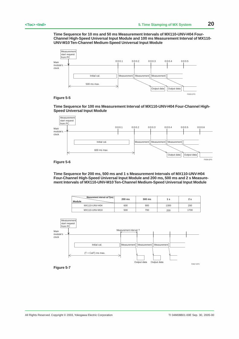
Time Sequence for 10 ms and 50 ms Measurement Intervals of MX110-UNV-H04 Four-Channel High-Speed Universal Input Module and 100 ms Measurement Interval of MX110-UNV-M10 Ten-Channel Medium-Speed Universal Input Module
0:0:0.1 0:0:0.2 0:0:0.3 0:0:0.4 0:0:0.5
Initial cal. Measurement Measurement Measurement
Output data Output data
F0505.EPS
Main module's clock
500 ms max.
Measurement start request from PC
Figure 5-5
Time Sequence for 100 ms Measurement Interval of MX110-UNV-H04 Four-Channel High-Speed Universal Input Module
0:0:0.1 0:0:0.2 0:0:0.3 0:0:0.4 0:0:0.5 0:0:0.6
Initial cal. Measurement Measurement Measurement
Output data Output data
F0506.EPS
Main module's clock
600 ms max.
Measurement start request from PC
Figure 5-6
Time Sequence for 200 ms, 500 ms and 1 s Measurement Intervals of MX110-UNV-H04Four-Channel High-Speed Universal Input Module and 200 ms, 500 ms and 2 s Measure-ment Intervals of MX110-UNV-M10 Ten-Channel Medium-Speed Universal Input Module
1 s500 ms
1300
2 s200 ms
900600 200
200700 1700500
MX110-UNV-H04
MX110-UNV-M10
Measurement interval cal T(ms)
Module
(T + CalT) ms max.
Initial cal. Measurement Measurement Measurement
Measurement interval: T
Output data Output dataF0507.EPS
Main module's clock
Measurement start request from PC
Figure 5-7
Sep. 30, 2005-00
All Rights Reserved. Copyright © 2003, Yokogawa Electric Corporation TI 04M08B01-00E
21<Toc> <Ind> 5. Time Stamping of MX System
Time Sequence for 2 s and Longer Measurement Intervals of MX110-UNV-H04 Four-Channel High-Speed Universal Input Module and 1 s/5 s and Longer MeasurementIntervals of MX110-UNV-M10 Ten-Channel Medium-Speed Universal Input Module
(T + 200) ms max.
Measurement Measurement Measurement
Measurement interval: T
Output data Output data Output data F0508.EPS
Main module's clock
Measurement start request from PC
Figure 5-8
Time Sequence for 10 s, 20 s, 30 s and 60 s Measurement Intervals
(T + 200) ms max.
Measurement
Output data
Measurement
Output data
Measurement
5s
Measurement interval: T
F0509.EPS
Main module's clock
Measurement start request from PC
Figure 5-9
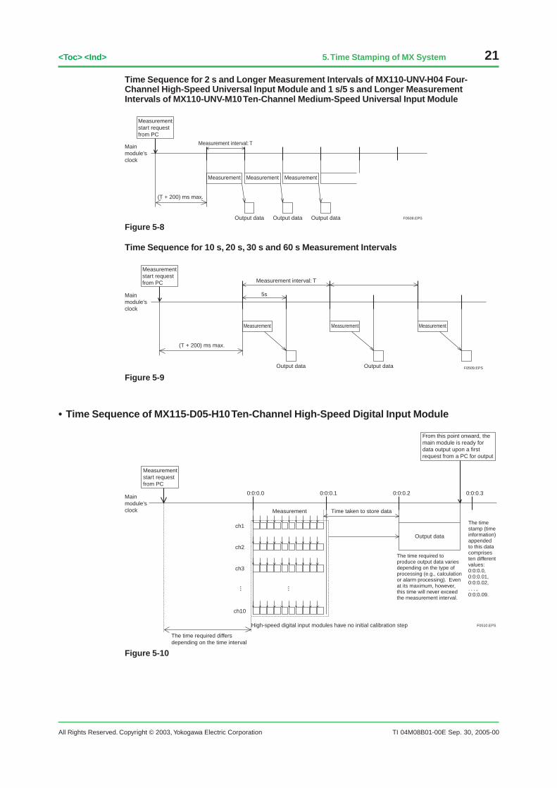
• Time Sequence of MX115-D05-H10 Ten-Channel High-Speed Digital Input Module
Measurement start request from PC
The time stamp (time information) appended to this data comprises ten different values: 0:0:0.0, 0:0:0.01, 0:0:0.02, . . . , 0:0:0.09.
The time required to produce output data varies depending on the type of processing (e.g., calculation or alarm processing). Even at its maximum, however, this time will never exceed the measurement interval.
From this point onward, the main module is ready for data output upon a first request from a PC for output
0:0:0.0 0:0:0.1
Time taken to store data
High-speed digital input modules have no initial calibration step
0:0:0.2 0:0:0.3
Output data
ch1
ch2
ch3
ch10
Measurement
F0510.EPS
Main module's clock
The time required differs depending on the time interval
Figure 5-10
Sep. 30, 2005-00
22
All Rights Reserved. Copyright © 2003, Yokogawa Electric Corporation
<Toc> <Ind>
TI 04M08B01-00E
5. Time Stamping of MX System
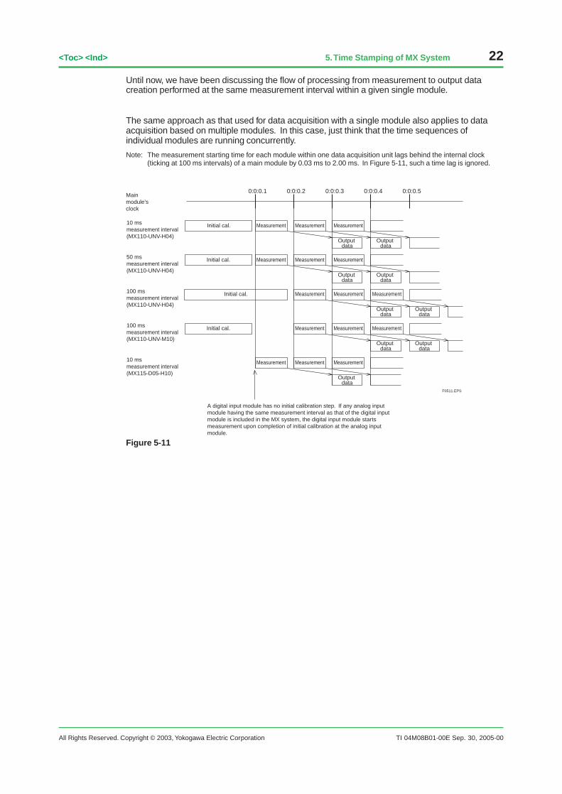
Until now, we have been discussing the flow of processing from measurement to output datacreation performed at the same measurement interval within a given single module.
The same approach as that used for data acquisition with a single module also applies to dataacquisition based on multiple modules. In this case, just think that the time sequences ofindividual modules are running concurrently.
Note: The measurement starting time for each module within one data acquisition unit lags behind the internal clock(ticking at 100 ms intervals) of a main module by 0.03 ms to 2.00 ms. In Figure 5-11, such a time lag is ignored.
10 ms measurement interval(MX110-UNV-H04)
0:0:0.2 0:0:0.3 0:0:0.40:0:0.1 0:0:0.5
Initial cal. Measurement Measurement Measurement
Output data
Output data
50 ms measurement interval(MX110-UNV-H04)
Initial cal. Measurement Measurement Measurement
Output data
Output data
100 ms measurement interval(MX110-UNV-H04)
Initial cal. Measurement Measurement Measurement
Output data
Output data
100 ms measurement interval(MX110-UNV-M10)
Initial cal. Measurement Measurement Measurement
Output data
Output data
10 ms measurement interval(MX115-D05-H10)
Measurement Measurement Measurement
Output data
F0511.EPS
A digital input module has no initial calibration step. If any analog input module having the same measurement interval as that of the digital input module is included in the MX system, the digital input module starts measurement upon completion of initial calibration at the analog input module.
Main module's clock
Figure 5-11
Sep. 30, 2005-00
All Rights Reserved. Copyright © 2003, Yokogawa Electric Corporation TI 04M08B01-00E
23<Toc> <Ind> 5. Time Stamping of MX System
• Inter-channel Calculation
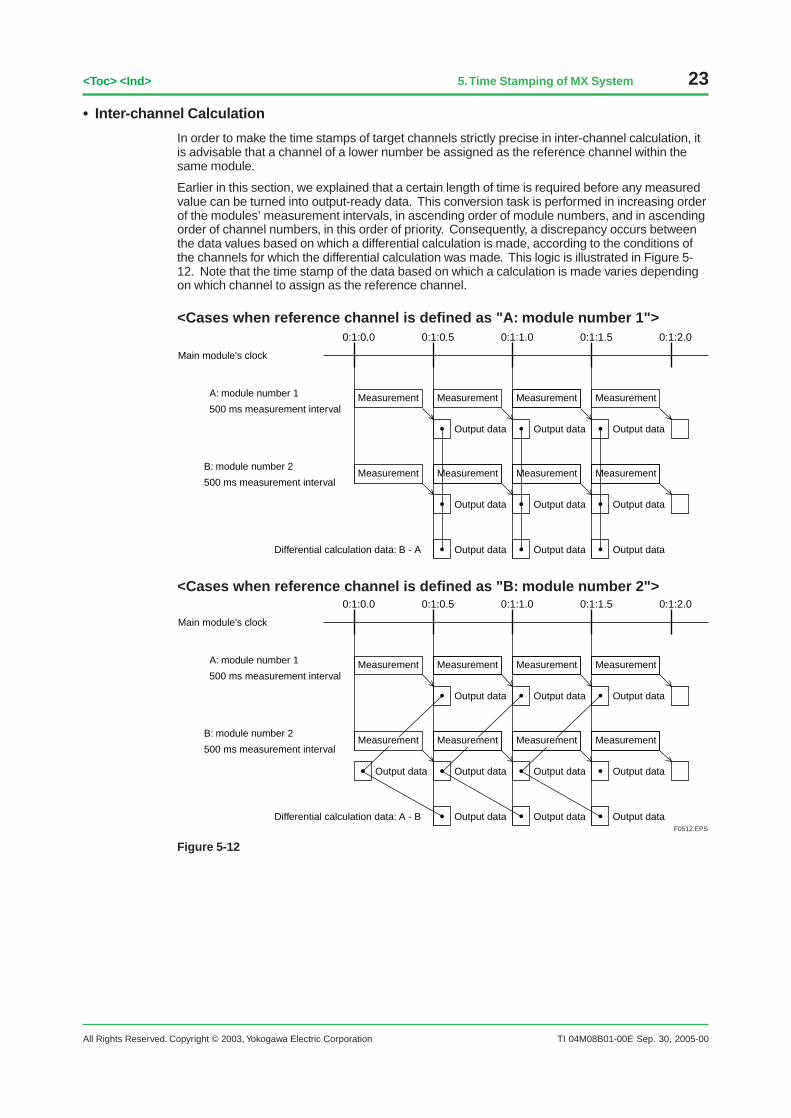
In order to make the time stamps of target channels strictly precise in inter-channel calculation, itis advisable that a channel of a lower number be assigned as the reference channel within thesame module.
Earlier in this section, we explained that a certain length of time is required before any measuredvalue can be turned into output-ready data. This conversion task is performed in increasing orderof the modules’ measurement intervals, in ascending order of module numbers, and in ascendingorder of channel numbers, in this order of priority. Consequently, a discrepancy occurs betweenthe data values based on which a differential calculation is made, according to the conditions ofthe channels for which the differential calculation was made. This logic is illustrated in Figure 5-12. Note that the time stamp of the data based on which a calculation is made varies dependingon which channel to assign as the reference channel.
Main module's clock
A: module number 1
500 ms measurement interval
0:1:2.00:1:1.50:1:1.00:1:0.5
Output data
0:1:0.0
Measurement
B: module number 2
500 ms measurement interval
Differential calculation data: B - A
Output data
Measurement
Output data
Measurement Measurement
Output data
Measurement
Output data
Measurement
Output data
Measurement
Output data Output data Output data
Measurement
Main module's clock
A: module number 1
500 ms measurement interval
0:1:2.00:1:1.50:1:1.00:1:0.5
Output data
0:1:0.0
B: module number 2
500 ms measurement interval
Differential calculation data: A - B
Output data Output data
Output dataOutput data Output data Output data
Output data Output data Output data
Measurement Measurement Measurement Measurement
Measurement Measurement Measurement Measurement
F0512.EPS
<Cases when reference channel is defined as "A: module number 1">
<Cases when reference channel is defined as "B: module number 2">
Figure 5-12
Sep. 30, 2005-00
24
All Rights Reserved. Copyright © 2003, Yokogawa Electric Corporation
<Toc> <Ind>
TI 04M08B01-00E
5. Time Stamping of MX System
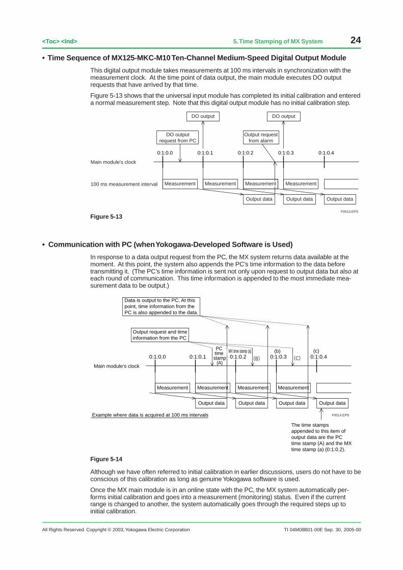
• Time Sequence of MX125-MKC-M10 Ten-Channel Medium-Speed Digital Output Module
This digital output module takes measurements at 100 ms intervals in synchronization with themeasurement clock. At the time point of data output, the main module executes DO outputrequests that have arrived by that time.
Figure 5-13 shows that the universal input module has completed its initial calibration and entereda normal measurement step. Note that this digital output module has no initial calibration step.
Main module's clock
100 ms measurement interval
0:1:0.40:1:0.30:1:0.20:1:0.10:1:0.0
Measurement Measurement Measurement Measurement
Output data Output data Output data
DO output request from PC
Output request from alarm
DO output DO output
F0513.EPS
Figure 5-13
• Communication with PC (when Yokogawa-Developed Software is Used)
In response to a data output request from the PC, the MX system returns data available at themoment. At this point, the system also appends the PC’s time information to the data beforetransmitting it. (The PC’s time information is sent not only upon request to output data but also ateach round of communication. This time information is appended to the most immediate mea-surement data to be output.)
Main module's clock
0:1:0.40:1:0.30:1:0.20:1:0.10:1:0.0
Measurement Measurement Measurement Measurement
Output dataOutput data Output data Output data
Output request and time information from the PC
Data is output to the PC. At this point, time information from the PC is also appended to the data.
Example where data is acquired at 100 ms intervals F0514.EPS
B C
PC time stamp
(A)
MX time stamp (a) (b) (c)
The time stamps appended to this item of output data are the PC time stamp (A) and the MX time stamp (a) (0:1:0.2).
Figure 5-14
Although we have often referred to initial calibration in earlier discussions, users do not have to beconscious of this calibration as long as genuine Yokogawa software is used.
Once the MX main module is in an online state with the PC, the MX system automatically per-forms initial calibration and goes into a measurement (monitoring) status. Even if the currentrange is changed to another, the system automatically goes through the required steps up toinitial calibration.
Sep. 30, 2005-00
All Rights Reserved. Copyright © 2003, Yokogawa Electric Corporation TI 04M08B01-00E
25<Toc> <Ind> 5. Time Stamping of MX System
• Realtime Monitoring Screen (when Yokogawa-Developed Software is Used)
The Realtime Monitoring screen shows data in a visual form according to time information fromthe MX main module, rather than from the PC.
• Viewer Screen (when Yokogawa-Developed Software is Used)
In the case of stored data, however, the time stamp of either the MX main module or the PC canbe chosen to visually replay the data. Then, why is it necessary to show the time information ofthe PC?
Let us consider the following case where data is obtained from two MX units using a single PC.
F0515.EPSUnit A Unit B
Figure 5-15
Suppose the clocks of units A and B are in perfect synchronization with each other. Then, dataacquisition can be achieved by simply relying on time information from the MX units only. Inpractice, however, this synchronization is not possible.
The degree of time disagreement between the MX units depends on their clock accuracy. Theclock accuracy of the MX main module is specified as ±100 ppm. This clock accuracy results in aweekly error of (3600 × 24 × 7)/1000000 × 100 ≈ 60 sec. In other words, in a case where dataacquisition is performed continuously for one week at an interval of one second, the number ofdata items acquired may differ between units A and B to a maximum of 120 items (60 × 2) eventhough the data is acquired over the same period. In order to absorb this difference, the PC clocktime is used to correct the number of data items before they are processed for visual replay.
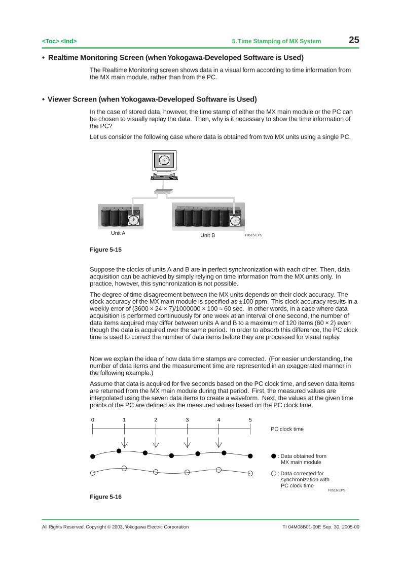
Now we explain the idea of how data time stamps are corrected. (For easier understanding, thenumber of data items and the measurement time are represented in an exaggerated manner inthe following example.)
Assume that data is acquired for five seconds based on the PC clock time, and seven data itemsare returned from the MX main module during that period. First, the measured values areinterpolated using the seven data items to create a waveform. Next, the values at the given timepoints of the PC are defined as the measured values based on the PC clock time.
0 1 2 3 4 5
PC clock time
: Data obtained from MX main module
: Data corrected for synchronization with PC clock time
F0516.EPS
Figure 5-16
Sep. 30, 2005-00
26
All Rights Reserved. Copyright © 2003, Yokogawa Electric Corporation
<Toc> <Ind>
TI 04M08B01-00E
5. Time Stamping of MX System
By applying this process to both units A and B, the data items of these units are caused to holdmeasured values corrected according to the PC clock time. As long as the time axes of theseunits agree with each other, it is possible to draw waveforms spanning the units by properlyarranging these data items.
There is a difference no greater than one measurement interval (100 ms at the shortest) betweenthe PC time stamp appended to the data of the MX units and the time at which the data wasactually sampled. (See the example of Figure 5-14 “Difference between PC Time Stamp (A) andMX Time Stamp (a)”.) However, the time difference between the units is kept smaller than onemeasurement interval (100 ms at the shortest) at any point of time by means of the correctionprocess noted above. Thus, it is possible to visualize data without allowing the time difference toaccumulate.
Sep. 30, 2005-00
All Rights Reserved. Copyright © 2003, Yokogawa Electric Corporation TI 04M08B01-00E
27<Toc> <Ind> 6. Using Strain Conversion Cables (DU450-001)
Sep. 30, 2005-00
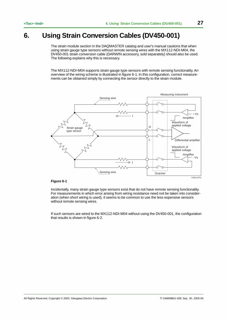
6. Using Strain Conversion Cables (DV450-001)The strain module section in the DAQMASTER catalog and user's manual cautions that whenusing strain gauge type sensors without remote sensing wires with the MX112-NDI-M04, theDV450-001 strain conversion cable (DARWIN accessory, sold separately) should also be used.The following explains why this is necessary.
The MX112-NDI-M04 supports strain gauge type sensors with remote sensing functionality. Anoverview of the wiring scheme is illustrated in figure 6-1. In this configuration, correct measure-ments can be obtained simply by connecting the sensor directly to the strain module.
Sensing wire
Sensing wire
Strain gaugetype sensor
I
I
Measuring instrument
�VsAmplifier
Amplifier
Waveform ofapplied voltage
Waveform ofapplied voltage
Differential amplifier
�Vs
ScannerF0601.EPS
H
L
Figure 6-1
Incidentally, many strain gauge type sensors exist that do not have remote sensing functionality.For measurements in which error arising from wiring resistance need not be taken into consider-ation (when short wiring is used), it seems to be common to use the less expensive sensorswithout remote sensing wires.
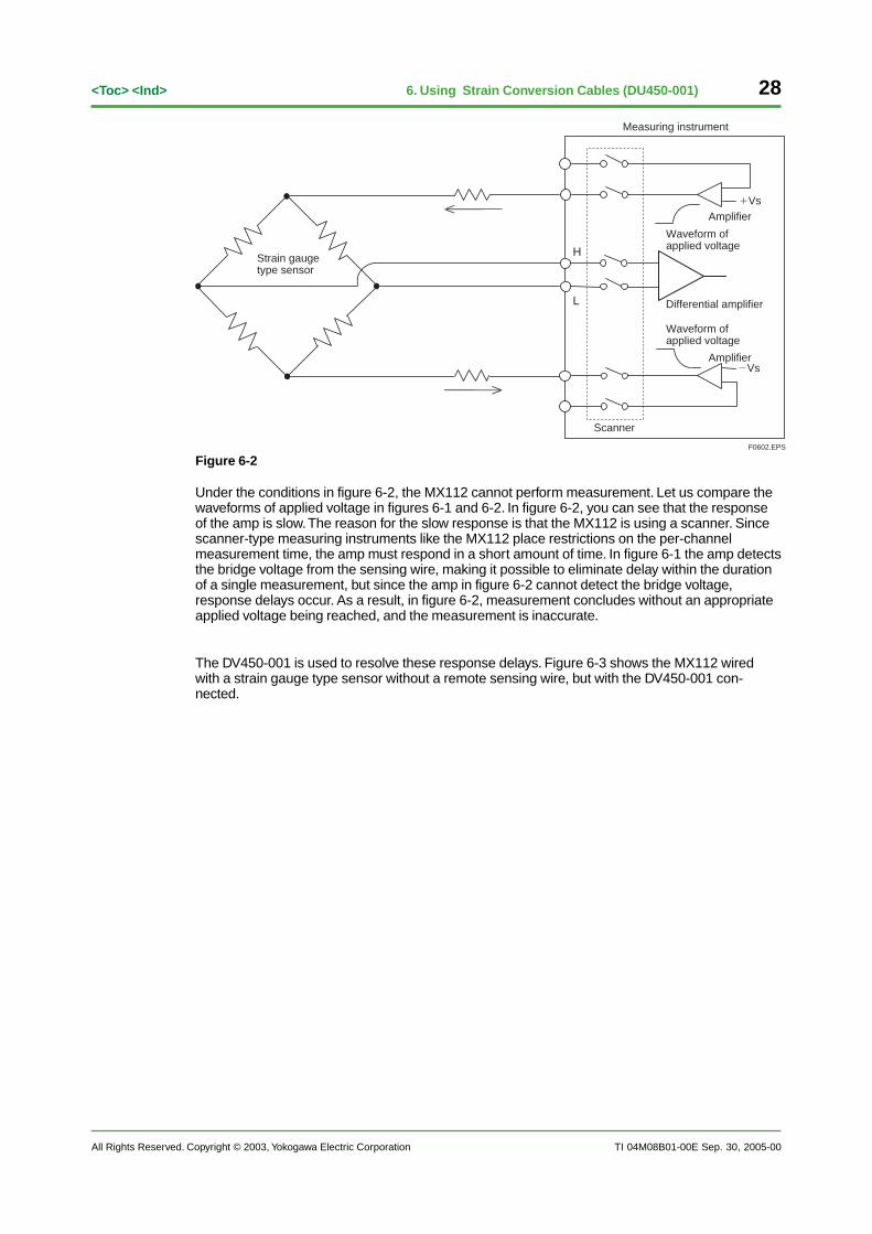
If such sensors are wired to the MX112-NDI-M04 without using the DV450-001, the configurationthat results is shown in figure 6-2.
28
All Rights Reserved. Copyright © 2003, Yokogawa Electric Corporation
<Toc> <Ind>
TI 04M08B01-00E
6. Using Strain Conversion Cables (DU450-001)
F0602.EPS
Strain gaugetype sensor
Measuring instrument
�VsAmplifier
Amplifier
Waveform ofapplied voltage
Waveform ofapplied voltage
Differential amplifier
�Vs
Scanner
H
L
Figure 6-2
Under the conditions in figure 6-2, the MX112 cannot perform measurement. Let us compare thewaveforms of applied voltage in figures 6-1 and 6-2. In figure 6-2, you can see that the responseof the amp is slow. The reason for the slow response is that the MX112 is using a scanner. Sincescanner-type measuring instruments like the MX112 place restrictions on the per-channelmeasurement time, the amp must respond in a short amount of time. In figure 6-1 the amp detectsthe bridge voltage from the sensing wire, making it possible to eliminate delay within the durationof a single measurement, but since the amp in figure 6-2 cannot detect the bridge voltage,response delays occur. As a result, in figure 6-2, measurement concludes without an appropriateapplied voltage being reached, and the measurement is inaccurate.
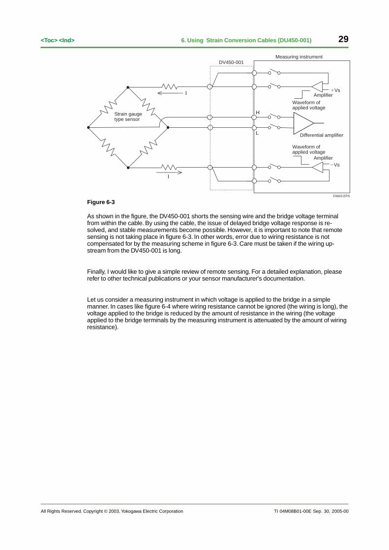
The DV450-001 is used to resolve these response delays. Figure 6-3 shows the MX112 wiredwith a strain gauge type sensor without a remote sensing wire, but with the DV450-001 con-nected.
Sep. 30, 2005-00
All Rights Reserved. Copyright © 2003, Yokogawa Electric Corporation TI 04M08B01-00E
29<Toc> <Ind> 6. Using Strain Conversion Cables (DU450-001)
I
I
F0603.EPS
DV450-001
Strain gaugetype sensor
Measuring instrument
�VsAmplifier
Amplifier
Waveform ofapplied voltage
Waveform ofapplied voltage
Differential amplifier
�Vs
H
L
Figure 6-3
As shown in the figure, the DV450-001 shorts the sensing wire and the bridge voltage terminalfrom within the cable. By using the cable, the issue of delayed bridge voltage response is re-solved, and stable measurements become possible. However, it is important to note that remotesensing is not taking place in figure 6-3. In other words, error due to wiring resistance is notcompensated for by the measuring scheme in figure 6-3. Care must be taken if the wiring up-stream from the DV450-001 is long.
Finally, I would like to give a simple review of remote sensing. For a detailed explanation, pleaserefer to other technical publications or your sensor manufacturer's documentation.
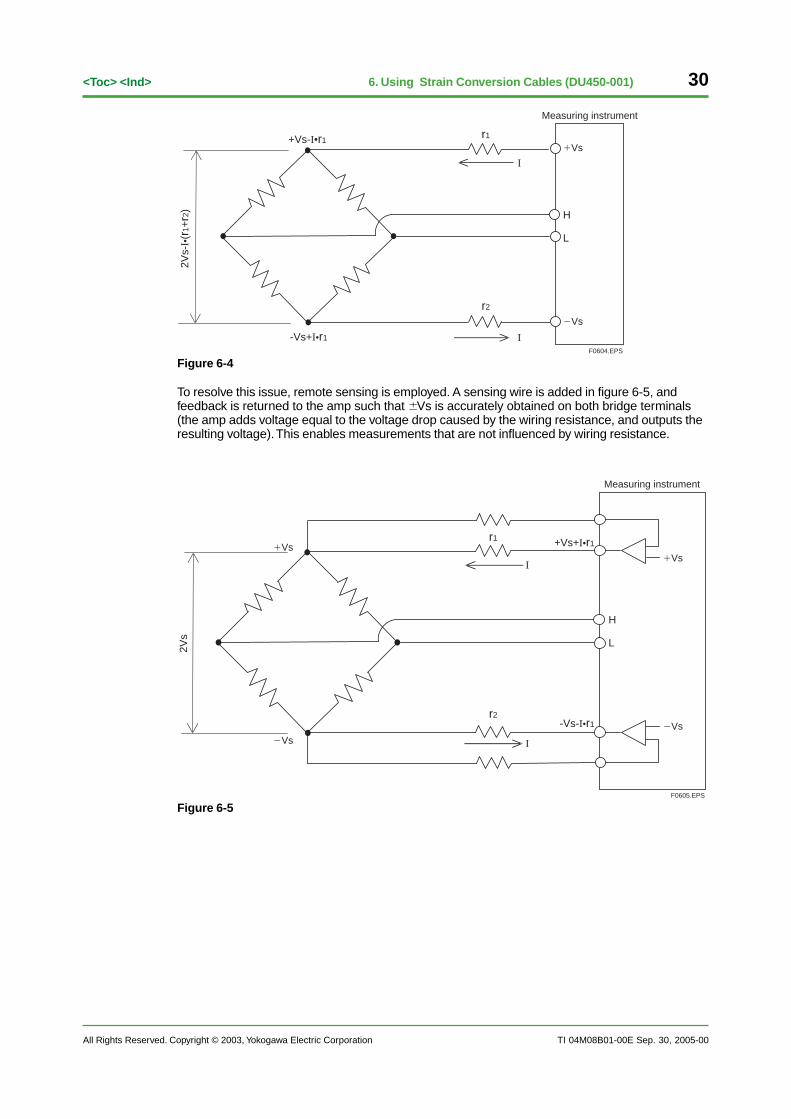
Let us consider a measuring instrument in which voltage is applied to the bridge in a simplemanner. In cases like figure 6-4 where wiring resistance cannot be ignored (the wiring is long), thevoltage applied to the bridge is reduced by the amount of resistance in the wiring (the voltageapplied to the bridge terminals by the measuring instrument is attenuated by the amount of wiringresistance).
Sep. 30, 2005-00
30
All Rights Reserved. Copyright © 2003, Yokogawa Electric Corporation
<Toc> <Ind>
TI 04M08B01-00E
6. Using Strain Conversion Cables (DU450-001)
2Vs-
I•(r
1+r2
)
+Vs-I•r1
-Vs+I•r1
I
IF0604.EPS
r1
r2
Measuring instrument
�Vs
�Vs
H
L
Figure 6-4
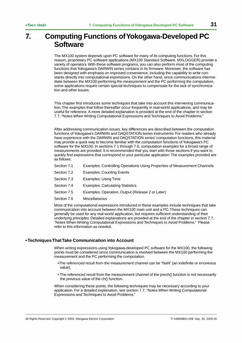
To resolve this issue, remote sensing is employed. A sensing wire is added in figure 6-5, andfeedback is returned to the amp such that � Vs is accurately obtained on both bridge terminals(the amp adds voltage equal to the voltage drop caused by the wiring resistance, and outputs theresulting voltage). This enables measurements that are not influenced by wiring resistance.
2Vs
-Vs-I•r1
+Vs+I•r1
I
I
F0605.EPS
r1
r2
Measuring instrument
�Vs
�Vs
H
L
�Vs
�Vs
Figure 6-5
Sep. 30, 2005-00
All Rights Reserved. Copyright © 2003, Yokogawa Electric Corporation TI 04M08B01-00E
31<Toc> <Ind> 7. Computing Functions of Yokogawa-Developed PC Software
Sep. 30, 2005-00
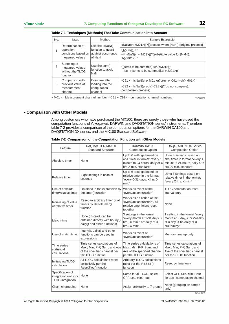
7. Computing Functions of Yokogawa-Developed PCSoftwareThe MX100 system depends upon PC software for many of its computing functions. For thisreason, proprietary PC software applications (MX100 Standard Software, MXLOGGER) provide avariety of operators. With these software programs, you can also perform most of the computingfunctions that Yokogawa’s DARWIN series contains in its firmware. Moreover, the software hasbeen designed with emphasis on improved convenience, including the capability to write con-stants directly into computational expressions. On the other hand, since communications interme-diate between the MX100 performing the measurement and the PC performing the computation,some applications require certain special techniques to compensate for the lack of synchroniza-tion and other issues.
This chapter first introduces some techniques that take into account this intervening communica-tion. The examples that follow thereafter occur frequently in real-world applications, and may beuseful for reference. A more detailed explanation is provided at the end of the chapter in section7.7, “Notes When Writing Computational Expressions and Techniques to Avoid Problems.”
After addressing communication issues, key differences are described between the computationfunctions of Yokogawa’s DARWIN and DAQSTATION series instruments. For readers who alreadyhave experience with the DARWIN and DAQSTATION series’ computation functions, this materialmay provide a quick way to become familiar with the computation functions of Yokogawa’s PCsoftware for the MX100. In sections 7.1 through 7.6, computation examples for a broad range ofmeasurements are provided. It is recommended that you start with those sections if you want toquickly find expressions that correspond to your particular application. The examples provided areas follows:
Section 7.1 Examples: Controlling Operations Using Properties of Measurement Channels
Section 7.2 Examples: Counting Events
Section 7.3 Examples: Using Time
Section 7.4 Examples: Calculating Statistics
Section 7.5 Examples: Operation, Output (Release 2 or Later)
Section 7.6 Miscellaneous
Most of the computational expressions introduced in these examples include techniques that takecommunication into account between the MX100 main unit and a PC. These techniques cangenerally be used for any real-world application, but requires sufficient understanding of theirunderlying principles. Detailed explanations are provided at the end of the chapter in section 7.7,“Notes When Writing Computational Expressions and Techniques to Avoid Problems.” Pleaserefer to this information as needed.
• Techniques That Take Communication into Account
When writing expressions using Yokogawa-developed PC software for the MX100, the followingpoints must be considered since communication is involved between the MX100 performing themeasurement and the PC performing the computation.
•The referenced result from the measurement channel can be “NaN” (an indefinite or erroneousvalue).
• The referenced result from the measurement channel of the prech() function is not necessarilythe previous value of the ch() function.
When considering these points, the following techniques may be necessary according to yourapplication. For a detailed explanation, see section 7.7, “Notes When Writing ComputationalExpressions and Techniques to Avoid Problems.”
32
All Rights Reserved. Copyright © 2003, Yokogawa Electric Corporation
<Toc> <Ind>
TI 04M08B01-00E
7. Computing Functions of Yokogawa-Developed PC Software
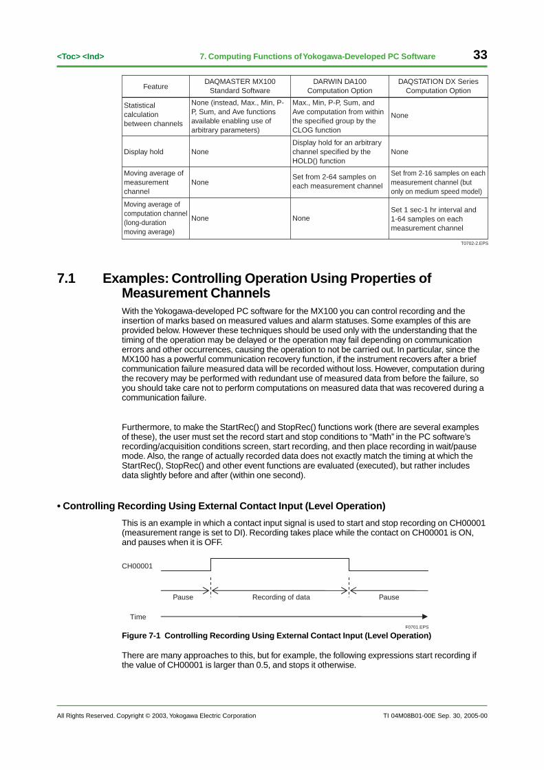
Table 7-1 Techniques (Methods) That Take Communication into Account
T0701.EPS
Use the IsNaN() function to guard against occurrence of NaN
Sample Expression
Use the sum() function to avoid NaN
MethodIssue
Determination of operation conditions based on measured values
Comparison with previous value of measurement channel
Compare after loading into the computation channel
Summing of measured values without the TLOG function
IsNaN(ch(<M01>))?{[process when [NaN]}:{original process}
<C92> = IsNaN(prech(<C91>))?{do not compare}: {comparison process}
<C91> = IsNaN(ch(<M01>))?prech(<C91>):ch(<M01>)
“ch(<M01>)”➝ “(IsNaN(ch(<M01>))?{substitute value for [NaN]}: ch(<M01>))”
No.
“({items to be summed}+ch(<M01>))”➝ “sum({items to be summed},ch(<M01>))”
1
2
3
<M01> = Measurement channel number <C91><C92> = computation channel numbers
• Comparison with Other Models
Among customers who have purchased the MX100, there are surely those who have used thecomputation functions of Yokogawa’s DARWIN and DAQSTATION series’ instruments. Thereforetable 7-2 provides a comparison of the computation options for the DARWIN DA100 andDAQSTATION DX series, and the MX100 Standard Software.
Table 7-2 Comparison of the Computation Function with Other Models
T0702.EPS
Time series calculations of Max., Min, P-P, Sum, and Ave of the specified channel per the TLOG function
Arbitrary TLOG calculations reset per the RESET() function
Works as event of “event/action function”
3 settings in the format “every month at 1-31 days, X hrs., X min.,” or “daily at X hrs., X min.”
Assign arbitrarily to 7 groups
Same for all TLOG, select OFF, sec, min, hour
Works as event of the “event/action function”
DAQSTATION DX Series Computation Option
Up to 3 settings based on abs. timer in format: “every 1 minute to 24 hours, daily at X hrs 00 min. standard”
DARWIN DA100Computation Option
Up to 6 settings based on abs. timer in format: “every 1 minute to 24 hours, daily at X hrs X min. standard”
Up to 6 settings based on relative timer in the format “every 0-31 days, X hrs. X min.”
Works as an action of the “event/action function”, all relative time timers reset together
Reset an arbitrary timer or all timers by ResetTimer() function
DAQMASTER MX100 Standard Software
Obtained in the expression by the timer() function
None
hourly(), daily() and other functions can be used in expressions
Eight settings in units of seconds
None (instead, can be obtained directly with hourly(), daily() and other functions)
Time series calculations of Max., Min, P-P, Sum, and Ave of the specified channel per the TLOG function
None
None
All TLOG calculations reset collectively per the ResetTlog() function
1 setting in the format “every month at X day, X hrs/weekly at X day, X hr./daily at X hrs./hourly”
None (grouping on screen only)
Select OFF, Sec, Min, Hour for each computation channel
Feature
Reset by timer only
TLOG computation reset interval only
Up to 3 settings based on relative timer in the format: “every X hrs. X min.”
None
Memory time up only
Time series calculations of Max., Min, P-P, Sum, and Ave of the specified channel per the TLOG function
Match time
Time series statistical calculations
Initializing of value of relative timer
Use of absolute timer/relative timer
Absolute timer
Relative timer
Use of match time
Channel grouping
Specification of integration units for TLOG integration
Initializing TLOG calculation
Sep. 30, 2005-00
All Rights Reserved. Copyright © 2003, Yokogawa Electric Corporation TI 04M08B01-00E
33<Toc> <Ind> 7. Computing Functions of Yokogawa-Developed PC Software
T0702-2.EPS
DAQSTATION DX Series Computation Option
DARWIN DA100Computation Option
Display hold for an arbitrary channel specified by the HOLD() function
DAQMASTER MX100 Standard Software
Set from 2-64 samples on each measurement channel
None
None
None
Set 1 sec-1 hr interval and1-64 samples on each measurement channel
None
Set from 2-16 samples on each measurement channel (but only on medium speed model)
Feature
None
Moving average of computation channel (long-duration moving average)
Display hold
Moving average of measurement channel
Max., Min, P-P, Sum, and Ave computation from within the specified group by the CLOG function
None (instead, Max., Min, P-P, Sum, and Ave functions available enabling use of arbitrary parameters)
NoneStatistical calculation between channels
7.1 Examples: Controlling Operation Using Properties ofMeasurement ChannelsWith the Yokogawa-developed PC software for the MX100 you can control recording and theinsertion of marks based on measured values and alarm statuses. Some examples of this areprovided below. However these techniques should be used only with the understanding that thetiming of the operation may be delayed or the operation may fail depending on communicationerrors and other occurrences, causing the operation to not be carried out. In particular, since theMX100 has a powerful communication recovery function, if the instrument recovers after a briefcommunication failure measured data will be recorded without loss. However, computation duringthe recovery may be performed with redundant use of measured data from before the failure, soyou should take care not to perform computations on measured data that was recovered during acommunication failure.
Furthermore, to make the StartRec() and StopRec() functions work (there are several examplesof these), the user must set the record start and stop conditions to “Math” in the PC software’srecording/acquisition conditions screen, start recording, and then place recording in wait/pausemode. Also, the range of actually recorded data does not exactly match the timing at which theStartRec(), StopRec() and other event functions are evaluated (executed), but rather includesdata slightly before and after (within one second).
• Controlling Recording Using External Contact Input (Level Operation)
This is an example in which a contact input signal is used to start and stop recording on CH00001(measurement range is set to DI). Recording takes place while the contact on CH00001 is ON,and pauses when it is OFF.
CH00001
Time
Pause PauseRecording of data
F0701.EPS
Figure 7-1 Controlling Recording Using External Contact Input (Level Operation)
There are many approaches to this, but for example, the following expressions start recording ifthe value of CH00001 is larger than 0.5, and stops it otherwise.
Sep. 30, 2005-00
34
All Rights Reserved. Copyright © 2003, Yokogawa Electric Corporation
<Toc> <Ind>
TI 04M08B01-00E
7. Computing Functions of Yokogawa-Developed PC Software
CH99001 = IsNaN(ch(1))?0:ch(1)>0.5?StartRec():StopRec() (7.1)
or
CH99001 = (IsNaN(ch(1))?0:ch(1))>0.5?StartRec():StopRec() (7.2)
The IsNaN() function is used initially in both expressions 7.1 and 7.2; this is a technique that takescommunication into account. It reflects the fact that in expression 7.1 the value of CH00001 canbe NaN, and if it is NaN, nothing is done. In expression 7.2, if the value of CH00001 is NaN, itregards this as 0 and carries out the process under that assumption. When comparing these totable 7-1 in the beginning of this chapter “Techniques Taking Communication into Account,” youcan see that this is an example of one of the techniques introduced.
As an aside, both expressions 7.1 and 7.2 are continuously evaluated as StartRec() being ONwhile contact is ON and StopRec() being OFF while contact is OFF. In principle, you would needan expression that detects the change from ON to OFF or OFF to ON, but in actuality, if theinstrument is already in the state indicated by the function (recording or not recording), thatfunction is not executed. Therefore, it is acceptable to use the expressions in this way.
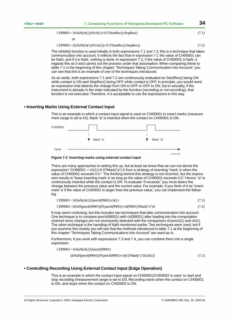
• Inserting Marks Using External Contact Input
This is an example in which a contact input signal is used on CH00001 to insert marks (measure-ment range is set to DI). Mark “a” is inserted when the contact on CH00001 is ON.
CH00001
Mark “a” Mark “a”
TimeF0702.EPS
Figure 7-2 Inserting marks using external contact input
There are many approaches to setting this up, but at least we know that we can not derive theexpression “CH99001 = ch(1)>0.5?Mark(“a”):0 from a strategy of inserting “mark ‘a’ when thevalue of CH00001 exceeds 0.5.” The thinking behind this strategy is not incorrect, but the expres-sion results in “keep inserting mark ‘a’ as long as the value of CH00001 exceeds 0.5.” Hence, “a” iscontinuously inserted while the contact is ON. To evaluate “if exceeds,” you must detect thechange between the previous value and the current value. For example, if you think of it as “insertmark ‘a’ if the value of CH00001 is larger than the previous value,” you can implement the follow-ing.
CH99001 = IsNaN(ch(1))?prech(99001):ch(1) (7.3)
CH99002 = IsNaN(prech(99001))?0:prech(99001)<ch(99001)?Mark(“a”):0 (7.4)
It may seem confusing, but this includes two techniques that take communication into account.One technique is to compare prech(99001) with ch(99001) after loading into the computationchannel since changes are not necessarily detected with the comparison of prech(1) and ch(1).The other technique is the handling of NaN mentioned earlier. Two techniques were used, but ifyou examine this closely you will see that the methods introduced in table 7-1 at the beginning ofthis chapter “Techniques Taking Communications into Account” are used as-is.
Furthermore, if you work with expressions 7.3 and 7.4, you can combine them into a singleexpression.
CH99001 = IsNaN(ch(1))?prech(99001)
:(IsNaN(prech(99001))?0:prech(99001)<ch(1)?Mark(“a”):0,ch(1)) (7.5)
• Controlling Recording Using External Contact Input (Edge Operation)
This is an example in which the contact input signal on CH00001/CH00002 is used to start andstop recording (measurement range is set to DI). Recording starts when the contact on CH00001is ON, and stops when the contact on CH00002 is ON.
Sep. 30, 2005-00
All Rights Reserved. Copyright © 2003, Yokogawa Electric Corporation TI 04M08B01-00E
35<Toc> <Ind> 7. Computing Functions of Yokogawa-Developed PC Software
CH00001
CH00002
Time
Pause PauseRecording of data
F0703.EPS
Figure 7-3 Controlling Recording Using Trigger Input (Edge Operation)
You can set this up using the same method introduced above in “Inserting Marks Using ExternalContact Input.”
If you start with expression 7.5, the following can be derived.
CH99001 = IsNaN(ch(1))?prech(99001)
:(IsNaN(prech(99001))?0:prech(99001)<ch(1)?StartRec():0,ch(1)) (7.6)
CH99002 = IsNaN(ch(2))?prech(99002)
:(IsNaN(prech(99002))?0:prech(99002)<ch(2)?StopRec():0,ch(2)) (7.7)
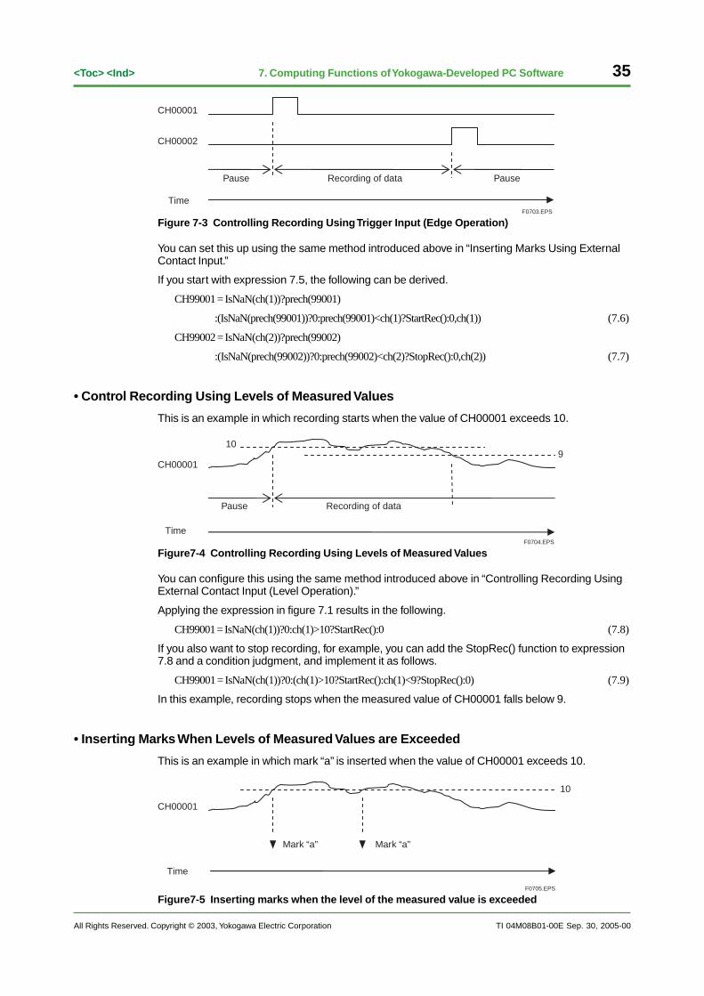
• Control Recording Using Levels of Measured Values
This is an example in which recording starts when the value of CH00001 exceeds 10.
CH00001
10
TimeF0704.EPS
9
Pause Recording of data
Figure7-4 Controlling Recording Using Levels of Measured Values
You can configure this using the same method introduced above in “Controlling Recording UsingExternal Contact Input (Level Operation).”
Applying the expression in figure 7.1 results in the following.
CH99001 = IsNaN(ch(1))?0:ch(1)>10?StartRec():0 (7.8)
If you also want to stop recording, for example, you can add the StopRec() function to expression7.8 and a condition judgment, and implement it as follows.
CH99001 = IsNaN(ch(1))?0:(ch(1)>10?StartRec():ch(1)<9?StopRec():0) (7.9)
In this example, recording stops when the measured value of CH00001 falls below 9.
• Inserting Marks When Levels of Measured Values are Exceeded
This is an example in which mark “a” is inserted when the value of CH00001 exceeds 10.
CH00001
10
Mark “a” Mark “a”
Time
F0705.EPS
Figure7-5 Inserting marks when the level of the measured value is exceeded
Sep. 30, 2005-00
36
All Rights Reserved. Copyright © 2003, Yokogawa Electric Corporation
<Toc> <Ind>
TI 04M08B01-00E
7. Computing Functions of Yokogawa-Developed PC Software
The example is similar to recording control using levels of measured values introduced above, butunlike 7.8 you can apply the same usage as in the above, “Inserting Marks Using ExternalContact Input” (see the preceding explanation for the reasoning used). Apply expression 7-5 andyou can set the condition as “previous reference value is under ten and current reference value isover 10” such that the following results.
CH99001 = IsNaN(ch(1))?prech(99001)
:(IsNaN(prech(99001))?0:(prech(99001)<10)&&(ch(1)>=10)?Mark(“a”):0,ch(1)) (7.10)
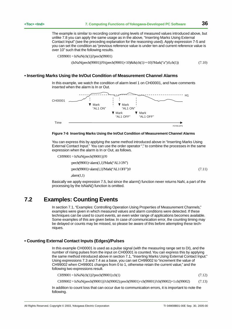
• Inserting Marks Using the In/Out Condition of Measurement Channel Alarms
In this example, we watch the condition of alarm level 1 on CH00001, and have commentsinserted when the alarm is In or Out.
CH00001
H1
Mark“AL1 ON”
Mark“AL1 ON”
Mark“AL1 OFF”
Mark“AL1 OFF”
TimeF0706.EPS
Figure 7-6 Inserting Marks Using the In/Out Condition of Measurement Channel Alarms
You can express this by applying the same method introduced above in “Inserting Marks UsingExternal Contact Input.” You can use the order operator “,” to combine the processes in the sameexpression when the alarm is In or Out, as follows.
CH99001 = IsNaN(prech(99001))?0
:prech(99001)<alarm(1,1)?Mark(“AL1 ON”)
:prech(99001)>alarm(1,1)?Mark(“AL1 OFF”):0 (7.11)
,alarm(1,1)
Basically we apply expression 7.5, but since the alarm() function never returns NaN, a part of theprocessing by the IsNaN() function is omitted.
7.2 Examples: Counting EventsIn section 7.1, “Examples: Controlling Operation Using Properties of Measurement Channels,”examples were given in which measured values and alarm conditions were detected. If thesetechniques can be used to count events, an even wider range of applications becomes available.Some examples of this are given below. In case of communication error, the counting timing maybe delayed or counts may be missed, so please be aware of this before attempting these tech-niques.
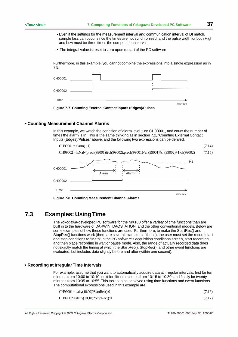
• Counting External Contact Inputs (Edges)/Pulses
In this example CH00001 is used as a pulse signal (with the measuring range set to DI), and thenumber of rising pulses from the input on CH00001 is counted. You can express this by applyingthe same method introduced above in section 7.1, “Inserting Marks Using External Contact Input.”Using expressions 7.3 and 7.4 as a base, you can set CH99002 to “increment the value ofCH99002 when CH99001 changes from 0 to 1, otherwise retain the current value,” and thefollowing two expressions result.
CH99001 = IsNaN(ch(1))?prech(99001):ch(1) (7.12)
CH99002 = IsNaN(prech(99001))?ch(99002):prech(99001)<ch(99001)?ch(99002)+1:ch(99002) (7.13)
In addition to count loss that can occur due to communication errors, it is important to note thefollowing.
Sep. 30, 2005-00
All Rights Reserved. Copyright © 2003, Yokogawa Electric Corporation TI 04M08B01-00E
37<Toc> <Ind> 7. Computing Functions of Yokogawa-Developed PC Software
• Even if the settings for the measurement interval and communication interval of DI match,sample loss can occur since the times are not synchronized, and the pulse width for both Highand Low must be three times the computation interval.
• The integral value is reset to zero upon restart of the PC software
Furthermore, in this example, you cannot combine the expressions into a single expression as in7.5.
CH00001
CH99002
TimeF0707.EPS
Figure 7-7 Counting External Contact Inputs (Edges)/Pulses
• Counting Measurement Channel Alarms
In this example, we watch the condition of alarm level 1 on CH00001, and count the number oftimes the alarm is In. This is the same thinking as in section 7.2, “Counting External ContactInputs (Edges)/Pulses” above, and the following two expressions can be derived.
CH99001 = alarm(1,1) (7.14)
CH99002 = IsNaN(prech(99001))?ch(99002):prech(99001)<ch(99001)?ch(99002)+1:ch(99002) (7.15)
CH00001
H1
CH99002
TimeF0708.EPS
Alarm Alarm
Figure 7-8 Counting Measurement Channel Alarms
7.3 Examples: Using TimeThe Yokogawa-developed PC software for the MX100 offer a variety of time functions than arebuilt in to the hardware of DARWIN, DAQSTATION, and the other conventional models. Below aresome examples of how these functions are used. Furthermore, to make the StartRec() andStopRec() functions work (there are several examples of these), the user must set the record startand stop conditions to “Math” in the PC software’s acquisition conditions screen, start recording,and then place recording in wait or pause mode. Also, the range of actually recorded data doesnot exactly match the timing at which the StartRec(), StopRec(), and other event functions areevaluated, but includes data slightly before and after (within one second).
• Recording at Irregular Time Intervals
For example, assume that you want to automatically acquire data at irregular intervals, first for tenminutes from 10:00 to 10:10, next for fifteen minutes from 10:15 to 10:30, and finally for twentyminutes from 10:35 to 10:55. This task can be achieved using time functions and event functions.The computational expressions used in this example are:
CH99001 = daily(10,00)?StartRec():0 (7.16)
CH99002 = daily(10,10)?StopRec():0 (7.17)
Sep. 30, 2005-00
38
All Rights Reserved. Copyright © 2003, Yokogawa Electric Corporation
<Toc> <Ind>
TI 04M08B01-00E
7. Computing Functions of Yokogawa-Developed PC Software
CH99003 = daily(10,15)?StartRec():0 (7.18)
CH99004 = daily(10,30)?StopRec():0 (7.19)
CH99005 = daily(10,35)?StartRec():0 (7.20)
CH99006 = daily(10,55)?StopRec():0 (7.21)
These can be used as-is, but as explained in section 7.1, “Controlling Recording Using ExternalContact Input (Level Operation),” considering that it is acceptable to use the StartRec() functionand StopRec() function for level operations, if you set it up as “start or stop recording whenbetween 10:00-10:10, 10:15-10:30, or 10:35-10:55,” then you can reduce the number of expres-sions as follows.
CH99001 = daily(10,0,10,10)||daily(10,15,10,30)||daily(10,35,10,55)?StartRec():StopRec() (7.22)
• Split Files at Specified Times
In such cases as when you want to match up one file’s time range with that of a work shift, thereare instances where you want to split continuously recorded data files at specified times. Whenusing DAQWORX MXLOGGER, depending on the logging conditions that are set, you canspecify “split files daily at XX hrs XX min XX sec” but this does not allow you to specify multipletimes within a single day. And on the MX100 Standard Software, you cannot even make such aspecification at all. You can overcome these limitations by using computational expressions. Forexample, you can split files daily at 7:00, 15:00, and 23:00 with the following expression.
CH99001 = daily(7,0)||daily(15,0)||daily(23,0)?SplitRec():0 (7.23)
• Recording Only during the Daytime from Monday to Friday, and in the Morning on Saturday
Let us assume that you want to record only on weekdays 8:00-17:00 and Saturdays 8:00-12:00.Unfortunately the system cannot identify holidays, so you would need to express this as “IfMonday through Friday and 8:00 to 17:00, or Saturday and 8:00 to 12:00...”
CH99001 =(weekly(1,0,0,6,0,0)&&daily(8,0,17,0))||(weekly(6,0,0,0,0,0)&&daily(8,0,12,0))?StartRec():StopRec()
(7.24)
7.4 Examples: Calculating StatisticsThe statistical calculations built in to the hardware of conventional models differ from product toproduct, but generally time series and between-channel statistics are included. With theYokogawa-developed PC software for the MX100, the TLOG function is available for implementingtime series statistical calculations, but the way of using this differs slightly from the hardwarebased method. This section introduces several examples that take these differences into account.
• Summation Using the TLOG Function
Let us take a simple and practical example in which an amount of flow (L/min) on CH00001 issummed, and reset every hour on the hour. The differences from the conventional model hard-ware computation that need to be paid attention to are as follows.
• Since there is no absolute timer, the time function of the computation function is used.
• Since there is no processing function for the units of summation, a constant multiplier is usedto account for the relationship to the computation interval.
• Reset is performed collectively for all TLOG computations, so when multiple time seriesstatistical processes of differing reset intervals are required, the TLOG function cannot beused.
The resulting computation is shown below when the computation interval is 100 msec and there isonly this one TLOG computation. In expression 7.26, the TLOG computation resets every hour on
Sep. 30, 2005-00
All Rights Reserved. Copyright © 2003, Yokogawa Electric Corporation TI 04M08B01-00E
39<Toc> <Ind> 7. Computing Functions of Yokogawa-Developed PC Software
the hour. In expression 7.27, after the summation of CH0001 by the tlogsum() function, the unitsof summation change from “each minute” to “every 100 msec.” CH99002 is the summed value.
CalcInt = 0.1 (7.25)
CH99001 = hourly(0)?ResetTLog():0 (7.26)
CH99002 = tlogsum(1)/60*CalcInt (7.27)
Summation can be performed in the manner above, but from a practical standpoint the “LowCut”line below is generally used to remove the effects of noise around zero of the output from the flowsensor (converter). In this example, the LowCut point is set at 4 L/min. CH99003 is the summedvalue.
CalcInt = 0.1 (7.28)
LowCut = 4 (7.29)
CH99001 = ch(1)<LowCut?0:ch(1) (7.30)
CH99002 = hourly(0)?ResetTLog():0 (7.31)
CH99003 = tlogsum(99001)/60*CalcInt (7.32)
Furthermore, since the TLOG computation is executed at the interval of the channel underconsideration, if that channel’s interval differs, the statistics will be imprecise. In this example, ifCH00001’s sampling interval is 10 msec, in expression 7.27 the TLOG computation executed atan interval of 10 msec is referenced at 100 msec, but in expression 7.32 the TLOG computationitself is executed at an interval of 100 msec. Please be aware of this.
• Summation without the TLOG Function
In the example above, “Summation Using the TLOG Function,” we can also perform the calcula-tion without the TLOG function. Since we cannot rely on the ResetTLog() function, we set up theexpressions such that they switch between adding to the previous value or adding to 0 dependingon the condition of the time function. The CH99002 below is the summed value.
CalcInt = 0.1 (7.33)
LowCut = 4 (7.34)
CH99001 = ch(1)<LowCut?0:ch(1) (7.35)
CH99002 = sum(ch(99003)?0:ch(99002),ch(99001)/60*CalcInt) (7.36)
CH99003 = hourly(0) (7.37)
The use of the arithmetic function sum() in expression 7.36 is an example of a technique takingcommunication into account as introduced in table 7-1 in the beginning of this chapter. However,in expression 7.35, CH99001 can never be NaN, so actually it is acceptable to use a simple “+”operator for the addition without having to use the sum() function. However, if expression 7.35 iswritten as “CH99001 = ch(1) >= LowCut?ch(1):0”, even if it looks the same, CH99001 can some-times be NaN, so problems can occur if you do not use the sum() function. Furthermore, the factthat the summation is written prior to the time function reference is because the reset timing isdelayed by one interval relative to the operation of the time function, which means that it is resetimmediately after every hour.
• Time Series Averaging without the TLOG Function
When the TLOG function can be used, it is applied in the same manner as in the example above,“Summation Using the TLOG Function.” However if the TLOG function cannot be used, you mustwrite your own “averaging” expression. Specifically, you would calculate the sum and number ofthe time series data then perform division, but if the referenced value from the measurementchannel is NaN, since the sum() function skips this value when performing the summation, thenumber of statistical data will differ from the number of actual computations, so you must bewatchful of this.
An example in which the average temperature on CH00001 is calculated and reset every hour onthe hour is worked out below. Furthermore, in expression 7.39, the logic of the IsNaN() function “IfCH00001 is NaN, 1, otherwise 0” is reversed using the negation operator “!” (in other words, “if
Sep. 30, 2005-00
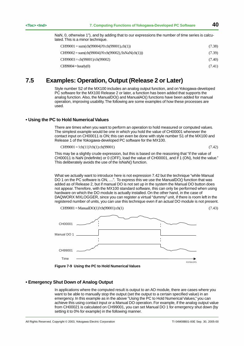
40
All Rights Reserved. Copyright © 2003, Yokogawa Electric Corporation
<Toc> <Ind>
TI 04M08B01-00E
7. Computing Functions of Yokogawa-Developed PC Software
NaN, 0, otherwise 1”), and by adding that to our expressions the number of time series is calcu-lated. This is a minor technique.
CH99001 = sum(ch(99004)?0:ch(99001),ch(1)) (7.38)
CH99002 = sum(ch(99004)?0:ch(99002),!IsNaN(ch(1))) (7.39)
CH99003 = ch(99001)/ch(99002) (7.40)
CH99004 = hourly(0) (7.41)
7.5 Examples: Operation, Output (Release 2 or Later)Style number S2 of the MX100 includes an analog output function, and on Yokogawa-developedPC software for the MX100 Release 2 or later, a function has been added that supports theanalog function. Also, the ManualDO() and ManualAO() functions have been added for manualoperation, improving usability. The following are some examples of how these processes areused.
• Using the PC to Hold Numerical Values
There are times when you want to perform an operation to hold measured or computed values.The simplest example would be one in which you hold the value of CH00001 whenever thecontact input on CH00011 is ON; this can even be done with style number S1 of the MX100 andRelease 1 of the Yokogawa-developed PC software for the MX100.
CH99001 = !ch(11)?ch(1):ch(99001) (7.42)
This may be a slightly crude expression, but this is based on the reasoning that “if the value ofCH00011 is NaN (indefinite) or 0 (OFF), load the value of CH00001, and if 1 (ON), hold the value.”This deliberately avoids the use of the IsNaN() function.
What we actually want to introduce here is not expression 7.42 but the technique “while ManualDO 1 on the PC software is ON, ....”. To express this we use the ManualDO() function that wasadded as of Release 2, but if manual DO is not set up in the system the Manual DO button doesnot appear. Therefore, with the MX100 standard software, this can only be performed when usinghardware on which the DO module is actually installed. On the other hand, in the case ofDAQWORX MXLOGGER, since you can register a virtual “dummy” unit, if there is room left in theregistered number of units, you can use this technique even if an actual DO module is not present.
CH99001 = ManualDO(1)?ch(99001):ch(1) (7.43)
CH00001
CH99001
Manual DO 1
TimeF0709.EPS
Figure 7-9 Using the PC to Hold Numerical Values
• Emergency Shut Down of Analog Output
In applications where the computed result is output to an AO module, there are cases where youwant to be able to manually stop the output (set the output to a certain specified value) in anemergency. In this example as in the above “Using the PC to Hold Numerical Values,” you canachieve this using contact input or a Manual DO operation. For example, if the analog output valuefrom CH00021 is calculated on CH99001, you can set Manual DO 1 for emergency shut down (bysetting it to 0% for example) in the following manner.
Sep. 30, 2005-00
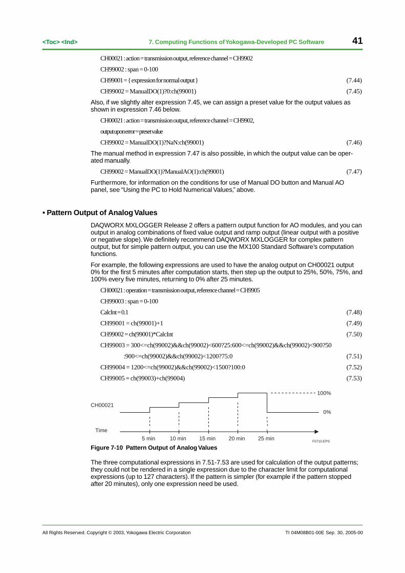
All Rights Reserved. Copyright © 2003, Yokogawa Electric Corporation TI 04M08B01-00E
41<Toc> <Ind> 7. Computing Functions of Yokogawa-Developed PC Software
CH00021 : action = transmission output, reference channel = CH9902
CH99002 : span = 0-100
CH99001 = { expression for normal output } (7.44)
CH99002 = ManualDO(1)?0:ch(99001) (7.45)
Also, if we slightly alter expression 7.45, we can assign a preset value for the output values asshown in expression 7.46 below.
CH00021 : action = transmission output, reference channel = CH9902,
output upon error = preset value
CH99002 = ManualDO(1)?NaN:ch(99001) (7.46)
The manual method in expression 7.47 is also possible, in which the output value can be oper-ated manually.
CH99002 = ManualDO(1)?ManualAO(1):ch(99001) (7.47)
Furthermore, for information on the conditions for use of Manual DO button and Manual AOpanel, see “Using the PC to Hold Numerical Values,” above.
• Pattern Output of Analog Values
DAQWORX MXLOGGER Release 2 offers a pattern output function for AO modules, and you canoutput in analog combinations of fixed value output and ramp output (linear output with a positiveor negative slope). We definitely recommend DAQWORX MXLOGGER for complex patternoutput, but for simple pattern output, you can use the MX100 Standard Software’s computationfunctions.
For example, the following expressions are used to have the analog output on CH00021 output0% for the first 5 minutes after computation starts, then step up the output to 25%, 50%, 75%, and100% every five minutes, returning to 0% after 25 minutes.
CH00021 : operation = transmission output, reference channel = CH9905
CH99003 : span = 0-100
CalcInt = 0.1 (7.48)
CH99001 = ch(99001)+1 (7.49)
CH99002 = ch(99001)*CalcInt (7.50)
CH99003 = 300<=ch(99002)&&ch(99002)<600?25:600<=ch(99002)&&ch(99002)<900?50
:900<=ch(99002)&&ch(99002)<1200?75:0 (7.51)
CH99004 = 1200<=ch(99002)&&ch(99002)<1500?100:0 (7.52)
CH99005 = ch(99003)+ch(99004) (7.53)
CH00021
100%
0%
Time
10 min 15 min 20 min 25 min5 minF0710.EPS
Figure 7-10 Pattern Output of Analog Values
The three computational expressions in 7.51-7.53 are used for calculation of the output patterns;they could not be rendered in a single expression due to the character limit for computationalexpressions (up to 127 characters). If the pattern is simpler (for example if the pattern stoppedafter 20 minutes), only one expression need be used.
Sep. 30, 2005-00
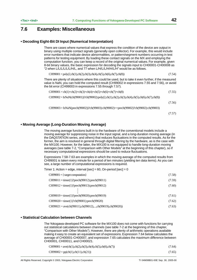
42
All Rights Reserved. Copyright © 2003, Yokogawa Electric Corporation
<Toc> <Ind>
TI 04M08B01-00E
7. Computing Functions of Yokogawa-Developed PC Software
Sep. 30, 2005-00
7.6 Examples: Miscellaneous
• Decoding Eight-Bit DI Input (Numerical Interpretation)
There are cases where numerical values that express the condition of the device are output inbinary using multiple contact signals (generally open collector). For example, this would includeerror numbers that indicate device abnormalities, or pattern/segment numbers occurring in testpatterns for testing equipment. By loading these contact signals on the MX and employing thecomputation function, you can keep a record of the original numerical values. For example, given8-bit binary values, the basic expression for decoding the signals input to CH00001-CH00008 as“2 when L/L/L/L/L/L/H/L, and 77 when L/H/L/L/H/H/L/H” would be as follows.
CH99001 = poly(2,ch(1),ch(2),ch(3),ch(4),ch(5),ch(6),ch(7),ch(8)) (7.54)
There are plenty of situations where this could be used, but to take it even further, if the measuredvalue is NaN, you can hold the computed result (CH99002 in expressions 7.55 and 7.56), or avoidthe bit error (CH99003 in expressions 7.55 through 7.57).
CH99001 = ch(1)+ch(2)+ch(3)+ch(4)+ch(5)+ch(6)+ch(7)+ch(8) (7.55)
CH99002 = IsNaN(ch(99001))?ch(99002):poly(2,ch(1),ch(2),ch(3),ch(4),ch(5),ch(6),ch(7),ch(8))
(7.56)
CH99003 = IsNaN(prech(99002))?ch(99003):ch(99002)==prech(99002)?ch(99002):ch(99003)
(7.57)
• Moving Average (Long-Duration Moving Average)
The moving average functions built in to the hardware of the conventional models include amoving average for suppressing noise in the input signal, and a long-duration moving average (inthe DAQSTATION series, and others) that reduces fluctuations in the computed results. As for theformer, the aim is resolved in general through digital filtering by the hardware, as is the case withthe MX100. However, for the latter, the MX100 is not equipped to handle long-duration movingaverages (see table 7-2, “Comparison with Other Models” at the beginning of this chapter), so ifnecessary computational expressions should be used to reduce fluctuations.
Expressions 7.58-7.63 are examples in which the moving average of the computed results fromCH99001 is taken every minute for a period of ten minutes (yielding ten data items). As you cansee, a large number of computational expressions is required.
Timer 1: Action = edge, interval [sec] = 60, On-period [sec] = 0
CH99001 = { target computation} (7.58)
CH99011 = timer(1)?prech(99012):prech(99011) (7.59)
CH99012 = timer(1)?prech(99013):prech(99012) (7.60)
CH99019 = timer(1)?prech(99020):prech(99019) (7.61)
CH99020 = timer(1)?ch(99001):prech(99020) (7.62)
CH99021 = ave(ch(99011),ch(99012),...,ch(99019),ch(99020)) (7.63)
• Statistical Calculation between Channels
The Yokogawa-developed PC software for the MX100 does not come with functions for carryingout statistical calculations between channels (see table 7-2 at the beginning of this chapter,“Comparison with Other Models”). However, there are plenty of arithmetic operations availablemaking it easy to create an equivalent set of expressions. Expression 7.64 below calculates theaverage of CH00001-CH00007, and expression 7.65 calculates the maximum difference betweenCH00001, CH00011, and CH00021.
CH99001 = ave(ch(1),ch(2),ch(3),ch(4),ch(5),ch(6),ch(7)) (7.64)
CH99002 = pp(ch(1),ch(11),ch(21)) (7.65)

All Rights Reserved. Copyright © 2003, Yokogawa Electric Corporation TI 04M08B01-00E
43<Toc> <Ind> 7. Computing Functions of Yokogawa-Developed PC Software
• OR Alarm on Arbitrary Channels
There are times when you want to output alarms using one DO when one of several alarmconditions becomes true. On MXLOGGER, you can specify a range of reference channels for thealarm as a digital output condition, but you are otherwise limited in the selection of channels: forexample, you cannot specify multiple non-consecutive channels. And on the MX StandardSoftware, you cannot even select a range at all. In these cases, you can implement OR alarmswith expressions. In this example, we have contact output on CH00031 turn ON when either thecondition for alarm level 1 on CH00001 or alarm level 2 on CH00011 is reached.
CH00031 : Action = alarm, reference channel = CH99001, level 1, hold = non-hold
CH99001 : alarm 1 type = High, alarm 1 setting = 0.5, alarm 1 hysteresis = 0
CH99001 = alarm(1,1)||alarm(11,2) (7.66)
However, since this is a result computed by the PC software, the operation occurs more slowlycompared to hardware based alarms, and you must be aware that operations can fail duringcommunication abnormalities. Also, if you attempt to hold output using this method, the fact thattroubles such as failure in detection of newly occurring alarms can occur means that you need amore accurate technique (not provided herein).
7.7 Notes When Writing Computational Expressions andTechniques to Avoid Problems (Description)In “Techniques That Take Communication into Account” at the beginning of this chapter, there is abrief explanation of points to consider regarding the communication between the MX100 which isperforming measurement and the PC which is performing computation. Techniques for resolvingrelated issues were also touched on briefly. In this section, detailed examples and explanationsare provided to help you understand these points and techniques in greater depth.
The table below gives an overview of the points that should be noted regarding the writing ofcomputational expressions.
Table 7-3 Points to Note When Writing Computational Expressions
T0703.EPS
Issue
Use the IsNaN() or sum() function
Cause
Determination of operation conditions based on measured values, measured value summing without TLOG function, other
Method
Communication broken, or data not received immediately after monitoring starts
It is possible for the referenced result from the measurement channel to be NaN.
Key Points
Measured data via communications received too late
Comparison with previous value of measurement channel (detection of changes in contact or other signals), other
Load into the computation channel first
1
No.
2
The referenced result from the measurement channel of the prech() function is not necessarily the previous value of the ch() function.
To understand these points better, we will first briefly explain how to incorporate measured valuesinto computational expressions, and the conditions under which referenced results from themeasurement channel can be NaN, and then give specific examples and techniques.
• Incorporating Measured Values and Other Parameters into Computational Expressions
The ch() and prech() functions are available as a means of incorporating measured values intocomputational expressions. However, unlike computational expressions which are executed onthe PC at fixed intervals, measured values are not necessarily obtained at fixed intervals. This isbecause communication takes place between the MX main unit and PC, and the measurementson the MX and computations on the PC are not synchronized. Therefore, you must be aware thatthe time series of the data measured on the MX main unit does not necessarily match the timeseries incorporated into the computational expression by the ch() function. Figure 7-11 and Table7-4 show how the ch() and prech() functions are affected depending on the delay of arrival ofmeasured data.
Sep. 30, 2005-00
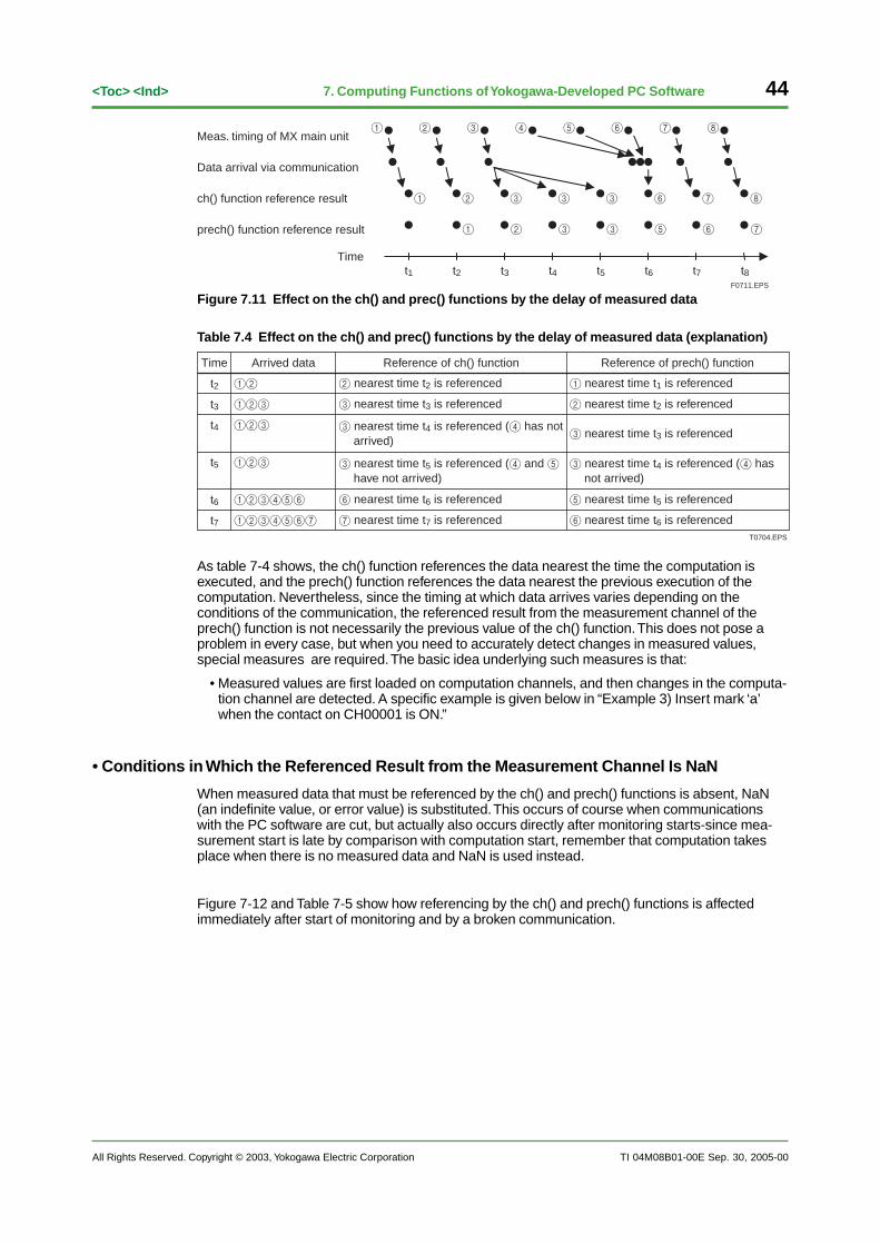
44
All Rights Reserved. Copyright © 2003, Yokogawa Electric Corporation
<Toc> <Ind>
TI 04M08B01-00E
7. Computing Functions of Yokogawa-Developed PC Software
F0711.EPS
t1 t2 t3 t4 t5 t6 t7 t8Time
1 2 3 4 5 6 7 8Meas. timing of MX main unit
Data arrival via communication
ch() function reference result
prech() function reference result
1 2 3 3 3 6 7 8
1 2 3 3 5 6 7
Figure 7.11 Effect on the ch() and prec() functions by the delay of measured data
Table 7.4 Effect on the ch() and prec() functions by the delay of measured data (explanation)
Reference of ch() function
3 nearest time t5 is referenced (4 and 5 have not arrived)
Arrived data
2 nearest time t2 is referenced 1 nearest time t1 is referenced
Reference of prech() function
3 nearest time t4 is referenced (4 has not arrived)
123
123
12
6 nearest time t6 is referenced
123
123456
3 nearest time t3 is referenced
6 nearest time t6 is referenced
5 nearest time t5 is referenced
7 nearest time t7 is referenced
Time
2 nearest time t2 is referenced
3 nearest time t3 is referenced
3 nearest time t4 is referenced (4 has not arrived)
1234567
t4
t3
t7
t2
t6
t5
T0704.EPS
As table 7-4 shows, the ch() function references the data nearest the time the computation isexecuted, and the prech() function references the data nearest the previous execution of thecomputation. Nevertheless, since the timing at which data arrives varies depending on theconditions of the communication, the referenced result from the measurement channel of theprech() function is not necessarily the previous value of the ch() function. This does not pose aproblem in every case, but when you need to accurately detect changes in measured values,special measures are required. The basic idea underlying such measures is that:
• Measured values are first loaded on computation channels, and then changes in the computa-tion channel are detected. A specific example is given below in “Example 3) Insert mark ‘a’when the contact on CH00001 is ON.”
• Conditions in Which the Referenced Result from the Measurement Channel Is NaN
When measured data that must be referenced by the ch() and prech() functions is absent, NaN(an indefinite value, or error value) is substituted. This occurs of course when communicationswith the PC software are cut, but actually also occurs directly after monitoring starts-since mea-surement start is late by comparison with computation start, remember that computation takesplace when there is no measured data and NaN is used instead.
Figure 7-12 and Table 7-5 show how referencing by the ch() and prech() functions is affectedimmediately after start of monitoring and by a broken communication.
Sep. 30, 2005-00
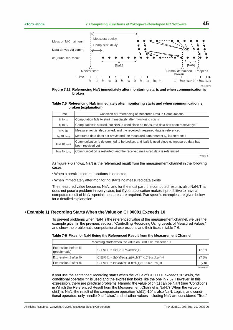
All Rights Reserved. Copyright © 2003, Yokogawa Electric Corporation TI 04M08B01-00E
45<Toc> <Ind> 7. Computing Functions of Yokogawa-Developed PC Software
F0712.EPS
t0
[NaN][NaN]
t1 t2 t3 t4 t5 t6 t7 t8 t9 t10 t11 tN tN+1 tN+2 tN+3 tN+4 tN+5
Comp. start delay
Meas. start delay
Comm. deteminedbroken
Reopens
Time
Monitor start
Meas on MX main unit
Data arrives via comm.
ch() func. rec. result
Figure 7.12 Referencing NaN immediately after monitoring starts and when communication is broken
Table 7.5 Referencing NaN immediately after monitoring starts and when communication is broken (explanation)
Computation fails to start immediately after monitoring starts
Condition of Referencing of Measured Data in Computations
Communication is restarted, and the received measured data is referenced
Communication is determined to be broken, and NaN is used since no measured data has been received yet
Time
Computation is started, but NaN is used since no measured data has been received yet
Measurement is also started, and the received measured data is referenced
Measured data does not arrive, and the measured data nearest t10 is referenced
t9 to t10
t2 to t8
tN+4 to tN+5
t0 to t1
tN+2 to tN+3
t11 to tN+1
T0705.EPS
As figure 7-5 shows, NaN is the referenced result from the measurement channel in the followingcases.
• When a break in communications is detected
• When immediately after monitoring starts no measured data exists
The measured value becomes NaN, and for the most part, the computed result is also NaN. Thisdoes not pose a problem in every case, but if your application makes it prohibitive to have acomputed result of NaN, special measures are required. Two specific examples are given belowfor a detailed explanation.
• Example 1) Recording Starts When the Value on CH00001 Exceeds 10
To prevent problems when NaN is the referenced value of the measurement channel, we use theexample given in the previous section, “Controlling Recording Using Levels of Measured Values,”and show the problematic computational expressions and their fixes in table 7-6.
Table 7-6 Fixes for NaN Being the Referenced Result from the Measurement Channel
CH99001 = ch(1)>10?StartRec():0
Recording starts when the value on CH00001 exceeds 10
CH99001 = (IsNaN(ch(1))?0:ch(1))>10?StartRec():0
CH99001 = IsNaN(ch(1))?0:ch(1)>10?StartRec():0
(7.67)
(7.68)
(7.8)Expression 2 after fix
Expression 1 after fix
Expression before fix (problematic)
T0706.EPS
If you use the sentence “Recording starts when the value of CH00001 exceeds 10” as-is, theconditional operator “?” is used and the expression looks like the one in 7.67. However, in thisexpression, there are practical problems. Namely, the value of ch(1) can be NaN (see “Conditionsin Which the Referenced Result from the Measurement Channel is NaN.”) When the value ofch(1) is NaN, the result of the comparison operation “ch(1)>10” is also NaN. Logical and condi-tional operators only handle 0 as “false,” and all other values including NaN are considered “True.”
Sep. 30, 2005-00
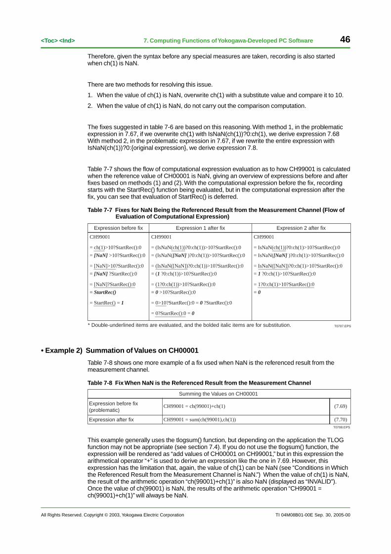
46
All Rights Reserved. Copyright © 2003, Yokogawa Electric Corporation
<Toc> <Ind>
TI 04M08B01-00E
7. Computing Functions of Yokogawa-Developed PC Software
Therefore, given the syntax before any special measures are taken, recording is also startedwhen ch(1) is NaN.
There are two methods for resolving this issue.
1. When the value of ch(1) is NaN, overwrite ch(1) with a substitute value and compare it to 10.
2. When the value of ch(1) is NaN, do not carry out the comparison computation.
The fixes suggested in table 7-6 are based on this reasoning. With method 1, in the problematicexpression in 7.67, if we overwrite ch(1) with IsNaN(ch(1))?0:ch(1), we derive expression 7.68With method 2, in the problematic expression in 7.67, if we rewrite the entire expression withIsNaN(ch(1))?0:{original expression}, we derive expression 7.8.
Table 7-7 shows the flow of computational expression evaluation as to how CH99001 is calculatedwhen the reference value of CH00001 is NaN, giving an overview of expressions before and afterfixes based on methods (1) and (2). With the computational expression before the fix, recordingstarts with the StartRec() function being evaluated, but in the computational expression after thefix, you can see that evaluation of StartRec() is deferred.
Table 7-7 Fixes for NaN Being the Referenced Result from the Measurement Channel (Flow ofEvaluation of Computational Expression)
CH99001
= IsNaN(ch(1))?0:ch(1)>10?StartRec():0
= IsNaN([NaN] )?0:ch(1)>10?StartRec():0
= IsNaN([NaN])?0:ch(1)>10?StartRec():0
= 1 ?0:ch(1)>10?StartRec():0
= 1?0:ch(1)>10?StartRec():0
= 0
CH99001
= (IsNaN(ch(1))?0:ch(1))>10?StartRec():0
= (IsNaN([NaN] )?0:ch(1))>10?StartRec():0
= (IsNaN([NaN])?0:ch(1))>10?StartRec():0
= (1 ?0:ch(1))>10?StartRec():0
= (1?0:ch(1))>10?StartRec():0
= 0 >10?StartRec():0
= 0>10?StartRec():0 = 0 ?StartRec():0
= 0?StartRec():0 = 0
CH99001
= ch(1)>10?StartRec():0
= [NaN] >10?StartRec():0
= [NaN]>10?StartRec():0
= [NaN] ?StartRec():0
= [NaN]?StartRec():0
= StartRec()
= StartRec() = 1
Expression before fix Expression 1 after fix Expression 2 after fix
* Double-underlined items are evaluated, and the bolded italic items are for substitution. T0707.EPS
• Example 2) Summation of Values on CH00001
Table 7-8 shows one more example of a fix used when NaN is the referenced result from themeasurement channel.
Table 7-8 Fix When NaN is the Referenced Result from the Measurement Channel
CH99001 = ch(99001)+ch(1)
Summing the Values on CH00001
CH99001 = sum(ch(99001),ch(1))
(7.69)
(7.70)Expression after fix
Expression before fix (problematic)
T0708.EPS
This example generally uses the tlogsum() function, but depending on the application the TLOGfunction may not be appropriate (see section 7.4). If you do not use the tlogsum() function, theexpression will be rendered as “add values of CH00001 on CH99001,” but in this expression thearithmetical operator “+” is used to derive an expression like the one in 7.69. However, thisexpression has the limitation that, again, the value of ch(1) can be NaN (see “Conditions in Whichthe Referenced Result from the Measurement Channel is NaN.”) When the value of ch(1) is NaN,the result of the arithmetic operation “ch(99001)+ch(1)” is also NaN (displayed as “INVALID”).Once the value of ch(99001) is NaN, the results of the arithmetic operation “CH99001 =ch(99001)+ch(1)” will always be NaN.
Sep. 30, 2005-00
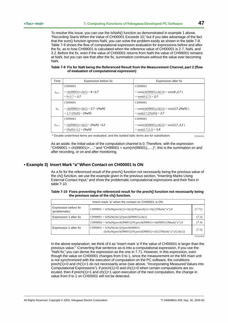
All Rights Reserved. Copyright © 2003, Yokogawa Electric Corporation TI 04M08B01-00E
47<Toc> <Ind> 7. Computing Functions of Yokogawa-Developed PC Software
To resolve this issue, you can use the IsNaN() function as demonstrated in example 1 above,“Recording Starts When the Value of CH00001 Exceeds 10,” but if you take advantage of the factthat the sum() function ignores NaN, you can solve the problem easily as shown in the table 7-8.Table 7-9 shows the flow of computational expression evaluation for expressions before and afterthe fix, as to how CH99001 is calculated when the reference value of CH00001 is 2.7, NaN, and3.2. Before the fix, even if the value of CH00001 returns from NaN the value of CH99001 remainsat NaN, but you can see that after the fix, summation continues without the value ever becomingNaN.
Table 7-9 Fix for NaN being the Referenced Result from the Measurement Channel, part 2 (flowof evaluation of computational expression)
CH99001
= sum(ch(99001),ch(1)) = sum(0 ,2.7 )
= sum(0,2.7) = 2.7
CH99001
= ch(99001)+ch(1) = 0 +2.7
= 0+2.7 = 2.7tN-1
CH99001
= sum(ch(99001),ch(1)) = sum(2.7 ,[NaN] )
= sum(2.7,[NaN]) = 2.7
CH99001
= ch(99001)+ch(1) = 2.7 +[NaN]
= 2.7+[NaN] = [NaN]
tN
CH99001
= sum(ch(99001),ch(1)) = sum(2.7 ,3.2 )
= sum(2.7,3.2) = 5.9
CH99001
= ch(99001)+ch(1) = [NaN] +3.2
= [NaN]+3.2 = [NaN]
tN+1
Time Expression before fix Expression after fix
T0709.EPS* Double-underlined items are evaluated, and the bolded italic items are for substitution.
As an aside, the initial value of the computation channel is 0. Therefore, with the expression“CH99001 = ch(99001)+.....” and “CH99001 = sum(ch(99001),.....)”, this is the summation on andafter recording, or on and after monitoring.
• Example 3) Insert Mark “a” When Contact on CH00001 Is ON
As a fix for the referenced result of the prech() function not necessarily being the previous value ofthe ch() function, we use the example given in the previous section, “Inserting Marks UsingExternal Contact Input,” and show the problematic computational expressions and their fixes intable 7-10.
Table 7-10 Fixes preventing the referenced result for the prech() function not necessarily being the previous value of the ch() function.
CH99001 = IsNaN(prech(1)+ch(1))?0:prech(1)<ch(1)?Mark(“a”):0
Insert mark “a” when the contact on CH00001 is ON
CH99001 = IsNaN(ch(1))?prech(99001):ch(1)
(7.71)
(7.3)Expression 1 after fix
Expression before fix (problematic)
CH99002 = IsNaN(prech(99001))?0:prech(99001)<ch(99001)?Mark("a"):0
CH99001 = IsNaN(ch(1))?prech(99001) :(IsNaN(prech(99001))?0:prech(99001)<ch(1)?Mark(“a”):0,ch(1))
(7.4)
(7.5)Expression 2 after fix
T0710.EPS
In the above explanation, we think of it as “insert mark ‘a’ if the value of CH00001 is larger than theprevious value.” Converting that sentence as-is into a computational expression, if you use the“NaN fix,” you can derive the expression as the one in 7.71. However, in this expression, eventhough the value on CH00001 changes from 0 to 1, since the measurement on the MX main unitis not synchronized with the execution of computation on the PC software, the conditionsprech(1)=0 and ch(1)=1 do not necessarily arise (see above, “Incorporating Measured Values intoComputational Expressions”). If prech(1)=0 and ch(1)=0 when certain computations are ex-ecuted, then if prech(1)=1 and ch(1)=1 upon execution of the next computation, the change invalue from 0 to 1 on CH00001 will not be detected.
Sep. 30, 2005-00
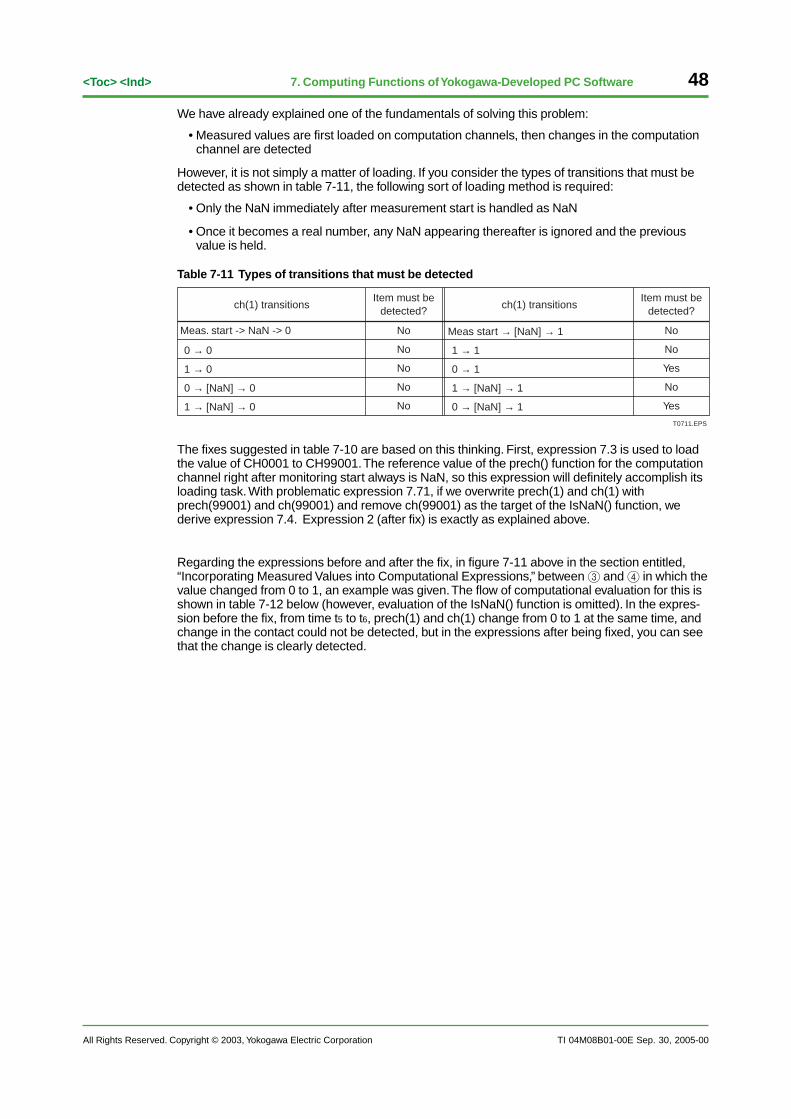
48
All Rights Reserved. Copyright © 2003, Yokogawa Electric Corporation
<Toc> <Ind>
TI 04M08B01-00E
7. Computing Functions of Yokogawa-Developed PC Software
We have already explained one of the fundamentals of solving this problem:
• Measured values are first loaded on computation channels, then changes in the computationchannel are detected
However, it is not simply a matter of loading. If you consider the types of transitions that must bedetected as shown in table 7-11, the following sort of loading method is required:
• Only the NaN immediately after measurement start is handled as NaN
• Once it becomes a real number, any NaN appearing thereafter is ignored and the previousvalue is held.
Table 7-11 Types of transitions that must be detected
1 → 1
0 → 1
1 → [NaN] → 1
No
Item must be detected?
Meas start → [NaN] → 1
ch(1) transitions
No
No
No
No
0 → [NaN] → 1 Yes
Yes
No
No
No
Item must be detected?
ch(1) transitions
Meas. start -> NaN -> 0
1 → 0
0 → [NaN] → 0
1 → [NaN] → 0
0 → 0
T0711.EPS
The fixes suggested in table 7-10 are based on this thinking. First, expression 7.3 is used to loadthe value of CH0001 to CH99001. The reference value of the prech() function for the computationchannel right after monitoring start always is NaN, so this expression will definitely accomplish itsloading task. With problematic expression 7.71, if we overwrite prech(1) and ch(1) withprech(99001) and ch(99001) and remove ch(99001) as the target of the IsNaN() function, wederive expression 7.4. Expression 2 (after fix) is exactly as explained above.
Regarding the expressions before and after the fix, in figure 7-11 above in the section entitled,“Incorporating Measured Values into Computational Expressions,” between 3 and 4 in which thevalue changed from 0 to 1, an example was given. The flow of computational evaluation for this isshown in table 7-12 below (however, evaluation of the IsNaN() function is omitted). In the expres-sion before the fix, from time t5 to t6, prech(1) and ch(1) change from 0 to 1 at the same time, andchange in the contact could not be detected, but in the expressions after being fixed, you can seethat the change is clearly detected.
Sep. 30, 2005-00
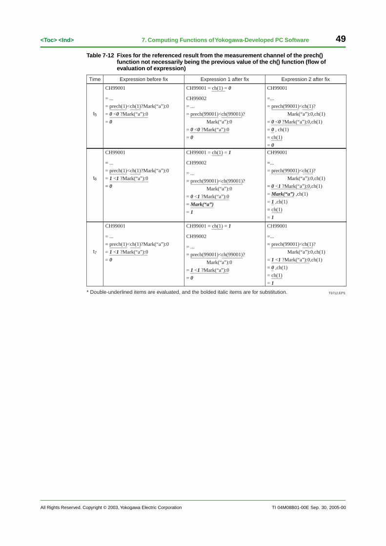
All Rights Reserved. Copyright © 2003, Yokogawa Electric Corporation TI 04M08B01-00E
49<Toc> <Ind> 7. Computing Functions of Yokogawa-Developed PC Software
Sep. 30, 2005-00
Table 7-12 Fixes for the referenced result from the measurement channel of the prech()function not necessarily being the previous value of the ch() function (flow ofevaluation of expression)
CH99001
=...
= prech(99001)<ch(1)?
Mark(“a”):0,ch(1)
= 0 <0 ?Mark(“a”):0,ch(1)
= 0 , ch(1)
= ch(1)
= 0
CH99001 = ch(1) = 0
CH99002
= ...
= prech(99001)<ch(99001)?
Mark(“a”):0
= 0 <0 ?Mark(“a”):0
= 0
CH99001
= ...
= prech(1)<ch(1)?Mark(“a”):0
= 0 <0 ?Mark(“a”):0
= 0
CH99001
=...
= prech(99001)<ch(1)?
Mark(“a”):0,ch(1)
= 0 <1 ?Mark(“a”):0,ch(1)
= Mark(“a”) ,ch(1)
= 1 ,ch(1)
= ch(1)
= 1
CH99001 = ch(1) = 1
CH99002
= ...
= prech(99001)<ch(99001)?
Mark(“a”):0
= 0 <1 ?Mark(“a”):0
= Mark(“a”)
= 1
CH99001
= ...
= prech(1)<ch(1)?Mark(“a”):0
= 1 <1 ?Mark(“a”):0
= 0
CH99001
=...
= prech(99001)<ch(1)?
Mark(“a”):0,ch(1)
= 1 <1 ?Mark(“a”):0,ch(1)
= 0 ,ch(1)
= ch(1)
= 1
CH99001 = ch(1) = 1
CH99002
= ...
= prech(99001)<ch(99001)?
Mark(“a”):0
= 1 <1 ?Mark(“a”):0
= 0
CH99001
= ...
= prech(1)<ch(1)?Mark(“a”):0
= 1 <1 ?Mark(“a”):0
= 0
Expression before fix Expression 1 after fix Expression 2 after fix
T0712.EPS
Time
t5
t6
t7
* Double-underlined items are evaluated, and the bolded italic items are for substitution.
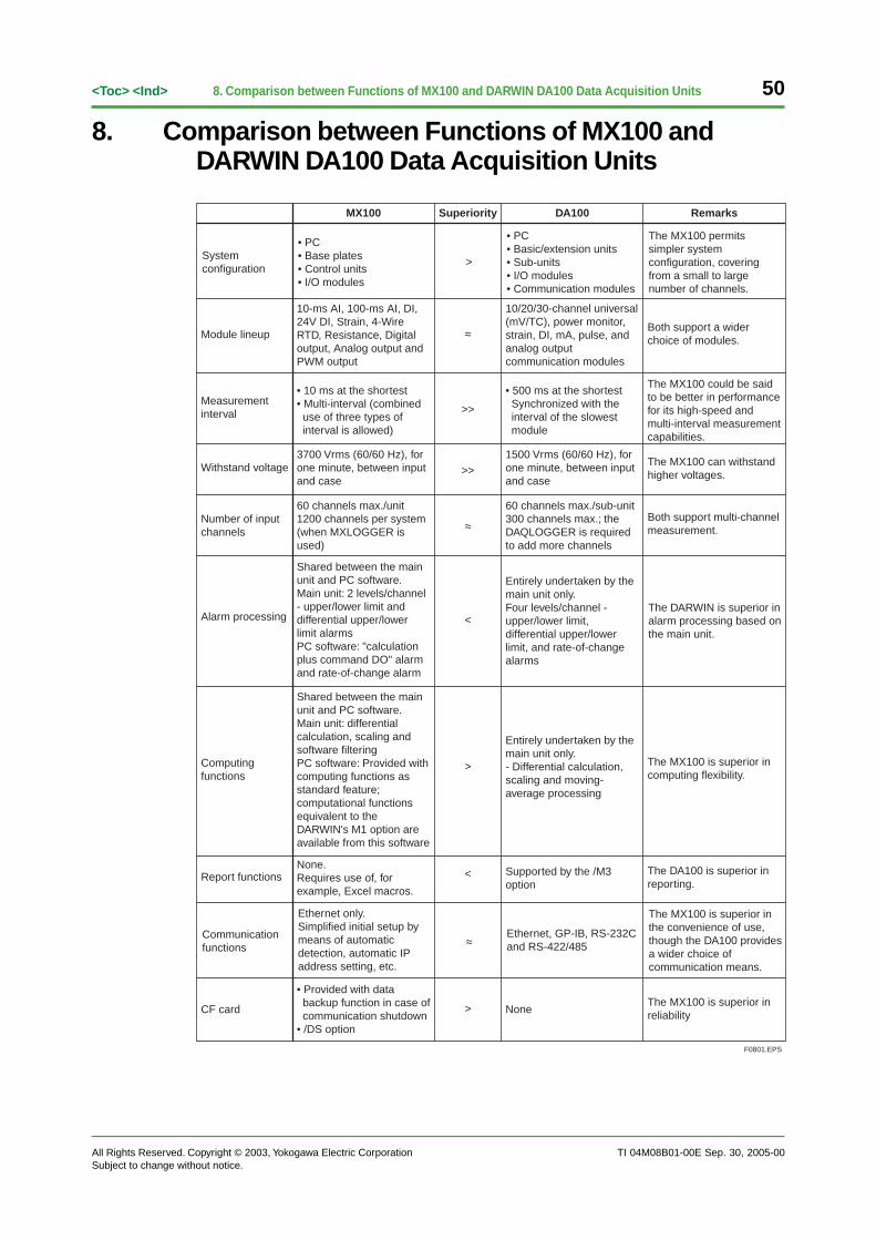
50
All Rights Reserved. Copyright © 2003, Yokogawa Electric CorporationSubject to change without notice.
<Toc> <Ind>
TI 04M08B01-00E
8. Comparison between Functions of MX100 and DARWIN DA100 Data Acquisition Units
Sep. 30, 2005-00
8. Comparison between Functions of MX100 andDARWIN DA100 Data Acquisition Units
System configuration
MX100 Superiority DA100 Remarks
Module lineup
Measurement interval
Withstand voltage
Number of input channels
Alarm processing
Computing functions
Report functions
Communication functions
CF card
>
≈
>>
>>
≈
<
>
<
≈
>
• PC• Base plates• Control units• I/O modules
• 10 ms at the shortest• Multi-interval (combined use of three types of interval is allowed)
Ethernet only.Simplified initial setup by means of automatic detection, automatic IP address setting, etc.
60 channels max./unit1200 channels per system (when MXLOGGER is used)
Shared between the main unit and PC software.Main unit: 2 levels/channel - upper/lower limit and differential upper/lower limit alarmsPC software: "calculation plus command DO" alarm and rate-of-change alarm
3700 Vrms (60/60 Hz), for one minute, between input and case
None.Requires use of, for example, Excel macros.
• Provided with data backup function in case of communication shutdown
• /DS option
10-ms AI, 100-ms AI, DI,24V DI, Strain, 4-Wire RTD, Resistance, Digital output, Analog output and PWM output
Shared between the main unit and PC software.Main unit: differential calculation, scaling and software filteringPC software: Provided with computing functions as standard feature; computational functions equivalent to the DARWIN's M1 option are available from this software
• PC• Basic/extension units• Sub-units• I/O modules• Communication modules
• 500 ms at the shortestSynchronized with the interval of the slowest module
Ethernet, GP-IB, RS-232C and RS-422/485
60 channels max./sub-unit300 channels max.; the DAQLOGGER is required to add more channels
Entirely undertaken by the main unit only.Four levels/channel - upper/lower limit, differential upper/lower limit, and rate-of-change alarms
1500 Vrms (60/60 Hz), for one minute, between input and case
Supported by the /M3 option
None
10/20/30-channel universal (mV/TC), power monitor, strain, DI, mA, pulse, and analog output communication modules
Entirely undertaken by the main unit only.- Differential calculation, scaling and moving-average processing
The MX100 permits simpler system configuration, covering from a small to large number of channels.
The MX100 could be said to be better in performance for its high-speed and multi-interval measurement capabilities.
The MX100 is superior in the convenience of use, though the DA100 provides a wider choice of communication means.
Both support multi-channel measurement.
The MX100 can withstand higher voltages.
The DA100 is superior in reporting.
The MX100 is superior in reliability
Both support a wider choice of modules.
The MX100 is superior in computing flexibility.
The DARWIN is superior in alarm processing based on the main unit.
F0801.EPS


![[Manuale - ITA] Warhammer 40000 to](https://img.pdfslide.us/doc/110x75/54f7d9364a7959303c8b494e/manuale-ita-warhammer-40000-to.jpg)