Embed Size (px)
Citation preview
ii | P a g e
Technical Improvements to the Greenhouse Gas (GHG)
Inventory for California Forests and Other Lands FINAL REPORT
Prepared for the California Air Resources Board and the California Environmental Protection Agency: Agreement #14-757
Principal Investigator, David Saah
Submitted By:
May, 2016
i | P a g e
Recommended Report Citation: Saah D., J. Battles, J. Gunn, T. Buchholz, D. Schmidt, G. Roller, and S. Romsos. 2015. Technical improvements to the greenhouse gas (GHG) inventory for California forests and other lands. Submitted to: California Air Resources Board, Agreement #14-757. 55 pages.
DISCLAIMER The statements and conclusions in this report are those of the authors from the Spatial Informatics
Group, and not necessarily those of the California Air Resources Board. The mention of
commercial products, their source, or their use in connection with material reported herein is not
to be construed as actual or implied endorsement of such products.
ACKNOWLEDGEMENTS This Report was submitted in fulfillment of ARB Agreement #14-757, Technical Improvements to
the Greenhouse Gas (GHG) Inventory for California Forests and Other Lands by Spatial
Informatics Group, LLC under the partial sponsorship of the California Air Resources Board. We
thank Scott Stephens for providing access to the field data from the Blodgett site of the Fire and
Fire Surrogates Study. We also thank Malcolm North for allowing us to use the Sagehen field data
and UC Berkeley for the use of the Sierra Nevada Adaptive Management Project (SNAMP) data.
Bill Van Doren from Spatial Informatics Group assisted with analysis of the FIA data. Klaus Scott
and John Dingman from the California Air Resources Board made significant technical and
intellectual contributions throughout this project. Work was completed as of May, 2016
ii | P a g e
TABLE OF CONTENTS Disclaimer ..................................................................................................................................................... i
Acknowledgements ..................................................................................................................................... i
List of Figures ............................................................................................................................................ iv
List of Tables .............................................................................................................................................. iv
Executive Summary .................................................................................................................................. vi
Introduction .................................................................................................................................................. 1
Project Background ................................................................................................................................ 1
Physical and Operational Boundaries (Scope) .................................................................................. 4
Objectives ................................................................................................................................................ 5
Report Organization ............................................................................................................................... 6
Methods and Results ................................................................................................................................. 7
Step 1: Review of 2010 LANDFIRE Vegetation Type Category Changes .................................... 7
Step 2: Integration of LANDFIRE EVT, EVC and EVH Data Layers ............................................ 12
Step 3: Crosswalk IPCC Land Categories with 2010 Carbon Accounting Layer Categories... 12
Step 4: Literature and Data Review and Summary of Biomass and Carbon Associated
Agriculture and Urban Landscapes. .................................................................................................. 13
Agriculture and Urban Vegetation Types ...................................................................................... 13
Step 5: Evaluation of Dead Carbon Pools ........................................................................................ 23
Field Plot Data Analysis .................................................................................................................. 24
FIA Data Comparison ...................................................................................................................... 26
Step 6: Identify Carbon Considerations of Forest Management and Harvested Wood Products
................................................................................................................................................................ 28
Harvest Operations in California .................................................................................................... 28
Wood Products Carbon Assessment ............................................................................................ 29
Validation ........................................................................................................................................... 30
Landscape Harvest Impact 2001-2010 ......................................................................................... 30
Reported Harvest Intensities .......................................................................................................... 32
Reported Harvest Volumes ............................................................................................................. 32
Step 7: Accounting for Undetected Biomass Growth ..................................................................... 32
Step 8: Updated Lookup Tables and Geographic Information System Data (the Updated GHG
Inventory Tool) ...................................................................................................................................... 34
Step 9: Conduct Carbon Stock Change Evaluation ........................................................................ 36
iii | P a g e
Conclusions, Recommendations and Next Steps ............................................................................... 40
References ................................................................................................................................................ 41
Appendices ................................................................................................................................................ 45
iv | P a g e
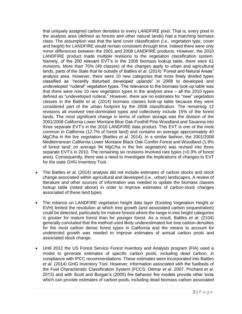
LIST OF FIGURES Figure 1. Steps used to update Battle et al. (2014) GHG Inventory Tool. ......................................... 7
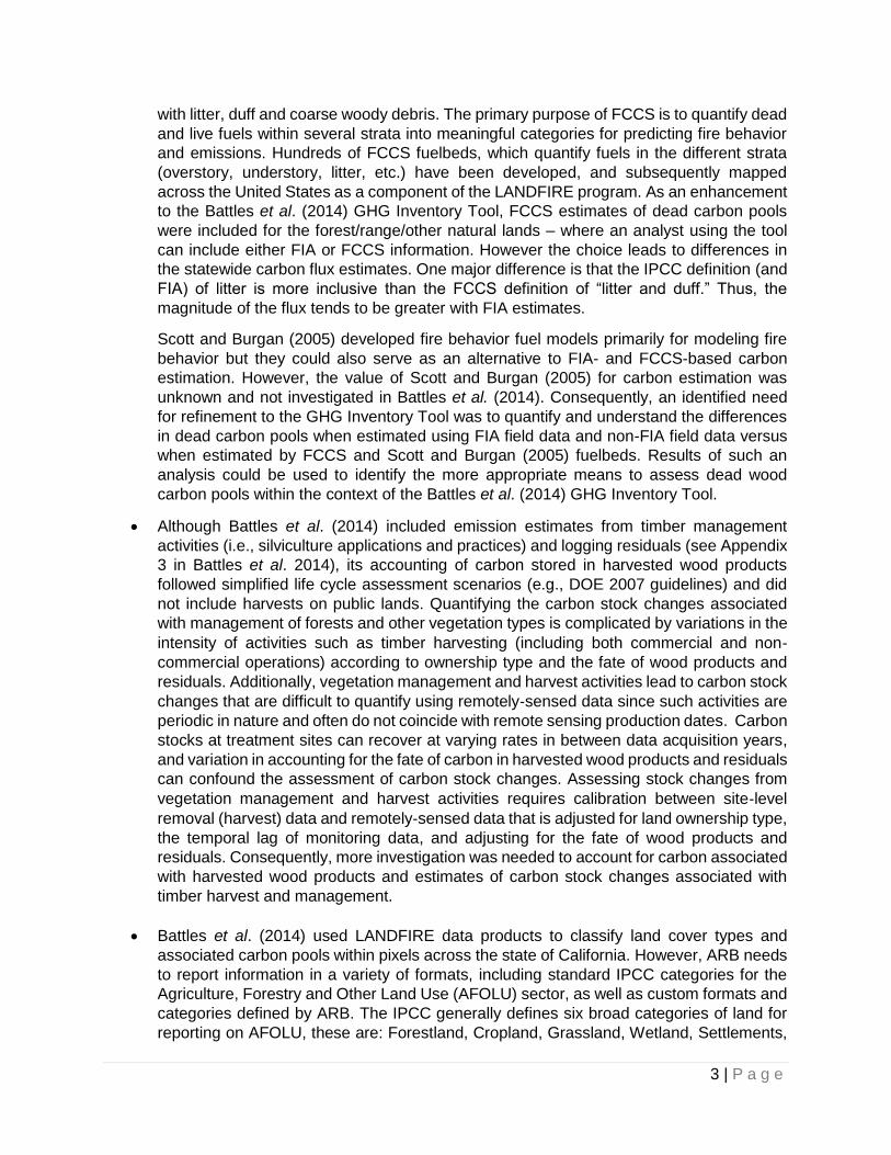
Figure 2. Predicted variation in ALB as a function of cover and height class. A) Results for the
forest/woodland submodel; B) Results for the savanna submodel. ................................................. 11
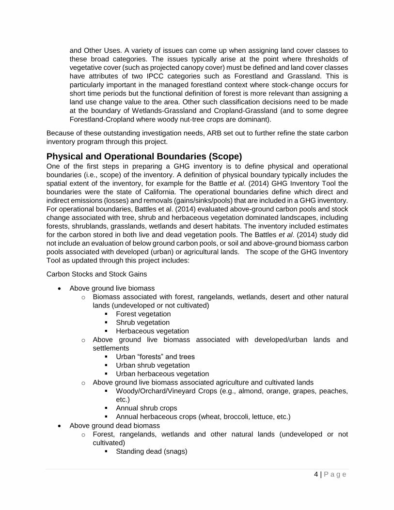
Figure 3. Differences in predicted ALB for each submodel compared to inclusive model. A)
Results for the forest/woodland submodel; B) Results for the savanna submodel. ...................... 12
Figure 4. Distribution of changes in aboveground live biomass for 966 repeat measures FIA plots
that remained forest from 2001-2002 to their re-measurement dates in 2011 and 2002. ............ 33
Figure 5. Closer examination of the distribution of changes in aboveground live biomass growth
for 966 re-measured plots in the FIA data. This histogram clearly shows the many more small
gains in biomass compared to small losses. ........................................................................................ 33
LIST OF TABLES Table 1. Vegetation classification levels, classification criteria and examples of the levels of the
National Vegetation Classification Standard hierarchy for natural vegetation. ................................. 8
Table 2. Number of existing vegetation types (EVT’s) by major landuse type in California from
three LANDFIRE data iterations (2001, 2008 and 2011). .................................................................... 9
Table 3. Comparison of relative variable importance (rVIP) for determination of floristic
classification versus determination of carbon density for 277 blue oak woodland FIA plots. ...... 10
Table 4. Source of biomass and carbon values assigned to different LANDFIRE existing
vegetation types (EVT) and IPCC AFOLU categories. Values were either sources from existing
literature or databases, calculated using accepted methods or drawn from IPCC Tier 1 default
values. ........................................................................................................................................................ 14
Table 5. Summary of evaluation approach used to calculate aboveground biomass and carbon
estimates. .................................................................................................................................................. 15
Table 6. Estimated carbon content of 2014 peak yields of common agricultural commodities of
California (National Agricultural Statistics Service 2015). .................................................................. 16
Table 7. Carbon density estimates of different crops using whole tree/plant biomass and typical
planting density. ........................................................................................................................................ 17
Table 8. Dry matter content factor and harvest Index for common crop types (Summarized from
Table 3-5 in Eve et al. 2014). ................................................................................................................. 19
Table 9. Carbon estimates of row and close grown crops by agricultural district. ......................... 20
Table 10. Carbon estimates of crops using harvest residue biomass estimates (Mitchell et al.
1999) and yield estimates (National Agricultural Statistics Service 2015). ..................................... 21
Table 11. Urban forest carbon estimates by county in California (from Bjorkman et al. 2015). .. 22
Table 12. Default IPCC Values for carbon for cultivated and managed land, bare areas, and water,
snow, ice and artificial surfaces. IPCC default values of 5 were used for cultivated and managed
land and 1 for bare/fallow/idle areas. .................................................................................................... 23
Table 13. Percent difference in LANDFIRE FCCS dead carbon pool relative to field plot data (S =
sounds, R = rotten). ................................................................................................................................. 25
Table 14. Percent difference of LANDFIRE FBFM40 dead carbon pool relative to field data. .... 26
Table 15. Percent difference across all ecological subregions between FCCS and FIA, and FBFM
and FIA ...................................................................................................................................................... 26
Table 16. Harvest-related disturbance types in LANDFIRE Disturbance 1999-2012 dataset
(Source: LANDFIRE 2015). .................................................................................................................... 29
v | P a g e
Table 17. Landscape carbon loss and merchantable volumes on private (Stewart and Nakamura
2012) and public (Saah et al. 2012) land. ............................................................................................ 29
Table 18. Harvested merchantable volumes in million board feet of timber (mmbf) in California
2001-2010 (BOE 2015). .......................................................................................................................... 31
Table 19. Aboveground live carbon loss by harvest type in Mg C/ha 2001-2010. ......................... 31
Table 20. Total net C emissions in Mg for 2001-2010 including carbon stored in wood products
for >100 years. .......................................................................................................................................... 32
Table 21. Merchantable volumes in mmbf and % of total harvested 6/2001 to 6/2010 based on
LANDFIRE data. ....................................................................................................................................... 32
Table 22. Preliminary estimates of total above ground live and dead carbon (not including soil
carbon) in 2001 and 2010 and associated net carbon change by IPCC land category within
California (estimated in MMTC). ............................................................................................................ 37
Table 23. Estimated net changes in above ground live and dead biomass associated carbon
(MMTC) for land conversions occurring in California from 2001 to 2010 by IPCC categories and
subcategories............................................................................................................................................ 38
vi | P a g e
EXECUTIVE SUMMARY In an effort to help reduce changes in climate, the State of California in 2006 enacted the Global
Warming Solutions Act. The Act requires the California Air Resources Board (ARB) to set
statewide GHG emission limits, to develop regulations to reduce emissions, and to regularly
inventory GHG emissions to and removals from the atmosphere. As part of this inventory, the
ARB must account for GHG exchanges in forest and rangeland ecosystems. Under a previous
agreement with ARB (Agreement #10-778), Battles et al. (2014) used Landscape Fire and
Resource Management Planning Tools (LANDFIRE) data products to conduct a stock-change
assessment and track carbon dynamics on forest, range, and other lands in California. Through
this effort, Battles et al. (2014) created a GHG Inventory Tool and provided the first spatial
estimates of above-ground vegetation carbon stock changes and associated uncertainties for the
entire state for natural and working lands sector. However, Battles et al. (2014) noted that there
were areas that needed additional investigation to further refine California’s carbon inventory.
Namely,
1. New vegetation classes were introduced in the 2010 LANDFIRE data products and the
effect of these changes on carbon stock change estimates needed to be understood.
2. Above ground carbon estimates associated with urban and agricultural landscapes were
not included in Battles et al. (2014).
3. Investigation was needed to determine the best source of information for estimating above
ground dead biomass carbon pools.
4. Undetected growth in the largest forest vegetation classes in LANDFIRE needed to be
evaluated and incorporated into the GHG Inventory Tool developed by Battles et al.
(2014).
5. The extent and distribution of timber harvest and forest management throughout California
public and private lands needed to be quantified between 2001 and 2010 – especially for
understanding the implications for above ground carbon stock change assessment.
6. Additional refinement was needed to crosswalk LANDFIRE vegetation classes with IPCC
landuse class to improve reporting under both typologies.
Consequently, this project was designed to refine above-ground forest, rangeland, and other
lands carbon estimates and accounting methods for above-ground biomass originally reported by
Battles et al. (2014) for the Air Resources Board’s periodic California inventory of atmospheric
CO2 removal and greenhouse gas emissions (using a GHG Inventory Tool).
The report is organized around nine steps used to refine Battles et al. (2014) GHG Inventory Tool.
In step 1 of the project, we reviewed changes in the 2010 LANDFIRE vegetation types and found
that changes will not significantly affect the carbon stock change estimates.
In step 2, we used GIS procedures to combine LANDFIRE products which served as a core data
layer and lookup table in the updated GHG Inventory tool.
In step 3, we cross-walked corresponding LANDFIRE vegetation types (as combined with
vegetation height and cover) with IPCC AFOLU land categories.
In step 4, we conducted an extensive literature review to construct estimates of above ground
carbon stocks with associated agriculture and urban landscapes. This information was
summarized and ingested into models and geodatabases (in step 8) to refine estimates of carbon
stock changes between 2001 and 2010 for California’s forests and other lands.
vii | P a g e
For step 5, we quantified the differences in dead biomass (and carbon) pools when estimated
using FIA field data and fuel loading plot data from various study sites, versus when estimated
from LANDFIRE’s FCCS and FBFM (Scott and Burgan fire behavior fuel model) mapping
products. We found that the FCCS fuel behavior model most closely matched field plot and FIA
data on dead biomass (and thus carbon) pools.
In step 6, we summarized the distribution and extent of timber management activities that
occurred between 1999 and 2012 and estimated carbon stocks in residues and in wood products.
We integrated new estimates of carbon in harvested wood products into the updated GHG
Inventory Tool.
In step 7, we evaluated FIA data for the period between 2001 and 2010 to account for forest
growth that is undetectable in LANDFIRE data products due to how large tree heights are
classified. From this assessment we estimated that large tree biomass increased by 6% within
the time period of interest. A coefficient was included for the large tree class to account for
undetected growth in the carbon stock change assessment.
In step 8 we used summaries and information developed in steps 1 through 7 to update the GHG
Inventory Tool. The tool includes database lookup tables, GIS raster layers and geodatabases
that are linked together via ArcGIS models. The GHG Inventory Tool was used to complete step
9 – the carbon stock change assessment for 2001, 2008 and 2010.
Using updated information from steps 1 through 7, GHG Inventory Tool in step 8, and using some
initial assumptions (that may be changed as ARB further develops and refines the tool for its
needs), we preliminarily estimated that between 2001 and 2010, the total above ground carbon
stored in the forests, woodlands, shrublands, grasslands, agricultural, developed/urban and other
lands of California decreased from 2,696 million metric tons of carbon (MMTC) in 2001 to 2,551
MMTC in 2010, representing a potential overall loss of about -145 MMTC over the time period of
interest or a loss of approximately -16.1 MMTC yr-1. The greatest estimated loss in carbon pools
occurred in the form of forest conversion to grassland with wetlands remaining relatively
unchanged across 2001 and 2010. These estimates include above ground live biomass
associated with forestlands, croplands, grasslands, wetlands, urban/developed (IPCC
‘settlements’), and other lands. Stock-changes are reported without attribution by processes such
as wildfire or harvest. Stock-changes associated with wildfire and harvest were estimated
independently and are provided for informational purposes only. Forestlands represent the largest
carbon pool within the study area, storing about 11 times more carbon than other land categories
combined. In addition, we preliminarily assessed the carbon stock changes associated with
landuse conversions between 2001 and 2010 and found that the largest reduction in net above
ground live carbon across wildland, agriculture and urban landscapes was the conversion of the
forestland type to the grassland type, and the greatest gain in above ground live carbon was the
conversion of the wetland type to the forest type.
1 | P a g e
INTRODUCTION In an effort to reduce changes in climate, the State of California in 2006 enacted the Global
Warming Solutions Act (Assembly Bill 32). The Act requires the California Air Resources Board
(ARB) to set statewide GHG emission limits, to develop regulations to reduce emissions, and to
regularly inventory GHG emissions to and removals from the atmosphere. As part of this
inventory, the ARB must account for GHG exchanges in forest and rangeland ecosystems.
Vegetation naturally removes GHG’s from the atmosphere, reducing the magnitude of climate
change. Globally, vegetation and soils removed carbon from the atmosphere at a rate (mean ±
90% CI) of 2.5 ± 1.3 PgC y-1 from 2002 to 2011, compared to fossil fuel emissions of 8.3 ± 0.7
PgC y-1 and deforestation emissions of 0.9 ± 0.8 PgC y-1 (Table 6.1 in Ciais et al. 2013 [i.e.,
Chapter 6 - IPCC 2013]). Recent estimates for California’s forest have varied greatly from a net
carbon uptake of 15.7 million MgC y-1 (Zheng et al. 2011) to net carbon loss of -0.4 million MgC
y-1 (USFS 2013).
Project Background Under an agreement with ARB (Agreement #10-778), Battles et al. (2014) used U.S. Department
of Agriculture Forest Service’s and U.S. Department of the Interior’s - Landscape Fire and
Resource Management Planning Tools (LANDFIRE) data products to conduct a stock-change
assessment and track carbon dynamics on forest, range, and other lands in California. Based on
their stock-change analysis, which included carbon pools in forests and other lands, except above
ground biomass associated with urban and agricultural lands, and soil, Battles et al. (2014)
reported that between 2001 and 2008, the total above ground carbon stored in the forests and
rangelands of California decreased from 2,600 million metric tons of carbon (MMTC = 106 MgC)
to 2,500 MMTC. Aboveground live carbon decreased ~2% and total carbon (which include carbon
associated with dead biomass) decreased ~4%, which represented a statistically significant loss
of carbon with an annual rate of approximately -14 MMTC y-1. Battles et al. (2014) concluded in
general terms that 61% of the loss was due to a reduction in the carbon stored per area (i.e.,
carbon density), with the remaining 39% due to a reduction in size of the analysis area (i.e., due
to wildfire-related transitions of shrublands to grasslands or other land conversions).
Through this effort, Battles et al. (2014) created a GHG Inventory Tool and provided the first
spatial estimates of above-ground vegetation carbon stock changes and associated uncertainties
for the entire state. In doing so, Battles et al. (2014) established the beginning of a time series to
track above-ground carbon stocks and stock-change in California natural ecosystems. However,
Battles et al. (2014) noted that there were several areas that needed additional investigation to
further refine California’s above-ground carbon inventory for forests and other lands, namely:
Battles et al. (2014) relied on land cover metrics provided by LANDFIRE to stratify the
state into fine‐grained (30m by 30m) spatial units. These metrics, defined by LANDFIRE
as Existing Vegetation Type (EVT), Existing Vegetation Cover (EVC) and Existing
Vegetation Height (EVH), were subsequently linked by Battles et al. (2014) to data on
biomass contained in major ecosystem pools (i.e., live vegetation, standing dead
vegetation, dead and down wood, litter). The resulting biomass look‐up table served as
the cornerstone that translated remotely sensed changes in vegetation and land cover to
changes in ecosystem carbon (Battles et al. 2014).
Based on the 2008 LANDFIRE products, Battles et al. (2014) parameterized 1,083 distinct biomass classes (i.e., possible combinations of vegetation type, cover and height classes)
2 | P a g e
that uniquely assigned carbon densities to every LANDFIRE pixel. That is, every pixel in the analysis area (defined as forests and other natural lands) had a matching biomass class. The assumption was that the land cover classification (i.e., vegetation type, cover and height) for LANDFIRE would remain consistent through time. Indeed there were only minor differences between the 2001 and 2008 LANDFIRE products. However, the 2010 LANDFIRE product made multiple revisions to the vegetation classification system. Namely, of the 200 relevant EVT’s in the 2008 biomass lookup table, there were 61 revisions. More than 70% (49 classes) of the changes apply to urban and agricultural lands, parts of the State that lie outside of Battles et al. (2014) “Forest and Natural Areas” analysis area. However, there were 10 new categories that more finely divided types classified as “recently disturbed developed uplands” in 2008 to developed and undeveloped “ruderal” vegetation types. The relevance to the biomass look‐up table was that there were now 10 new vegetation types in the analysis area – all the 2010 types defined as “undeveloped ruderal.” However, there are no estimates for “new” vegetation
classes in the Battle et al. (2014) biomass classes look‐up table because they were considered part of the urban footprint by the 2008 classification. The remaining 12
revisions all involved tree‐dominated types and collectively include 15% of the forest lands. The most significant change in terms of carbon storage was the division of the
2001/2008 California Lower Montane Blue Oak‐Foothill Pine Woodland and Savanna into three separate EVT's in the 2010 LANDFIRE data product. This EVT is one of the most common in California (12.7% of forest land) and contains on average approximately 40 MgC/ha in the live vegetation (Battles et al. 2014). In a similar fashion, the 2001/2008 Mediterranean California Lower Montane Black Oak‐Conifer Forest and Woodland (1.9% of forest land; on average 94 MgC/ha in the live vegetation) was revised into three separate EVT's in 2010. The remaining six revisions involved rare types (<0.3% of forest area). Consequently, there was a need to investigate the implications of changes to EVT for the state GHG Inventory Tool.
The Battles et al. (2014) analysis did not include estimates of carbon stocks and stock change associated within agricultural and developed (i.e., urban) landscapes. A review of literature and other sources of information was needed to update the biomass classes lookup table (noted above) in order to improve estimates of carbon-stock changes associated of these land types.
The reliance on LANDFIRE vegetation height data layer (Existing Vegetation Height or EVH) limited the resolution at which tree growth (and associated carbon sequestration) could be detected, particularly for mature forests where the range in tree height categories is greater for mature forest than for younger forest. As a result, Battles et al. (2104) generally concluded that the method used likely underestimated live tree carbon densities for the most carbon dense forest types in California and the means to account for undetected growth was needed to improve estimates of annual carbon pools and associated stock change.
Until 2012 the US Forest Service Forest Inventory and Analysis program (FIA) used a
model to generate estimates of specific carbon pools, including dead carbon, in
compliance with IPCC recommendations. These estimates were incorporated into Battles
et al. (2014) GHG Inventory Tool. However, information associated with the fuelbeds of
the Fuel Characteristic Classification System (FCCS; Ottmar et al. 2007, Prichard et al.
2013) and with Scott and Burgan’s (2005) fire behavior fire models provide other tools
which can provide estimates of carbon pools, including dead biomass carbon associated
3 | P a g e
with litter, duff and coarse woody debris. The primary purpose of FCCS is to quantify dead
and live fuels within several strata into meaningful categories for predicting fire behavior
and emissions. Hundreds of FCCS fuelbeds, which quantify fuels in the different strata
(overstory, understory, litter, etc.) have been developed, and subsequently mapped
across the United States as a component of the LANDFIRE program. As an enhancement
to the Battles et al. (2014) GHG Inventory Tool, FCCS estimates of dead carbon pools
were included for the forest/range/other natural lands – where an analyst using the tool
can include either FIA or FCCS information. However the choice leads to differences in
the statewide carbon flux estimates. One major difference is that the IPCC definition (and
FIA) of litter is more inclusive than the FCCS definition of “litter and duff.” Thus, the
magnitude of the flux tends to be greater with FIA estimates.
Scott and Burgan (2005) developed fire behavior fuel models primarily for modeling fire
behavior but they could also serve as an alternative to FIA- and FCCS-based carbon
estimation. However, the value of Scott and Burgan (2005) for carbon estimation was
unknown and not investigated in Battles et al. (2014). Consequently, an identified need
for refinement to the GHG Inventory Tool was to quantify and understand the differences
in dead carbon pools when estimated using FIA field data and non-FIA field data versus
when estimated by FCCS and Scott and Burgan (2005) fuelbeds. Results of such an
analysis could be used to identify the more appropriate means to assess dead wood
carbon pools within the context of the Battles et al. (2014) GHG Inventory Tool.
Although Battles et al. (2014) included emission estimates from timber management
activities (i.e., silviculture applications and practices) and logging residuals (see Appendix
3 in Battles et al. 2014), its accounting of carbon stored in harvested wood products
followed simplified life cycle assessment scenarios (e.g., DOE 2007 guidelines) and did
not include harvests on public lands. Quantifying the carbon stock changes associated
with management of forests and other vegetation types is complicated by variations in the
intensity of activities such as timber harvesting (including both commercial and non‐commercial operations) according to ownership type and the fate of wood products and
residuals. Additionally, vegetation management and harvest activities lead to carbon stock
changes that are difficult to quantify using remotely‐sensed data since such activities are
periodic in nature and often do not coincide with remote sensing production dates. Carbon
stocks at treatment sites can recover at varying rates in between data acquisition years,
and variation in accounting for the fate of carbon in harvested wood products and residuals
can confound the assessment of carbon stock changes. Assessing stock changes from
vegetation management and harvest activities requires calibration between site‐level
removal (harvest) data and remotely‐sensed data that is adjusted for land ownership type,
the temporal lag of monitoring data, and adjusting for the fate of wood products and
residuals. Consequently, more investigation was needed to account for carbon associated
with harvested wood products and estimates of carbon stock changes associated with
timber harvest and management.
Battles et al. (2014) used LANDFIRE data products to classify land cover types and
associated carbon pools within pixels across the state of California. However, ARB needs
to report information in a variety of formats, including standard IPCC categories for the
Agriculture, Forestry and Other Land Use (AFOLU) sector, as well as custom formats and
categories defined by ARB. The IPCC generally defines six broad categories of land for
reporting on AFOLU, these are: Forestland, Cropland, Grassland, Wetland, Settlements,
4 | P a g e
and Other Uses. A variety of issues can come up when assigning land cover classes to
these broad categories. The issues typically arise at the point where thresholds of
vegetative cover (such as projected canopy cover) must be defined and land cover classes
have attributes of two IPCC categories such as Forestland and Grassland. This is
particularly important in the managed forestland context where stock‐change occurs for
short time periods but the functional definition of forest is more relevant than assigning a
land use change value to the area. Other such classification decisions need to be made
at the boundary of Wetlands‐Grassland and Cropland‐Grassland (and to some degree
Forestland‐Cropland where woody nut‐tree crops are dominant).
Because of these outstanding investigation needs, ARB set out to further refine the state carbon
inventory program through this project.
Physical and Operational Boundaries (Scope) One of the first steps in preparing a GHG inventory is to define physical and operational
boundaries (i.e., scope) of the inventory. A definition of physical boundary typically includes the
spatial extent of the inventory, for example for the Battle et al. (2014) GHG Inventory Tool the
boundaries were the state of California. The operational boundaries define which direct and
indirect emissions (losses) and removals (gains/sinks/pools) that are included in a GHG inventory.
For operational boundaries, Battles et al. (2014) evaluated above-ground carbon pools and stock
change associated with tree, shrub and herbaceous vegetation dominated landscapes, including
forests, shrublands, grasslands, wetlands and desert habitats. The inventory included estimates
for the carbon stored in both live and dead vegetation pools. The Battles et al. (2014) study did
not include an evaluation of below ground carbon pools, or soil and above-ground biomass carbon
pools associated with developed (urban) or agricultural lands. The scope of the GHG Inventory
Tool as updated through this project includes:
Carbon Stocks and Stock Gains
Above ground live biomass
o Biomass associated with forest, rangelands, wetlands, desert and other natural
lands (undeveloped or not cultivated)
Forest vegetation
Shrub vegetation
Herbaceous vegetation
o Above ground live biomass associated with developed/urban lands and
settlements
Urban “forests” and trees
Urban shrub vegetation
Urban herbaceous vegetation
o Above ground live biomass associated agriculture and cultivated lands
Woody/Orchard/Vineyard Crops (e.g., almond, orange, grapes, peaches,
etc.)
Annual shrub crops
Annual herbaceous crops (wheat, broccoli, lettuce, etc.)
Above ground dead biomass
o Forest, rangelands, wetlands and other natural lands (undeveloped or not
cultivated)
Standing dead (snags)
5 | P a g e
Course woody debris
Litter
In-use wood products (e.g., building materials, furniture, etc.)
o Above ground dead biomass associated with Developed/Urban Lands/Settlements
was NOT included
o Agriculture and Cultivated Lands
Post-harvest residues (for certain crop types only)
Carbon Losses
Natural processes – decomposition of biomass, and biomass respiration
Wildfire (live and dead biomass combustion)
Timber Harvest and Management
o Harvest residue emissions on-site
o Prescribed fire (biomass combustion)
o Timber harvest and wood products processing emissions
o Post-use wood products
Only above ground carbon gains and losses associated with biomass are accounted for with the
GHG Inventory Tool, soil carbon is not included.
Objectives The goal of this project was to refine carbon estimates and accounting methods originally reported
by Battles et al. (2014). To achieve this goal, we conducted applied research with the following
objectives:
1. Evaluate and update Battles et al. (2014) biomass classes look‐up table and
geoprocessing procedures to account for vegetation categories contained in the 2010
LANDFIRE Existing Vegetation Type (EVT) data product (LF_1.2.0).
2. Quantify differences generated by USDA Forest Service, Forest Inventory and Analysis
(FIA) based estimates of dead carbon pools and non-FIA plot data with Fuel Characteristics
Classification System (FCCS)‐ and Scott and Burgan (2005)- based estimates for key
forest and woodland types, including an analysis of the methods underpinning the
estimates. Use results to identify options for including dead wood carbon pool estimates
into carbon stock change assessment.
3. Conduct a comprehensive review of available information regarding ecosystem carbon
stocks for agricultural and developed (urban) landscapes. Compile the information and use
it to construct best‐ available estimates of carbon stock‐change associated with conversion
of natural landscapes to agricultural or other developed land uses in California.
4. Combine geospatial information on vegetation management and harvest activities from
federal agencies with the (UC Berkeley) statewide ecosystems stock‐change assessment,
to make probability‐based assignments of stock‐change associated with activities on
federal lands.
5. Review assignments of Battles et al. (2014) California vegetation cover types to IPCC
AFOLU categories based on national practices. Make recommendations on assignment
options and quantify the impact of revisions to the statewide ecosystems carbon stock‐change assessment.
6 | P a g e
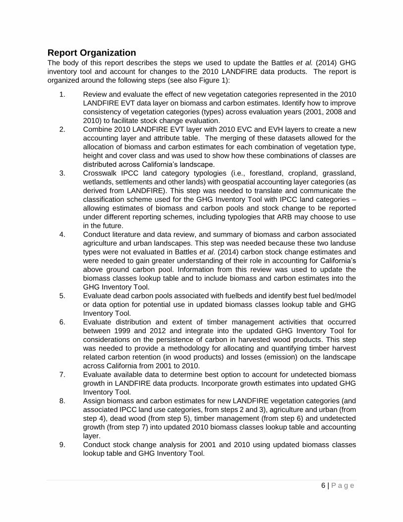
Report Organization The body of this report describes the steps we used to update the Battles et al. (2014) GHG
inventory tool and account for changes to the 2010 LANDFIRE data products. The report is
organized around the following steps (see also Figure 1):
1. Review and evaluate the effect of new vegetation categories represented in the 2010
LANDFIRE EVT data layer on biomass and carbon estimates. Identify how to improve
consistency of vegetation categories (types) across evaluation years (2001, 2008 and
2010) to facilitate stock change evaluation.
2. Combine 2010 LANDFIRE EVT layer with 2010 EVC and EVH layers to create a new
accounting layer and attribute table. The merging of these datasets allowed for the
allocation of biomass and carbon estimates for each combination of vegetation type,
height and cover class and was used to show how these combinations of classes are
distributed across California’s landscape.
3. Crosswalk IPCC land category typologies (i.e., forestland, cropland, grassland,
wetlands, settlements and other lands) with geospatial accounting layer categories (as
derived from LANDFIRE). This step was needed to translate and communicate the
classification scheme used for the GHG Inventory Tool with IPCC land categories –
allowing estimates of biomass and carbon pools and stock change to be reported
under different reporting schemes, including typologies that ARB may choose to use
in the future.
4. Conduct literature and data review, and summary of biomass and carbon associated
agriculture and urban landscapes. This step was needed because these two landuse
types were not evaluated in Battles et al. (2014) carbon stock change estimates and
were needed to gain greater understanding of their role in accounting for California’s
above ground carbon pool. Information from this review was used to update the
biomass classes lookup table and to include biomass and carbon estimates into the
GHG Inventory Tool.
5. Evaluate dead carbon pools associated with fuelbeds and identify best fuel bed/model
or data option for potential use in updated biomass classes lookup table and GHG
Inventory Tool.
6. Evaluate distribution and extent of timber management activities that occurred
between 1999 and 2012 and integrate into the updated GHG Inventory Tool for
considerations on the persistence of carbon in harvested wood products. This step
was needed to provide a methodology for allocating and quantifying timber harvest
related carbon retention (in wood products) and losses (emission) on the landscape
across California from 2001 to 2010.
7. Evaluate available data to determine best option to account for undetected biomass
growth in LANDFIRE data products. Incorporate growth estimates into updated GHG
Inventory Tool.
8. Assign biomass and carbon estimates for new LANDFIRE vegetation categories (and
associated IPCC land use categories, from steps 2 and 3), agriculture and urban (from
step 4), dead wood (from step 5), timber management (from step 6) and undetected
growth (from step 7) into updated 2010 biomass classes lookup table and accounting
layer.
9. Conduct stock change analysis for 2001 and 2010 using updated biomass classes
lookup table and GHG Inventory Tool.
7 | P a g e
Figure 1. Steps used to update Battle et al. (2014) GHG Inventory Tool.
METHODS AND RESULTS
Step 1: Review of 2010 LANDFIRE Vegetation Type Category Changes A key goal of the LANDFIRE program is to provide a consistent national vegetation map that is
sufficiently resolved to inform decisions about resource management and policy. In an effort to
remain consistent with National Vegetation Classification Standards (NVCS 2015), LANDFIRE
follows a hierarchical system with the most general category (Order) defined by the form of the
dominant vegetation: tree, shrub, herb, no dominant lifeform, and no vegetation (Table 1).
Subsequent levels include ‘class’ where the dominant vegetation is modified by its gross structure.
For example, classes within the order of ‘tree’ include ‘closed-canopy’, ‘open canopy’, and
‘sparse-tree canopy’. The ‘subclass’ divides canopy structure by leaf form. For example, the class
of closed-canopy tree is separated into ‘evergreen’, ‘deciduous’, or ‘mixed’. The most finely
resolved vegetation category is the ‘existing vegetation type’ (EVT). This LANDFIRE category is
equivalent to the sub-regional NVCS definition of a ‘group’ (Table 1), defined as: “A vegetation
classification unit of intermediate rank (6th level) defined by combinations of relatively narrow sets
of diagnostic plant species (including dominants and co-dominants), broadly similar composition,
and diagnostic growth forms that reflect biogeographic differences in mesoclimate, geology,
substrates, hydrology, and disturbance regimes (FGDC 2008).”
1. Evaluate new vegetation categories in LANDFIRE EVT, crosswalk EVTs across years
2. Combine LANDFIRE typologies for EVT, EVC and
EVH to create combined layer and attribute table
3. Cross-walk IPCC land types with combined LANDFIRE EVT,
EVH, EVH typology
4. Conduct agriculture and urban literature review,
develop summary/lookup tables for biomass and carbon
values for these landscape types
5. Evaluate options for dead carbon pool estimation
6. Identify carbon considerations of forest
management and harvested wood products
7. Evaluate FIA data to estimate undetected biomass growth in large size class trees
8. Create Access database, models and geodatabases
(i.e., updated GHG Inventory Tool) - Allocate biomass and carbon estimates via lookup tables from previous steps
9. Evaluate above ground carbon stock change (2001 to
2010)
8 | P a g e
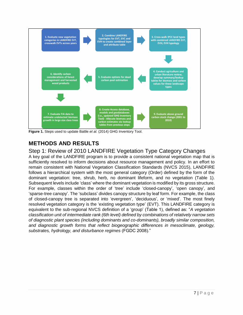
Table 1. Vegetation classification levels, classification criteria and examples of the levels of the National Vegetation
Classification Standard hierarchy for natural vegetation.1
Vegetation Classification
Level
Vegetation Classification Criteria
Ecological Context Scientific Name Common Name
Upper Levels Predominantly physiognomy
1. Formation Class
Broad combinations of general dominant growth forms.
Basic temperature (energy budget), moisture, and substrate/aquatic conditions.
Mesomorphic Tree Vegetation
Forest and Woodland
2. Formation Subclass
Combinations of general dominant and diagnostic growth forms.
Global macroclimatic factors driven primarily by latitude and continental position, or overriding substrate/aquatic conditions.
Temperate Tree Vegetation
Temperate Forest
3. Formation Combinations of dominant and diagnostic growth forms.
Global macroclimatic factors as modified by altitude, seasonality of precipitation, substrates, and hydrologic conditions.
Cool Temperate Tree Vegetation
Cool Temperate Forest
Middle Levels Physiognomy, biogeography, and floristics
4. Division Combinations of dominant and diagnostic growth forms and a broad set of diagnostic plant species that reflect biogeographic differences.
Continental differences in mesoclimate, geology, substrates, hydrology, and disturbance regimes.
Pseudotsuga - Tsuga - Picea - Pinus Forest Division
Western North America Cool Temperate Forest
5. Macrogroup Combinations of moderate sets of diagnostic plant species and diagnostic growth forms that reflect biogeographic differences.
Sub-continental to regional differences in mesoclimate, geology, substrates, hydrology, and disturbance regimes.
Pseudotsuga menziesii - Quercus garryana – Pinus ponderosa - Arbutus menziesii Macrogroup
Northern Vancouverian Montane and Foothill Forest
6. Group Combinations of relatively narrow sets of diagnostic plant species, including dominants and co-dominants, broadly similar composition, and diagnostic growth forms.
Regional mesoclimate, geology, substrates, hydrology and disturbance regimes.
Pinus ponderosa - Quercus garryana- Pseudotsuga menziesii Group
East Cascades Oak-Ponderosa Pine Forest and Woodland
Lower Levels Predominantly floristics
7. Alliance Diagnostic species, including some from the dominant growth form or layer, and moderately similar composition.
Regional to subregional climate, substrates, hydrology, moisture/ nutrient factors, and disturbance regimes.
Pinus ponderosa - Quercus garryana Woodland Alliance
Ponderosa Pine - Oregon White Oak Woodland Alliance
8. Association Diagnostic species, usually from multiple growth forms or layers, and more narrowly similar composition.
Topo-edaphic climate, substrates, hydrology, and disturbance regimes
Pinus ponderosa - Quercus garryana / Balsamorhiza sagittata Woodland
Ponderosa Pine - Oregon White Oak / Arrowleaf Balsamroot Woodland
1 Source: http://usnvc.org/data-standard/natural-vegetation-classification/
9 | P a g e
In this carbon stock assessment, we took advantage of the mesoscale resolution (As defined by
LANDFIRE) of the LANDFIRE EVT’s to assign biomass values (Battles et al. 2014). Since the
EVT is determined by the dominant vegetation, it was no surprise that EVT proved to the best
single predictor of aboveground live biomass for forests and other working lands in California.
Thus our system relies on a consistent determination of EVT as LANDFIRE updates land cover
and land use change through time. However dynamic mapping of vegetation for the entire United
States requires the means to process several hundred thousand vegetation plots and apply labels
matching the EVT definitions. By their own admission, there was limited time to evaluate the
performance of the mapping algorithms (referred to as “auto-keys”). Moreover, the baseline
LANDFIRE classification system itself has changed over time in order to match revisions to the
NVCS. As a consequence, the EVT designations are not consistent as LANDFIRE is updated
over time.
This inconsistency requires a cross-walk between EVT’s for every mapped iteration of LANDFIRE
in order to assess stock changes in carbon. Indeed we did this for the 2001 to 2008 analysis in
Battles et al. (2014) and again for the 2001 to 2010 analysis in Gonzalez et al. (2015). These
cross-walks were based on the matching descriptions of the EVT using the dominant species, the
vegetation structure, and edaphic qualifiers. Elsewhere in this report, we provide a comprehensive
crosswalk to biomass look-up tables for all EVT classes (including classes associated with
agriculture and urban landscapes) for every LANDFIRE version (2001, 2008, and 2010). Here we
explored how revisions in the LANDFIRE vegetation mapping may impact carbon stock
assessment.
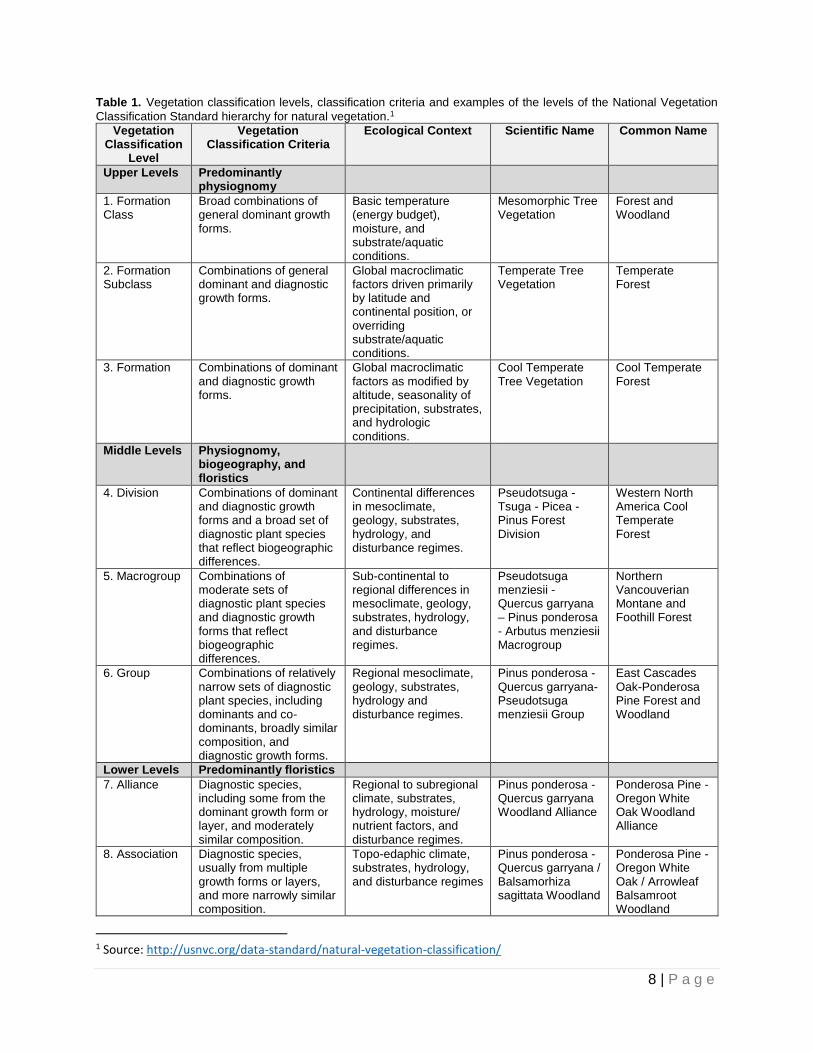
Carbon Implications of EVT Assignment. The majority of changes in LANDFIRE EVT’s are the
result of efforts to more finely resolve vegetation classes. Thus over time, there are more EVT
classes (Table 2). The reason for these fall into two categories: 1) For EVT’s with shared
dominance between deciduous and evergreen trees, the 2010 revision separated the EVT into
two classes based on tree composition and 2) for EVT’s that included more than one vegetation
structure (e.g., forest and woodland), the 2010 class was divided into two based on vegetation
structure. Other revisions were more of a book-keeping nature. For example in 2010, some EVT’s
that included the common name of the dominant species in the name were changed to the
scientific name (e.g., the Douglas-fir-Oregon White Oak Woodland became the Pseudotsuga
menziesii-Quercus garryana Woodland Alliance). While it is a chore to account for such name
changes, they will not affect the carbon estimates. In contrast, the division of EVT’s by species
composition or vegetation structure might provide more refined categories for biomass
assignments, particularly when an abundant or carbon dense EVT is split.
Table 2. Number of existing vegetation types (EVT’s) by major landuse type in California from three LANDFIRE data
iterations (2001, 2008 and 2011).
LANDFIRE Year/Versio
n
Irrigated Agriculture
Urban Forests and
Working Lands
Total
2001 9 10 138 158
2008 16 10 141 168
2010 30 19 154 204
10 | P a g e
A good test case for California is the “California Lower Montane Blue Oak-Foothill Pine Woodland
and Savanna” (i.e., blue oak woodlands). It is an example of an EVT that was split into three
separate EVT’s in 2010 based on compositional differences (oak dominance versus pine
dominance) and structure (forest/woodland versus savanna). It is the second most common
vegetation type (by area) in the state covering 16,740 km2 and accounting for 8% of the above-
ground carbon stock (based on 2008 LANDFIRE - urban and irrigated agricultural lands excluded,
Battles et al. 2014). Based on FIA plot data for this EVT (277 plots), carbon density varies by an
order of magnitude. Below three specific objectives are outlined to quantify the carbon
implications of the revisions to the blue oak woodland EVT.
Objective 1 - The EVT Classification Process. In 2010, LANDFIRE divided the blue oak woodland
into three separate EVT’s: California Lower Montane Blue Oak Forest and Woodland, California
Lower Montane Blue Oak-Foothill Pine Forest and Woodland, California Lower Montane Foothill
Pine Woodland and Savanna. This revision relies on the LANDFIRE mapping algorithm (auto key)
to parse the previous EVT into a more tree-centric, oak dominated class from a more open,
savanna class dominated by pines while also retaining a mixed species designations for the sites
in the middle of this gradient. LANDFIRE 2010 adopted these divisions even though the
NatureServe analysis on mapping accuracy specifically notes the difficulty of distinguishing
floristically similar ecological systems and the gains in accuracy associated with slightly coarser
vegetation classes (NatureServe 2012). Indeed, the auto key results for the coarser 2008 EVT
matched expert opinion 84% of the time (42 correct out of 50, NatureServe 2012). There was no
accuracy assessment conducted for the revised 2010 LANDFIRE EVT’s.
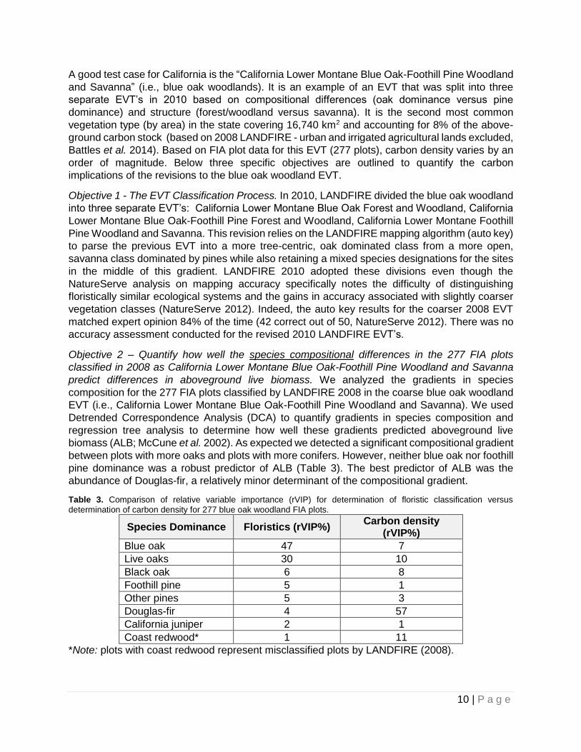
Objective 2 – Quantify how well the species compositional differences in the 277 FIA plots
classified in 2008 as California Lower Montane Blue Oak-Foothill Pine Woodland and Savanna
predict differences in aboveground live biomass. We analyzed the gradients in species
composition for the 277 FIA plots classified by LANDFIRE 2008 in the coarse blue oak woodland
EVT (i.e., California Lower Montane Blue Oak-Foothill Pine Woodland and Savanna). We used
Detrended Correspondence Analysis (DCA) to quantify gradients in species composition and
regression tree analysis to determine how well these gradients predicted aboveground live
biomass (ALB; McCune et al. 2002). As expected we detected a significant compositional gradient
between plots with more oaks and plots with more conifers. However, neither blue oak nor foothill
pine dominance was a robust predictor of ALB (Table 3). The best predictor of ALB was the
abundance of Douglas-fir, a relatively minor determinant of the compositional gradient.
Table 3. Comparison of relative variable importance (rVIP) for determination of floristic classification versus
determination of carbon density for 277 blue oak woodland FIA plots.
Species Dominance Floristics (rVIP%) Carbon density
(rVIP%)
Blue oak 47 7
Live oaks 30 10
Black oak 6 8
Foothill pine 5 1
Other pines 5 3
Douglas-fir 4 57
California juniper 2 1
Coast redwood* 1 11
*Note: plots with coast redwood represent misclassified plots by LANDFIRE (2008).
11 | P a g e
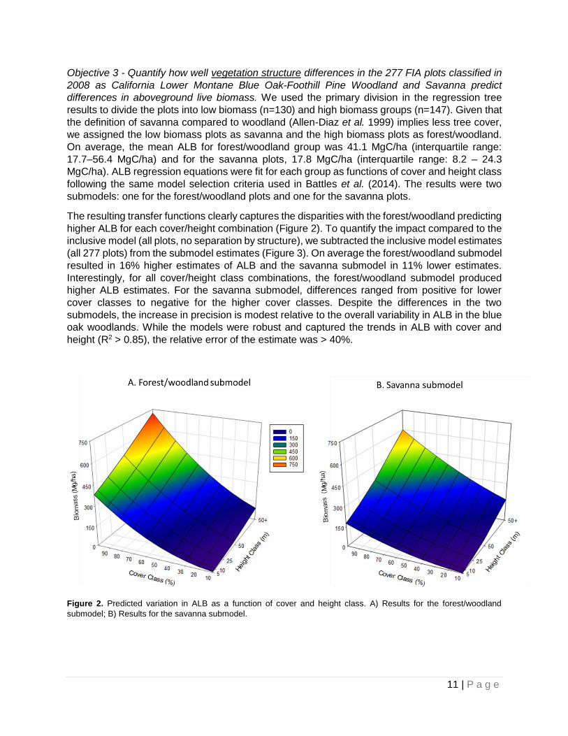
Objective 3 - Quantify how well vegetation structure differences in the 277 FIA plots classified in
2008 as California Lower Montane Blue Oak-Foothill Pine Woodland and Savanna predict
differences in aboveground live biomass. We used the primary division in the regression tree
results to divide the plots into low biomass (n=130) and high biomass groups (n=147). Given that
the definition of savanna compared to woodland (Allen-Diaz et al. 1999) implies less tree cover,
we assigned the low biomass plots as savanna and the high biomass plots as forest/woodland.
On average, the mean ALB for forest/woodland group was 41.1 MgC/ha (interquartile range:
17.7–56.4 MgC/ha) and for the savanna plots, 17.8 MgC/ha (interquartile range: 8.2 – 24.3
MgC/ha). ALB regression equations were fit for each group as functions of cover and height class
following the same model selection criteria used in Battles et al. (2014). The results were two
submodels: one for the forest/woodland plots and one for the savanna plots.
The resulting transfer functions clearly captures the disparities with the forest/woodland predicting
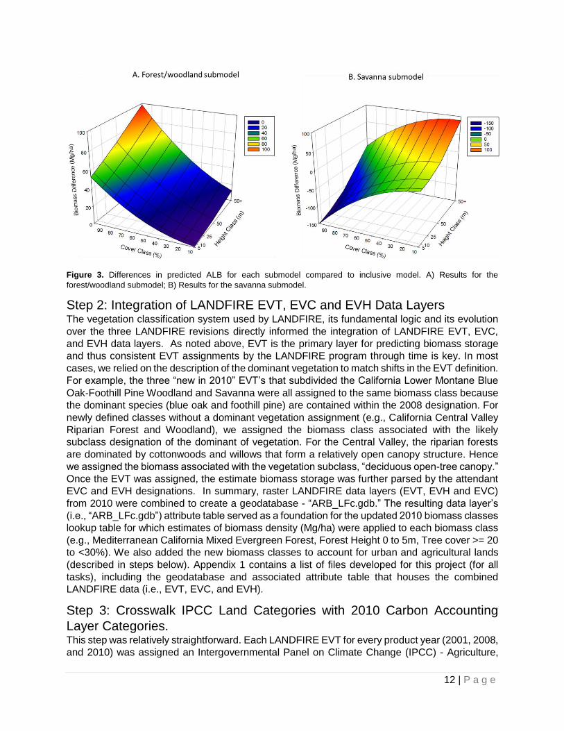
higher ALB for each cover/height combination (Figure 2). To quantify the impact compared to the
inclusive model (all plots, no separation by structure), we subtracted the inclusive model estimates
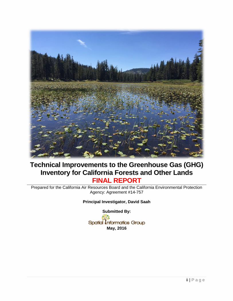
(all 277 plots) from the submodel estimates (Figure 3). On average the forest/woodland submodel
resulted in 16% higher estimates of ALB and the savanna submodel in 11% lower estimates.
Interestingly, for all cover/height class combinations, the forest/woodland submodel produced
higher ALB estimates. For the savanna submodel, differences ranged from positive for lower
cover classes to negative for the higher cover classes. Despite the differences in the two
submodels, the increase in precision is modest relative to the overall variability in ALB in the blue
oak woodlands. While the models were robust and captured the trends in ALB with cover and
height (R2 > 0.85), the relative error of the estimate was > 40%.
Figure 2. Predicted variation in ALB as a function of cover and height class. A) Results for the forest/woodland
submodel; B) Results for the savanna submodel.
12 | P a g e
Figure 3. Differences in predicted ALB for each submodel compared to inclusive model. A) Results for the
forest/woodland submodel; B) Results for the savanna submodel.
Step 2: Integration of LANDFIRE EVT, EVC and EVH Data Layers The vegetation classification system used by LANDFIRE, its fundamental logic and its evolution
over the three LANDFIRE revisions directly informed the integration of LANDFIRE EVT, EVC,
and EVH data layers. As noted above, EVT is the primary layer for predicting biomass storage
and thus consistent EVT assignments by the LANDFIRE program through time is key. In most
cases, we relied on the description of the dominant vegetation to match shifts in the EVT definition.
For example, the three “new in 2010” EVT’s that subdivided the California Lower Montane Blue
Oak‐Foothill Pine Woodland and Savanna were all assigned to the same biomass class because
the dominant species (blue oak and foothill pine) are contained within the 2008 designation. For
newly defined classes without a dominant vegetation assignment (e.g., California Central Valley
Riparian Forest and Woodland), we assigned the biomass class associated with the likely
subclass designation of the dominant of vegetation. For the Central Valley, the riparian forests
are dominated by cottonwoods and willows that form a relatively open canopy structure. Hence
we assigned the biomass associated with the vegetation subclass, “deciduous open-tree canopy.”
Once the EVT was assigned, the estimate biomass storage was further parsed by the attendant
EVC and EVH designations. In summary, raster LANDFIRE data layers (EVT, EVH and EVC)
from 2010 were combined to create a geodatabase - “ARB_LFc.gdb.” The resulting data layer’s
(i.e., “ARB_LFc.gdb”) attribute table served as a foundation for the updated 2010 biomass classes
lookup table for which estimates of biomass density (Mg/ha) were applied to each biomass class
(e.g., Mediterranean California Mixed Evergreen Forest, Forest Height 0 to 5m, Tree cover >= 20
to <30%). We also added the new biomass classes to account for urban and agricultural lands
(described in steps below). Appendix 1 contains a list of files developed for this project (for all
tasks), including the geodatabase and associated attribute table that houses the combined
LANDFIRE data (i.e., EVT, EVC, and EVH).
Step 3: Crosswalk IPCC Land Categories with 2010 Carbon Accounting
Layer Categories. This step was relatively straightforward. Each LANDFIRE EVT for every product year (2001, 2008,
and 2010) was assigned an Intergovernmental Panel on Climate Change (IPCC) - Agriculture,
13 | P a g e
Forestry and Other Land Use (AFOLU) category based on the description of the existing
vegetation. Corresponding IPCC AFOLU categories and LANDFIRE vegetation type categories
(as combined in step 2 with EVC and EVH) were aligned based on their respective definitions and
organized into a crosswalk table (“BATTLES_Biomass-LUT_01-08-10_20151029”) in the
“ARB_C_LUT_v2.7.accdb” database to facilitate queries for either land typology.
Step 4: Literature and Data Review and Summary of Biomass and Carbon
Associated Agriculture and Urban Landscapes.
Agriculture and Urban Vegetation Types We conducted an extensive review of best available science to construct estimates of above
ground carbon stocks with associated agriculture and urban landscapes. Literature and data
sources consulted included: Google Scholar, Web of Science, UC Agricultural Extension, and
local agricultural cooperatives. A Microsoft Access database titled “ARB literature review
database” was used to organize summarized information including a complete the list of
information sources (see Appendix 2) Biomass and carbon estimates extracted from reviewed
information are organized into an updated biomass classes lookup table and categorized into one
of the corresponding LANDFIRE Existing Vegetation Types associated with agricultural or other
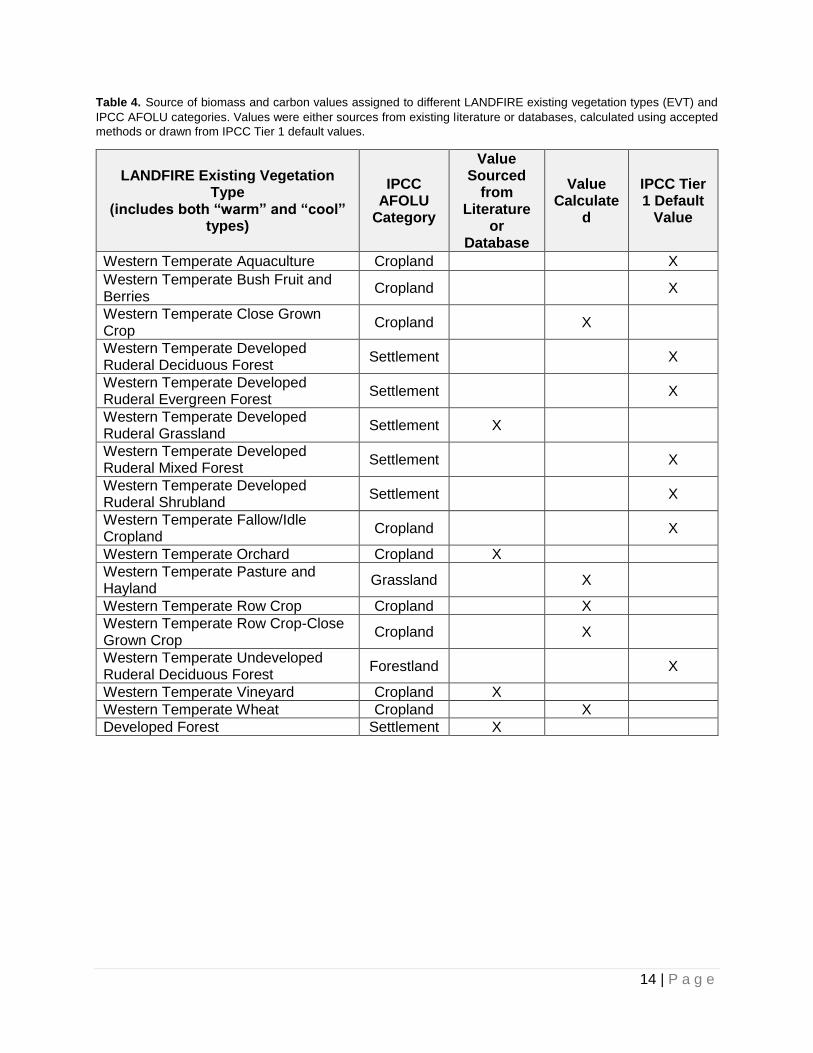
developed lands, as well as into corresponding IPCC AFOLU categories (Table 4).
LANDFIRE EVTs for agriculture and urban vegetation categories occur as both “Western Cool
Temperate” and “Western Warm Temperate” within California. In most cases, it was not possible
to distinguish biomass or carbon stock values in warm vs. cool types, so except where noted the
same values are used for each. For some LANDFIRE EVTs, a single value was obtained or
calculated to use in the statewide lookup table. Where multiple crop types comprised a LANDFIRE
EVT, the values were weighted based on acreage summaries available through the ‘CropScape’
database (Boryan et al. 2011).
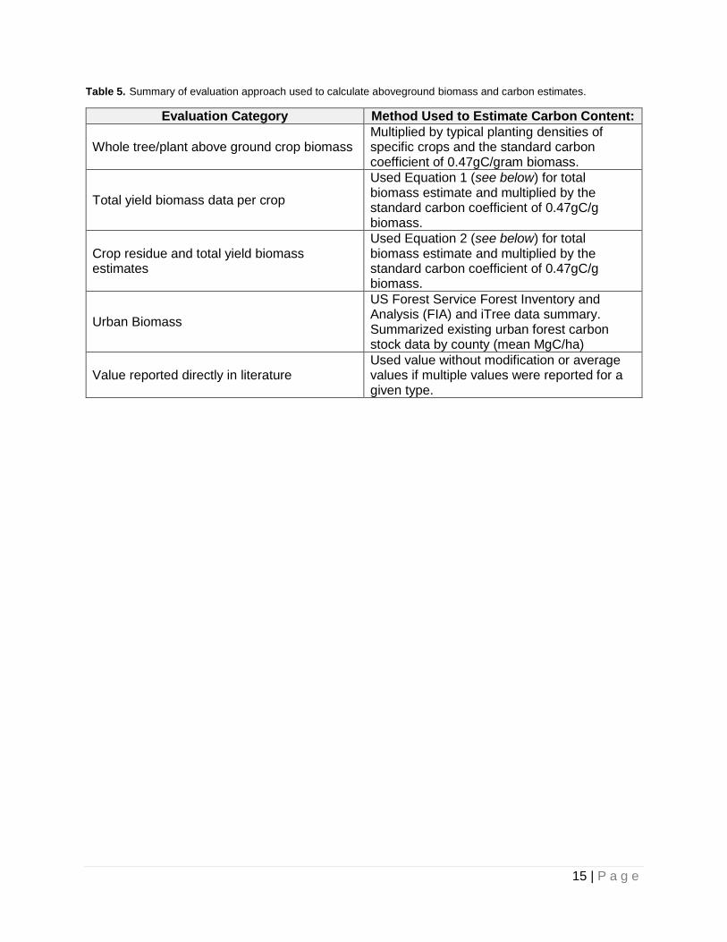
Biomass and Carbon Stock Value Calculation Methods We used five different methods to summarize and estimate biomass and calculate carbon (C) content as the data were presented in different ways in the literature and in relevant databases. Different methods were required because we did not find total tree or plant biomass estimates nor were essential carbon equation parameters available on every crop grown in the state. Table 5 summarizes the general approaches used to quantifying total aboveground biomass for each LANDFIRE EVT. A detailed description of each method as it applies to the LANDFIRE EVT follows. Data sources varied from published literature to online databases (see Appendix 2 for list of information sources).
Vineyard and Orchard Existing Vegetation Types
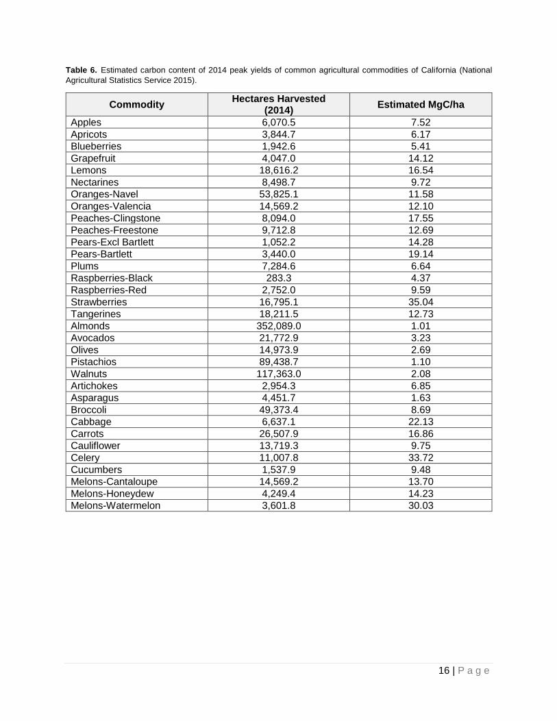
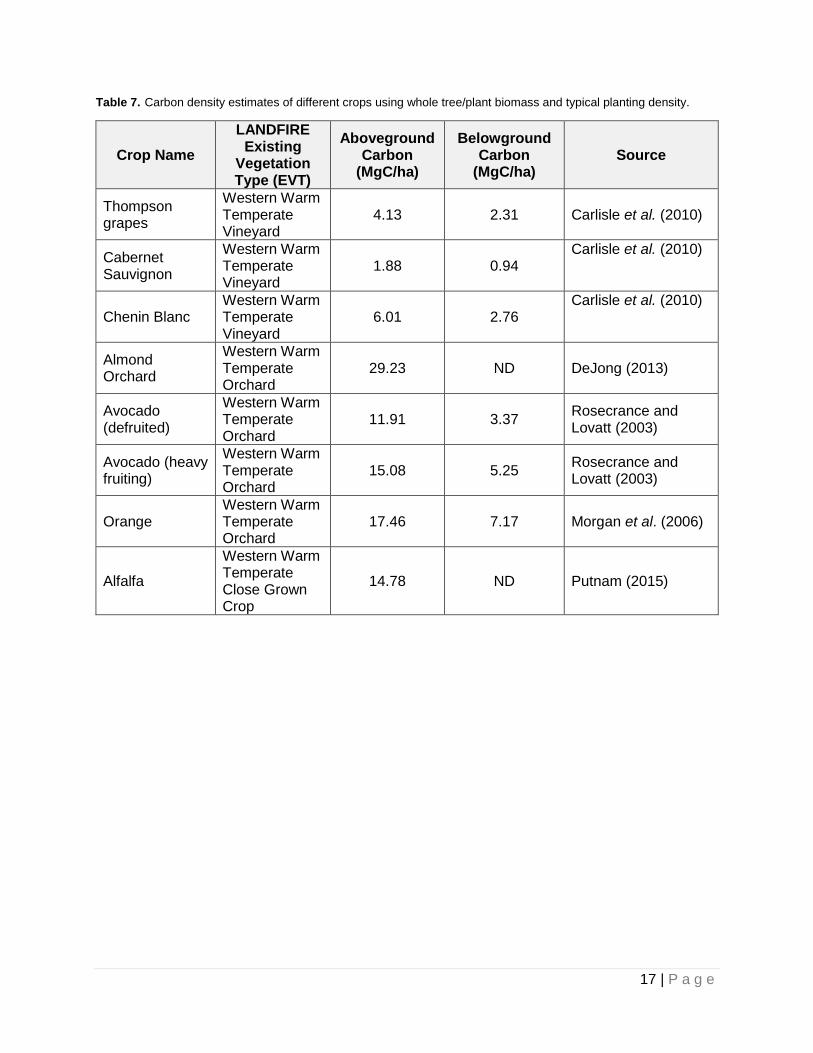
Vineyard and orchard EVTs included almonds, avocadoes, oranges, and grapes (Table 6).
Estimates of the carbon content of almond (DeJong 2013), orange (Morgan et al. 2006), and
avocado (Rosecrance and Lovatt 2003), orchards and grape vineyards (Carlisle et al. 2010) were
made using published data on whole tree or vine biomass estimates, and multiplied by typical
planting densities of given species (trees/hectare), and the standard carbon coefficient of
0.47gC/g biomass (McGroddy et al. 2004). These were the only crops where this type of data
were found and estimated in this way (see also Table 7).
14 | P a g e
Table 4. Source of biomass and carbon values assigned to different LANDFIRE existing vegetation types (EVT) and
IPCC AFOLU categories. Values were either sources from existing literature or databases, calculated using accepted
methods or drawn from IPCC Tier 1 default values.
LANDFIRE Existing Vegetation Type
(includes both “warm” and “cool” types)
IPCC AFOLU
Category
Value Sourced
from Literature
or Database
Value Calculate
d
IPCC Tier 1 Default
Value
Western Temperate Aquaculture Cropland X
Western Temperate Bush Fruit and Berries
Cropland X
Western Temperate Close Grown Crop
Cropland X
Western Temperate Developed Ruderal Deciduous Forest
Settlement X
Western Temperate Developed Ruderal Evergreen Forest
Settlement X
Western Temperate Developed Ruderal Grassland
Settlement X
Western Temperate Developed Ruderal Mixed Forest
Settlement X
Western Temperate Developed Ruderal Shrubland
Settlement X
Western Temperate Fallow/Idle Cropland
Cropland X
Western Temperate Orchard Cropland X
Western Temperate Pasture and Hayland
Grassland X
Western Temperate Row Crop Cropland X
Western Temperate Row Crop-Close Grown Crop
Cropland X
Western Temperate Undeveloped Ruderal Deciduous Forest
Forestland X
Western Temperate Vineyard Cropland X
Western Temperate Wheat Cropland X
Developed Forest Settlement X
15 | P a g e
Table 5. Summary of evaluation approach used to calculate aboveground biomass and carbon estimates.
Evaluation Category Method Used to Estimate Carbon Content:
Whole tree/plant above ground crop biomass Multiplied by typical planting densities of specific crops and the standard carbon coefficient of 0.47gC/gram biomass.
Total yield biomass data per crop
Used Equation 1 (see below) for total biomass estimate and multiplied by the standard carbon coefficient of 0.47gC/g biomass.
Crop residue and total yield biomass estimates
Used Equation 2 (see below) for total biomass estimate and multiplied by the standard carbon coefficient of 0.47gC/g biomass.
Urban Biomass
US Forest Service Forest Inventory and Analysis (FIA) and iTree data summary. Summarized existing urban forest carbon stock data by county (mean MgC/ha)
Value reported directly in literature Used value without modification or average values if multiple values were reported for a given type.
16 | P a g e
Table 6. Estimated carbon content of 2014 peak yields of common agricultural commodities of California (National
Agricultural Statistics Service 2015).
Commodity Hectares Harvested
(2014) Estimated MgC/ha
Apples 6,070.5 7.52
Apricots 3,844.7 6.17
Blueberries 1,942.6 5.41
Grapefruit 4,047.0 14.12
Lemons 18,616.2 16.54
Nectarines 8,498.7 9.72
Oranges-Navel 53,825.1 11.58
Oranges-Valencia 14,569.2 12.10
Peaches-Clingstone 8,094.0 17.55
Peaches-Freestone 9,712.8 12.69
Pears-Excl Bartlett 1,052.2 14.28
Pears-Bartlett 3,440.0 19.14
Plums 7,284.6 6.64
Raspberries-Black 283.3 4.37
Raspberries-Red 2,752.0 9.59
Strawberries 16,795.1 35.04
Tangerines 18,211.5 12.73
Almonds 352,089.0 1.01
Avocados 21,772.9 3.23
Olives 14,973.9 2.69
Pistachios 89,438.7 1.10
Walnuts 117,363.0 2.08
Artichokes 2,954.3 6.85
Asparagus 4,451.7 1.63
Broccoli 49,373.4 8.69
Cabbage 6,637.1 22.13
Carrots 26,507.9 16.86
Cauliflower 13,719.3 9.75
Celery 11,007.8 33.72
Cucumbers 1,537.9 9.48
Melons-Cantaloupe 14,569.2 13.70
Melons-Honeydew 4,249.4 14.23
Melons-Watermelon 3,601.8 30.03
17 | P a g e
Table 7. Carbon density estimates of different crops using whole tree/plant biomass and typical planting density.
Crop Name
LANDFIRE Existing
Vegetation Type (EVT)
Aboveground Carbon
(MgC/ha)
Belowground Carbon
(MgC/ha) Source
Thompson grapes
Western Warm Temperate Vineyard
4.13 2.31 Carlisle et al. (2010)
Cabernet Sauvignon
Western Warm Temperate Vineyard
1.88 0.94 Carlisle et al. (2010)
Chenin Blanc Western Warm Temperate Vineyard
6.01 2.76 Carlisle et al. (2010)
Almond Orchard
Western Warm Temperate Orchard
29.23 ND DeJong (2013)
Avocado (defruited)
Western Warm Temperate Orchard
11.91 3.37 Rosecrance and Lovatt (2003)
Avocado (heavy fruiting)
Western Warm Temperate Orchard
15.08 5.25 Rosecrance and Lovatt (2003)
Orange Western Warm Temperate Orchard
17.46 7.17 Morgan et al. (2006)
Alfalfa
Western Warm Temperate Close Grown Crop
14.78 ND Putnam (2015)

18 | P a g e
Close Grown Crop EVT, Row Crop EVT, Row Crop-Close Grown Crop EVT
Close grown crop types included Alfalfa, Rice, Oats, and Barley. Biomass and carbon values were
weighted based on the statewide acreage allocation of each crop type. A single weighted carbon
stock value was then used for the statewide lookup table. Row crops included:
Tomatoes Cotton Corn Sunflowers
Safflower Triticale Clover/Wildflowers Onions
Double Crop Winter Wheat/Sorghum
Dry Beans Sugar beets Potatoes
Misc. Vegetables & Fruits
Carrots Garlic Lettuce
Other Crops Rye Cantaloupe Greens
Sorghum Watermelons Peas Broccoli
Pumpkins Herbs Honeydew Melons Sweet Corn
Asparagus Peppers Double Crop
Lettuce/Durum Wheat
Squash
Mint Sweet Potatoes Cabbage Vetch
Double Crop Lettuce/Cantaloupe
Canola Cauliflower Double Crop
Lettuce/Cotton
Double Crop Winter Wheat/Cotton
Sugarcane Cucumbers Radishes
Pop or Orn Corn Other Small
Grains Double Crop
Lettuce/Barley Eggplants
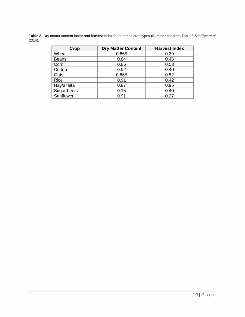
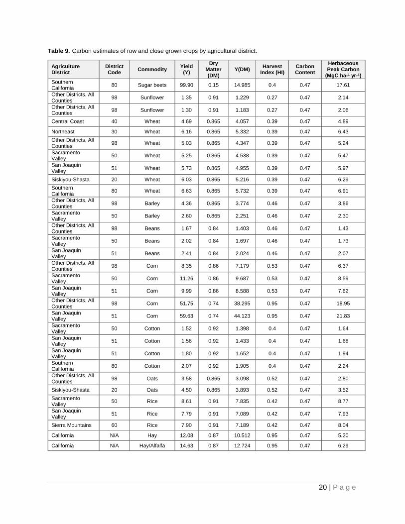
Total above ground yield of crop (for barley, corn, sorghum, sugar beets, cotton, oats, beans, rice, sunflower, wheat and soybean) or peak forage (hay and alfalfa) yield for grazing lands (metric tons biomass/hectare) was needed to calculate above ground C stocks. We used Equation 1 (below) and Table 8 below (Eve et al. 2014, adapted from West et al. 2010) to provide a method to convert crop yield to C stocks. The approach was discussed with Mark Easter of the Natural Resource Ecology Laboratory at Colorado State University, who has experience working with similar data and calculations for IPCC reports. Mr. Easter affirmed the approach was appropriate for developing peak herbaceous carbon stock values (Table 9).
Equation 1. The following equation used to calculate aboveground herbaceous biomass carbon
stock for harvested crops (adapted from Eve et al. 2014 - Equation 3-3).
𝐻𝑃𝑒𝑎𝑘 = (𝑌𝑑𝑚
𝐻𝐼⁄ ) × 𝐶
Where:
HPeak = Annual peak above ground herbaceous (H) biomass carbon stock (metric tons C ha-1 year-1)
Ydm = Crop harvest or forage yield (Y), corrected for dry matter (dm) content (metric tons C ha-1 year-1); dry matter content of harvested crop biomass or forage is dimensionless and derived from Table 8 below.
HI = Harvest Index (dimensionless, from Table 8 below)
C = Carbon fraction of above ground biomass (0.47 gC/g biomass assumed) Yield (e.g., in bushels per acre) was obtained for each county in California from a query of the National Agricultural Statistics Service (NASS, http://quickstats.nass.usda.gov/).
19 | P a g e
Table 8. Dry matter content factor and harvest Index for common crop types (Summarized from Table 3-5 in Eve et al.
2014).
Crop Dry Matter Content Harvest Index
Wheat 0.865 0.39
Beans 0.84 0.46
Corn 0.86 0.53
Cotton 0.92 0.40
Oats 0.865 0.52
Rice 0.91 0.42
Hay/alfalfa 0.87 0.95
Sugar beets 0.15 0.40
Sunflower 0.91 0.27
20 | P a g e
Table 9. Carbon estimates of row and close grown crops by agricultural district.
Agriculture District
District Code
Commodity Yield (Y)
Dry Matter (DM)
Y(DM) Harvest
Index (HI) Carbon Content
Herbaceous Peak Carbon
(MgC ha-¹ yr-¹)
Southern California
80 Sugar beets 99.90 0.15 14.985 0.4 0.47 17.61
Other Districts, All Counties
98 Sunflower 1.35 0.91 1.229 0.27 0.47 2.14
Other Districts, All Counties
98 Sunflower 1.30 0.91 1.183 0.27 0.47 2.06
Central Coast 40 Wheat 4.69 0.865 4.057 0.39 0.47 4.89
Northeast 30 Wheat 6.16 0.865 5.332 0.39 0.47 6.43
Other Districts, All Counties
98 Wheat 5.03 0.865 4.347 0.39 0.47 5.24
Sacramento Valley
50 Wheat 5.25 0.865 4.538 0.39 0.47 5.47
San Joaquin Valley
51 Wheat 5.73 0.865 4.955 0.39 0.47 5.97
Siskiyou-Shasta 20 Wheat 6.03 0.865 5.216 0.39 0.47 6.29
Southern California
80 Wheat 6.63 0.865 5.732 0.39 0.47 6.91
Other Districts, All Counties
98 Barley 4.36 0.865 3.774 0.46 0.47 3.86
Sacramento Valley
50 Barley 2.60 0.865 2.251 0.46 0.47 2.30
Other Districts, All Counties
98 Beans 1.67 0.84 1.403 0.46 0.47 1.43
Sacramento Valley
50 Beans 2.02 0.84 1.697 0.46 0.47 1.73
San Joaquin Valley
51 Beans 2.41 0.84 2.024 0.46 0.47 2.07
Other Districts, All Counties
98 Corn 8.35 0.86 7.179 0.53 0.47 6.37
Sacramento Valley
50 Corn 11.26 0.86 9.687 0.53 0.47 8.59
San Joaquin Valley
51 Corn 9.99 0.86 8.588 0.53 0.47 7.62
Other Districts, All Counties
98 Corn 51.75 0.74 38.295 0.95 0.47 18.95
San Joaquin Valley
51 Corn 59.63 0.74 44.123 0.95 0.47 21.83
Sacramento Valley
50 Cotton 1.52 0.92 1.398 0.4 0.47 1.64
San Joaquin Valley
51 Cotton 1.56 0.92 1.433 0.4 0.47 1.68
San Joaquin Valley
51 Cotton 1.80 0.92 1.652 0.4 0.47 1.94
Southern California
80 Cotton 2.07 0.92 1.905 0.4 0.47 2.24
Other Districts, All Counties
98 Oats 3.58 0.865 3.098 0.52 0.47 2.80
Siskiyou-Shasta 20 Oats 4.50 0.865 3.893 0.52 0.47 3.52
Sacramento Valley
50 Rice 8.61 0.91 7.835 0.42 0.47 8.77
San Joaquin Valley
51 Rice 7.79 0.91 7.089 0.42 0.47 7.93
Sierra Mountains 60 Rice 7.90 0.91 7.189 0.42 0.47 8.04
California N/A Hay 12.08 0.87 10.512 0.95 0.47 5.20
California N/A Hay/Alfalfa 14.63 0.87 12.724 0.95 0.47 6.29
21 | P a g e
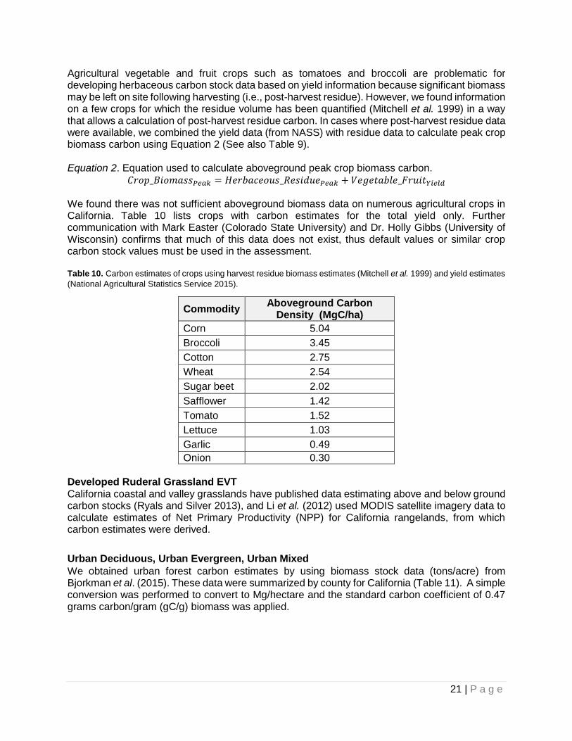
Agricultural vegetable and fruit crops such as tomatoes and broccoli are problematic for developing herbaceous carbon stock data based on yield information because significant biomass may be left on site following harvesting (i.e., post-harvest residue). However, we found information on a few crops for which the residue volume has been quantified (Mitchell et al. 1999) in a way that allows a calculation of post-harvest residue carbon. In cases where post-harvest residue data were available, we combined the yield data (from NASS) with residue data to calculate peak crop biomass carbon using Equation 2 (See also Table 9). Equation 2. Equation used to calculate aboveground peak crop biomass carbon.
𝐶𝑟𝑜𝑝_𝐵𝑖𝑜𝑚𝑎𝑠𝑠𝑃𝑒𝑎𝑘 = 𝐻𝑒𝑟𝑏𝑎𝑐𝑒𝑜𝑢𝑠_𝑅𝑒𝑠𝑖𝑑𝑢𝑒𝑃𝑒𝑎𝑘 + 𝑉𝑒𝑔𝑒𝑡𝑎𝑏𝑙𝑒_𝐹𝑟𝑢𝑖𝑡𝑌𝑖𝑒𝑙𝑑 We found there was not sufficient aboveground biomass data on numerous agricultural crops in California. Table 10 lists crops with carbon estimates for the total yield only. Further communication with Mark Easter (Colorado State University) and Dr. Holly Gibbs (University of Wisconsin) confirms that much of this data does not exist, thus default values or similar crop carbon stock values must be used in the assessment. Table 10. Carbon estimates of crops using harvest residue biomass estimates (Mitchell et al. 1999) and yield estimates
(National Agricultural Statistics Service 2015).
Commodity Aboveground Carbon
Density (MgC/ha)
Corn 5.04
Broccoli 3.45
Cotton 2.75
Wheat 2.54
Sugar beet 2.02
Safflower 1.42
Tomato 1.52
Lettuce 1.03
Garlic 0.49
Onion 0.30
Developed Ruderal Grassland EVT California coastal and valley grasslands have published data estimating above and below ground carbon stocks (Ryals and Silver 2013), and Li et al. (2012) used MODIS satellite imagery data to calculate estimates of Net Primary Productivity (NPP) for California rangelands, from which carbon estimates were derived.
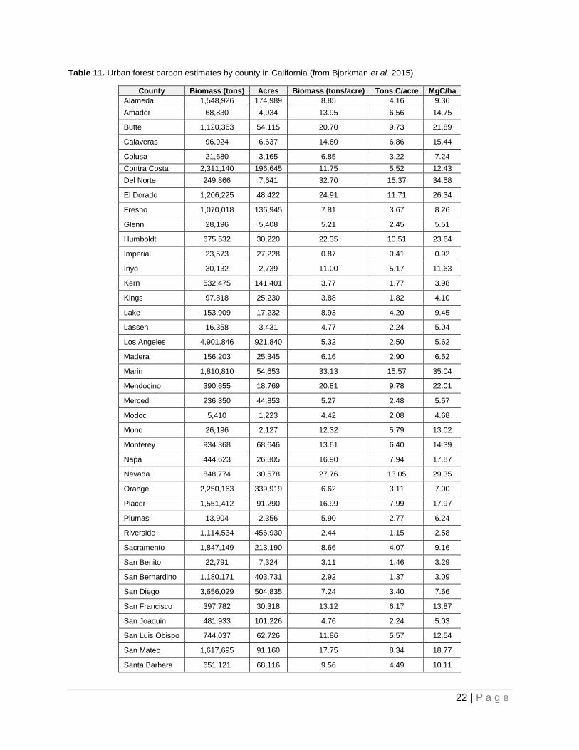
Urban Deciduous, Urban Evergreen, Urban Mixed
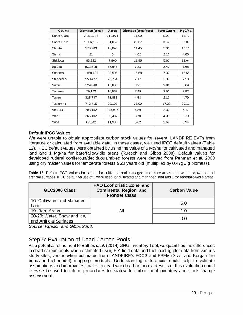
We obtained urban forest carbon estimates by using biomass stock data (tons/acre) from Bjorkman et al. (2015). These data were summarized by county for California (Table 11). A simple conversion was performed to convert to Mg/hectare and the standard carbon coefficient of 0.47 grams carbon/gram (gC/g) biomass was applied.
22 | P a g e
Table 11. Urban forest carbon estimates by county in California (from Bjorkman et al. 2015).
County Biomass (tons) Acres Biomass (tons/acre) Tons C/acre MgC/ha
Alameda 1,548,926 174,989 8.85 4.16 9.36
Amador 68,830 4,934 13.95 6.56 14.75
Butte 1,120,363 54,115 20.70 9.73 21.89
Calaveras 96,924 6,637 14.60 6.86 15.44
Colusa 21,680 3,165 6.85 3.22 7.24
Contra Costa 2,311,140 196,645 11.75 5.52 12.43
Del Norte 249,866 7,641 32.70 15.37 34.58
El Dorado 1,206,225 48,422 24.91 11.71 26.34
Fresno 1,070,018 136,945 7.81 3.67 8.26
Glenn 28,196 5,408 5.21 2.45 5.51
Humboldt 675,532 30,220 22.35 10.51 23.64
Imperial 23,573 27,228 0.87 0.41 0.92
Inyo 30,132 2,739 11.00 5.17 11.63
Kern 532,475 141,401 3.77 1.77 3.98
Kings 97,818 25,230 3.88 1.82 4.10
Lake 153,909 17,232 8.93 4.20 9.45
Lassen 16,358 3,431 4.77 2.24 5.04
Los Angeles 4,901,846 921,840 5.32 2.50 5.62
Madera 156,203 25,345 6.16 2.90 6.52
Marin 1,810,810 54,653 33.13 15.57 35.04
Mendocino 390,655 18,769 20.81 9.78 22.01
Merced 236,350 44,853 5.27 2.48 5.57
Modoc 5,410 1,223 4.42 2.08 4.68
Mono 26,196 2,127 12.32 5.79 13.02
Monterey 934,368 68,646 13.61 6.40 14.39
Napa 444,623 26,305 16.90 7.94 17.87
Nevada 848,774 30,578 27.76 13.05 29.35
Orange 2,250,163 339,919 6.62 3.11 7.00
Placer 1,551,412 91,290 16.99 7.99 17.97
Plumas 13,904 2,356 5.90 2.77 6.24
Riverside 1,114,534 456,930 2.44 1.15 2.58
Sacramento 1,847,149 213,190 8.66 4.07 9.16
San Benito 22,791 7,324 3.11 1.46 3.29
San Bernardino 1,180,171 403,731 2.92 1.37 3.09
San Diego 3,656,029 504,835 7.24 3.40 7.66
San Francisco 397,782 30,318 13.12 6.17 13.87
San Joaquin 481,933 101,226 4.76 2.24 5.03
San Luis Obispo 744,037 62,726 11.86 5.57 12.54
San Mateo 1,617,695 91,160 17.75 8.34 18.77
Santa Barbara 651,121 68,116 9.56 4.49 10.11
23 | P a g e
County Biomass (tons) Acres Biomass (tons/acre) Tons C/acre MgC/ha
Santa Clara 2,351,202 211,971 11.09 5.21 11.73
Santa Cruz 1,356,195 51,052 26.57 12.49 28.09
Shasta 570,789 49,843 11.45 5.38 12.11
Sierra 21 5 4.62 2.17 4.88
Siskiyou 93,922 7,860 11.95 5.62 12.64
Solano 532,515 73,643 7.23 3.40 7.65
Sonoma 1,450,695 92,505 15.68 7.37 16.58
Stanislaus 550,427 76,754 7.17 3.37 7.58
Sutter 129,849 15,808 8.21 3.86 8.69
Tehama 79,142 10,568 7.49 3.52 7.92
Tulare 325,787 71,885 4.53 2.13 4.79
Tuolumne 743,715 20,108 36.99 17.38 39.11
Ventura 703,152 143,916 4.89 2.30 5.17
Yolo 265,102 30,487 8.70 4.09 9.20
Yuba 67,342 11,986 5.62 2.64 5.94
Default IPCC Values We were unable to obtain appropriate carbon stock values for several LANDFIRE EVTs from literature or calculated from available data. In those cases, we used IPCC default values (Table 12). IPCC default values were obtained by using the value of 5 Mg/ha for cultivated and managed land and 1 Mg/ha for bare/fallow/idle areas (Ruesch and Gibbs 2008). Default values for developed ruderal coniferous/deciduous/mixed forests were derived from Penman et al. 2003 using dry matter values for temperate forests ≤ 20 years old (multiplied by 0.47gC/g biomass). Table 12. Default IPCC Values for carbon for cultivated and managed land, bare areas, and water, snow, ice and
artificial surfaces. IPCC default values of 5 were used for cultivated and managed land and 1 for bare/fallow/idle areas.
GLC2000 Class FAO Ecofloristic Zone, and
Continental Region, and Frontier Class
Carbon Value
16: Cultivated and Managed Land
All
5.0
19: Bare Areas 1.0
20-23: Water, Snow and Ice, and Artificial Surfaces
0.0
Source: Ruesch and Gibbs 2008.
Step 5: Evaluation of Dead Carbon Pools As a potential refinement to Battles et al. (2014) GHG Inventory Tool, we quantified the differences in dead carbon pools when estimated using FIA field data and fuel loading plot data from various study sites, versus when estimated from LANDFIRE’s FCCS and FBFM (Scott and Burgan fire behavior fuel model) mapping products. Understanding differences could help to validate assumptions and improve estimates in dead wood carbon pools. Results of this evaluation could likewise be used to inform procedures for statewide carbon pool inventory and stock change assessment.
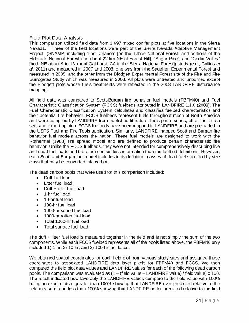
24 | P a g e
Field Plot Data Analysis This comparison utilized field data from 1,697 mixed conifer plots at five locations in the Sierra Nevada. Three of the field locations were part of the Sierra Nevada Adaptive Management Project (SNAMP; including “Last Chance” [on the Tahoe National Forest, and portions of the Eldorado National Forest and about 22 km NE of Forest Hill], “Sugar Pine”, and “Cedar Valley” [both NE about 9 to 13 km of Oakhurst, CA in the Sierra National Forest]) study (e.g., Collins et al. 2011) and measured in 2007 and 2008, one was from the Sagehen Experimental Forest and measured in 2005, and the other from the Blodgett Experimental Forest site of the Fire and Fire Surrogates Study which was measured in 2003. All plots were untreated and unburned except the Blodgett plots whose fuels treatments were reflected in the 2008 LANDFIRE disturbance mapping. All field data was compared to Scott-Burgan fire behavior fuel models (FBFM40) and Fuel Characteristic Classification System (FCCS) fuelbeds attributed in LANDFIRE 1.1.0 (2008). The Fuel Characteristic Classification System calculates and classifies fuelbed characteristics and their potential fire behavior. FCCS fuelbeds represent fuels throughout much of North America and were compiled by LANDFIRE from published literature, fuels photo series, other fuels data sets and expert opinion. FCCS fuelbeds have been mapped in LANDFIRE and are preloaded in the USFS Fuel and Fire Tools application. Similarly, LANDFIRE mapped Scott and Burgan fire behavior fuel models across the nation. These fuel models are designed to work with the Rothermel (1983) fire spread model and are defined to produce certain characteristic fire behavior. Unlike the FCCS fuelbeds, they were not intended for comprehensively describing live and dead fuel loads and therefore contain less information than the fuelbed definitions. However, each Scott and Burgan fuel model includes in its definition masses of dead fuel specified by size class that may be converted into carbon. The dead carbon pools that were used for this comparison included:
Duff fuel load
Litter fuel load
Duff + litter fuel load
1-hr fuel load
10-hr fuel load
100-hr fuel load
1000-hr sound fuel load
1000-hr rotten fuel load
Total 1000-hr fuel load
Total surface fuel load. The duff + litter fuel load is measured together in the field and is not simply the sum of the two components. While each FCCS fuelbed represents all of the pools listed above, the FBFM40 only included 1) 1-hr, 2) 10-hr, and 3) 100-hr fuel loads. We obtained spatial coordinates for each field plot from various study sites and assigned those coordinates to associated LANDFIRE data layer pixels for FBFM40 and FCCS. We then compared the field plot data values and LANDFIRE values for each of the following dead carbon pools. The comparison was evaluated as (1 – (field value – LANDFIRE value) / field value) x 100. The result indicated how favorably the LANDFIRE values compare to the field value with 100% being an exact match, greater than 100% showing that LANDFIRE over-predicted relative to the field measure, and less than 100% showing that LANDFIRE under-predicted relative to the field
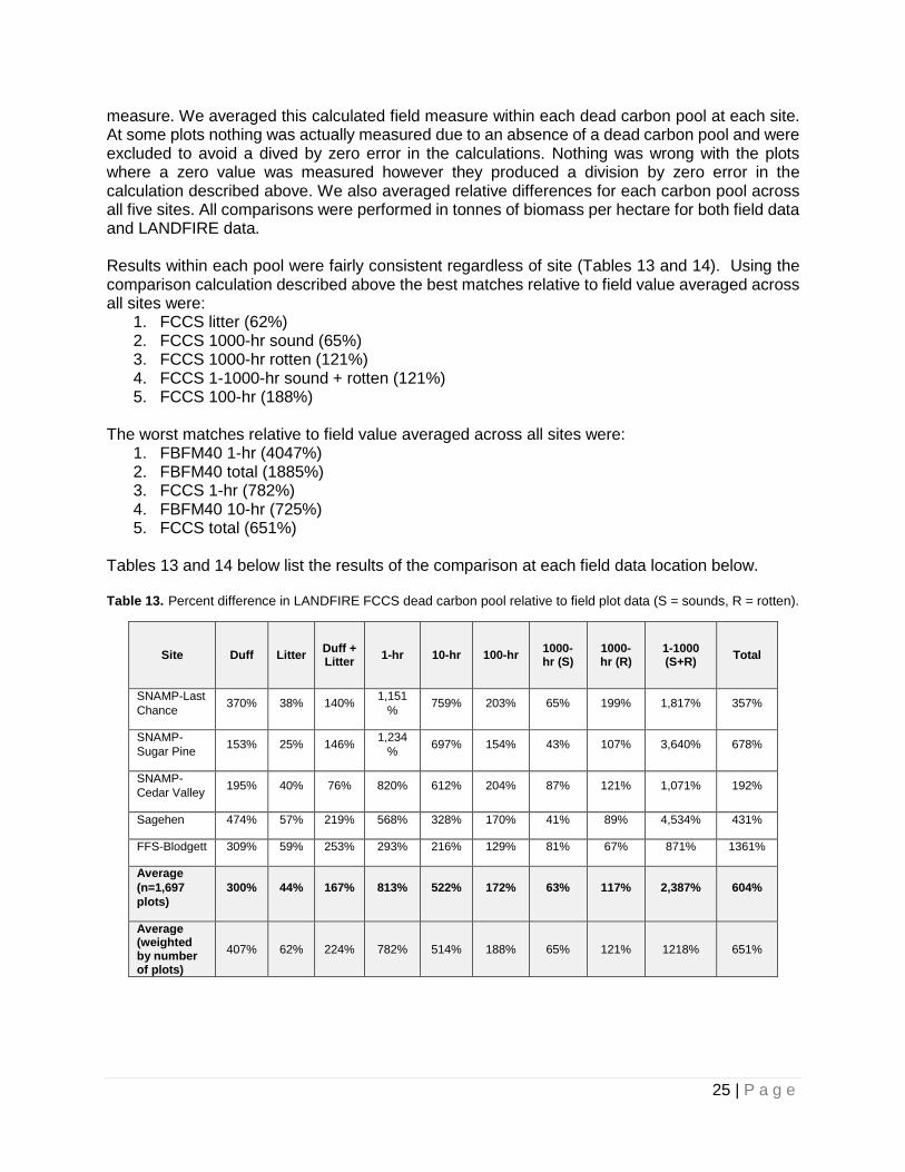
25 | P a g e
measure. We averaged this calculated field measure within each dead carbon pool at each site. At some plots nothing was actually measured due to an absence of a dead carbon pool and were excluded to avoid a dived by zero error in the calculations. Nothing was wrong with the plots where a zero value was measured however they produced a division by zero error in the calculation described above. We also averaged relative differences for each carbon pool across all five sites. All comparisons were performed in tonnes of biomass per hectare for both field data and LANDFIRE data. Results within each pool were fairly consistent regardless of site (Tables 13 and 14). Using the comparison calculation described above the best matches relative to field value averaged across all sites were:
1. FCCS litter (62%) 2. FCCS 1000-hr sound (65%) 3. FCCS 1000-hr rotten (121%) 4. FCCS 1-1000-hr sound + rotten (121%) 5. FCCS 100-hr (188%)
The worst matches relative to field value averaged across all sites were:
1. FBFM40 1-hr (4047%) 2. FBFM40 total (1885%) 3. FCCS 1-hr (782%) 4. FBFM40 10-hr (725%) 5. FCCS total (651%)
Tables 13 and 14 below list the results of the comparison at each field data location below. Table 13. Percent difference in LANDFIRE FCCS dead carbon pool relative to field plot data (S = sounds, R = rotten).
Site Duff Litter Duff + Litter
1-hr 10-hr 100-hr 1000-hr (S)
1000-hr (R)
1-1000 (S+R)
Total
SNAMP-Last
Chance 370% 38% 140%
1,151
% 759% 203% 65% 199% 1,817% 357%
SNAMP-
Sugar Pine 153% 25% 146%
1,234
% 697% 154% 43% 107% 3,640% 678%
SNAMP-
Cedar Valley 195% 40% 76% 820% 612% 204% 87% 121% 1,071% 192%
Sagehen 474% 57% 219% 568% 328% 170% 41% 89% 4,534% 431%
FFS-Blodgett 309% 59% 253% 293% 216% 129% 81% 67% 871% 1361%
Average
(n=1,697
plots)
300% 44% 167% 813% 522% 172% 63% 117% 2,387% 604%
Average (weighted by number of plots)
407% 62% 224% 782% 514% 188% 65% 121% 1218% 651%
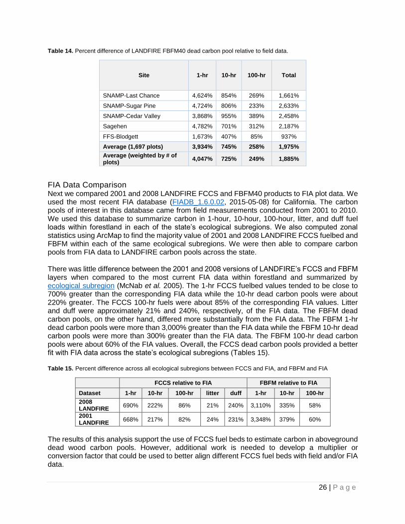
26 | P a g e
Table 14. Percent difference of LANDFIRE FBFM40 dead carbon pool relative to field data.
Site 1-hr 10-hr 100-hr Total
SNAMP-Last Chance 4,624% 854% 269% 1,661%
SNAMP-Sugar Pine 4,724% 806% 233% 2,633%
SNAMP-Cedar Valley 3,868% 955% 389% 2,458%
Sagehen 4,782% 701% 312% 2,187%
FFS-Blodgett 1,673% 407% 85% 937%
Average (1,697 plots) 3,934% 745% 258% 1,975%
Average (weighted by # of plots)
4,047% 725% 249% 1,885%
FIA Data Comparison Next we compared 2001 and 2008 LANDFIRE FCCS and FBFM40 products to FIA plot data. We used the most recent FIA database (FIADB_1.6.0.02, 2015-05-08) for California. The carbon pools of interest in this database came from field measurements conducted from 2001 to 2010. We used this database to summarize carbon in 1-hour, 10-hour, 100-hour, litter, and duff fuel loads within forestland in each of the state’s ecological subregions. We also computed zonal statistics using ArcMap to find the majority value of 2001 and 2008 LANDFIRE FCCS fuelbed and FBFM within each of the same ecological subregions. We were then able to compare carbon pools from FIA data to LANDFIRE carbon pools across the state. There was little difference between the 2001 and 2008 versions of LANDFIRE’s FCCS and FBFM layers when compared to the most current FIA data within forestland and summarized by ecological subregion (McNab et al. 2005). The 1-hr FCCS fuelbed values tended to be close to 700% greater than the corresponding FIA data while the 10-hr dead carbon pools were about 220% greater. The FCCS 100-hr fuels were about 85% of the corresponding FIA values. Litter and duff were approximately 21% and 240%, respectively, of the FIA data. The FBFM dead carbon pools, on the other hand, differed more substantially from the FIA data. The FBFM 1-hr dead carbon pools were more than 3,000% greater than the FIA data while the FBFM 10-hr dead carbon pools were more than 300% greater than the FIA data. The FBFM 100-hr dead carbon pools were about 60% of the FIA values. Overall, the FCCS dead carbon pools provided a better fit with FIA data across the state’s ecological subregions (Tables 15). Table 15. Percent difference across all ecological subregions between FCCS and FIA, and FBFM and FIA
FCCS relative to FIA FBFM relative to FIA
Dataset 1-hr 10-hr 100-hr litter duff 1-hr 10-hr 100-hr
2008 LANDFIRE
690% 222% 86% 21% 240% 3,110% 335% 58%
2001 LANDFIRE
668% 217% 82% 24% 231% 3,348% 379% 60%
The results of this analysis support the use of FCCS fuel beds to estimate carbon in aboveground dead wood carbon pools. However, additional work is needed to develop a multiplier or conversion factor that could be used to better align different FCCS fuel beds with field and/or FIA data.

27 | P a g e
28 | P a g e
Step 6: Identify Carbon Considerations of Forest Management and Harvested Wood Products Quantifying carbon stock changes associated with direct human-induced ‘degradation’ of forests and ‘devegetation’ of other vegetation types is complicated by variations in the intensity of activities such as timber harvesting (including both commercial and non-commercial operations) according to ownership type. Vegetation management and harvest activities lead to carbon stock changes that are difficult to quantify using remotely-sensed data since such activities are periodic in nature and harvested carbon stocks can recover at varying rates in between data acquisition years. Assessing stock changes from vegetation management and harvest activities requires calibration between site-level removal (harvest) data and remotely-sensed data that is adjusted for land ownership type and the temporal lag of monitoring data. Moreover, removed forest biomass should not be accounted for as an immediate emission since a fraction will be sequestered in wood products over a variable lifetime. In response to this challenge, we developed: 1) methodologies that use existing datasets to allocate areas with harvest activities, and categorize these harvest activities to the largest extend possible with biomass removal intensities, and 2) a crosswalk from defined harvest activities towards 100-year lifecycle emissions (losses) associated with these harvest activities and the wood products derived from these activities.
Harvest Operations in California We applied the LANDFIRE “Disturbance” 1999-2012 data layer to California state boundaries and
filtered for all harvest related disturbance types, namely ‘Clearcut’, ‘Thinning’, and ‘Harvest’ (Table
16). The following paragraph describes the data layer (LANDFIRE 2016) as:
LANDFIRE disturbance data are developed to provide temporal and spatial information
related to landscape change for determining vegetation transitions over time and for
making subsequent updates to LANDFIRE vegetation, fuel and other data. Disturbance
data include attributes associated with disturbance year, type, and severity. These data
are developed through use of Landsat satellite imagery, local agency derived disturbance
polygons, and other ancillary data. From the abstract: The disturbance data are developed
through a multistep process. Inputs to this process include; Landsat imagery and derived
NBR (normalized burn ratio) data; polygon data developed by local agencies for the LF
Events geodatabase effort; fire data obtained from MTBS (Monitoring Trends in Burn
Severity), BARC (Burned Area Reflectance Classification), and RAVG (Rapid Assessment
of Vegetation Condition after Wildfire) fire mapping efforts, PAD (Protected Area
Database) data, and Smartfire ignition point buffer polygons (buffer distance dependent
on sensor accuracy). LANDSAT imagery and derived NBR data are not included in Alaska
disturbance grid development. LF Event polygon data are provided to LANDFIRE by
various local, regional, and national agencies and organizations. Disturbance type and
year information is included as attributes for each polygon and transferred to the
disturbance grids. Severity is determined by using dNBR (difference Normalized Burn
Ratio) data classified into high, medium, and low severity levels based on dNBR standard
deviation thresholds. Vegetation Change Tracker (VCT) algorithms (Huang, et. al. 2008)
were used to identify disturbances outside of LF Events for the LF2008 effort (years 1999-
2008). Multi-Index Integrated Change Algorithm (MIICA) methods (Jin, et. al. 2013) were
used to identify additional change in 2008 as well as disturbances in 2009 and 2010 for
the LF2010 effort. Since disturbance type (i.e. causality) is not determined in the VCT or
MIICA processes, a spatial analysis is done comparing the output to buffered (500 meter)

29 | P a g e
LF Events, Protected Area Database GAP Status information (land use and management
characteristics), and Smartfire ignition point buffer polygons. While not providing a precise
type of disturbance, this analysis provides information useful for narrowing down the types
of disturbance that could or could not typically occur. Each zone has 13 disturbance grids,
one for each year 1999 to 2012. Each grid is attributed with year, disturbance type (if
known, otherwise a description of possible types), severity, data sources, and confidence
(type and severity). VdistYEAR grids are a composite of the last ten years of disturbance
grids recoded by disturbance type, disturbance severity, and time since disturbance YEAR
to meet LANDFIRE vegetation transition modeling needs. Fire occurrences take
precedence, followed by the most recent disturbance taking precedence.
Table 16. Harvest-related disturbance types in LANDFIRE Disturbance 1999-2012 dataset (Source: LANDFIRE 2015).
Attribute Enumerated
Value Enumerated Value Description
Dist_Type Clearcut The cutting of essentially all trees, producing a fully exposed microclimate for the development of a new age class.
Dist_Type Harvest
A general term for the cutting, felling, and gathering of forest timber. The term harvest was assigned to events where there was not enough information available to call them one of the 2 distinct types, clearcut or thinning.
Dist_Type Thinning
A tree removal practice that reduces tree density and competition between trees in a stand. Thinning concentrates growth on fewer, high-quality trees, provides periodic income, and generally enhances tree vigor.
Wood Products Carbon Assessment We identified the percentage of merchantable timber volume from the total study area landscape
(i.e., California) to estimate carbon loss for a given harvest activity (i.e., each for “clearcut”,
“harvest”, and “thinning” from Table 16 above). Using measured data from 28 harvest sites (partial
and clearcut) covering a total of 2,781 ha (Stewart and Nakamura 2012), and we generated
average carbon loss from each harvest activity type, as well as multipliers on carbon stored in
logs for different harvest operations on private timberlands (Table 17).
Table 17. Landscape carbon loss and merchantable volumes on private (Stewart and Nakamura 2012) and public
(Saah et al. 2012) land.
Ownership Type
Harvest Type
Mean Total Harvest Carbon
Density (MgC/ha)
Mean Merchantable
Carbon Density (MgC/ha)
Percent Merchantable
of Total Harvest Carbon
Density
Private Clearcut 48.9 43.4 89%
Public Clearcut 48.9 43.4 89%
Private Partial cut 21.0 7.3 42%
Public Partial cut 11.8 6.9 42%
Private Harvest N/A N/A 72%
Public Harvest N/A N/A 44%
30 | P a g e
For carbon loss (emissions) and harvest carbon density estimates on public lands, we compared timberland carbon densities for mature forest stands on public and private ownerships across California using Forest Inventory Analysis data (FIA 2015) for the time period of interest (1999 to 2012). We detected no discernable difference in carbon density (MgC/ha) and therefore assumed the same carbon stocking (48.9 MgC/ha) and wood product carbon density (43.4 MgC/ha) from public timberlands as from private timberlands.2 For thinning/partial cuts on public lands, we used estimates of 6.9 MgC/ha in merchantable carbon densities (Saah et al. 2012) and assumed a similar ratio in merchantable vs. total harvest carbon density as for private lands. To convert MgC to million board foot (mmbf), we used a conversion rate of 572 MgC/mmbf (Skog and Nicholson 2000). For the LANDFIRE disturbance “harvest” category, which enumerates all harvest sites that could
not be allocated to either thinning/partial cut or clearcut activities, we calculated a merchantable
vs. total harvest volume ratio based on the normalized total harvest volumes reported for
LANDFIRE disturbance categories for “thinning” and “clearcut” and multiplied by the respective
ratio of merchantable volumes for each of these two categories.3
Next, we generated carbon loss multipliers over a 100 year timeframe for those harvest volumes. Since wood products will store carbon in-use and post-use when landfilled the fraction of carbon stored in these wood products over a given timespan needs to be subtracted from landscape carbon loss. Using numbers from Smith et al. (2006), which are the basis for the national 1605(B) Voluntary
Reporting of Greenhouse Gases Program lookup tables as well as estimates from the University
of California (2015)4 Carbon Sequestration Tool for THPs, we estimated that 36% or 46% of C,
respectively, would be permanently stored in wood products over a 100 year time frame under a
normal California wood products life span. Carbon not used in wood products (unrecovered
residues, forest and sawmill residues used for bioenergy, etc.) was assumed to be emitted
completely over this timeframe.
Validation Validation of LANDFIRE outcomes were based on: 1) harvested acreage on private timberlands
as reported by CALFIRE (2010), 2) carbon stock loss estimates on a per acre basis by harvest
type using various other references (Table 17), as well as 3) reported merchantable volume
estimates as reported by the California State Board of Equalization (BOE 2015, Table 18). Using
this data, the BOE Timber Yield Tax program sets the harvest value of timber and collects an in
lieu tax when it is harvested. Not all carbon loss associated with harvest activities in the first as
well as last year of the time period of interest 2001 to 2010 were captured by the LANDFIRE
dataset due to continuous data collection efforts. We therefore included only 50% of the BOE
reported harvest volumes for the first (2001) and last (2010) year.
Landscape Harvest Impact 2001-2010 There is no spatially explicit dataset available to validate acreage outcomes from the LANDFIRE
Disturbance layer except for CALFIRE data on harvests from private lands from 2001 to 2008
(CALFIRE 2010) totaling 395,611 ha. Prorating this acreage to 2010 results in a total acreage
2 See ‘Wood product C pools from CA 1999-2012 2015-10-16.xls’; sheet ‘FIA owner C density’. 3 See ‘Disturbance_2001_2010 2015-11-16.xls’; sheet ‘Dashboard’; cell B28/C28. 4 Numbers for mixed conifer stands, see also ‘Wood product C pools from CA 1999-2012 2015-10-16.xls’; sheet ‘Dashboard’, cell J8.
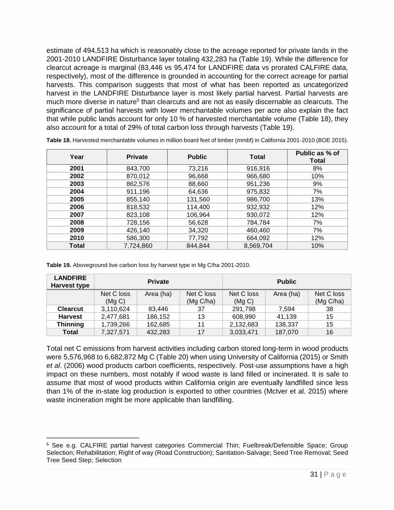
31 | P a g e
estimate of 494,513 ha which is reasonably close to the acreage reported for private lands in the
2001-2010 LANDFIRE Disturbance layer totaling 432,283 ha (Table 19). While the difference for
clearcut acreage is marginal (83,446 vs 95,474 for LANDFIRE data vs prorated CALFIRE data,
respectively), most of the difference is grounded in accounting for the correct acreage for partial
harvests. This comparison suggests that most of what has been reported as uncategorized
harvest in the LANDFIRE Disturbance layer is most likely partial harvest. Partial harvests are
much more diverse in nature5 than clearcuts and are not as easily discernable as clearcuts. The
significance of partial harvests with lower merchantable volumes per acre also explain the fact
that while public lands account for only 10 % of harvested merchantable volume (Table 18), they
also account for a total of 29% of total carbon loss through harvests (Table 19).
Table 18. Harvested merchantable volumes in million board feet of timber (mmbf) in California 2001-2010 (BOE 2015).
Year Private Public Total Public as % of
Total
2001 843,700 73,216 916,916 8%
2002 870,012 96,668 966,680 10%
2003 862,576 88,660 951,236 9%
2004 911,196 64,636 975,832 7%
2005 855,140 131,560 986,700 13%
2006 818,532 114,400 932,932 12%
2007 823,108 106,964 930,072 12%
2008 728,156 56,628 784,784 7%
2009 426,140 34,320 460,460 7%
2010 586,300 77,792 664,092 12%
Total 7,724,860 844,844 8,569,704 10%
Table 19. Aboveground live carbon loss by harvest type in Mg C/ha 2001-2010.
LANDFIRE Harvest type
Private Public
Net C loss (Mg C)
Area (ha) Net C loss (Mg C/ha)
Net C loss (Mg C)
Area (ha) Net C loss (Mg C/ha)
Clearcut 3,110,624 83,446 37 291,798 7,594 38
Harvest 2,477,681 186,152 13 608,990 41,139 15
Thinning 1,739,266 162,685 11 2,132,683 138,337 15
Total 7,327,571 432,283 17 3,033,471 187,070 16
Total net C emissions from harvest activities including carbon stored long-term in wood products
were 5,576,968 to 6,682,872 Mg C (Table 20) when using University of California (2015) or Smith
et al. (2006) wood products carbon coefficients, respectively. Post-use assumptions have a high
impact on these numbers, most notably if wood waste is land filled or incinerated. It is safe to
assume that most of wood products within California origin are eventually landfilled since less
than 1% of the in-state log production is exported to other countries (McIver et al. 2015) where
waste incineration might be more applicable than landfilling.
5 See e.g. CALFIRE partial harvest categories Commercial Thin; Fuelbreak/Defensible Space; Group Selection; Rehabilitation; Right of way (Road Construction); Sanitation-Salvage; Seed Tree Removal; Seed Tree Seed Step; Selection
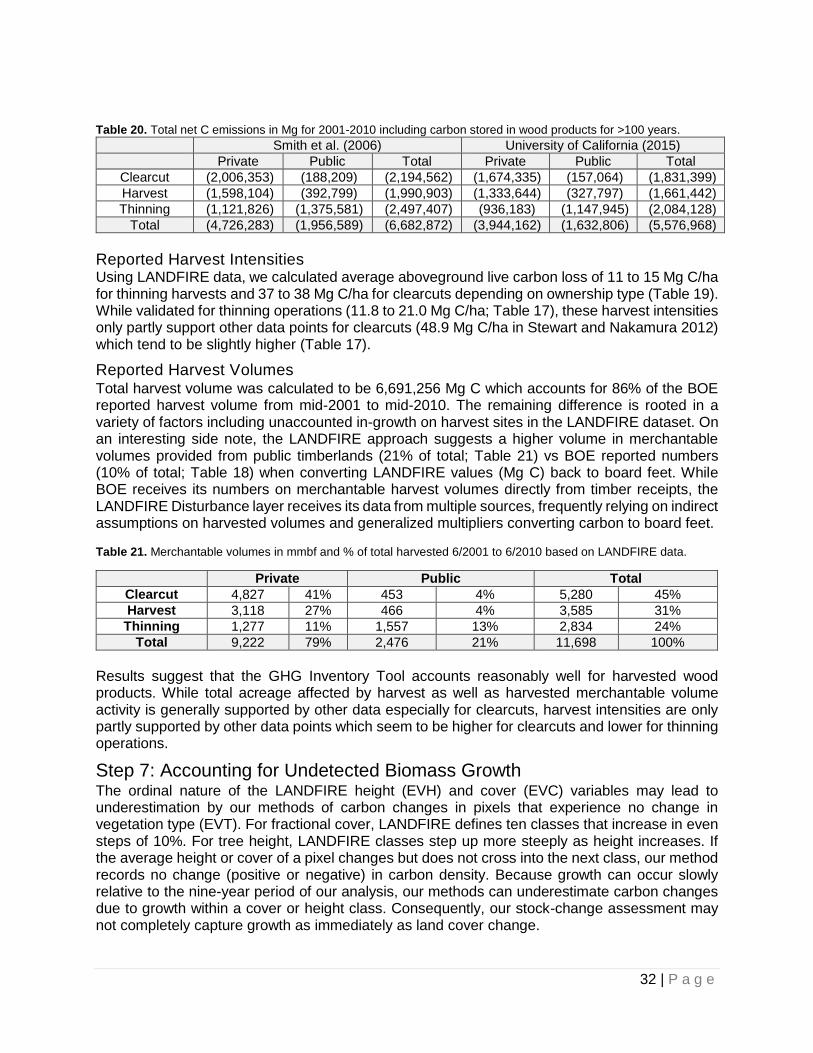
32 | P a g e
Table 20. Total net C emissions in Mg for 2001-2010 including carbon stored in wood products for >100 years.
Smith et al. (2006) University of California (2015)
Private Public Total Private Public Total
Clearcut (2,006,353) (188,209) (2,194,562) (1,674,335) (157,064) (1,831,399)
Harvest (1,598,104) (392,799) (1,990,903) (1,333,644) (327,797) (1,661,442)
Thinning (1,121,826) (1,375,581) (2,497,407) (936,183) (1,147,945) (2,084,128)
Total (4,726,283) (1,956,589) (6,682,872) (3,944,162) (1,632,806) (5,576,968)
Reported Harvest Intensities Using LANDFIRE data, we calculated average aboveground live carbon loss of 11 to 15 Mg C/ha for thinning harvests and 37 to 38 Mg C/ha for clearcuts depending on ownership type (Table 19). While validated for thinning operations (11.8 to 21.0 Mg C/ha; Table 17), these harvest intensities only partly support other data points for clearcuts (48.9 Mg C/ha in Stewart and Nakamura 2012) which tend to be slightly higher (Table 17).
Reported Harvest Volumes Total harvest volume was calculated to be 6,691,256 Mg C which accounts for 86% of the BOE reported harvest volume from mid-2001 to mid-2010. The remaining difference is rooted in a variety of factors including unaccounted in-growth on harvest sites in the LANDFIRE dataset. On an interesting side note, the LANDFIRE approach suggests a higher volume in merchantable volumes provided from public timberlands (21% of total; Table 21) vs BOE reported numbers (10% of total; Table 18) when converting LANDFIRE values (Mg C) back to board feet. While BOE receives its numbers on merchantable harvest volumes directly from timber receipts, the LANDFIRE Disturbance layer receives its data from multiple sources, frequently relying on indirect assumptions on harvested volumes and generalized multipliers converting carbon to board feet. Table 21. Merchantable volumes in mmbf and % of total harvested 6/2001 to 6/2010 based on LANDFIRE data.
Private Public Total
Clearcut 4,827 41% 453 4% 5,280 45%
Harvest 3,118 27% 466 4% 3,585 31%
Thinning 1,277 11% 1,557 13% 2,834 24%
Total 9,222 79% 2,476 21% 11,698 100%
Results suggest that the GHG Inventory Tool accounts reasonably well for harvested wood products. While total acreage affected by harvest as well as harvested merchantable volume activity is generally supported by other data especially for clearcuts, harvest intensities are only partly supported by other data points which seem to be higher for clearcuts and lower for thinning operations.
Step 7: Accounting for Undetected Biomass Growth The ordinal nature of the LANDFIRE height (EVH) and cover (EVC) variables may lead to underestimation by our methods of carbon changes in pixels that experience no change in vegetation type (EVT). For fractional cover, LANDFIRE defines ten classes that increase in even steps of 10%. For tree height, LANDFIRE classes step up more steeply as height increases. If the average height or cover of a pixel changes but does not cross into the next class, our method records no change (positive or negative) in carbon density. Because growth can occur slowly relative to the nine-year period of our analysis, our methods can underestimate carbon changes due to growth within a cover or height class. Consequently, our stock-change assessment may not completely capture growth as immediately as land cover change.
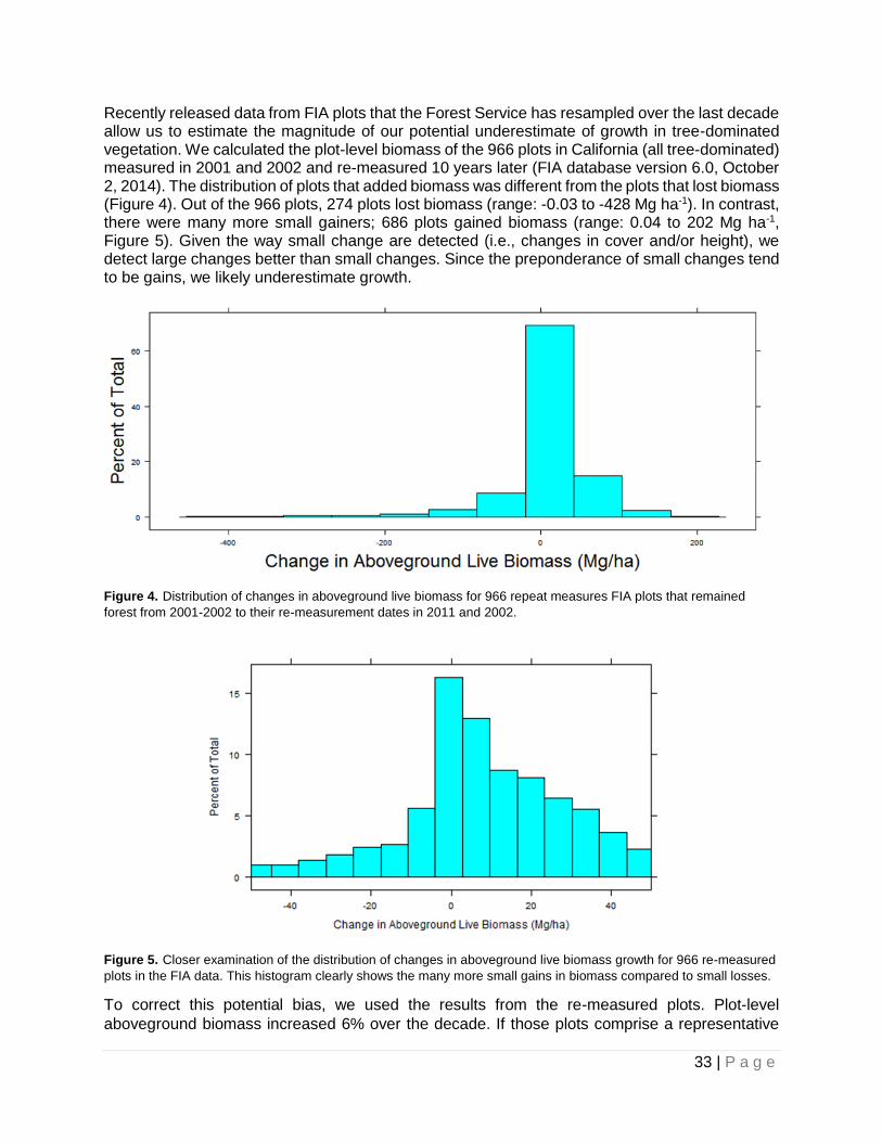
33 | P a g e
Recently released data from FIA plots that the Forest Service has resampled over the last decade allow us to estimate the magnitude of our potential underestimate of growth in tree-dominated vegetation. We calculated the plot-level biomass of the 966 plots in California (all tree-dominated) measured in 2001 and 2002 and re-measured 10 years later (FIA database version 6.0, October 2, 2014). The distribution of plots that added biomass was different from the plots that lost biomass (Figure 4). Out of the 966 plots, 274 plots lost biomass (range: -0.03 to -428 Mg ha-1). In contrast, there were many more small gainers; 686 plots gained biomass (range: 0.04 to 202 Mg ha-1, Figure 5). Given the way small change are detected (i.e., changes in cover and/or height), we detect large changes better than small changes. Since the preponderance of small changes tend to be gains, we likely underestimate growth.
Figure 4. Distribution of changes in aboveground live biomass for 966 repeat measures FIA plots that remained
forest from 2001-2002 to their re-measurement dates in 2011 and 2002.
Figure 5. Closer examination of the distribution of changes in aboveground live biomass growth for 966 re-measured
plots in the FIA data. This histogram clearly shows the many more small gains in biomass compared to small losses.
To correct this potential bias, we used the results from the re-measured plots. Plot-level
aboveground biomass increased 6% over the decade. If those plots comprise a representative
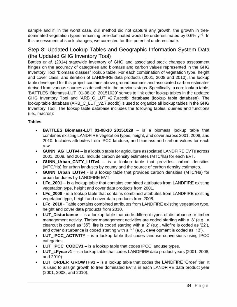
34 | P a g e
sample and if, in the worst case, our method did not capture any growth, the growth in tree-
dominated vegetation types remaining tree-dominated would be underestimated by 0.6% yr-1. In
this assessment of stock changes, we corrected for this potential underestimate.
Step 8: Updated Lookup Tables and Geographic Information System Data
(the Updated GHG Inventory Tool) Battles et al. (2014) statewide inventory of GHG and associated stock changes assessment
hinges on the accuracy of categories and biomass and carbon values represented in the GHG
Inventory Tool “biomass classes” lookup table. For each combination of vegetation type, height
and cover class, and iteration of LANDFIRE data products (2001, 2008 and 2010), the lookup
table developed for this project contains above ground biomass and associated carbon estimates
derived from various sources as described in the previous steps. Specifically, a core lookup table,
‘BATTLES_Biomass-LUT_01-08-10_20151029’ serves to link other lookup tables in the updated
GHG Inventory Tool and ‘ARB_C_LUT_v2.7.accdb’ database (lookup table database). The
lookup table database (ARB_C_LUT_v2.7.accdb) is used to organize all lookup tables in the GHG
Inventory Tool. The lookup table database includes the following tables, queries and functions
(i.e., macros):
Tables
BATTLES_Biomass-LUT_01-08-10_20151029 – is a biomass lookup table that
combines existing LANDFIRE vegetation types, height, and cover across 2001, 2008, and
2010. Includes attributes from IPCC landuse, and biomass and carbon values for each
row.
GUNN_AG_LUTv4 – is a lookup table for agriculture associated LANDFIRE EVTs across
2001, 2008, and 2010. Include carbon density estimates (MTC/ha) for each EVT.
GUNN_Urban_CNTY_LUTv4 – is a lookup table that provides carbon densities
(MTC/Ha) for urban landuses by county and the source of carbon density estimates.
GUNN_Urban_LUTv4 - is a lookup table that provides carbon densities (MTC/Ha) for
urban landuses by LANDFIRE EVT.
LFc_2001 – is a lookup table that contains combined attributes from LANDFIRE existing
vegetation type, height and cover data products from 2001.
LFc_2008 - is a lookup table that contains combined attributes from LANDFIRE existing
vegetation type, height and cover data products from 2008.
LFc_2010 - Table contains combined attributes from LANDFIRE existing vegetation type,
height and cover data products from 2010.
LUT_Disturbance – Is a lookup table that code different types of disturbance or timber
management activity. Timber management activities are coded starting with a ‘3’ (e.g., a
clearcut is coded as ‘35’), fire is coded starting with a ‘2’ (e.g., wildfire is coded as ‘22’),
and other disturbance is coded starting with a ‘1’ (e.g., development is coded as ‘13’).
LUT_IPCC_ACTIVITY – is a lookup table that codes landuse conversions using IPCC
categories.
LUT_IPCC_CODEV1 – is a lookup table that codes IPCC landuse types.
LUT_LFyearv1 – is a lookup table that codes LANDFIRE data product years (2001, 2008,
and 2010)
LUT_ORDER_GROWTHv1 – is a lookup table that codes the LANDFIRE ‘Order’ tier. It
is used to assign growth to tree dominated EVTs in each LANDFIRE data product year
(2001, 2008, and 2010).
35 | P a g e
Queries
IPCC_AC_CODE – this was originally a lookup that is now deprecated.
ARB_BIOMASS_LUT_v2.7 – is a lookup table that combine urban and agriculture carbon
densities with the BATTLES_Biomass-LUT_01-08-10_20151029
Macros
LUT_EXPORT – converts ‘ARB_C_LUT_v2.7.accdb’ access database tables and queries
into individual excel spreadsheets. These spreadsheets are used for geodatabases to
show distribution of biomass and carbon values across California and calculating carbon
stock change across LANDFIRE data product years. The following spreadsheets are
generated with this macro:
o LUT_ARB_BIOMASS_v2_7.xls
o LUT_GUNN_Urban_CNTYv4.xls
o LUT_IPCC_ACTIVITY.xls
o LUT_IPCC_CODEv1.xls
o LUT_LFYEARv1.xls
o LUT_LUT_Disturbance.xls
o LUT_ORDER_GROWTHv1.xls
The spreadsheets were then ingested into one to many different geodatabases through ArcGIS
model builder. The lookup tables are used for all carbon stock calculations. Geodatabases and
associated models for calculating stock changes are organized in the “02_Calculations” folder
using the same file structure as the LandCarbon Models used for conducting the calculations
contained in the ‘Toolbox.tbx’ file. Below is a brief description of each step where the model is
labeled in sequential order and their results are filed in a sub-directory using the same name:
01_Build_Biomass_LUT – model used to link IPCC Codes with the combined biomass
lookup table along with lookup table for growth to produce a master biomass lookup table.
02_Load_Landfire_Rasters – model procedures for loading biomass and carbon values
to raw combined (i.e., EVT, EVH, and EVC) LANDFIRE datasets.
03_Urban_County_MTCha – Model procedures used to combine county boundaries with
urban carbon values; creates a raster layer that contains mean carbon values for each
California county (ARB_URBAN_County_MTCha).
04_Calculate_Biomass_MTCha – model procedures for calculating carbon values by
cell and county for the study area. Combines values (total metric tonnes per hectare,
including adding in tree growth) for urban, agriculture and wildlands and creates multiple
raster files for each LANDFIRE product year in a geodatabase (B04_MAP_MTCha.gdb).
05_Calc_Total_Carbon – model convert carbon densities (MTC/ha) into total carbon
values (Metric tonnes of carbon), and summarizes values by different classifications of
interest including agriculture, urban, wildland, and IPCC landuse types. Produces per year
values.
06_Forest_Growth – model used to calculate carbon values associated with forest
growth across years. Adds growth coefficient (6%) to large tree category and generates a
raster showing where growth has occurred in the state.
07_Net_Carbon – model that calculates carbon values and rasters associated forest
growth to produce a net carbon estimate across years and the study area.
36 | P a g e
08_IPCC_CODE - model that calculates carbon values and rasters associated landuse
conversions across years and the study area. Carbon values (million metric tonnes of
carbon) associated with land conversions are captured in a spreadsheet
(IPCC_Summary_2010_2001.xlsx).
09_Load_Disturbance_Data – model used to generate disturbance codes and rasters
associated with different timber management activities for each year between 2001 and
2010.
10_Disturbance_Zone – combines rasters for each year and identifies the years with a
prioritized value associated with timber management. Also combine public and private
ownership attributes. Generates a raster attributed with priority timber management
activity. This analysis/model needs more investigation to flesh out how best to prioritize
management activities.
11_Disturbance_Stats – model used to run zonal statistics to combine all disturbances
into geodatabase. Attributes are used to summarize timber management and disturbances
(in acres) across years in a spreadsheet
(ARB_HARVEST_FIRE_ANNUAL_SUMMARY.xlsx).
The models should be run in sequence where the input data is pulled from the directory of the
previous model. This segmentation in the analytical process allows for the user to test individual
steps without having to recreate the entire simulation. This approach also allows for all the
intermediate products to be saved so they can potentially be used for additional analysis. Also
note that the models housed within the ArcGIS geodatabase (i.e., ‘Toolbox.tbx’) clearly illustrate
inputs, procedures and outputs for each model listed immediately above
A oral narrative that contains procedures for using the update GHG Inventory Tool along with a
description of all files and folders are also captured in a webinar recording titled “2015-11-19
10.22 ARB Accounting Update.mp4” and is included as a deliverable for this project.
Step 9: Conduct Carbon Stock Change Evaluation Information and products (e.g., databases, spreadsheets and GIS data) generated through Steps
1 through 8 describe the procedures for organizing data and information for calculating estimates
of above ground carbon stock change in California for a given LANDFIRE product year (2001,
2008, and 2010). Using the updated GHG Inventory Tool (in step 8), total above ground live
carbon was preliminarily estimated to be about 2,696 MMTC in 2001, and 2551 MMTC in 2010,
representing an overall loss of about -145 MMTC over the time period (Table 22) or a loss of
approximately -16.1 MMTC yr-1. The greatest estimated loss in carbon pools converting to
grasslands with wetlands remaining relatively unchanged across 2001 and 2010 (Table 22).
These estimates include above ground live biomass associated with forestlands, croplands,
grasslands, wetlands, settlements, and other lands. However, it is important to note that these
estimates are preliminary and should not be formally or informally reported. The estimates have
not been adjusted for biomass burning, wildfire emissions, or harvested wood products.
Forestlands represent the largest carbon pool within the study area, storing about 11 times more
carbon than other land categories combined. These adjustments have been incorporated or
addressed as separate elements.
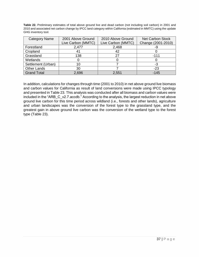
37 | P a g e
Table 22. Preliminary estimates of total above ground live and dead carbon (not including soil carbon) in 2001 and
2010 and associated net carbon change by IPCC land category within California (estimated in MMTC) using the update
GHG inventory tool.
Category Name 2001 Above Ground Live Carbon (MMTC)
2010 Above Ground Live Carbon (MMTC)
Net Carbon Stock Change (2001-2010)
Forestland 2,477 2,468 -9
Cropland 41 42 0
Grassland 138 27 -111
Wetlands 0 0 0
Settlement (Urban) 10 7 -3
Other Lands 30 7 -23
Grand Total 2,696 2,551 -145
In addition, calculations for changes through time (2001 to 2010) in net above ground live biomass
and carbon values for California as result of land conversions were made using IPCC typology
and presented in Table 23. This analysis was conducted after all biomass and carbon values were
included in the “ARB_C_v2.7.accdb.” According to the analysis, the largest reduction in net above
ground live carbon for this time period across wildland (i.e., forests and other lands), agriculture
and urban landscapes was the conversion of the forest type to the grassland type, and the
greatest gain in above ground live carbon was the conversion of the wetland type to the forest
type (Table 23).
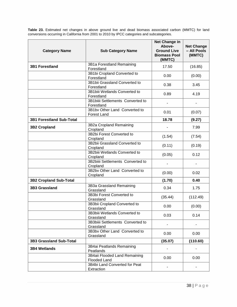
38 | P a g e
Table 23. Estimated net changes in above ground live and dead biomass associated carbon (MMTC) for land
conversions occurring in California from 2001 to 2010 by IPCC categories and subcategories.
Category Name Sub Category Name
Net Change in Above-
Ground Live Biomass Pool
(MMTC)
Net Change – All Pools
(MMTC)
3B1 Forestland 3B1a Forestland Remaining Forestland
17.50 (16.85)
3B1bi Cropland Converted to Forestland
0.00 (0.00)
3B1bii Grassland Converted to Forestland
0.38 3.45
3B1biii Wetlands Converted to Forestland
0.89 4.19
3B1biiii Settlements Converted to Forestland
- -
3B1bv Other Land Converted to Forest Land
0.01 (0.07)
3B1 Forestland Sub-Total 18.78 (9.27)
3B2 Cropland 3B2a Cropland Remaining Cropland
- 7.99
3B2bi Forest Converted to Cropland
(1.54) (7.54)
3B2bii Grassland Converted to Cropland
(0.11) (0.19)
3B2biii Wetlands Converted to Cropland
(0.05) 0.12
3B2biiii Settlements Converted to Cropland
- -
3B2bv Other Land Converted to Cropland
(0.00) 0.02
3B2 Cropland Sub-Total (1.70) 0.40
3B3 Grassland 3B3a Grassland Remaining Grassland
0.34 1.75
3B3bi Forest Converted to Grassland
(35.44) (112.49)
3B3bii Cropland Converted to Grassland
0.00 (0.00)
3B3biii Wetlands Converted to Grassland
0.03 0.14
3B3biiii Settlements Converted to Grassland
- -
3B3bv Other Land Converted to Grassland
0.00 0.00
3B3 Grassland Sub-Total (35.07) (110.60)
3B4 Wetlands 3B4ai Peatlands Remaining Peatlands
- -
3B4aii Flooded Land Remaining Flooded Land
0.00 0.00
3B4bi Land Converted for Peat Extraction
- -
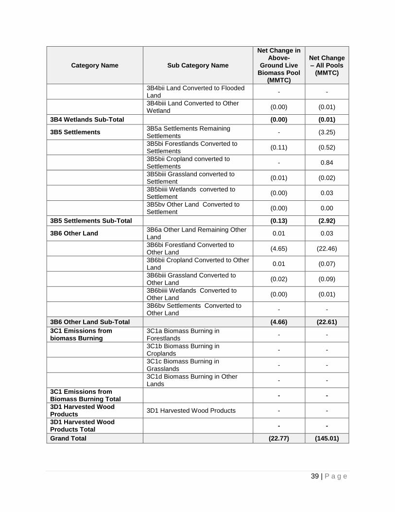
39 | P a g e
Category Name Sub Category Name
Net Change in Above-
Ground Live Biomass Pool
(MMTC)
Net Change – All Pools
(MMTC)
3B4bii Land Converted to Flooded Land
- -
3B4biii Land Converted to Other Wetland
(0.00) (0.01)
3B4 Wetlands Sub-Total (0.00) (0.01)
3B5 Settlements 3B5a Settlements Remaining Settlements
- (3.25)
3B5bi Forestlands Converted to Settlements
(0.11) (0.52)
3B5bii Cropland converted to Settlements
- 0.84
3B5biii Grassland converted to Settlement
(0.01) (0.02)
3B5biiii Wetlands converted to Settlement
(0.00) 0.03
3B5bv Other Land Converted to Settlement
(0.00) 0.00
3B5 Settlements Sub-Total (0.13) (2.92)
3B6 Other Land 3B6a Other Land Remaining Other Land
0.01 0.03
3B6bi Forestland Converted to Other Land
(4.65) (22.46)
3B6bii Cropland Converted to Other Land
0.01 (0.07)
3B6biii Grassland Converted to Other Land
(0.02) (0.09)
3B6biiii Wetlands Converted to Other Land
(0.00) (0.01)
3B6bv Settlements Converted to Other Land
- -
3B6 Other Land Sub-Total (4.66) (22.61)
3C1 Emissions from biomass Burning
3C1a Biomass Burning in Forestlands
- -
3C1b Biomass Burning in Croplands
- -
3C1c Biomass Burning in Grasslands
- -
3C1d Biomass Burning in Other Lands
- -
3C1 Emissions from Biomass Burning Total
- -
3D1 Harvested Wood Products
3D1 Harvested Wood Products - -
3D1 Harvested Wood Products Total
- -
Grand Total (22.77) (145.01)
40 | P a g e
CONCLUSIONS, RECOMMENDATIONS AND NEXT STEPS Managing Typology Changes in LANDFIRE Existing Vegetation Types. LANDFIRE is an evolving product that is expanding its capacity in resource management beyond wildfires. It is co-funded by two federal agencies (US Department of Agriculture and US Department of the Interior). Thus it has many constituents. In each revision, it tries to respond to requests for a variety of improvements. Also a founding principle in regard to its vegetation mapping was to abide by guidelines in the National Vegetation Classification System. In some respects, LANDFIRE has become the national vegetation map by default. However, as a consequence, continual modification of EVT’s is likely as constituent needs and standards change. For the updated carbon stock assessment tool, our biomass classes are based on the 2008 EVT’s. As noted, the trend is to produce more finely resolved vegetation classes and LANDFIRE is committed to a hierarchical approach. The new EVT’s will fit under the coarser 2008 classes making it possible to create cross-walks that maintain the consistency of the carbon accounting over time. The refinements in the 2010 EVT’s do suggest the potential for more precise carbon estimation. For the blue oak woodland case study, divisions based on vegetation structure were more relevant for carbon estimation than ones based on species composition. Certainly dividing EVT’s that cross physiognomic gradients (e.g., woodland/savanna or woodland/shrubland) into more structurally consistent classes would also reflect gradients in carbon storage. However, we found that even the more cohesive units contained a great deal of plot-to-plot variation in above-ground live biomass. Moreover, results from the vegetation mapping assessment of LANDFIRE (NatureServe 2012) document the challenge in differentiating discrete groups when the vegetation itself is very heterogeneous. In short, LANDFIRE can assign coarser scale vegetation classes with much greater accuracy. Given that the major source of uncertainty in the statewide carbon assessment was LANDFIRE classification (Battles et al. 2014), we recommend against recalculating biomass classes for the refined EVT’s. In fact, our evaluation suggests that we could gain consistency and reduce uncertainty without a major fall-off in precision by estimating carbon stores at as function of LANDFIRE subclass (e.g., closed-canopy, evergreen forest, sparse canopy mixed forests, open canopy deciduous forest). These more coarse-scale designations are more reliably determined by LANDFIRE and could be segregated by major ecological regions in California to parse major carbon density gradients. For example, the closed-canopy evergreen forest in the north coast supersection would be one group and the closed-canopy evergreen forest in the Sierra Nevada another. Logistically, it would make the most sense to consider this alternative approach the next time new biomass classes are introduced by the LANDFIRE program. Dead Wood Carbon Pools. LANDFIRE’s 100-hr fuels, whether a component of a FBFM or a fuelbed, were most consistently close to field-measured values of all the dead carbon pools. The current comparison only included mixed conifer forest plots in the Sierra Nevada. Field data from other forest types and other regions of California are needed. Additionally, all the datasets are best matched with the 2008 version of LANDFIRE. Several FCCS fuelbeds and FBFMs dominate the LANDFIRE mapping at these sites and have an outsized influence on the comparison, including:
FCCS o 37 Ponderosa pine-Jeffrey pine forest o 17 Red fir forest
41 | P a g e
o 627 Modified or Managed Xeric Understory 2 (based on FBFM TU5 , “very high load, dry climate timber-shrub”)
o 7 Douglas-fir-Sugar pine-Tan oak forest
FBFM40 values o 165/TU5 (“very high load, dry climate timber-shrub”) and 186/TL6 (“moderate load
broadleaf litter”) Above Ground Carbon Stock Changes Analysis (2001 to 2010). The carbon stock change estimates represented in this report are the result of testing different elements (e.g., tables, models) of the updated GHG Inventory Tool. Consequently, the estimates should be considered preliminary and should not be represented as an official or qualified accounting of above ground carbon stock change for the state as additional refinement of assumptions and inputs are needed to be informed by ARB staff as appropriate. Next Steps. The following next steps were identified for additionally refining the GHG Inventory Tool and ARB’s effort to assess above ground carbon stock changes. Specifically, ARB may consider working toward the acquisition of annualized input/base data. Although LANDFIRE has been invaluable for providing good estimates of above ground biomass and associated carbon across the state for natural and working lands, LANDFIRE does not provide annual updates making regular assessment of carbon stocks not possible using this data source. Elements of annual updated vegetation and land cover data should also include improved data on:
1) wildfire emission and fuel beds, 2) tree mortality and rates of mortality (become an ever present issue associated with
drought conditions in California), 3) improved annual characterization of urban and agricultural biomass, 4) improved estimated of climate change induced type conversions – specifically
forest to shrub type conversions and 5) more frequent characterization of land cover changes and 6) improved forest structure characterization (e.g., tree height).
New data initiatives such as NASA’s Joint Emissivity Database Initiative (JEDI) could aid improved characterization of land cover characteristics on an annualized basis.
REFERENCES Allen-Diaz, Barbara; Bartolome, James W.; McClaran, Mitchel P. 1999. California oak savanna. In:
Anderson, Roger C.; Fralish, James S.; Baskin, Jerry M., eds. Savannas, barrens, and rock outcrop plant communities of North America. New York: Cambridge University Press: 322-339.
Bjorkman, J., J.H. Thorne, A. Hollander, N.E. Roth, R.M. Boynton, J. de Goede, Q. Xiao, K. Beardsley, G. McPherson, J.F. Quinn. March, 2015. Biomass, carbon sequestration and avoided emission: assessing the role of urban trees in California. Information Center for the Environment, University of California, Davis.
Boryan, C., Yang, Z., Mueller, R., Craig, M., 2011. Monitoring US agriculture: the US Department of Agriculture, National Agricultural Statistics Service, Cropland Data Layer Program. Geocarto International, 26(5), 341–358. http://nassgeodata.gmu.edu/CropScape/
California (CALFIRE) 2010. Chapter 1.2: Sustainable Working Forests and Rangelands. In: California's Forests and Rangelands: 2015 Assessment. CALFIRE's Fire and Resource Assessment Program (FRAP), Sacramento, CA, 34p.
California State Board of Equalization (BOE) 2015. California Timber Harvest Statistics. https://www.boe.ca.gov/proptaxes/pdf/harvyr2.pdf Last accessed: November 16 2015.
42 | P a g e
Carlisle, E., Smart, D., Williams, L.E., & Summers, M., 2010. California vineyard greenhouse gas emissions: Assessment of the available literature and determination of research needs. California Sustainable Wine Growing Alliance.
Ciais, P., C. Sabine, G. Bala, L. Bopp, V. Brovkin, J. Canadell, A. Chhabra, R. DeFries, J. Galloway, M. Heimann, C. Jones, C. Le Quéré, R.B. Myneni, S. Piao and P. Thornton, 2013: Carbon and Other Biogeochemical Cycles. In: Climate Change 2013: The Physical Science Basis. Contribution of Working Group I to the Fifth Assessment Report of the Intergovernmental Panel on Climate Change [Stocker, T.F., D. Qin, G.-K. Plattner, M. Tignor, S.K. Allen, J. Boschung, A. Nauels, Y. Xia, V. Bex and P.M. Midgley (eds.)]. Cambridge University Press, Cambridge, United Kingdom and New York, NY, USA.
Collins, B., S. Stephens, G. Roller, and J. Battles. 2011. Simulating fire and forest dynamics for a landscape fuel treatment project in the Sierra Nevada. Forest Science 57(2): 77-88.
DeJong, T. M., 2013. Developing a Carbon Budget, Physiology, Growth and Yield Model for Almond Trees. Almond Board of California. Final Report.
DOE 2007. Appendices to the Technical Guidelines: Part I Appendix: Forestry. Department of Energy, Washington DC, 280p. http://www.eia.doe.gov/oiaf/1605/Forestryappendix%5B1%5D.pdf. Last viewed on September 13 2012
FRAP 2010. Chapter 1.2Easter, Mark. 2015. Natural Resource Ecology Laboratory, Colorado State University. Personal communication.
Eve, M., D. Pape, M. Flugge, R. Steele, D. Man, M. Riley‐Gilbert, and S. Biggar, (Eds), 2014.
Quantifying Greenhouse Gas Fluxes in Agriculture and Forestry: Methods for Entity‐Scale Inventory. Technical Bulletin Number 1939. Office of the Chief Economist, U.S. Department of Agriculture, Washington, DC. July 2014.
FGDC. 2008. Federal Geographic Data Committee. National Vegetation Classification System. Version 2. FGDC-STD-005-2008 (Version 2).
Forest Inventory Analysis (FIA) 2015. EVALIDator Version 1.6.0.03. McCune, B., J.B. Grace, and D.L. Urban. 2002. Analysis of Ecological Communities. Gleneden Beach, OR: MjM Software Design.
IPCC 2013 McNab, W.H.; Cleland, D.T.; Freeouf, J.A.; Keys, Jr., J.E.; Nowacki, G.J.; Carpenter, C.A., comps. 2005.
Description of ecological subregions: sections of the conterminous United States [CD-ROM]. Washington, DC: U.S. Department of Agriculture, Forest Service. 80 p.
NatureServe. 2012. Expert Attribution for Auto-Key Improvements (LANDFIRE) and Advancing Methods for integration with the revised US-National Vegetation Classification Standard: GeoArea 3. Final Report: Boulder, CO.
NVCS. 2015. National Vegetation Classification Standard. https://www.fgdc.gov/standards/projects/FGDC-standards-projects/vegetation.
http://apps.fs.fed.us/Evalidator/evalidator.jsp Last accessed: November 16 2015. LANDFIRE 2015. Disturbance 1999-2012, Fuel Disturbance, Vegetation Disturbance.
http://www.landfire.gov/disturbance_2.php Last accessed: November 16 2015. LANDFIRE 2016. LANDFIRE Data Dictionary.
http://www.landfire.gov/DataDictionary/lf_vdist2012.xml Last accessed: January 3 2016. Li, S., Potter, C., & Hiatt, C., 2012. Monitoring of net primary production in California rangelands
using Landsat and MODIS satellite remote sensing. Scientific Research, Natural Resources, Vol. 3, 56-65. DOI: 10.4236/nr.2012.32009.
McGroddy, M.E., T. Daufresne, and L.O. Hedin. 2004. Scaling of C:N:P stoichiometry in forests worldwide: Implications of terrestrial Redfield-type ratios. Ecology 85: 2390-2401.
McIver, CP, Meek, JP, Scudder, MG, Sorenson, CB, Morgan, TA, Christensen, GA, 2015. DRAFT - In Production California’s Forest Products Industry and Timber Harvest, 2012. PNW-GTR-908. USDA Forest Service, Pacific Northwest Research Station, 53p.
43 | P a g e
Mitchell, J., Hartz, T., Pettygrove, S., Munk, D., May, D., Menezes, F., Diener, J., & O'Neill, T. 1999. Organic matter recycling varies with crops grown. California Agriculture, 53(4), 37-40.
Morgan, K. T., Scholberg, J. M. S., Obreza, T. A., & Wheaton, T. A. 2006. Size, biomass, and nitrogen relationships with sweet orange tree growth. Journal of the American Society for Horticultural Science, 131(1), 149-156.
Murphy, William J., 1994. University of Missouri Extension, Department of Agronomy, G4020, Tables for Weights and Measurements: Crops. Publication: #G4020. http://extension.missouri.edu/publications/DisplayPub.aspx?P=G4020
National Agricultural Statistics Service. http://quickstats.nass.usda.gov/ Ottmar, R.D.; Sandberg, D.V.; Riccardi, C.L.; Prichard, S.J. 2007. An overview of the fuel
characteristic classification system – quantifying, classifying, and creating fuelbeds for resource planning. Canadian Journal of Forest Research. 37(12): 2383-2393.
Penman, J., et. al 2003. Intergovernmental Panel on Climate Change (IPCC). Good practice guidance for land use, land-use change and forestry. Institute for Global Environmental Strategies. http://www.ipcc-nggip.iges.or.jp/public/gpglulucf/gpglulucf_contents.html.
Prichard, S. J., Sandberg, D. V., Ottmar, R. D., Eberhardt, E., Andreu, A., Eagle, P., Swedin, K.. 2013. Fuel Characteristic Classification System version 3.0: technical documentation. Gen. Tech. Rep. PNW-GTR-887. Portland, OR: U.S. Department of Agriculture, Forest Service, Pacific Northwest Research Station. 79 p. http://www.fs.fed.us/pnw/pubs/pnw_gtr887.pdf.
Putnam, Daniel H. 2015. Alfalfa and Foreage News. UC Cooperative Extension: http://ucanr.edu/blogs/blogcore/postdetail.cfm?postnum=17721
Rosecrance, R. and Lovatt, C. 2003. Seasonal Patterns of Nutrient Uptake and Partitioning as a Function of Crop Load of the 'Hass' avocado. CSU, Chico. Final Report.
Ruesch, Aaron, and Holly K. Gibbs. 2008. New IPCC Tier-1 Global Biomass Carbon Map for the Year 2000. Carbon Dioxide Information Analysis Center [http://cdiac.ornl.gov], Oak Ridge National Laboratory, Oak Ridge, Tennessee. http://cdiac.ornl.gov/epubs/ndp/global_carbon/carbon_documentation.html
Ryals, R., & Silver, W. L. 2013. Effects of organic matter amendments on net primary productivity and greenhouse gas emissions in annual grasslands. Ecological Applications, 23(1), 46-59.
Saah, D, Robards, T, Moody, T., O’Neil-Dune, J., Moritz, M., Hurteau, M., Moghaddas, J. 2012. Developing an Analytical Framework for Quantifying Greenhouse Gas Emission Reductions from Forest Fuel Treatment Projects in Placer County, California. Prepared for: United States Forest Service: Pacific Southwest Research Station, 130p.
Skog, KE, Nicholson, GA 2000. Carbon sequestration in wood and paper products. In: Joyce, Linda A.; Birdsey, Richard, technical editors. 2000. The impact of climate change on America's forests: a technical document supporting the 2000 USDA Forest Service RPA Assessment. Gen. Tech. Rep. RMRS-GTR-59. Fort Collins, CO: U.S. Department of Agriculture, Forest Service, Rocky Mountain Research Station. p. 79-88
Smith, J.E., L.S. Heath, K.E. Skog, and R.A. Birdsey. 2006. Methods for calculating forest ecosystem and harvested carbon with standard estimates for forest types of the United States. Newtown Square, PA: US Department of Agriculture, Forest Service, Northern Research Station.
University of California 2015. Carbon Sequestration Tool for THPs. http://ucanr.edu/sites/forestry/Carbon_Sequestration_Tool_for_THPs/
USFS. 2013. Baseline assessment of forest carbon stocks including harvested wood products – USDA Forest Service, Pacific Southwest Region. Report from the Climate Change Advisor’s Office, Office of the Chief.
44 | P a g e
West, T. O., Brandt, C. C., Baskaran, L. M., Hellwinckel, C. M., Mueller, R., Bernacchi, C. J., Bandaru, V., Yang, B., Wilson, B. S., Marland, G., Nelson, R. G., De La Torre Ugarte, D. G., & Post, W. M. 2010. Cropland carbon fluxes in the United States: increasing geospatial resolution of inventory-based carbon accounting. Ecological Applications, 20(4), 1074-1086.
Zheng, D. L. S. Heath, M.J. Ducey and J. E. Smith. 2011. Carbon changes in conterminous US forests associated with growth and major disturbances: 1992–2001. Environmental Resource Letters 6: 014012.
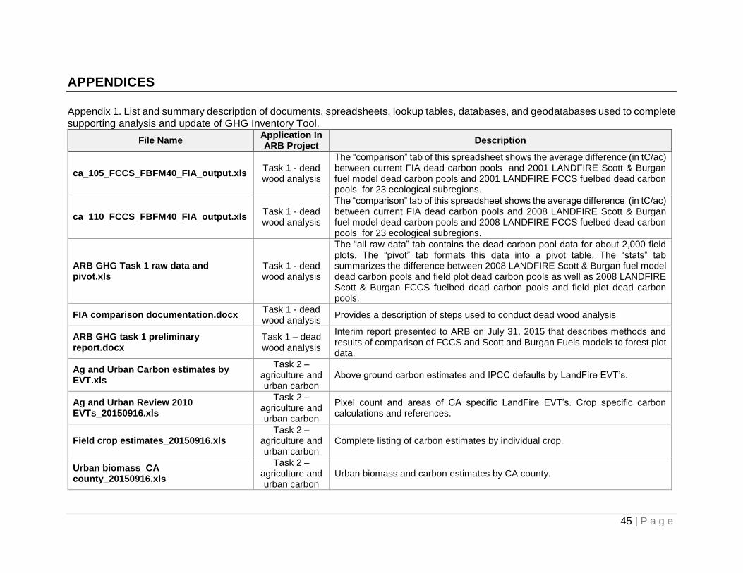
45 | P a g e
APPENDICES
Appendix 1. List and summary description of documents, spreadsheets, lookup tables, databases, and geodatabases used to complete supporting analysis and update of GHG Inventory Tool.
File Name Application In ARB Project
Description
ca_105_FCCS_FBFM40_FIA_output.xls Task 1 - dead wood analysis
The “comparison” tab of this spreadsheet shows the average difference (in tC/ac) between current FIA dead carbon pools and 2001 LANDFIRE Scott & Burgan fuel model dead carbon pools and 2001 LANDFIRE FCCS fuelbed dead carbon pools for 23 ecological subregions.
ca_110_FCCS_FBFM40_FIA_output.xls Task 1 - dead wood analysis
The “comparison” tab of this spreadsheet shows the average difference (in tC/ac) between current FIA dead carbon pools and 2008 LANDFIRE Scott & Burgan fuel model dead carbon pools and 2008 LANDFIRE FCCS fuelbed dead carbon pools for 23 ecological subregions.
ARB GHG Task 1 raw data and pivot.xls
Task 1 - dead wood analysis
The “all raw data” tab contains the dead carbon pool data for about 2,000 field plots. The “pivot” tab formats this data into a pivot table. The “stats” tab summarizes the difference between 2008 LANDFIRE Scott & Burgan fuel model dead carbon pools and field plot dead carbon pools as well as 2008 LANDFIRE Scott & Burgan FCCS fuelbed dead carbon pools and field plot dead carbon pools.
FIA comparison documentation.docx Task 1 - dead wood analysis
Provides a description of steps used to conduct dead wood analysis
ARB GHG task 1 preliminary report.docx
Task 1 – dead wood analysis
Interim report presented to ARB on July 31, 2015 that describes methods and results of comparison of FCCS and Scott and Burgan Fuels models to forest plot data.
Ag and Urban Carbon estimates by EVT.xls
Task 2 – agriculture and urban carbon
Above ground carbon estimates and IPCC defaults by LandFire EVT’s.
Ag and Urban Review 2010 EVTs_20150916.xls
Task 2 – agriculture and urban carbon
Pixel count and areas of CA specific LandFire EVT’s. Crop specific carbon calculations and references.
Field crop estimates_20150916.xls Task 2 –
agriculture and urban carbon
Complete listing of carbon estimates by individual crop.
Urban biomass_CA county_20150916.xls
Task 2 – agriculture and urban carbon
Urban biomass and carbon estimates by CA county.
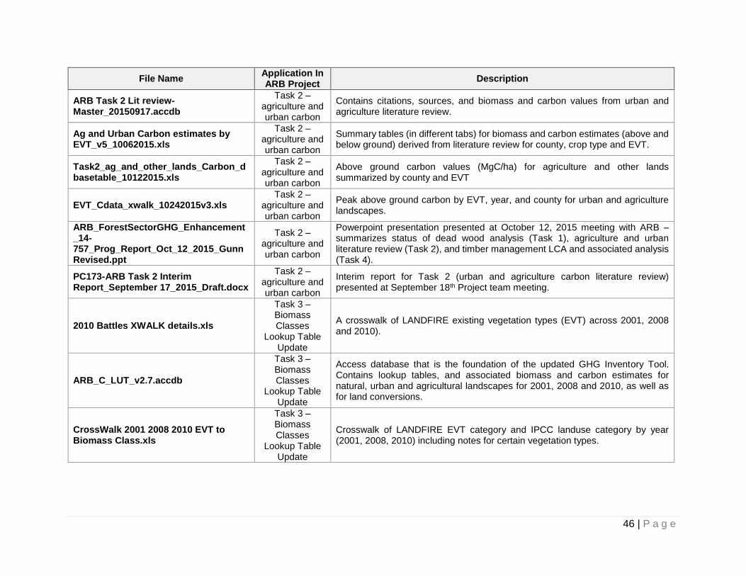
46 | P a g e
File Name Application In ARB Project
Description
ARB Task 2 Lit review-Master_20150917.accdb
Task 2 – agriculture and urban carbon
Contains citations, sources, and biomass and carbon values from urban and agriculture literature review.
Ag and Urban Carbon estimates by EVT_v5_10062015.xls
Task 2 – agriculture and urban carbon
Summary tables (in different tabs) for biomass and carbon estimates (above and below ground) derived from literature review for county, crop type and EVT.
Task2_ag_and_other_lands_Carbon_dbasetable_10122015.xls
Task 2 – agriculture and urban carbon
Above ground carbon values (MgC/ha) for agriculture and other lands summarized by county and EVT
EVT_Cdata_xwalk_10242015v3.xls Task 2 –
agriculture and urban carbon
Peak above ground carbon by EVT, year, and county for urban and agriculture landscapes.
ARB_ForestSectorGHG_Enhancement_14-757_Prog_Report_Oct_12_2015_GunnRevised.ppt
Task 2 – agriculture and urban carbon
Powerpoint presentation presented at October 12, 2015 meeting with ARB – summarizes status of dead wood analysis (Task 1), agriculture and urban literature review (Task 2), and timber management LCA and associated analysis (Task 4).
PC173-ARB Task 2 Interim Report_September 17_2015_Draft.docx
Task 2 – agriculture and urban carbon
Interim report for Task 2 (urban and agriculture carbon literature review) presented at September 18th Project team meeting.
2010 Battles XWALK details.xls
Task 3 – Biomass Classes
Lookup Table Update
A crosswalk of LANDFIRE existing vegetation types (EVT) across 2001, 2008 and 2010).
ARB_C_LUT_v2.7.accdb
Task 3 – Biomass Classes
Lookup Table Update
Access database that is the foundation of the updated GHG Inventory Tool. Contains lookup tables, and associated biomass and carbon estimates for natural, urban and agricultural landscapes for 2001, 2008 and 2010, as well as for land conversions.
CrossWalk 2001 2008 2010 EVT to Biomass Class.xls
Task 3 – Biomass Classes
Lookup Table Update
Crosswalk of LANDFIRE EVT category and IPCC landuse category by year (2001, 2008, 2010) including notes for certain vegetation types.
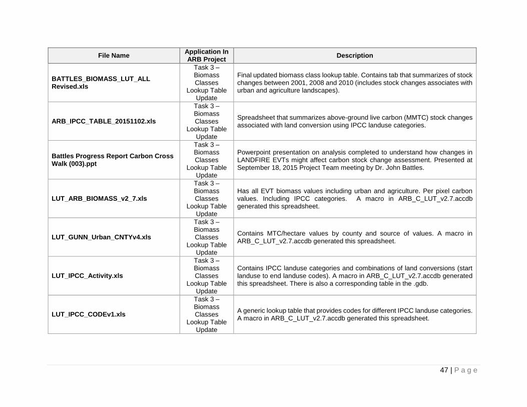
47 | P a g e
File Name Application In ARB Project
Description
BATTLES_BIOMASS_LUT_ALL Revised.xls
Task 3 – Biomass Classes
Lookup Table Update
Final updated biomass class lookup table. Contains tab that summarizes of stock changes between 2001, 2008 and 2010 (includes stock changes associates with urban and agriculture landscapes).
ARB_IPCC_TABLE_20151102.xls
Task 3 – Biomass Classes
Lookup Table Update
Spreadsheet that summarizes above-ground live carbon (MMTC) stock changes associated with land conversion using IPCC landuse categories.
Battles Progress Report Carbon Cross Walk (003).ppt
Task 3 – Biomass Classes
Lookup Table Update
Powerpoint presentation on analysis completed to understand how changes in LANDFIRE EVTs might affect carbon stock change assessment. Presented at September 18, 2015 Project Team meeting by Dr. John Battles.
LUT_ARB_BIOMASS_v2_7.xls
Task 3 – Biomass Classes
Lookup Table Update
Has all EVT biomass values including urban and agriculture. Per pixel carbon values. Including IPCC categories. A macro in ARB_C_LUT_v2.7.accdb generated this spreadsheet.
LUT_GUNN_Urban_CNTYv4.xls
Task 3 – Biomass Classes
Lookup Table Update
Contains MTC/hectare values by county and source of values. A macro in ARB_C_LUT_v2.7.accdb generated this spreadsheet.
LUT_IPCC_Activity.xls
Task 3 – Biomass Classes
Lookup Table Update
Contains IPCC landuse categories and combinations of land conversions (start landuse to end landuse codes). A macro in ARB_C_LUT_v2.7.accdb generated this spreadsheet. There is also a corresponding table in the .gdb.
LUT_IPCC_CODEv1.xls
Task 3 – Biomass Classes
Lookup Table Update
A generic lookup table that provides codes for different IPCC landuse categories. A macro in ARB_C_LUT_v2.7.accdb generated this spreadsheet.
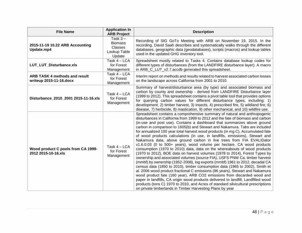
48 | P a g e
File Name Application In ARB Project
Description
2015-11-19 10.22 ARB Accounting Update.mp4
Task 3 – Biomass Classes
Lookup Table Update
Recording of SIG GoTo Meeting with ARB on November 19, 2015. In the recording, David Saah describes and systematically walks through the different databases, geographic data (geodatabases), scripts (macros) and lookup tables used in the updated GHG inventory tool.
LUT_LUT_Disturbance.xls Task 4 – LCA
for Forest Management
Spreadsheet mostly related to Tasks 4. Contains database lookup codes for different types of disturbances (from the LANDFIRE disturbance layer). A macro in ARB_C_LUT_v2.7.accdb generated this spreadsheet.
ARB TASK 4 methods and result writeup 2015-11-16.docx
Task 4 – LCA for Forest
Management
Interim report on methods and results related to harvest associated carbon losses on the landscape across California from 2001 to 2010.
Disturbance_2010_2001 2015-11-16.xls Task 4 – LCA
for Forest Management
Summary of harvest/disturbance area (by type) and associated biomass and carbon by county and ownership - derived from LANDFIRE Disturbance layer (1999 to 2012). This spreadsheet contains a pivot table tool that provides options for querying carbon values for different disturbance types, including: 1) development, 2) timber harvest, 3) insects, 4) prescribed fire, 5) wildland fire, 6) disease, 7) herbicide, 8) mastication, 9) other mechanical, and 10) wildfire use.
Wood product C pools from CA 1999-2012 2015-10-16.xls
Task 4 – LCA for Forest
Management
Spreadsheet contains a comprehensive summary of natural and anthropogenic disturbances in California from 1999 to 2012 and the fate of biomass and carbon (in-use and post use). Contains a dashboard that summarizes above ground carbon in comparison to 1605(b) and Stewart and Nakamura. Tabs are included for annualized 100 year total harvest wood products (in mg C), Accumulated fate of wood products calculations (in use, in landfills, emissions), Stewart and Nakamura data, above ground carbon in live trees from FIA EVALIDator v1.6.0.03 (0 to 500+ years), wood volume per hectare, CA wood products consumption (1970 to 2010) data, data on the whereabouts of wood products (1970 to 2012), BOE data on harvest volumes (1978 to 2014), Forest Types by ownership and associated volumes (source FIA), USFS PNW Ca. timber harvest (mmbf) by ownership (1952-2008), log exports (mmbf) 1961 to 2012, decadal CA census data (1850 to 2010), timber consumption data (1965 to 2002), Smith et al. 2006 wood product fractional C emissions (96 years), Stewart and Nakamura wood product fate (160 year), ARB CO2 emissions from discarded wood and paper in landfills, CA origin wood products delivered to landfill, Landfilled wood products (tons C) 1970 to 2010, and Acres of standard silvicultural prescriptions on private timberlands in Timber Harvesting Plans by year
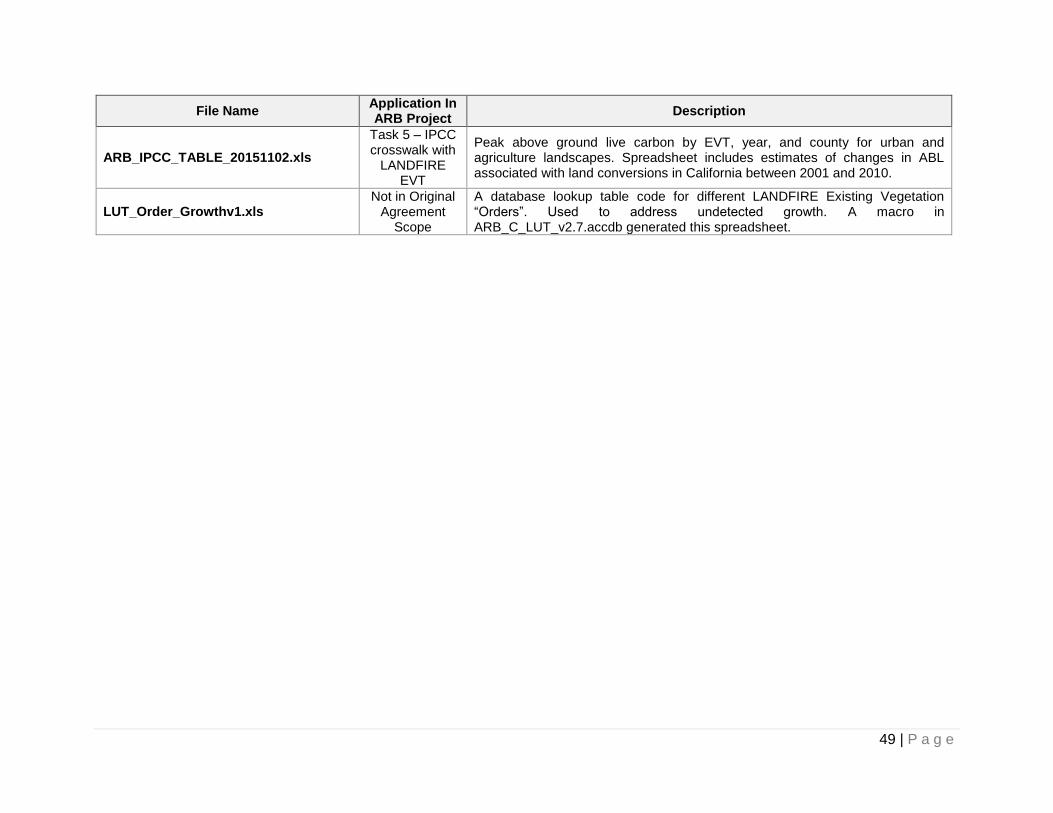
49 | P a g e
File Name Application In ARB Project
Description
ARB_IPCC_TABLE_20151102.xls
Task 5 – IPCC crosswalk with
LANDFIRE EVT
Peak above ground live carbon by EVT, year, and county for urban and agriculture landscapes. Spreadsheet includes estimates of changes in ABL associated with land conversions in California between 2001 and 2010.
LUT_Order_Growthv1.xls Not in Original
Agreement Scope
A database lookup table code for different LANDFIRE Existing Vegetation “Orders”. Used to address undetected growth. A macro in ARB_C_LUT_v2.7.accdb generated this spreadsheet.
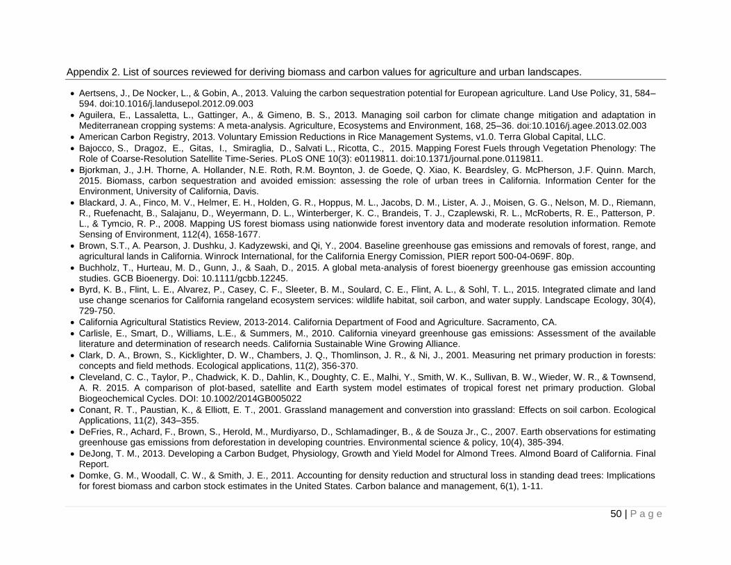
50 | P a g e
Appendix 2. List of sources reviewed for deriving biomass and carbon values for agriculture and urban landscapes.
Aertsens, J., De Nocker, L., & Gobin, A., 2013. Valuing the carbon sequestration potential for European agriculture. Land Use Policy, 31, 584–594. doi:10.1016/j.landusepol.2012.09.003
Aguilera, E., Lassaletta, L., Gattinger, A., & Gimeno, B. S., 2013. Managing soil carbon for climate change mitigation and adaptation in Mediterranean cropping systems: A meta-analysis. Agriculture, Ecosystems and Environment, 168, 25–36. doi:10.1016/j.agee.2013.02.003
American Carbon Registry, 2013. Voluntary Emission Reductions in Rice Management Systems, v1.0. Terra Global Capital, LLC.
Bajocco, S., Dragoz, E., Gitas, I., Smiraglia, D., Salvati L., Ricotta, C., 2015. Mapping Forest Fuels through Vegetation Phenology: The Role of Coarse-Resolution Satellite Time-Series. PLoS ONE 10(3): e0119811. doi:10.1371/journal.pone.0119811.
Bjorkman, J., J.H. Thorne, A. Hollander, N.E. Roth, R.M. Boynton, J. de Goede, Q. Xiao, K. Beardsley, G. McPherson, J.F. Quinn. March, 2015. Biomass, carbon sequestration and avoided emission: assessing the role of urban trees in California. Information Center for the Environment, University of California, Davis.
Blackard, J. A., Finco, M. V., Helmer, E. H., Holden, G. R., Hoppus, M. L., Jacobs, D. M., Lister, A. J., Moisen, G. G., Nelson, M. D., Riemann, R., Ruefenacht, B., Salajanu, D., Weyermann, D. L., Winterberger, K. C., Brandeis, T. J., Czaplewski, R. L., McRoberts, R. E., Patterson, P. L., & Tymcio, R. P., 2008. Mapping US forest biomass using nationwide forest inventory data and moderate resolution information. Remote Sensing of Environment, 112(4), 1658-1677.
Brown, S.T., A. Pearson, J. Dushku, J. Kadyzewski, and Qi, Y., 2004. Baseline greenhouse gas emissions and removals of forest, range, and agricultural lands in California. Winrock International, for the California Energy Comission, PIER report 500-04-069F. 80p.
Buchholz, T., Hurteau, M. D., Gunn, J., & Saah, D., 2015. A global meta‐analysis of forest bioenergy greenhouse gas emission accounting studies. GCB Bioenergy. Doi: 10.1111/gcbb.12245.
Byrd, K. B., Flint, L. E., Alvarez, P., Casey, C. F., Sleeter, B. M., Soulard, C. E., Flint, A. L., & Sohl, T. L., 2015. Integrated climate and land use change scenarios for California rangeland ecosystem services: wildlife habitat, soil carbon, and water supply. Landscape Ecology, 30(4), 729-750.
California Agricultural Statistics Review, 2013-2014. California Department of Food and Agriculture. Sacramento, CA.
Carlisle, E., Smart, D., Williams, L.E., & Summers, M., 2010. California vineyard greenhouse gas emissions: Assessment of the available literature and determination of research needs. California Sustainable Wine Growing Alliance.
Clark, D. A., Brown, S., Kicklighter, D. W., Chambers, J. Q., Thomlinson, J. R., & Ni, J., 2001. Measuring net primary production in forests: concepts and field methods. Ecological applications, 11(2), 356-370.
Cleveland, C. C., Taylor, P., Chadwick, K. D., Dahlin, K., Doughty, C. E., Malhi, Y., Smith, W. K., Sullivan, B. W., Wieder, W. R., & Townsend, A. R. 2015. A comparison of plot‐based, satellite and Earth system model estimates of tropical forest net primary production. Global Biogeochemical Cycles. DOI: 10.1002/2014GB005022
Conant, R. T., Paustian, K., & Elliott, E. T., 2001. Grassland management and converstion into grassland: Effects on soil carbon. Ecological Applications, 11(2), 343–355.
DeFries, R., Achard, F., Brown, S., Herold, M., Murdiyarso, D., Schlamadinger, B., & de Souza Jr., C., 2007. Earth observations for estimating greenhouse gas emissions from deforestation in developing countries. Environmental science & policy, 10(4), 385-394.
DeJong, T. M., 2013. Developing a Carbon Budget, Physiology, Growth and Yield Model for Almond Trees. Almond Board of California. Final Report.
Domke, G. M., Woodall, C. W., & Smith, J. E., 2011. Accounting for density reduction and structural loss in standing dead trees: Implications for forest biomass and carbon stock estimates in the United States. Carbon balance and management, 6(1), 1-11.
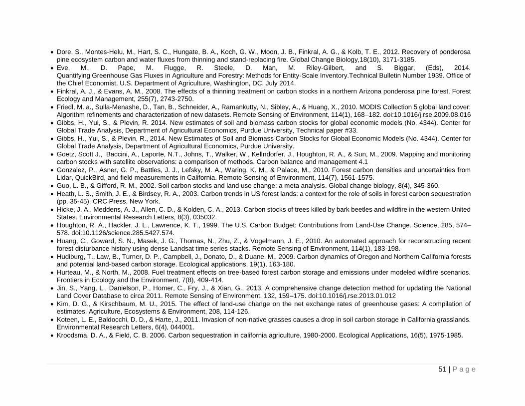
51 | P a g e
Dore, S., Montes‐Helu, M., Hart, S. C., Hungate, B. A., Koch, G. W., Moon, J. B., Finkral, A. G., & Kolb, T. E., 2012. Recovery of ponderosa pine ecosystem carbon and water fluxes from thinning and stand‐replacing fire. Global Change Biology,18(10), 3171-3185.
Eve, M., D. Pape, M. Flugge, R. Steele, D. Man, M. Riley‐Gilbert, and S. Biggar, (Eds), 2014. Quantifying Greenhouse Gas Fluxes in Agriculture and Forestry: Methods for Entity‐Scale Inventory.Technical Bulletin Number 1939. Office of the Chief Economist, U.S. Department of Agriculture, Washington, DC. July 2014.
Finkral, A. J., & Evans, A. M., 2008. The effects of a thinning treatment on carbon stocks in a northern Arizona ponderosa pine forest. Forest Ecology and Management, 255(7), 2743-2750.
Friedl, M. a., Sulla-Menashe, D., Tan, B., Schneider, A., Ramankutty, N., Sibley, A., & Huang, X., 2010. MODIS Collection 5 global land cover: Algorithm refinements and characterization of new datasets. Remote Sensing of Environment, 114(1), 168–182. doi:10.1016/j.rse.2009.08.016
Gibbs, H., Yui, S., & Plevin, R. 2014. New estimates of soil and biomass carbon stocks for global economic models (No. 4344). Center for Global Trade Analysis, Department of Agricultural Economics, Purdue University, Technical paper #33.
Gibbs, H., Yui, S., & Plevin, R., 2014. New Estimates of Soil and Biomass Carbon Stocks for Global Economic Models (No. 4344). Center for Global Trade Analysis, Department of Agricultural Economics, Purdue University.
Goetz, Scott J., Baccini, A., Laporte, N.T., Johns, T., Walker, W., Kellndorfer, J., Houghton, R. A., & Sun, M., 2009. Mapping and monitoring carbon stocks with satellite observations: a comparison of methods. Carbon balance and management 4.1
Gonzalez, P., Asner, G. P., Battles, J. J., Lefsky, M. A., Waring, K. M., & Palace, M., 2010. Forest carbon densities and uncertainties from Lidar, QuickBird, and field measurements in California. Remote Sensing of Environment, 114(7), 1561-1575.
Guo, L. B., & Gifford, R. M., 2002. Soil carbon stocks and land use change: a meta analysis. Global change biology, 8(4), 345-360.
Heath, L. S., Smith, J. E., & Birdsey, R. A., 2003. Carbon trends in US forest lands: a context for the role of soils in forest carbon sequestration (pp. 35-45). CRC Press, New York.
Hicke, J. A., Meddens, A. J., Allen, C. D., & Kolden, C. A., 2013. Carbon stocks of trees killed by bark beetles and wildfire in the western United States. Environmental Research Letters, 8(3), 035032.
Houghton, R. A., Hackler, J. L., Lawrence, K. T., 1999. The U.S. Carbon Budget: Contributions from Land-Use Change. Science, 285, 574–578. doi:10.1126/science.285.5427.574.
Huang, C., Goward, S. N., Masek, J. G., Thomas, N., Zhu, Z., & Vogelmann, J. E., 2010. An automated approach for reconstructing recent forest disturbance history using dense Landsat time series stacks. Remote Sensing of Environment, 114(1), 183-198.
Hudiburg, T., Law, B., Turner, D. P., Campbell, J., Donato, D., & Duane, M., 2009. Carbon dynamics of Oregon and Northern California forests and potential land-based carbon storage. Ecological applications, 19(1), 163-180.
Hurteau, M., & North, M., 2008. Fuel treatment effects on tree-based forest carbon storage and emissions under modeled wildfire scenarios. Frontiers in Ecology and the Environment, 7(8), 409-414.
Jin, S., Yang, L., Danielson, P., Homer, C., Fry, J., & Xian, G., 2013. A comprehensive change detection method for updating the National Land Cover Database to circa 2011. Remote Sensing of Environment, 132, 159–175. doi:10.1016/j.rse.2013.01.012
Kim, D. G., & Kirschbaum, M. U., 2015. The effect of land-use change on the net exchange rates of greenhouse gases: A compilation of estimates. Agriculture, Ecosystems & Environment, 208, 114-126.
Koteen, L. E., Baldocchi, D. D., & Harte, J., 2011. Invasion of non-native grasses causes a drop in soil carbon storage in California grasslands. Environmental Research Letters, 6(4), 044001.
Kroodsma, D. A., & Field, C. B. 2006. Carbon sequestration in california agriculture, 1980-2000. Ecological Applications, 16(5), 1975-1985.
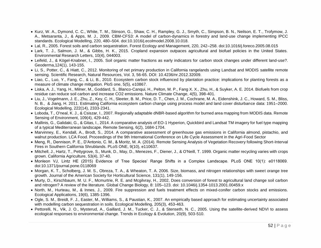
52 | P a g e
Kurz, W. A., Dymond, C. C., White, T. M., Stinson, G., Shaw, C. H., Rampley, G. J., Smyth, C., Simpson, B. N., Neilson, E. T., Trofymow, J. A., Metsaranta, J., & Apps, M. J., 2009. CBM-CFS3: A model of carbon-dynamics in forestry and land-use change implementing IPCC standards. Ecological Modelling, 220, 480–504. doi:10.1016/j.ecolmodel.2008.10.018.
Lal, R., 2005. Forest soils and carbon sequestration. Forest Ecology and Management, 220, 242–258. doi:10.1016/j.foreco.2005.08.015
Lark, T. J., Salmon, J. M., & Gibbs, H. K., 2015. Cropland expansion outpaces agricultural and biofuel policies in the United States. Environmental Research Letters, 10(4), 044003.
Leifeld, J., & Kögel-Knabner, I., 2005. Soil organic matter fractions as early indicators for carbon stock changes under different land-use?. Geoderma,124(1), 143-155.
Li, S., Potter, C., & Hiatt, C., 2012. Monitoring of net primary production in California rangelands using Landsat and MODIS satellite remote sensing. Scientific Research, Natural Resources, Vol. 3, 56-65. DOI: 10.4236/nr.2012.32009.
Liao, C., Luo, Y., Fang, C., & Li, B., 2010. Ecosystem carbon stock influenced by plantation practice: implications for planting forests as a measure of climate change mitigation. PloS one, 5(5), e10867.
Liska, A. J., Yang, H., Milner, M., Goddard, S., Blanco-Canqui, H., Pelton, M. P., Fang X. X., Zhu, H., & Suyker, A. E. 2014. Biofuels from crop residue can reduce soil carbon and increase CO2 emissions. Nature Climate Change, 4(5), 398-401.
Liu, J., Vogelmann, J. E., Zhu, Z., Key, C. H., Sleeter, B. M., Price, D. T., Chen, J. M., Cochrane, M. A., Eidenshink, J. C., Howard, S. M., Bliss, N. B., & Jiang, H. 2011. Estimating California ecosystem carbon change using process model and land cover disturbance data: 1951–2000. Ecological Modelling, 222(14), 2333-2341.
Loboda, T., O'neal, K. J., & Csiszar, I., 2007. Regionally adaptable dNBR-based algorithm for burned area mapping from MODIS data. Remote Sensing of Environment, 109(4), 429-442.
Mallinis, G., Galidaki, G., & Gitas, I., 2014. A comparative analysis of EO-1 Hyperion, Quickbird and Landsat TM imagery for fuel type mapping of a typical Mediterranean landscape. Remote Sensing, 6(2), 1684-1704.
Marvinney, E., Kendall, A., Brodt, S., 2014. A comparative assessment of greenhouse gas emissions in California almond, pistachio, and walnut production. LCA Food. Proceedings of the 9th International Conference on Life Cycle Assessment in the Agri-Food Sector
Meng, R., Dennison, P. E., D’Antonio, C. M., & Moritz, M. A. (2014). Remote Sensing Analysis of Vegetation Recovery following Short-Interval Fires in Southern California Shrublands. PLoS ONE, 9(10), e110637.
Mitchell, J., Hartz, T., Pettygrove, S., Munk, D., May, D., Menezes, F., Diener, J., & O'Neill, T. 1999. Organic matter recycling varies with crops grown. California Agriculture, 53(4), 37-40.
Monleon VJ, Lintz HE (2015) Evidence of Tree Species’ Range Shifts in a Complex Landscape. PLoS ONE 10(1): e0118069. doi:10.1371/journal.pone.0118069
Morgan, K. T., Scholberg, J. M. S., Obreza, T. A., & Wheaton, T. A. 2006. Size, biomass, and nitrogen relationships with sweet orange tree growth. Journal of the American Society for Horticultural Science, 131(1), 149-156.
Murty, D., Kirschbaum, M. U. F., Mcmurtrie, R. E. and Mcgilvray, H., 2002, Does conversion of forest to agricultural land change soil carbon and nitrogen? A review of the literature. Global Change Biology, 8: 105–123. doi: 10.1046/j.1354-1013.2001.00459.x
North, M., Hurteau, M., & Innes, J., 2009. Fire suppression and fuels treatment effects on mixed-conifer carbon stocks and emissions. Ecological Applications, 19(6), 1385-1396.
Ogle, S. M., Breidt, F. J., Easter, M., Williams, S., & Paustian, K., 2007. An empirically based approach for estimating uncertainty associated with modelling carbon sequestration in soils. Ecological Modelling, 205(3), 453-463.
Pettorelli, N., Vik, J. O., Mysterud, A., Gaillard, J. M., Tucker, C. J., & Stenseth, N. C., 2005. Using the satellite-derived NDVI to assess ecological responses to environmental change. Trends in Ecology & Evolution, 20(9), 503-510.
53 | P a g e
Plevin, R. J., O'Hare, M., Jones, A. D., Torn, M. S., & Gibbs, H. K., 2010. Greenhouse gas emissions from biofuels’ indirect land use change are uncertain but may be much greater than previously estimated. Environmental Science and Technology, 44(21), 8015–8021. doi:10.1021/es101946t
Potter, C., 2012. Net primary production and carbon cycling in coast redwood forests of central California. Open Journal of Ecology.
Putnam, Daniel H. 2015. Alfalfa and Foreage News. UC Cooperative Extension: http://ucanr.edu/blogs/blogcore/postdetail.cfm?postnum=17721
Rosecrance, R. and Lovatt, C. 2003. Seasonal Patterns of Nutrient Uptake and Partitioning as a Function of Crop Load of the 'Hass' avocado. CSU, Chico. Final Report.
Roy, D.P., Ju, J., Kline, K., Scaramuzza, P.L., Kovalskyy, V., Hansen, M.C., Loveland, T.R., Vermote, E.F., Zhang, C., 2010, Web-enabled Landsat Data (WELD): Landsat ETM+ Composited Mosaics of the Conterminous United States. Remote Sensing of Environment 114: 35-49.
Ryals, R., & Silver, W. L. 2013. Effects of organic matter amendments on net primary productivity and greenhouse gas emissions in annual grasslands. Ecological Applications, 23(1), 46-59.
Ryan, K. C., & Opperman, T. S., 2013. LANDFIRE - A national vegetation/fuels data base for use in fuels treatment, restoration, and suppression planning. Forest Ecology and Management, 294, 208–216. doi:10.1016/j.foreco.2012.11.003
Seto, K. C., Fragkias, M., Güneralp, B., & Reilly, M. K., 2011. A meta-analysis of global urban land expansion. PloS ONE, 6(8), e23777. doi:10.1371/journal.pone.0023777.
Silver, W. L., Ryals, R., & Eviner, V., 2010. Soil carbon pools in California's annual grassland ecosystems. Rangeland Ecology & Management, 63(1), 128-136.
Smith, J. E., Heath, L. S., & Woodbury, P. B., 2004. How to estimate forest carbon for large areas from inventory data. Journal of Forestry, 102(5), 25-31.
Smith, James E., Heath, Linda S., Skog, Kenneth E., Birdsey, Richard A. 2006. Methods for calculating forest ecosystem and harvested carbon with standard estimates for forest types of the United States. Gen. Tech. Rep. NE-343. Newtown Square, PA: U.S. Department of Agriculture, Forest Service, Northeastern Research Station. 216 p.
Springsteen, B., Christofk, T., Eubanks, S., Mason, T., Clavin, C., & Storey, B., 2011. Emission reductions from woody biomass waste for energy as an alternative to open burning. Journal of the Air & Waste Management Association, 61(1), 63-68. DOI: 10.3155/1047-3289.61.1.63.
Stevens, A., van Wesemael, B., Vandenschrick, G., Touré, S., & Tychon, B., 2006. Detection of Carbon Stock Change in Agricultural Soils Using Spectroscopic Techniques. Soil Science Society of America Journal, 70, 844. doi:10.2136/sssaj2005.0025
T. M. Dejong, 2013. Developing a Carbon Budget, Physiology, Growth, and Yield Potential Model for Almond Trees. Project Final Report, Plant Sciences Department, UC Davis.
Turner, D.P., W.D. Ritts, W.B. Cohen, S.T. Gower, S.W. Running, M. Zhao, M.H. Costa, A. Kirschbaum, J. Ham, S. Saleska, and D.E. Ahl. 2006. Evaluation of MODIS NPP and GPP products across multiple biomes. Remote Sensing of Environment 102: 282-292.
van Kooten, G. C., Eagle, A. J., Manley, J., & Smolak, T., 2004. How costly are carbon offsets? A meta-analysis of carbon forest sinks. Environmental Science & Policy, 7(4), 239-251.
Vashum, K. T., & Jayakumar, S., 2012. Methods to estimate above-ground biomass and carbon stock in natural forests-a review. Journal of Ecosystem & Ecography, 2(116), 1-7.
Warner, E., Inman, D., Kunstman, B., Bush, B., Vimmerstedt, L., Peterson, S., Macknick, J., & Zhang, Y., 2013. Modeling biofuel expansion effects on land use change dynamics. Environmental Research Letters, 8(1), 015003.
54 | P a g e
West, T. O., Brandt, C. C., Baskaran, L. M., Hellwinckel, C. M., Mueller, R., Bernacchi, C. J., Bandaru, V., Yang, B., Wilson, B. S., Marland, G., Nelson, R. G., De La Torre Ugarte, D. G., & Post, W. M. 2010. Cropland carbon fluxes in the United States: increasing geospatial resolution of inventory-based carbon accounting. Ecological Applications, 20(4), 1074-1086.
Wilson, B. T., Woodall, C. W., & Griffith, D. M., 2013. Imputing forest carbon stock estimates from inventory plots to a nationally continuous coverage. Carbon Balance Management, 8(1).
Woodall, C. W., Domke, G. M., Macfarlane, D. W., & Oswalt, C. M., 2012. Comparing field-and model-based standing dead tree carbon stock estimates across forests of the US. Forestry, 85(1), 125-133.
Woodbury, P. B., Smith, J. E., & Heath, L. S., 2007. Carbon sequestration in the US forest sector from 1990 to 2010. Forest Ecology and Management, 241(1), 14-27.
Woodwell, G. M., Hobbie, J. E., Houghton, R. A., Melillo, J. M., Moore, B., Peterson, B. J., & Shaver, G. R., 1983. Global deforestation: contribution to atmospheric carbon dioxide. Science, 222(4628), 1081-1086
Wulder, M. A., White, J. C., Goward, S. N., Masek, J. G., Irons, J. R., Herold, M., Cohen, W. B., Loveland, T. R., & Woodcock, C. E., 2008. Landsat continuity: Issues and opportunities for land cover monitoring. Remote Sensing of Environment, 112(3), 955-969.
Xu, L., & Baldocchi, D. D., 2004. Seasonal variation in carbon dioxide exchange over a Mediterranean annual grassland in California. Agricultural and Forest Meteorology, 123(1), 79-96.
Yang, X., Tang, J., Mustard, J. F., Lee, J. E., Rossini, M., Joiner, J., Munger, J. W., Kornfeld, A., & Richardson, A. D., 2015. Solar‐induced chlorophyll fluorescence that correlates with canopy photosynthesis on diurnal and seasonal scales in a temperate deciduous forest. Geophysical Research Letters.