Embed Size (px)
Citation preview

AEDC-TR-91-26 "~-~2,'1 '[~-~"[ I I I VOLUME I " ~ ~"
New Technology for Remote Testing of Response Time
]1[ of Installed Thermocouples
i ~ Volume I - - Background and General Details , 3 ,
H. M. Hashemian Analysis and Measurement Services Corp.
AMS 9111 Cross Park Dr., N. W. Knoxville, TN 37923
January 1992
Final Report for Period September 1987 - December 1990
PROPERTY OF U.S. AIR FORCE AF.DC TF.CHNICki. liBRARY
Approvecl for public release: dlStrlbutmn IS unhmlted, i
TECHNICAL ~EPORTS ¥ ! L ~ COPY
ARNOLD ENGINEERING DEVELOPMENT CENTER ARNOLD AIR FORCE BASE, TENNESSEE
AIR FORCE SYSTEMS COMMAND UNITED STATES AIR FORCE

NOTICES
When U. S. Govmnne~t drawinlls, specifications, or other data me used for any purpose other than a definitely related Government procuremmt OlX~tioa, the Government thereby incurs no responsFoility nor any obligation whatsoever, and the fact that the Governmeat may have formulated, furnished, or in any way supplied the said drawings, specifications, or other data, is not to be resarded by implication or otherwise, or in any manner licensing the holder or any other person or corporation, or conveyin8 any rishts or permission to manufacture, use, or sell any patented invention that may in any way be related thereto.
Qualified users m y obtain copies of this report from the Defense Technical Information Center.
References to named commercial products in this report are not to be considered in any sense as an endorsement of the product by the United States Air Force or the Government.
This report has been reviewed by the Office of Public Affairs (PA) and is releasable to the National Technical Information Service (NTIS). At NTIS, it will be available to the general public, including foreign nations.
Reproducibles used in the publication of this report were supplied by the authors. AEDC has neither edited nor altered this manuscript.
APPROVAL STATEMENT
This report has been reviewed and approved.
SETH SHEPHERD, Capt, USAF Facility Technology Division Directorate of Technology Deputy for Operations
Approved for publication:
FOR THE COMMANDER
KEITH L. KUSHMAN Director of Technology Deputy for Operations

Form Approved REPORT DOCUMENTATION PAGE OMB No. 0704-0188
i
Public reporting burden for tl~s ¢ollecl~on of iofmmsbon Is eillmated to average 1 hour per response. Including the time for reviewing Imtructlons. searching ernstlng data sources, gathedng and maintaining the data needed, and completing and revlewng the collection of I n f o r m , Send comments regarding this burden esllmale or any other aspect of this collection of Infermatloa, Including suggestiorn for rnduong this buude~, toWmihlngton Heedquerlm 5ervKes. Directorate for Inforrnabon OlperatN)ns and Reports, 1215 Jefferlon Oasis Hucjhway r Suite T204 r Arlington r VA )):n:-4S02 r and to the OItlce of Manml. ement and a~l~m~! paperwork Reduction proJecl ~o4.0 lea). Washlncllon. DC 2050S.
1.AGENCY USE ONLY(Leave bJank) I 2. REPORT DATE | 3. REPORTTYPE AND DATESCOVERED . • I January 1992 I Final, september 1987 - December 1990
4. TITLE AND SUBTITLE S. FUNDING NUMBERS New Technology for Remote Testing of Response Time of Installed Thermocouples, Vol. I, Background and General Details F40600-87-C0003
6. AUTHOR(S)
Hashemian, H. M. Analysis and Measurement Services Corp. 7. PERFORMING ORGANIZATION NAME(S)AND ADDRESS(ES)
Analysis and Measurement Services Corp. AMS 9111 Cross Park Drive, N.W. Knoxville, TN 37923-4599
9. SPONSORING/MONITORING AGENCY NAMES(S) AND ADDRESS(ES)
Arnold Engineering Development Center/DOT Air Force Systems Command Arnold Air Force Base, TN 37389-5000
8. PERFORMING ORGANIZATION REPORT NUMBER
AEDC-TR-91-26, Vol. I
10. SPONSORING/MONITORING AGENCY REPORT NUMBER
11. SUPPLEMENTARY NOTES Available in Defense Technical Information Center (DTIC).
12a. DISTRIBUTION/AVAILABILITY STATEMENT
Approved for public release; distribution is unlimited.
12b. DISTRIBUTION CODE
13. ABSTRACT (Maxim um 200 words) A comprehensive research and development project was completed to provide new
technology for remote testing of response time of thermocouples as installed in operating processes.
A significant portion of this development depended on the Loop Current Step Response {LCSR) method. This method is based on heating the thermocouple internally by applying an electric current to its extension leads. The current produces Joule heating in the thermocouple and causes the thermocouple junction to settle several degrees above the ambient temperature. The current is then cut off and the thermocouple output is recorded as it cools to the ambient temperature. It has been established by experimental research and theoretical development carried out in this project that this cooling transient can be i analyzed to provide the response time of the thermocouple under the conditions tested, i
With little additional effort, the equipment that was developed in this project can be adapted to provide a capability for in-situ assessment of static health, reliability, and accuracy of installed thermocouples. 14. SUBJECTTERMS thermocouple, time constant, response time, aerospace, Loop Current Step Response Method, smart sensor, in-situ testing, accuracy
17. SECURITY CLASSIFICATION OF REPORT
UNCLASSIFI ED COMPUTER GENERATED
18. SECURITY CLASSIFICATION OF THIS PAGE
UNCLASSIFIED
1S. NUMBEROF PAGES 235
16. PRICE CODE
19. SECURITY CLASSIFICATION 20. LIMITATION OF ABSTRACT OFABSTRACT SAME AS REPORT
UNCLASSIFIED Standard Form 298 (Ray, 2-89) prelolbed by ANSi S~l 7-'1-111 298-102

AEDC-TR-91-26
I
PREFACE
This is Volume I of a three volume report prepared by Analysis and Measurement
Services Corporation (AMS) for Arnold Engineering Development Center, Air Force Systems
Command, Arnold Air Force Station, Tennessee. The report has been written as an account of
work completed over a three year period under contract number F40600-87-C0003. The Air
Force project manager was Mr. Robert W. Smith, AEDC/DOT. The report has been written by
H. M. Hashemlan of Analysis and Measurement Services Corporation.
This volume contains the background of the project, the theoretical aspects of the
research and development carried out, and a summary of the key research results along with a
description of the test equipment developed. Volume I] contains the supporting research data,
details on how the research was carded out, and a description of the equipment and procedures
that were used in performing the work.
Volume II1 contains a detailed description of the test equipment that was developed in
this project. It inCludes an operations and maintenance manual for the equipment, software flow
charts and listings, parts list, drawings, photographs, and other details.

AEDC-TR-91-26
ABSTRACT
A comprehensive research and development project was successfully carried out to
provide new technology for in-situ response time testing of thermocouples as installed in
operating processes. The details are presented in this report.
This development was based on the Loop Current Step Response (LCSR) method. This
method permits remote testing of installed thermocouplas under process operating conditions.
This capability is useful in all applications involving transient temperature measurements with
thermocouples. Presently, transient temperature measurements are often restricted to small
thermocouples that can be assumed to have a negligible response time. One advantage of the
LCSR test is that it eliminates such restrictions by providing a means to measure and correct for
the delay of the thermocouple. Another advantage is that it provides a tool for checking the
installation integrity and to account for aging effects on response time of thermocouplas that are
used in hostile environments.
The response time of a thermocouple Js normally measured from its transient output when
the temperature of the environment is changed. In the LCSR test, the same response time is
determined by analysis of a transient that results from a change in temperature inside the
thermocouple. The change in temperature inside the thermocouple is induced by applying an
electric current to the thermocouple's extension leads.
The validity and the accuracy of the LCSR test for measurement of response time of
thermocouples was established in this project. The results of the validation work were used as
a guide in the design of optimum test equipment that was constructed in this project to
implement the LCSR test in aerospace and other applications.

AEDC-TR-91-26
,
2.
3.
4
5.
,
.
,
.
10.
11.
TABLE OF CONTENTS
Section Paae
11 Introduction .....................................................
Historical Perspective ......................................... • . . . . . 13
Defining Thermocouple Performance .................................. 14
Comparison of Tharmocouples With RTDs . . . . . . . . . . . . . . . . . . . . . . . . . . . . . . 18
Physical Characteristics of Thermocouples . . . . . . . . . . . . . . . . . . . . . . . . . . . . . . 23 5.1 Junction Styles ............................................. 26 5.2 Standardized Thermocouples .................................. 29 5,3 Thermocouple Extension Wires ................................. 32 5.4 Reference Junction Compensation . . . . . . . . . . . . . . . . . . . . . . . . . . . . . . 33
Thermocouple Calibration ........................................... 39 6.1 Calibration Procedure ........................................ 39 6.2 Processing of Calibration Data ................................. 45
Principles of Thermoelectric Thermometry ............................... 48 7.1 Thermoelectric Effects ........................................ 48 7.2 The Laws of Thermoelectricity .................................. -50 7.3 Thermocouple Circuit Analysis .................................. 52
Fundamentals of Sensor Dynamics .................................... 58 8.1 Response of a Simple Thermal System . . . . . . . . . . . . . . . . . . . . . . . . . . . 59 8.2 Characteristics of First Order Systems . . . . . . . . . . . . . . . . . . . . . . . . . . . . 69 8.3 Definition of Time Constant .................................... 70 8.4 Response of Higher Order Systems . . . . . . . . . . . . . . . . . . . . . . . . . . . . . . 73
Response Time Testing Methods ..................................... 79 9.1 Plunge Test ................................................ 79 9.2 Loop Current Step Response Test ............................... 86
Loop Current Step Response Theory .................................. 94 10,1 Background ................................................ 94 10.2 Heat Transfer Analysis of a Thermocouple System . . . . . . . . . . . . . . . . . . . 94 10,3 LCSR Equation ............................................. 100 10,4 Plunge Test Equation ........................................ 1 0 1
10,5 LCSR Transformation Procedure ................................ 103 10,6 Two Dimensional Heat Transfer ................................. 105
Effect of Process Conditions on Response Time . . . . . . . . . . . . . . . . . . . . . . . . . . 106 11.1 Technical Background ........................................ 106 11.2 Response Time Versus Heat Transfer Coefficient . . . . . . . . . . . . . . . . . . . . 107 11.3 Response Time Versus Flow Correlation . . . . . . . . . . . . . . . . . . . . . . . . . . 112 11.4 General Effects of Temperature on Response Time . . . . . . . . . . . . . . . . . . 114 11.5 Effect of Temperature on Heat Transfer Coefficient . . . . . . . . . . . . . . . . . . 118
AEDC-TR-91-28
12.
13.
14.
15.
16.
17.
16.
19.
20,
LCSR Validation 12.1 12.2 12.3 12.4 12.5 12.6 12.7 12.8 12.9 12.10 12.11 12.12
TABLE OF CONTENTS (continued)
.................................................. 121 Validation Results in Laboratory Conditions . . . . . . . . . . . . . . . . . . . . . . . . 123 Validation Results in Wind Tunnels . . . . . . . . . . . . . . . . . . . . . . . . . . . . . . 130 LCSR Software Qualification ................................... 133 LCSR Noise Reduction ....................................... 137 Averaging of LCSR Data ...................................... 139 LCSR Parameter Optimization .................................. 142 LCSR Difficulties ............................................ 148 LCSR Test for Detection of Thermocouple Inhomogeneitles . . . . . . . . . . . . 153 Effect of Extension Wire and Connectors . . . . . . . . . . . . . . . . . . . . . . . . . . 153 Harmful Effects of LCSR Test ................................... 156 Description of Project Thermocouples . . . . . . . . . . . . . . . . . . . . . . . . . . . . 158 Effect of Heating Time on LCSR Results . . . . . . . . . . . . . . . . . . . . . . . . . . 158
LCSR Test Instrument .............................................. 163 13.1 DescdpUon of Individual Components of LCSR Test Instrument . . . . . . . . . 172 13.2 Instrument Qualification Testing ................................. 176 13.3 Repeatability of LCSR Test Results . . . . . . . . . . . . . . . . . . . . . . . . . . . . . . 181
Factors Affecting Response Time ..................................... 184 14.1 Effect of Process Flow and Temperature . . . . . . . . . . . . . . . . . . . . . . . . . . 184 14.2 Response Time Versus Outside Diameter . . . . . . . . . . . . . . . . . . . . . . . . . 188 14.3 Effect of Temperature on Response Time . . . . . . . . . . . . . . . . . . . . . . . . . 192
Thermocouple Calibration ........................................... 197 15.1 Thermocouple Inhomogeneity Test . . . . . . . . . . . . . . . . . . . . . . . . . . . . . . 197 15.2 Short-Ranged Ordering Phenomenon . . . . . . . . . . . . . . . . . . . . . . . . . . . . 200 15.3 Effect of LCSR on Calibration of Thermocouples . . . . . . . . . . . . . . . . . . . . 203 15.4 Stability of Thermocouples ..................................... 206 15.5 Thermocouple Nonlinearities ................................... 208
Response Time Testing Using Noise Analysis . . . . . . . . . . . . . . . . . . . . . . . . . . . . 213
Test of the Installation Integrity of Thermocouples . . . . . . . . . . . . . . . . . . . . . . . . . 217
Smart Thermocouple System ........................................ 221 18,1 Testing the Condition of Installed Thermocouples . . . . . . . . . . . . . . . . . . . 221 18.2 Thermocouple Cross Calibration ................................ 223 18.3 A Smart Thermocouple System ................................. 226
Industrial Applications of LCSR Test . . . . . . . . . . . . . . . . . . . . .~ . . . . . . . . . . . . . . 228 19.1 General Applications ......................................... 228 19.2 Aerospace Applications ....................................... 228
Conclusions ..................................................... 230
REFERENCES ................................................... 231

AEDC-TR-91-26
3.1 3.2 4.1 4.2 5.1 5.2 5.3 5.4 5.5
5.6 5.7
'5.8 6.1 6.2 7.1 7.2 7.3 7.4 7.5 8.1 8.2 8.3 8.4 8.5 8.6 8.7 8.8 8.9 9,1
9.2 9.3 9.4 9.5 9.6 9.7 9.8 9.9 10.1 10.2 10.3
LIST OF FIGURES Description Paae
Typical Step and Ramp Responses of a First Order System . . . . . . . . . . . . . . . . 15 Analysis of a Ramp Response . . . . . . . . . . . . . . ~ . . . . . . . . . . . . . . . . . . . . . . . . . 17 Typical Temperature Sensors and Their Useful Temperature Ranges . . . . . . . . . 20 Dominant Characteristics of Typical Temperature Sensors . . . . . . . . . . . . . . . . . 22 Components of a Basic Thermocouple Circuit . . . . . . . . . . . . . . . . . . . . . . . . . . 24
25 A Typical Thermocouple Sensor .................................... A Typical Thermocouple in Tharmowall Installation . . . . . . . . . . . . . . . . . . . . . . 27 Typical Configurations of Measuring Junction of Sheathed Thermocouplas . . . . 28 Junction Style of a Grounded Junction Thermocouple Designed for Fast Response ............................................... 30 Quick-Disconnect and Transition-Type Designs of Thermocouple Extension . . . . 34 Equipment Setup for Temperature Measurement With a Thermocouple . . . . . . . 36 Reference Junction Compensation Circuitry . . . . . . . . . . . . . . . . . . . . . . . . . . . 37 NIST Procedure for Comparison Calibration of Thermocouplas . . . . . . . . . . . . . 44 Procedure for Processing of Thermocouple Calibration Data . . . . . . . . . . . . . . . 46
49 Typical Tharmocouple Circuits .....................................
51 Illustration of Thomson Effect ...................................... Law of Intermediate Metals ........................................ 53 Special Case of Laws of Intermediate Metals . . . . . . . . . . . . . . . . . . . . . . . . . . . 54
55 Thermocouple Circuit Analysis ..................................... Illustration of Zero Order Transfer Function . . . . . . . . . . . . . . . . . . . . . . . . . . . . 60 General Representation of Dynamic Transfer Function . . . . . . . . . . . . . . . . . . . 61 Step Response of a First Order Thermal System . . . . . . . . . . . . . . . . . . . . . . . . 62 Step Response of a First Order System ............................... 65 Determination of Time Constant from Step Response of a First Order System .. 67 Illustration of Ramp Response ...................................... 68 Transient Responses of a First Order System for Various Input Signals . . . . . . . 71 Possible Responses of Systems Higher than First Order . . . . . . . . . . . . . . . . . . 72 Ralationship Between Time Constant and Ramp Time Delay . . . . . . . . . . . . . . . 78 Determination of Thermocouple Time Constant from an Actual Plunge Test Transient ....................................... 80 Equipment Setup for Laboratory Plunge Tests in Water and Air . . . . . . . . . . . . . 82 Laboratory Equipment for Response Time Testing of Thermocouplas . . . . . . . . 83 Rotation Tank of Water for Plunge Test ............................... 84 Air Loop for Response Time Testing of Thermocouples . . . . . . . . . . . . . . . . . . . 85 Simplified Schematic of LCSR Test Equipment . . . . . . . . . . . . . . . . . . . . . . . . . 87 A Typical LCSR Cooling Transient ................................... 88 Peltier Effect on LCSR Test Transients ............................... 91 lllustrstion of Magnetic Effect on LCSR Transients for Type K Thermocouplas . . 92 Comparison of LCSR Method With Plunge Test . . . . . . . . . . . . . . . . . . . . . . . . . 95 Lump Parameter Representation for LCSR Analysis . . . . . . . . . . . . . . . . . . . . . . 97 LCSR Transient from a Laboratory Test of a Sheathed Tharmocouple . . . . . . . . 104

AEDC-TR-91-26
LIST OF FIGURES (continued)
Fiaure
11.1
11.2
11.3 11.4
11,5
12.1 12.2 12.3 12.4
12.5 12.6 12.7 12.8
12,9 12.10 12.11
12,12 12.13
12.14
12.15
12.16 12.17
12.18 12.19 13.1 13.2 13.3 13,4 13,5 13,6 13.7
Description Page
Changes in Internal and Surface Components of Response "nme as a Function of Heat Transfer Coefficient . . . . . . . . . . . . . . . . . . . . . . . . . . . . . 108 Response-Versus-Flow Behavior of a Sensor Tested With and Without its Thermowell .................................... 109 Therrnocouple Response Time for Detection of Small Changes at Low Flows .. 115 Examples of Effect of Temperature on Response Time of Sheathed Thermocouples ....................................... 117 Correlations for Determining the Effect of Temperature on Thermocouple Response 13me ................................... 120 LCSR Validation Results in Water and Air . . . . . . . . . . . . . . . . . . . . . . . . . . . . . 127 A Typical Plunge Test Transient .................................... 128 Typical LCSR Transients in Water and Air . . . . . . . . . . . . . . . . . . . . . . . . . . . . . 129 Representative Results of LCSR Validation Tests in Subsonic Wind Tunnel ................................................... 132 Typical LCSR Transients from Tests in Supersonic Wind Tunnel . . . . . . . . . . . . 135 LCSR Software Qualification Results ................................. 138 LCSR Transients With and Without Filtering . . . . . . . . . . . . . . . . . . . . . . . . . . . . 140 A Single Raw LCSR Transient, Average of 10 Transients, and Average of 20 Transients .......................................... 141 LCSR Transients of Varying Quality .................................. 143 Quality of LCSR Transient Versus Applied Current . . . . . . . . . . . . . . . . . . . . . . . 144 Differences Between the LCBR and Plunge Test Results for Throe Levels of LCSR Heating Currents ............................... 146 Illustration of Potential Components of a LCSR Test Transient . . . . . . . . . . . . . . 149 Illustration of Unusual LCSR Transients for a Thermocouple in Stagnant and Stirred Water . . . . . . . . . . . . . . . . . . . . . . . . . . . . . . . . . . . . . . 150 Illustration of Possible LCBR Transients for Thermocouple Circuits With Gross Inhomogeneitias ................................. 151 Illustration of Possible LCSR Transients for Thermocouple Circuits With Gross Inhomogenaltias ................................. 152 Actual LCSR Transients for Thermocouplas With Circuit Inhomogeneities . . . . . 154 LCSR Transients for a Normal and a Reserved Instagation of a Thermocouple into Its Connector ................................ 155 Error of LCSR Results Due to Extension Wires . . . . . . . . . . . . . . . . . . . . . . . . . 157 Optimum Heating Times for LCSR Testing of Thermocouples . . . . . . . . . . . . . . 162 Complete LCSR Test Instrument .................................... 164 LCSR Signal Generator ETC-2 ...................................... 165 LCSR Test Analyzer EBA-1 ........................................ 166 Block Diagram of LCSR Test Analyzer ................................ 167 Block Diagram of LCSR Signal Generator (ETC-2) and Signal Analyzer (ESA-1) 169 LCSR Transient as Displayed on the Front Panel of ESA-1 . . . . . . . . . . . . . . . . 170 Front View of LCSR Test Instrument ................................. 171

AEDC-TR-91-26
UBT OF FIGURES (continued)
13.8 13.9 13.10 14.1 14.2 14.3 14.4 14.5
14.6
14.7 14.8 14.9
15.1 15.2 15.3 15.4 15.5 15.6 15.7
15.8 15,9 16.1 17.1
17.2 18.1
18.2
Description Paae
LCSR Transient with Switch Chatters and Spikes at the Beginning . . . . . . . . . . 174 Equipment Qualification Test Results ................................. 180 Results of Repeatability Testing of LCSR Test Instrument . . . . . . . . . . . . . . . . . 183 Response Versus Flow Data in Air and Water . . . . . . . . . . . . . . . . . . . . . . . . . . 185 Response Time Versus Flow Data on Log-Log Scale . . . . . . . . . . . . . . . . . . . . . 187 Response Versus Flow Rate Raised to -0.6 Power . . . . . . . . . . . . . . . . . . . . . . . 189 Reduced Diameter Tip Design for Fast Response . . . . . . . . . . . . . . . . . . . . . . . 190 Response Time of Sheathed Thermocouples as a Function of Outside Diameter (from Plunge.Test In Stirred Water) .................................. 191 Correlation Between Response Time and Size for Thermocouples Shown in Figure 14.7 ................................ 193 Thermocouples for the Data of Figure 14,6 . . . . . . . . . . . . . . . . . . . . . . . . . . . . 194 Response Time Versus Diameter for Metal Sheathed Thermocouples . . . . . . . . 195 Response Versus Flow Data at Two Temperatures for a Thermocouple Tested in Water ..................................... 196 Thermocouple Inhomogeneity Test Results . . . . . . . . . . . . . . . . . . . . . . . . . . . . 198 illustration of Thermocouple With Inhomogeneity . . . . . . . . . . . . . . . . . . . . . . . . 199 Thermocouple Calibration Results for Demonstration of Short-Range Ordering . 202 Calibration Results Before and After LCSR Testing for Type K Thermocouples . 205 Repeatability of Typical Thermocouples ............................... 207 Thermocouple Calibration Curves ................................... 209 Difference Between Calibration Curve of a Type E Thermocouple and a Straight Un.e .............................................. 210 Thermocouple Nonlinearities ....................................... 211 Nonlinearity of a Typical RTD ...................................... 212 Thermocouple PSDs from laboratory Tests . . . . . . . . . . . . . . . . . . . . . . . . . . . . 215 LCSR Transients from Testing the Installation Quality of a Thermocouple in a Carbon-Carbon Structure ...................................... 218 LCSR Transients for Two Thermocouples Tested at MSFC . . . . . . . . . . . . . . . . 219 Measurement Points for Monitoring the Condition of an Installed Thermocouple ........................................... 222 Smart Thermocouple System ...................................... 227~

AEDC-TR-91-28
Table 5.1
5.2
6.1
6,2
12.1
12.2
12.3
12,4
12.5
12.6
13,1
13,2
13.3
13.4
15.1
16.1
18.1
LIST OF TABLES
DescripUon Pa(:le Standardized Thermocouples ...................................... 31
Color Codes of Standardized Thermocouples and Extension Wires . . . . . . . . . . 35
Typlcal Temperature Ranges and Representative Tolerances for Standardized Thermocouples .................................... 40
Order of Polynomials for Standardized Thermocouples . . . . . . . . . . . . . . . . . . . 42
LCSR Validation Results in Water ................................... 124
LCSR Validation Results in Air ...................................... 125
LCSR Validation Results in Subsonic Wind Tunnel . . . . . . . . . . . . . . . . . . . . . . 131
LCSR Validation Results in Supemonic Wind Tunnel (Mach 2) . . . . . . . . . . . . . . 134
Results of LCSR Software Qualification ............................... 136
Listing of Thermocouples Used in the Project . . . . . . . . . . . . . . . . . . . . . . . . . . 159
Major Components of LCSR'Test Instrument . . . . . . . . . . . . . . . . . . . . . . . . . . . 177
Default Values of LCSR Sampling and Analysis Parameters in ESA-1 . . . . . . . . . 178
Instrument Qualification Test Results ................................. 179
Repeatability and Accuracy of the LCSR Test Instrument . . . . . . . . . . . . . . . . . . 182
Calibration Thermocouple DescdpUons ............................... 204'
Thermocouple Noise Test Results ................................... 216
Thermocouple Cross Calibration Results . . . . . . . . . . . . . . . . . . . . . . . . . . . . . . 224
10

AEDC-TR-91-26
1. INTRODUCTION
This report presents the details of a research and development project conducted by
Analysis and Measurement Services Corporation (AMS) for the United States Air Force, Arnold
Engineering Development Center (AEDC).
The purpose of the work was to provide a capability for in-situ response time testing of
thermocouples as installed in operating processes. The specific need of AEDC was remote
testing of response time of thermocouplas in turbine engine test facilities. As such, much of this
development was concentrated on validation tests in flowing gases. Furthermore, the project
concentrated on thermocouple types of interest to AEDC (types K, J, E, and to a lesser extent,
type T). Both sheathed and bare wire thermocouples were tested.
The research and development carried out here was based on the Loop Current Step
Response (LCSR) test. The LCSR test Involves heating the thermocouple internally with an
electric current applied to the thermocouple extension leads. The amount and duration of the
applied current is controlled in a manner to raise the temperature of the thermocouple a few
degrees above the ambient temperature. The current is then cut off and the thermocouple output
is recorded as it cools to the ambient temperature. The cooling transient is then analyzed with
a computer using a special algorithm that gives the response time of the thermocouple under
the conditions tested.
Note that the response time of a thermocouple is normally obtained from a step change
in the temperature outside the thermocouple as opposed to a step change in temperature inside
the thermocouple as occurs in a LCSR test. The special algorithm mentioned earlier is designed
to convert the internal heating data to give the response that would have resulted if the
!1

AEDC-TR-91-26
thermocouple experienced a step change in the surrounding temperature. A significant
advantage of the LCSR test is that it provldas a method for response time testing of
thermocouplas without having to remove them from their normal installation.
The LCSR technology was implemented on an instrument developed in this project to
perform the test and analyze the data. This instrument consists of two separate modules
assembled in the same package. One module, called ETC-2, is used to perform the LCSR test,
and the other called ESA-1, is used to analyze the data. The ETC-2 consists of a programmable
AC power supply and a set of instrumentation amplifiers and filters. A feature of the ETC-2 is the
ability to limit the amount of electric current used in performing a LCSR test to a safe level. The
ESA-1 consists of a microprocessor with an analog-to-digital converter to sample and analyze
the LCSR data. An important feature of the ESA-1 is that it has a '~ouch-screen" on the front
panel through which the operation of both the ESA-1 and ETC-2 is controlled. The LCSR raw
data and the results are displayed on the front panel as the test is performed. Provisions are
made in this system to permit remote communication through a built-in modem used with a
regular telephone line. This feature allows the user to link the system to AMS for any training,
troubleshooting, or assistance in performing the tests or interpretation of the results.
The work reported herein represents a 30-month Phase II project that has resulted in the
development of both technology and equipment for dynamic tasting of thermocouples in liquid
and gaseous process media. The experimental research and equipment development portion
of the project was carded out dudng the 1987 to 1990 time frame, and the final report of the
project was written in three volumes in 1991. This was preceded by a Phase I project carded
out in the 1985 to 1986 period with the final Phase ! report published in December 1986 as
AEDC-TR-86-46 report entitled, "Datermination of Installed Thermocouple Response".
]2

AEDC-TR-91-28
2. HISTORICALPERSPECTIVE
The LCSR test was introduced about 15 years ago by Warshawsky (1), then working for
the Lewis Research Center of the National Aeronautical and Space Administration (NASA).
Although Warshawsky's initiative did not lead to much development at NASA, it soon gained
popularity In the nuclear industry R, More specifically, the Oak Ridge National Laboratory (ORNL)
began' working on the LCSR method in the mid 1970's. The purpose of the ORNL work was to
develop in-situ response time testing capability for thermocouples for the Uquid Metal Fast
Breeder Reactor (LMFBR). The LMFBR was to be built on the Clinch River near Oak Ridge,
Tennessee. The LMFBR project was later canceled by the United States Congress and the work
of ORNL on the LCSR method came to a halt. However, through a research project funded by
the Electric Power Research Institute, the LCSR method was later developed for response time
testing of resistance temperature detectors (RTDs) in nuclear power plants (3). The method has
been approved by the U.S. Nuclear Regulatory Commission (4), and is now routinely used for in-
situ response time testing of safety system RTDs in nuclear power plants.
Although the LCSR method had been fully developed for RTDs when this project began
for AEDC, a number of major areas had to be addressed to adapt the LCSR method for
thermocouples. Thermocouplas are fundamentally different than RTDs, thus requiring a different
strategy for implementation of the LCSR test. Furthermore, an integrated system for performing
the LCSR test and analysis had to be developed for AEDC.
13

AEDC-TR-91-26
3. DEFINING THERMOCOUPLE PERFORMANCE
The performance of a thermocouple is judged by its accuracy and response time.
Accuracy is a measure of how well the thermocouple indicatas a static temperature, and
response time characterizes how quickly it detects a temperature change. Sensor manufacturers
usually specify the generic accuracy and response time of the'sensors in a reference condition.
While useful for comparative evaluation and selection of thermocouples, this information has very
little bearing on the actual performance achieved in an operating process. The in-service
performance of thermocouples depends not only on their as-built characteristics, but also on their
installation details, aging characteristics, and the process conditions.
This report is concerned with the dynamic characteristics, i.e., the response time of
thermocouples. Nevertheless, a review of the steady state performance, i.e., the calibration of
thermocouples is also presented to provide a complete picture.
The response time of a temperature sensor is characterized by its time constant (~-). The
time constant is defined as the time required for the sensor output to reach 63.2 percent of its
final value following a step change in the process temperature. Although this definition Is
unambiguous only for a first order system, it is conventionally used for determining the response
time of thermocouplas, resistance thermometers, and most other temperature sensors.
As will be seen later, for first order dynamic systems, the time constant as defined above
is equal to the time lag in the sensor response to a ramp temperature change. The responses
of a typical first order dynamic system to a step and a ramp input are illustrated in Figure 3.1.
14

AEDC-TR-91-26
AMS-DWG PXT101A
~. of R~ 32~ m
i 0 ffJ
, " - - q - ~ Time
II I I I
RRt~
O EL ¢/) o
. . ~ / ' ~ / / - ~ Ramp Time Delay
Output
Time
Figure 3.1. Typical Step and Ramp Responses of a First Order System.
15

AEDC-TR-91-26
An analysis of the ramp response is shown in Figure 3.2 to help demonstrate the importance of
the response time on measurement results. It Is clear from the illustration in Figure 3.2 that the
error in an instantaneous temperature reading is proportional to the sensor response time.
Therefore, the response time must be measured and taken into account if accurate transient
temperature measurements are required.
The response time of thermocouplas depends on the properties of the medium being
measured and the thermocouple's internal composition and installation details. The velocity,
temperature, and pressure of the medium can affect response time by controlling the heat
transfer rate between the process and the sensing element. In low.conductivity environments,
such as gases and low-velocity liquids, the time constant depends primarily on the process
condiUons. On the other hand, in high conductivity environments, the time constant is relatively
insensitive to process conditions and is controlled by the thermocouple's internal heat transfer
characteristics. A detailed discussion on the effects of process conditions such as flow rate and
temperature on response time is carried out later in this report. The terms flow rate and velocity
are used in this report interchangeably to refer to the speed of fluids in a laboratory or process
environment.
16

AEDC-TR-91-26
AM$-DWG THCO30A
¢=
I-
Process Thermocouple
Time
~ ~ e = Steady Stle Error
Time
Response Time Tolerence
• J . ~ I J . ~ " ~ ,o,o.°°oo,~
Time
Figure 3.2. Analysis of a Ramp Response.
17

AEDC-TR-91-26
4. COMPARISON OF THERMOCOUPLES WITH RTDs
The choice between thermocouplas and Resistance Temperature Defectors (RTDs)
depends on the application. If either sensor can be used, thermocouples are better for a faster
response and RTDs are better for a higher accuracy. For temperatures of 500°C or less, RTDs
are generally more stable, reliable, and can be calibrated before and after installation to establish
the accuracy of the measured temperature. Furthermore, the output versus temperature
relationship of RTDs is more linear than thermocouplas. A disadvantage of RTDs is the self
heating error which limits their usefulness in media with poor heat transfer properties such as
gases and liquids at low velocities. In fact, because of the self heating problem, most aerospace
applications, especially those involving gas temperature measurements, usethermocouples. The
self heating error in RTDs arises from Joule heating due to an electric current that must be
applied to the sensing element of the RTD to measure its resistance.
Thermocouplas provide point measurement, which is useful in some applications and
detrimental in others. For example, significant errors may result from point measurement
characteristics of thermocouplas when large temperature gradients exist in the process stream.
In these situations, several thermocouplas should be used and the results averaged. Another
option is to use an RTD with a long sensing element.
The main disadvantage of thermocouplas, besides a need for a reference junction, is that
they are not readily calibrated to establish their accuracy beyond the manufacturer's data. This
limits their usefulness in applications where accuracy is critical. However, for temperature
estimates where accuracy within a few degrees is acceptable, thermocouples are more suitable
18

AEDC-TR-91-26
than RTDs because of their installation flexibility, higher temperature range, and faster response
time.
The temperature limit of RTDs and thermocouples depends on the type and size of the
sensing element and the construction material of the sensor. Typically, platinum RTDs, which
are the most popular type, are used predominately at temperatures up to 500~C. Thermocouples
are typically used at temperatures of up to 1000~C, 'except for Tungsten-Rhenium thermocouples
which are rated for up.to about 3000~C.
The temperature ranges mentioned above are typical for industrial sensors as opposed
to standard sensors such as Standard Platinum Resistance Thermometers (SPRTs) and type S
thermocouples. Figure 4.1 shows some of the most commonly used temperature sensors and
the most typical temperature ranges in which they are used. Some of the temperature ranges
shown in Figure 4.1 do not represent the temperature extremes in which these sensors can be
used. However, the use of the sensors outside of the ranges shown may jeopardize their useful
life and calibration stability.
The choice between RTDs and thermocouples is often clear in processes where severe
mechanical vibrations or high electrical noise levels are present. Where vibration is involved,
thermocouples ar.e preferred because experience has shown that RTDs have larger failure rates
due to detachment of the sensing element from the extension wires inside the RTD. Where noise
is involved, RTDs are preferred because they are less susceptible to electrical interferences, and
their output can be controlled by the excitation current to increase the signal-to-noise ratio.
19

"J'HE~RMOCOUPLES
TypeT
TypeJ
Type E
TypeK
Type N
Type S
TypeR
TypeB
Tungsten-Rhenium
TmT4OWalure Range
-500 -200 -100 0 100 200 500 1000 2000 5000 10000
F' I I I I I I I I I I °F
> m
-4
¢D
O)
THERMISTORS
PLATINUM RTDs
OPTICAL PYROMETERS
I I I I I I I I I I I ' c
-300 -100 -50 0 50 100 300 600 1000 2500 5500
Figure 4.1. Typical Temperature Sensors and Their Useful Temperature Ranges.

AEDC-TR-91-26
Cost is often cited as an advantage of thermocouples over RTDs. It is true that the cost
of a thermocouple assembly alone is usually less than a comparable RTD. BUt when the cost
of thermocouple extension wires, connectors, reference junction, and indicating equipment are
added, the cost of RTDs and thermocouples would be essentially comparable.
Thermocouples and RTDs currently provide about 70 percent of the industrial temperature
measurement needs of the United States. Thermocouples are used in about 40 percent of
applications, and RTDs in about 30 percent. The remaining 30 percent of industrial temperature
measurements are made with a variety of temperature sensors including thermistors and optical
pyrometers that were shown in Figure 4.1. Thermistors, however, are not very widely used in
industrial processes due to their limited temperature range. They are more widely used in
laboratory measurements and medical applications where sensitivity is important for detecting
small changes from room temperature to about 60°C. Figure 4.2 compares the temperature
range and linearity characteristics of thermocouples, RTDs, and thermistors. It is apparent that
thermocouples provide the highest temperature, RTDs provide the beet linearity, and thermistors
provide the best sensitivity.
21

AEDC-TR-91-26
0 ¢- ¢0 ¢0
fr-
O
0
AMS-DWG GRF010C
/ ~ Thermistor
RTD
le
Temperature
Figure 4.2. Dominant Charactedstics of Typical Temperature Sensors.
22

AEDC-TR-91-26
5. PHYSICAL CHARACTERISTICS OF THERMOCOUPLES
Thermocouples are among the most simple temperature sensors for industrial
applications. Basically, a thermocouple is made of two different metals (wires) joined together
at one end and kept open at the other end (Figure 5.1). The point where the two wires are
joined is referred to as the measuring junction, hot junction, or simply the junction. The point at
which the thermocouple wires are attached to the extension wires leading to a temperature
indicator is referred to as reference junction or cold junction, ff the measuring junction and the
reference junction are at two different temperatures, a voltage called Electromotive Force or EMF
is produced. The magnitude of the EMF normally depends on the properties of the two
thermocouple wires and the temperature difference between the measuring junction and the
reference junction. For laboratory work and in performing calibration on thermocouples, the
reference junction is usually kept in an ice bath (at 0°C). However, in industrial applications, a
circuit referred to as cold junction compensation circuit is usually used to automatically account
for the temperature of the reference junction.
Thermocouple materials are supplied as bars wires or flexible insulated pairs of wires.
For use at high temperatures or hostile environments, thermocouples are often protected in a
metallic tube called a sheath. The sheath is packed with dry insulation material to secure the
thermocouple wires and provide for electrical isolation (Figure 5.2). The assembly is then
hermetically sealed to keep the insulation material from any exposure to humid air. The
insulation material in most thermocouples is often highly hygroscopic and can easily lose its
insulation capability with moisture ingress through the thermocouple seal. One of the
consequences of moisture ingress is a noisy thermocouple signal.
23

AEDC-TR-91-26
AM$-DWG THCO"~RB
V
m i
Output Voltage
Reference Junction
Wire B v
W ~
Wire A
Measuring Junction
Figure 5.1. Components of a Basic Thermocouple Circuit.
24

AEDC-TR-91-2 6
AMS-OWG THC036B
Wire B
( V F v
Output Voltage
Reference Junction
Wire A
Measuring Junction
Figure 5.1. Components of a Basic Thermocouple Circuit.
24

AEDC-TR-91-26
AlaS-DWG THCO37A
C Extension
Wires
Seal
Insulation Material
Wire A
Sheath
Wire B
Measuring Junction
Figure 5.2. A Typical Thermocouple Sensor.
2,5

AEDC-TR-91-26
For additional protection beyond what is provided by the sheath, especially when the
thermocouple is used in high velocity flow fields or reactive environments, an additional metallic
jacket called a thermowell is sometimes used (Figure 5.3). In addition to protecting the sensor,
a thermowell provides for easy replacement of the thermocouple and is sometimes used in
industrial processes only for this purpose, especially when the transient response of the sensor
is not important.
5.1 Junction Styles
The measuring junction of a thermocouple may be formed by any one of several methods.
The most common methods for sheathed thermocouple junctions are (Figure 5.4):
Exposed Junction. In this method, the measuring junction comes in direct contact with the medium being measured. The junction is formed by a twist-and-weld procedure or it is butt-welded. There are other ways to form the junction, but the two we mentioned are among the most common methods.
Exposed junction thermocouples are usually used for measurement of gas temperatures and temperature of solid materials. The advantage of this construction is a fast response and the disadvantage is that the wires are not secured or protected from the environment, and are therefore subject to mechanical and chemical damage. If the exposed junction thermocouple is to be used in a liquid or moisture environment, its measuring junction should be covered with an insulating paint or epoxy. Furthermore, in these environments, it is important to seal the measuring tip of the thermocouple in a manner that would help avoid moisture ingress into the thermocouple.
Insulated Junction. An insulated junction thermocouple is usually made of a sheathed thermocouple stock cut to a desired length. The junction is made by removing some of the insulation from the tip of the assembly and forming the junction with a similar procedure as in exposed junction. After the junction is formed, it is recessed into the assembly and tightly packed with insulation material. The tip is then welded closed with the same metal as the sheath material.
The advantage of insulated junction thermocouples is that their circuit is isolated from the ground, and their insulation resistance can be readily measured to diagnose insulation defects if they occur. Their disadvantage is a larger response time
26

AEDC-TR-91-26
AMS-D~ THC0828
,Terminal B~ock
Thermocouple
///////////////////////////////f~?~//////////////////////~})~
Them~owel~
Connection Head
Figure 5.3. A Typical Thermocouple in Thermowell Installation.
27

AEDC-TR-91-26
AMS-DWG THCO48E
Seal
\/ / / / / / i ~ "/
~//// Exposed Junction
En(
' % / / / / / / / / / /
Insulated Junction
Cap
End Cap
Grounded Junction
Figure 5.4. Typical Configurations of Measuring Junction of Sheathed Thermocouples.
2,8

AEDC-TR-91-2 6
than exposed junction thermocouplas and difficulty in fabricating them in small diameters. Insulated junction thermocouples are also called ungrounded junction thermocouplas.
Grounded Junotlon. These thermocouplas are sheathed, but their junction style is much different than the two dbcussed above)..The thermocouple Is made using the same procedure as Insulated junction thermocouples, Namely, sheathed thermocouple stock is cut to length and the tip is then welded closed forming the junction with the sheath closure weld. The advantage of this thermocouple is a fast response and ease of construction. The disadvantage is susceptibility to electrical ground loops and noise pickup and a possibility that the thermoelements may alloy with the sheath. Grounded junction thermocouplas are also known to be more susceptible to open circuit failure with thermal cycling. Another disadvantage of grounded junction thermocouples is that their response times are not readily testable by the Loop Current Step Response (LCSR) method.
Grounded junction thermocouples are sometimes found to have a slower response time than expected, and are occasionally found to be slower than insulated junction thermocouplas of the same size and type. This happens when the hot junction is inadvertently formed somewhere other than the Inside wall of the sheath. When grounded junction thermocouples are manufactured, the sheath and the thermocouple wires are melted together and allowed to solidify and form a junction at the tip of the assembly, if instead of forming on the inside wall at the tip of the sheath, the junction is formed inside the thermocouple wire and away from the sheath, then the thermocouple can have a slow response time. In fact, some grounded junction thermocouplas are made by bending and welding the wires to the inside wall of the sheath rather than the tip to ensure a fast response time (Figure 5.5).
The junction styles discussed above apply mostly to sheathed thermocouplas. For
unsheathed thermocouplas (also called bare wire thermocouplas), the hot junction is formed
much like an exposed junction thermocouple. More specifically, the junction may be in the form
of a bead or it may be butt welded, lap welded, twisted and silver soldered, etc.
5.2 Standardized Thermocouplea
There are approximately 300 types of thermocouples that have been researched or used
among which only eight have gained popularity and are in common industrial use. These
thermocouples are listed in Table 5.1 in two groups as base metal and noble metal depending
on whether or not a noble or precious metal such as platinum is included in the thermocouple
29

AEDC-TR-91-26
AMS-DWG THCO48D
Figure 5.5. Junction Style of a Grounded Junction Thermocouple Designed for Fast Response.
30

AEDC-TR-91-26
TABLE 5.1
Standardized Thermocouples
E
J
K
N
T
B
R
S
Name Material
Positive Left Negative Leg
Base Metal
Chromel/Constantan
Imn/Constantan
Chromel/Alumel
Nicrosil/Nisll
Copper/Conatantan
Ni - 10% CR
Fe
Ni - 10% CR
Ni - 14% CR - 1.5% Si
C u '
Constantan
Constantan
Ni - 5% (AI, Si)
Ni - 4,5% Si - 0.1% Mg
Constantan
Noble Metal
Platinum-Rhodium/Rhodium-Platinum
Platinum-Rhodium/Platinum
Platinum-Rhodium/Platinum
Pt - 30% Rh
Pt - 13% Rh
Pt - 10% Rh
Pt - 8% Rh
Pt
'Pt
e t = plat inum Rh = r h o d i u m N i = nickel CR = Chromium
Cu = copper Constantan = A copper.nickel alloy Si = Silicon Mg = magnesium
31

AEDC-TR-91-26
material. Two of the eight thermocouplas, type K and N, are identical in most characteristics.
In fact, type N is a new thermocouple that has been developed to overcome some of the
drawbacks of the type K thermocouple such as the atomic ordering, the drift, and the oxidation
problems.
Prior to the early 1 g60's, thermocouplas were known by their proprietary names assigned
by the manufacturers. The letter designation presently used was introduced by the Instrument
Society of America (ISA) and later adopted (in 1964) as an American Standard. The letter
designations are recognized in the ANSI-MC 96.1 Standard issued by the American National
Standard Institute (ANSI) and the ASTM 230 Standard issued by the American Society for Testing
and Materials (AS'i'M). These standards specify that if a thermocouple meets the nominal
tolerances for their letter dasignaUons, then the tables given in the Monograph 125 published by
the National Bureau of Standards (NBS), may be used to relate their EMF to temperature. (NBS
is now known as the National Institute of Stand~,rds and Technology or NIST.)
6.3 Thermocouple Extension Wlree
Thermocouple extension wires are used when it is necessary to locate the reference
junction away from the thermocouple. In order to avoid any inhomogeneity in the thermocouple
circuit before reaching the reference junction, the extension wires for base metal thermocouplas
are usually made of the same material as the thermocouple wires. However, noble metal
thermocouplas often use compensating extension wires fabricated from matedal different in
composition from the thermocouple but with similar thermoelectric properties within a limited
temperature range.
32

AEDC-TR-91-26
Thermocouple assemblies for regular industrial use are often made with the extension
wires and thermocouple joined together through a connector. In other designs, the
thermocouple wires themselves are made long enough to also serve as extension wires. In this
design, the extension wires penetrate out of the thermocouple assembly through a transition
piece with no discontinuity in thermocouple wires. The two different designs are referred to as
Quick-Disconnect and Transition Type (Figure 5.6). In the Quick-Disconnect design, the metal
contacts inside the connector are made of the same material as the thermocouple and the
extension wires.
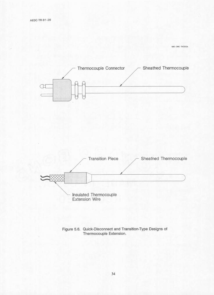
Thermocouplas and their extension wires are usually color coded to aid in identification
and to avoid inadvertent cross wiring. Table 5.2 shows the color codes for the eight most
common thermocouplas.
5.4 Reference Junction Compensation
The EMF output of a thermocouple can be converted to temperature of the measuring
junction only if the reference junction temperature is known and its changes are compensated
for in the measuring circuitry. A simple remedy is to keep the reference junction at a known and
constant temperature medium such as an ice bath (Figure 5.7), or an oven.
In measurement and control instrumentation, maintaining a constant reference junction
temperature is frequently inconvenient. Consequently, some measuring Instruments use a
reference junction compensating resistor (RT) to automatically compensate for the changes in
reference junction temperature (Figure 5.8). The reference junction resistor is at reference
junction temperature and is usually sized so that the EMF from the voltage divider is zero at a
33
AEDC-TR-91-2 6
y Thermocouple C o n n e c t - Sheathed Thermocouple
• Insulated Thermocouple Extension Wire
~ - Transition Piece ~ Sheatned Thermocouple
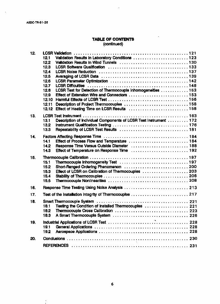
Figure 5.6. Quick-Disconnect and Transition-Type Designs of Thermocouple Extension.
34
AEDC-TR-91-26
E J K N T
TABLE 5.2
Name
Color Codes of Standardized Thermocouples and Extension Wires
Color of Insulation Positive Leg Negative Leg Overall
Base Metal
Chromel/Constantan Imn/Constanten Chromel/Numel Nicrosil/Nisil CopperlConstantan
Purple White Yellow Orange Blue
Red Red Red Red Red
Purple Black Yellow Brown Blue
B R S
Noble Metal
Platinum-Rhodium/Rhodium-Platinum Gray Platinum-Rhodium/Platinum Black Platinum-Rhodium/Platinum Black
Red Red Red
Gray Green Green
35

AEDC-TR-91-26
AMS-DWG THCO43A
: Measuring I Instrument i ~ " - , ~
Leads
• L Ba . , )
+ Wire
- Wire
Reference Junction
Measuring Junction
Figure 5.7. Equipment Setup for Temperature Measurement With a Thermocouple.
36

AEDC-TR-91-26
AMS-DWG THCO42A
I 'o-'t'~meot i I ° l
Copper
Copper
0
EMF
0
Measuring Junction
Figure 5.8. Reference Junction Compensation Circuitry.
3?

AEDC-TR-91-26
reference ambient temperature, ff the reference junction temperature increases, thermocouple
EMF decreases, however, the reference junction resistor increases in resistance, adding an EMF
in sedes with the thermocouple that is equal to the decrease in the thermocouple EMF. The
measuring instrument consequently sees an EMF that is related only to the temperature of the
measuring junction, regardless of a changing ambient temperature.
In digital instruments, compensation for changes in reference junction temperature is
implemented differently. The incremental EMF caused by changes in reference junction
temperature is directly added to or subtracted from the thermocouple EMF. A small constant
current is supplied to the compensating resistor and the variations of the corresponding voltage
is digitized and combined with the thermocouple EMF ~) to account for temperature changes at
the reference junction.
38

AEDC-TR-91-26
6. THERMOCOUPLE CALIBRATION
Industrial thermocouples are not normally calibrated. Rather, they ere used with standard
reference tables or polynomial expressions given in the NBS Monograph 125 or the ASTM
Standard 230. Each thermocouple type has Its own reference table or polynomial expression.
The manufacturers of thermocouple wires end thermocouple sensors usually calibrate
representative samples of the wire after it is made, and apply the calibration to the rest of the wire
or to the thermocouples that are made with the wire.
The standard reference tables are subject to the tolerances shown in Table 6.1. If these
tolerances are not acceptable, then a representative sample of the thermocouple wire or the
thermocouple sensor must be calibrated in a laboratory to provide a better accuracy.
6.1 Calibration Procedure
The calibration of thermocouples may be done by either of two methods: the comparison
method and the fixed-point method. In the comparison method, the EMF of the thermocouple
is measured at a number of temperatures and compared to a calibrated reference sensor such
as a standard platinum resistance thermometer (SPRT), or a standard thermocouple. In the fixed-
point method, the EMF is measured at several established reference conditions such as metal
freezing baths whose temperatures are known from the laws of nature. The fixed points used
for this purpose at the NIST are the freezing point of zinc (419.58°C), silver (961.43°C), and gold
(1064.43°C). in addition, in fixed point calibration of thermocouples, NIST includes a
measurement at 630.74°C. Almost all thermocouple calibrations performed by the NIST and
others are done with the reference junction at ice point (O°C).
39

AEDC-TR-91-26
TABLE 6.1
Typical Temperature Ranges and Representative Tolerances For Standardized Thermocouples
Twe
Tolerance (°C) Temperature Standard Special Range [°C) Grade Grade
Base Metal
E 0 to 900 1.7 or 0.5% 1 or 0.4% J 0 to 750 2.2 or 0.75% 1.1 or 0.4% K 0 to 1250 2.2 or 0.75% 1,1 or 0,4% N 0 to 1250 2.2 or 0.75% 1.1 or 0.4% T 0 to 350 1.0 or 0.75% 0.5 or 0.4%
Noble Metal
B 870 to 1700 0.5% 0.25% R 0 to 1450 ' 1..5 or 0,25% 0,6 or 0.1% S 0 to 1450 1.5 or 0.25% 0.6 or 0.1%
Notes: I. Above tolerances apply to new thermocouple wires in the size range 0.25 to 3 mm in diameter.
Z Above tolerances do not apply below O~C.
3. Above tolerances have a +. sign in all cases.
40
AEDC-TR-91-26
The calibration data are tabulated as EMF versus temperature for the number of different
temperatures in which the thermocouple is calibrated. Each pair of EMF versus temperature data
is referred to as a calibration point. The number and the choice of the calibration points depends
on the type of thermocouple being calibrated, the range of temperatures in which the
thermocouple will be used, and the accuracy requirements. As little as four points are sometimes
adequate, but there is an advantage in taking more calibration points especially if the
thermocouple is to be used over a wide range. The static output of thermocouples is not linear
and their EMF versus te.mperature cannot be modeled exactly for a wide temperature range. The
best that is known to date is that the steady state behavior of commonly used thermocouples
is reasonably represented by polynomial expressions of varying order except for type K. For type
K, an exponential term should be added to the polynomial to provide for a complete
characterization of EMF versus temperature. The general form of a polynomial expression for
the EMF output of a thermocouple (E) versus temperature is written as:
E = a o + a I T + a 2 T 2 + a 3 T 3 + . . . + a n Tn (6.1)
where a o , a I , a 2 , • • • are constants called the coefficients of the polynomial, and n is the order
of the polynomial. An optimum order depends on the thermocouple type and the temperature
range for which the thermocouple is calibrated. Sometimes, more than one polynomial is used
to cover the EMF versus temperature of a thermocouple over its entire operating range. For the
eight most commonly used thermocouples and temperature ranges, the order n has values of
as little as 2 or as large as 14 (Table 6.2).
In preparing the thermocouple for calibration, the measuring junction is usually welded
to the measuring junction of a standard thermocouple, ff welding is not possible, such as when
41

AEDC-TR-91-26
TABLE 6.2
Order of Polynomials for Standardized Thermocouples
Temperature Range (°C) Order (n)
E
K
N
T
Base Metal
-270 to 0 0 to 1000
-210 to 760 760 to 1200
-270 to 0 0 to 1372
-270 to 0 0 to 1300
-270 to 0 0 to 400
13 9
7 5
10 8
14 8
Noble Metal
B
R
S
0 to 1820
-50 to 630.74 1064.43 to 1665
1665 to 1767.6
-50 to 630.74 630.74 to 1064.43
1064.43 to 1665 1665 to 1767.6
8
7 3 3
6 2 3 3
42

AEDC-TR-91-26
an SPRT is used, the junction of the t hermocouple and the tip of the SPRT are attached together
with a wire, or placed adjacent to one another.
Figure 6.1 shows a block diagram of the steps followed by the NIST in calibrating a
thermocouple by the comparison method in a furnace. Bare wire thermocouplas and sheathed
thermocouplas are calibrated the same way. Figure 6.1 shows the process for both the noble
metal and base metal thermocouples. The differences between the calibration processes for the
two groups of thermocouples are that the base metal thermocouplas ere not annealed, and the
calibration data for base metal thermocouples is taken in order of increasing temperatures
specified by the user. In contrast, the noble metal thermocouples are annealed before
calibration, and the calibration process proceeds from high to low temperatures. Instead of
annealing the base metal thermocouples, the NIST requires that new thermocouple wires that can
safely be assumed as homogeneous be sent for calibration.
It should be noted .that a homogeneity test is necessary before a thermocoupte is
calibrated whether it is a noble metal or a base metal thermocouple. A thermocouple that has
any inhomogeneous section may have a different EMF versus temperature relationship when it
is placed in service than it does during the calibration process, depending on the temperature
gradient across the inhomogeneity. It is due to the potential for inhomogeneity that
thermocouples which have been previously heated or installed in a process are not calibrated
without a systematic inspection for inhomogeneity.
NIST also calibrates single leg thermocouple wires. These wires are sometimes referred
to as thermoelements. A single wire is calibrated against the platinum thermoelectric reference
43

AEDC-TR-91-26
AMS-DWG BLKO 13B
Comparison Calibration of Thermocouples (T/Cs) at NIST
Noble Metal T/C S,R,B
I RecmDt I R e VioSula I O ;Er x ° nm~ in°ti° n n~t Conoi(ions} I
I
Bose Metal T/C
I Visual Examinat'on at Rece=pt
(Reject if Not New)
Electrical Anneal 1450"C for 4-5 Minutes
Mount T/C in Insulating Tube Mount T/C in Insulating Tube
I Weld the Test T/C to a
Calibrated Reference T/C
I Weld the Test T/C to o Calibrated Reference T/C
F'urnoce Anneal 1100"C for 30 Minutes
Homogen=ty Check (Immersion Test in o Furnace
at 1100"C). Reonneol or Reject if Not Homogeneous
I Calibrate From 1100"C Down to IOO'C (Measure EMFs of
Test T/C and Reference T/C Simultonlously)
Calibrate (Slowly Increasing Temperature and Measure
EMF.s of Test T,/C and Reference T/C Simultomously)
Figure 6.1. NIST Procedure for Comparison Calibration of Thermocouples.
44
AEDC-TR-91-26
standard identified and maintained by the NIST as Pt-67. Both the noble metal and the base
metal wires are calibrated against Pt-67. The thermoelement is joined with Pt-67 to form a
thermocouple and is calibrated using the process shown in Figure 6.1.
As mentioned earlier, the comparison calibration can be performed with a standard
thermocouple (such as type S), or a standard platinum resistance thermometer (SPRT) as a
reference. When an SPRT is used, the calibrations are performed in stirred liquid baths as
opposed to a furnace (for temperatures above ice point), and the measuring junction of the test
thermocouple is placed adjacent to the tip of the SPRT in the bath, but not attached or welded
to it.
6.2 Processing of Calibration Data
Processing of calibration data generally begins by calculating the difference between the
measured EMFs and the EMFs given In the standard reference tables for the thermocouple being
calibrated (test thermocouple). The differences are calculated for all calibration points and
mathematically fit to a low order polynomial. The coefficients of the low order polynomial are
identified from the fit and summed with the corresponding coefficients in the polynomial given
for the test thermocouple in Monograph 125 or ASTM Standard 230. This will provide a new
polynomial representing the EMF versus temperature relationship of the test thermocouple after
calibration. The procedure is shown in Figure 6.2 and is summarized below:
.
.
Measure the calibration medium's temperature (7") with a reference sensor (a type S thermocouple or an BPRT).
Measure the EMF of the test thermocouple (EM) at temperature 7'.
45

AEDC-TR-91-26
AIdS-DeG BI.,(014A
Data Processing for Corr{porison Calibration
I Measure Bath Temperature
with SPRT or Reference Thermocouple
I Measure EMF of
Test T/C
EMF(T)
I I Calculate the Difference Between the Two EMFs
De = EMF(T) - EMF(S)
I Fit De Data to a Polynomial
I Look up EMFs from
Monooraph 125 for the Type of Test T/C
EMF(S)
I
De = f(t)
Combine the Polynomial w=th Monograph 125 Polynomial for the Some Type Thermocouple
Figure 6.2. Procedure for Processing of Thermocouple Calibration Data.
46
AEDC-TR-91-26
,
.
.
.
.
Look up in the standard reference tab!as, the EMF of the test thermocouple at temperature T, oi use the polynomial expression for the test thermocouple to obtain the EMF (Es):
E s = a o + a 1 T + a 2 T 2. + a s T 3 + • • . + a n T n
Calculate the difference between the measured and the reference table
EMFs; A E = E M - E a
Repeat from step 1 with a different temperature until the differences are identified at all calibration points.
Fit e E to a low order polynomial such as:
AE = b 0 + b I T + b 2 T z + . . .
Identify b o , I:) 1 , b 2 , . . . from the fit. Usually, a low order polynomial such as second or third order is used for the fit of the EMF differences. The decision on the order of the polynomial for fitting the difference may be made by implementing an error minimization algorithm to find the best fit.
Combine Equations 6.2 and 6.3 to obtain the new polynomial for the test thermocouple:
e o= (a o +bo) + (a, + b , ) T + (a 2 + b , ) T Z + a 3 T 3 + . . . + a T"
(6.2)
(6.3)
( 6 . 4 )
An alternative data processing procedure is to fit the raw calibration data for the test
thermocouple to a polynomial directly and select an appropriate order for the polynomial that
gives the best fit. This is a more straightforward procedure that can be implemented on a
calculator or a small computer. The procedure outlined in the 7 steps above is the conventional
approach that was developed to facilitate data reduction when computer data processing was
not as simple as it is now.
It should be pointed out that the discussions that we have carried in this chapter do not
reflect the new International Temperature Scale of 1990 (ITS 90). The new scale became effective
on January 1, 1990. In light of the ITS 90, new guidelines may be applicable to the calibration
of thermocouples.
47
AEDC-TR-91-26
7. PRINCIPLES OF THERMOELECTRIC THERMOMETRY
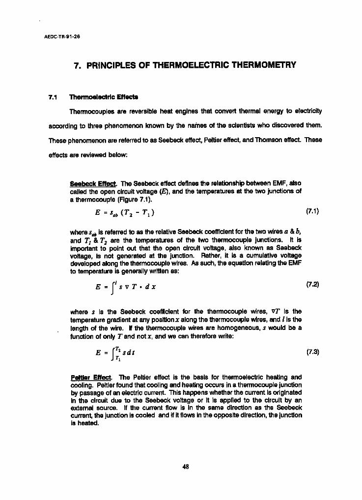
7.1 Thermoelectric Effects
Thermocouples are reversible heat engines that convert thermal energy to electricity
according to three phenomenon known by the names of the scientists who discovered them.
These phenomenon are referred to as Sesbeck effect, Peltier effect, and Thomson effect. These
effects are reviewed below:
Seebeck Effect. The Sesbeck effect defines the relationship between EMF, also called the open circuit voltage (E), and the temperatures at the two junctions of a thermocouple (Figure 7.1).
E = Sob ( T 2 - T 1 )
where s~, is referred to as the relative Sesbeck coefficient for the two wires a & b, and T l & T 2 are the temperatures of the two thermocouple junctions. It is important to point out that the open circuit voltage, also known as Sesbeck voltage, is not generated at the junction. Rather, it is a cumulative voltage developed along the thermocouple wires. As such, the equation relating the EMF to temperature is generally written as:
E = f t s v T . d x
(7.1)
(7.2)
where s is the Sesbeck coefficient for the thermocouple wires, vT is the temperature gradient at any position x along the thermocouple wires, and I is the length of the wire. if the thermocouple wires are homogeneous, s would be a function of only T and not x, and we can therefore write:
E = " I ~2 s d t J T1
(7.3)
Peltler Effect. The Peltier effect is the basis for thermoelectric heating and cooling. Peltier found that cooling and heating occurs in a thermocouple junction by passage of an electric current. This happens whether the current is originated in the circuit due to the Sesbeck voltage or it is applied to the circuit by an external source. If the current flow is in the same direction as the Seebeck current, the junction is cooled and if it flows in the opposite direction, the junction is heated.
48

AEDC-TR-91-26
AMS-DWG THCO46A
i l ,'~it
T1
E
T2
11
Reference Junction
T2
Hot Junction
Figure 7.1. Typical Thermocoupie Circuits.
49

AEDC-TR-91-26
The Peltler effect is not related to thermoelectric thermometry, but it has an implication in the response time testing of thermocouplas using the Loop Current Step Response (LCSR) method described later in this report. If a DC current is used in performing the LCSR test, then the thermocouple may undergo cooling or heating, depending on the direction of the applied DC current. Initially, this effect was thought to be detrimental to the LCSR test if it cooled the junction, and subsequently it was thought to be helpful to the LCSR test if it heated the junction. However, laboratory tests performed in this project have shown that the Peltier effect is neither signIficantly harmful nor significantly helpful in testing the thermocouple types and sizes studied here. Nevertheless, in the LCSR developments which were carried out in this project, high frequency AC currents were employed to avoid the Peltler question altogether.
Thomson Effect. The Thomson effect occurs in a single conductor as demonstrated in.Figure 7.2. If a conductor is heated at a point to a temperature T z, two points PI and P2, on either side will be at a lower temperature T 2 . If a current flows in the wire as shown in Figure 7.2, electrons absorb energy at point P2, as the current flows opposite to the temperature gradient, and release this energy at pointp z, as the current flows in the same direction as the temperature gradient. Because the gain and the loss are equal, there is no net effect along the wire. That is, the application of heat to a single homogeneous wire does not generate a net thermoelectric voltage according to Thomson (Thomson is also known as Lord Kelvin).
Although the behavior of a thermocouple can be described in terms of the simple
relationships such as Equation 7.1, it Is not simple to model a thermocouple to predict its output
analytically from information about its structure or composition. The EMF versus temperature
relationships of thermocouples are predominantly empirical, even though thermodynamic
principles and free electron theory of metals can help provide a qualitative insight into their theory
of operation.
7.2 The Laws of Thermoelectrlcity
The behavior of thermocouple circuits has been summarized in terms of statements
referred to as the laws of thermoelectdcity. There are about six laws, three of which are the most
important and useful and are discussed below.
50

~..,;< :i. 4:-' , i (,..~'-:' :~.: " - -~= - . - . , , r . c i . g
. . . : ~.---.~:.,.~,:,~:~: ~,.;?~:-": .:::,,
. . . . . ~ . . . . ~ I ~ I t l y I " ~ . . . . . . . I I ' : : I " ~ : ; I : I I i I " ~ J . 2 I I " : ' I * " " i ' I ~ ' i~J; " I ; ~ ~ "~ I i ~ " I ' ~ "
"! : i . : . ! "~:~ , ':::',.: :;,~. ~ ; .~ " " - ~ ; , ,~ : - " " ' 7 ~ ~" -'. ~ ,:/.- ~ : ~ ~ ..~ _ . = ) • ,. , :. , . , j . . . ; ' - ~ , : . , _:c" . ". , ~ ! -::,,; : , I :~ • Z t : ~ - - ~ d ' : ~ -~: :,:" -" ' , . . . . , : ~ , - ; , : . , - ~ , ~-t , ~ . : % , u ' . , , , , ~ . :~ . . ~.
, . ~ - ' j ,,~_ ~ ' "" " ",,, £ " , , i - ' . ; . ' t ? . ; - ~ 7 ' - : " ~ ; . . . . . . . ' ~" . . - ::X ' ~ ' ' . ~ , . t , 9 " • ~ , " , ,~ '~ " " :*~ ( . . ' : , • . ' £ , : ~ : ~" '.;:.~ : ~:,~<.~ - ' . . - ' , ' ,
. . . . , ~ - ~ , ~ ~ , , S , / : ; . , .-
' ;~ :K' .:~: I . , L " . : : , : :~ " : % , ; ~ ; ~ " . ~ : ' ~ "";" ' : ~ .~:..-':-' . :7 / : ,:.~_E~ ,.-. : , : ' : . . - : - . , : !, :~:, ~. : ~ . . . . . ,_.:,: ~ f : . ! ! ," '": . , . '~: . ' ~ . . . . ~ . : ' ~ " . . . ,.~,~-~.. , : . - -- , : ' ; - . r .~.::!': J ; .k ::.,..: ,.: .%f/'!t.,.;; ft,L!.. ,:- ': ,....;'~. ' " ='.V" : .'T "' ~: ~,"";.,"" ' ~ % -¢'" , - , .-: - ~'~,~'5-" ~. " -- ' ;.:f: -.'.:J :...<g - ,
:/,:;~; :~ :- .~P,; ~, ,:, ~, ~',., ~..-'~-., ~ . ~?-;,.-~: ':~.~K ' :,'--k~;.-~ . '..:~,~ i~ ~..;;~.;/," ~ :. -,~..!~-..i',~~ ~ * ,, ..~ .4/?, ¢.~,:~. ~,,.: ,;:_- :: .,- ,~ • i:: ,:,'., :'., .,. , .,~:~ :.~, - ;" .. • =* , , ~ ; ' , , ' ~ , , . ' ...,~ . . t ~,,.: . * : ~ ' . ' ~ " . : ~ .~>.:1~'>' " - , ~ . ' ~ - ' ~ , ~ " ' . ~ . . . . " ~ , t , d . , * , + " ; ~ . ~ , - T ~ J ": ' : l ~ : ~ ' ~ ' . ~ t . ~ ~ ! ' ~ . - - . . , ! ": ,~-~. , ~ . - ' . ; ' - • * '" / - " ' . " L: . J , l ' ~
; ' : " -:-' " '" " ; : U ? : - ~ - ~ ' " - ( ~ , ~ ' , ' ~ . ; . . . . ~ , ~ t : 4 { / ~ , ! " " : . ' ~ ~ - } ' ~ - ~ D ~ ( , : ~ - - , ' ~ K - . . : . - : . ' ~ . - . ~ : p . 7.: r . ~ A ' . ' [ . / ' , ~ 1 , . ~ : . . , ~ . ~ : ','~1~- ..
- " . ' . ~ ~ G ; " : . t ! : , : ~ : . . . ; ~ , - ' ~ . ~ . : i ' ~ . ~ i ' - : ~ ~ --' , ~ > " * < L k , " - . - t ' : . . : : " : - " ; : ~ - ' , ... ; - : , - - ; , ! : : . , f : ;~ ,*,~>~.:'~.~ ~ , ' : ~.. 7': .,- .,"
. ~ : ~ ' . 7 < ~ . ' : ' ' ' ~ ' ~ . ~ : ' ' ~ " " ' - ' " " . . ~ = - . ' - ~ ' . : : : ' . + : . , " . . ~ - - ; " " ~ , " ~ " ' - . , . .,.- ";~.~ " ' : r ' ~ : ; ' ~ : . ~ : . , " ~ . - " . , ' - ~ , ; ' : . . . . " . ' ' : ' . " ' : ~ ' . , ' ~ , . ' . . ' .: • :_' = ~ , ' ~, .~,
. : , . . . . . . . . . . . - . ~ , : . ~ , .~ - . . , . . . . . . . ' . ~ , . ~ , ~ . , , , . . . . ~ >, , ~ , . , ~ . - , . ~ . . ~ : . ~ , . - ~ , . ~ . . , , . ~ . .:.~ . ~ . ~ .
~ , ~ .._ r . . . . . . . ~ ' . . . . / . . . .
' " :'::'~'.r ' ~ ' ........ ;: ,: : . ; " ' " " " } . : : , ,~ . . : Y ' . , . . ..:!;: ;
'":; : : , ~ " . - . - . ~ ' 2 - . , " . + ~ ~ ; , l * ' ! , ~ , ~ ' : r . , - , , ~ ' , - , ~ , :u " + : " , , ' ~ ' 7 C , ," - , : = , - h ~ ' ~ ' ' ~ . , + -,' ~ - . ~ . , , ' . , ' : ~ . : ; . : t , . . , , . . . . • ~ ~ . " , , "
' " ' " ' ~ ' : " C : I Y " ~ . ' : - . < ' i * ' c = .-:. .... .: * :)' ,,. . . . . . , ~ . ~ ~ . . , . ~_; . ~ . . ~ . , . , u ~.:~ . r " - ,- "~ '~ t ~ i
; . ~ : d , " ~ ' : . . . . " . . . . . . . . ~ . . . . ~ . . . . . . . . . . . . . ~ , ~ ' . , , , " ] ; . i ~ , ,:- , ~ , i -~"~", ' l : .~ ~ , , ~ r : " . ,~! ' .~ ' " t , ,~ ,',,'::"~:.:~'~,
1 ~" - ." ! [I~_ 7 ; I " ~
) ' u ~ . . . . . . " ' : < " : 7 'oA
' ; i ' , ' " . ' - = - ~ ; -L ~[I . - , r ' ' , 'r" = : ' 7 j " . ~ " , , t , ' ) Y ~ • " t ' " " ' ' ' , ; ~ r , " , : ' . ~ ? • . . . ' . . . ~ , , - . : t :~" , L " r " " ; - - - "
":" " ~ : P ; - ~ : ' I " . ' ~ ' ~ :~' 2 ~ ' ' ' ~ , ~ :~:("bt~t"~l~.~-;•~:"•ti~,,'~/;~*',~.: " '~ . " ' } ' ' ~ " ' ~ : ¢ : - * " ' ' ~ = " : ' " ~ L ~ t ' . ~ ' ~ , ' ' ~ d ~ - ' ~ : ' ~ , ' : ' , " ~ " ' . " ~ . ~ ' - ¼ ~
: : ' : ; " ' . 1 ! , ~ . ~ : ' " , * " ' . . . . . . . ~ - . r ~ ; : , . ? ! : ; , . ~ p , ~ • / , . . ~ . t 2 , ' i . ! . ~ L ~ i ; ' . , . ; ' , [ ; ; i ¢ ' f " - ~ : , , T ' ~ , ~ . " ! - . \ : ~ 1 [ - , ! , ~ , . ) . . . . . ~ ! . ~ : = ~ f , } ' - , , I . . . ' , . r ' . i . ~ . 1 ' . . ' ,' ' t * ' ~" , , " t ' , ] , ; ' ~ , ! - , " ~ ' ; ' . , , ; , : , " " . ; - " , . , '4 * , ' ; : . . . . . ' . ; . : : ,~: " : -;" , ; " " " ~ ' , ~ ~ ; ' ; ' . - : . , 7, : : , ~ . , . ~ . , . , " . - . ' . ,: . . , ." , . ~" , . ~ . . . . _ -
Pit111 I I I " I " ~i" " ~ " l I t " " ' , ) * [ ~ "~ I ' = { [ ) ~= ' = -- P ~ ~== '~ " [ " * i ~ " r . l ! P i r t I ' . ~ ~ : : L " I = I . ' I 1" ? [ r " i ~ ' [ : I m I " ~ - - " ' ~ . ' ~ l l ~ ' ~ ~J I I : I i
. . . . . . . . . ~ . . . . . . . . . . . . . . ~ , ~ , . . , . , , . : ~ . . . . . . . ~ • . _ . ~ , ; . ~ , , , . : . ~ . ~ , .~ . ~ . . ~ ~ - . . . . . . ~ , : . , . . . . . . .
"¢" ~ " . . . . . . . ~ . . . . . [ ' ~ " ' ~ " ' t ~ ¢ - ' - ' - . . . . . . . " " " " ~ ' , ¢ " ~ ' ~ o " " - = . . . . .
= ~ " " ' " "'~'~ " =-' - ~" L ~- Ir'~. . .. i. -I ~-.. - . . . . ,= .. ~, ~ - . ~ '~; • ,--~- -~" . . . . . .
~ ' J " ; . I " . ~ . . I I " i I : . . . . . I ¢ i i - ~ ; I ; ~ , II * I : I J ~ . . d I I " , I : I " . . . . . I I " , r I " I : I I . ' ~ 'l I • . I . . . . . . . . ~ ' ~ ~ . " ~ = " . ~ : t . I : : J~:'
• "-- , , ~ , • '-~ "" ~ ~- ' : . . . . ~ " . - ~ ' " , . ' ~.~ ~; ' - - . ~ ' 7 - • -= ~ - 7 ~ ¢ ~"
~ " ~ ' ; ' " ~ ' ~ " '~ ; ~ ' " ~ ' " ~ ' ~ " " ~ " ; " : "~ ' . . . . . . " ~ ~ " " . . 7 . : '
• ' ~ = : : r " ' , , . ' '- - ' " r : ' . ~ ' , - ~ ~ . - " ~ , . ~ " : 7 -./.I" d : ' i ' . , :;'~r:,':. ' . . ~ . . . . : . . , ~ . . . . ~ , . ; , ; . . . - ; ~ - . _/,,. : - , ,' , . U . . ~ ! A ;,
.... " " ~ ' :'-';'- . . . . . . . . . ' : '~ ": ..... ,' . . . . . . . . '.!:' ~ -i~;i.:~, ' " " ~ '~
. . . . . ~ '~ " " " . . . . . " . ' = ;~ '" " ' ~ : . ; ~ ' - ' i : . ; ' l~ . . ; : .~' I r a : - . ~ : . , ~ , ~ ~ ' . . . . . . . . : ~ ~ . . , ; " - : - . . ; ' . ' . ' : ' := ' 2 ~ , ~ ' - , = ' r * ' ' ' 1 ~ ' 7 / .
.r.'- ~,~i. ' " i ! -~ ' - , . . ' !i. '-- , : . = :: ';
" :':t ~:." ' / " ~ " - t ' ~ ' '~ :i ~ :: ;': ;:': ":~: ~ * : " : " ~ , ~ t : : ' - ~ 7 ; ! , [ , - ~ . - . ; ~ ' . . :~ .
' " . - - - , , • ~ , : . , . - . - " , , - . - : " ~ . . . . . , , ~ . . . . . ~: .~ - . , ' ~ . . , , , : ' ~ . . I < ~ t r ~ ' ~ . ~ , , . . . . , , . . ,_~ - , , . . , . , . . ~ , . , ~ . . , . , , ~ . , , , W ~ -~, : ' ; ~ " " : i t ~ " l ' r m N' i . ' I I ~ I . ; " ~ " ~ " ' ~ i . . . . " ~ " j ~
:: . . . . ~.: ~ :,,::~, !. ~ . . " : * : . . 7"., ' ,,.. "
, - . 7~:-' ,~ , : - - , - ~ - , , . ." .~," , ¢ . ' d : - , . - . , , - ~ .
~ ' . ~ [ ~ : , ,. - , , . .: . .~ . , . , . ~ ,~ ' : . .~: ; " '~ . .~ . . . . : . - ..~ ,.- : , . - , . . . . : . . ~, r ' , .
. . ~ - - . . . ' - ' t " ' ' - " . . . . - -~ - . ~ . ~ ~ ~ ' , . . ~ , ~ ' - '>~ ~.~ " { ~ . . ~ : t ~ , s ~ ~ , ' ~ " ~ . ' ~ - ; . " ' / ~ - : . . . . . . ; - ,. ' ~ ' , ". ' ~ - ' . " " : r
" : " " " I I " r . ~ ' I I I " " ' I I . C " : ) ~ ~ I 111 " I . I I ~ I I ~11 11 - - I i . I ( . I ' " " ] ~ * I ~ " ~ ~ ~ ' " ~ ~ " j I. I ~ " ; " I-- J J~
~;..?~," . . . : ' . . : ~ . : ~ : ; . ~ i ~ , . , . i ' ;# , , :~ , .~ . . / . - , . ,- . . ; . . ~ . ~ .~ , , - . ; ~ : , , . ~ . ~ , _ . . , , : - ~ , i ~ . . } . L ' : . : . .~ . '~ • ~ ' ~ ' , ' - ~ :- > ' : ; v ; : , . L ~ - ~ : 1 ~- ~,,- ,~ , - . ~ " ~ p ~ . . ~. r L ~ . " ~ ' , ~ . . . . ' , ~ " ~ . : ' ~ ' * 4 , I , " _ o ~ . ~ " L " ~ ' ~ . • ; - , ,~ r }! . . . . ~,: ' ,~ -: ~ . " . : ~ ." ~ ; " - ' . ~ , 4 " * ' ' , ' ," . • ,~,t" . , , . ~ " " . . . . / ' " , - - ~ .~, I . ) ~ [ ' " 1 1 y i l l ' I " i ¢ ' " I ~ I I : I - - I : I ) i : ~ I " : ~ I I [ ' I I " " ~ . I I I " : ~ ~ : # ' ' I : I ~ = " I ' ' ~ r . . . . . : ~ :~ : I: : ' I I . L Y ' . ~ I
. . . . . ~ . . . . . . . ~ , - r ~ ' ~ - ~ ~ ' : ~ ' ~ ' • ~ . . ; , , ~ t , ' ~ ~; ,~e . . . . . . . . . . . . . - ' . ~ ~ - " ~ " " . - . . . . . . . . . . . . , / . . . . ~ : • G : : . : . ' , ~ , , ~ , = . ' : .... ~ . . . . . . ~ ' . . ~ , ; . - . ' , - ~ . . . : ' : ' , " . , ' . : ~ " :P r ' - ! - ' / . - - - ~ ' ~ " - " P r . ' - ' ." • ' ~ " ~ , ' ~ " ' ~ ' " ~' k " ~ " ' ' ~ ' ~ , ' ^ '~ ~ "' - ' " ~ ' : '
, . .~ ~ : , . , ' 7 ~ ~ . ~ . ; ~ , , ~ - ~ . b . ' t ~ ; f " < . . ' . ' ~ . . . ' , ~ ' " -~' . , ~ . -'"'~ , ;~:'~: ; ; . , ~ ' ~ ; ~ ~ . , . ' " - : : , : , ' ~ , ' : ' " . . . ' ~ " ' '. " .. - ' : - ' . . ' ] "" ' - . , ~ • . " ( ~ .: . < : . ~ - -. ' - ' ' - • . ' " -
~,:.::r ' .: :-, . , ." ~ . C ~ " ' " . - ~ : . ' ' ~ ' i , ~ " i , , * ~:-:~ . ~ . ' ; ' . - ~ ~. . " . " ' ~i ,~ ~ : " - . ~ . ; - ~ ~ h:::! ' ~ " " . : ~ : " " . ~ . ' i ~ : : ~ "~2' ~ . - . . . ' : " t ' ' ' ~ , ' : , - ; , : : ~ . , ~ : ~ . t : ' : ; ~ ' ; . i : ! . ~ , , " . - , ~ , 2 : : - , 4"°?':':
" . : ' ; '111 "~ " , i = : I " S ' ~ ~ ' . ~y : : [ : ~ . r " - J~ ~ ; ~ " i ~ J ~ I I ~ I ~ [ :I: ' I~ * : ~ 1 . . . . . I* [ . : 1 . , I [ - .[ I I : Y ~ " . i I ~ ~ , I

AEDC-TR-91-26
.
.
.
Law of Homogeneous Metals. The EMF output of a thsrmocouple made of two homogeneous metals is not affected by temperature other than the temperatures at the two junctions.
Law of Intermedlete Metals. In a circuit of dissimilar metals, if a third homogeneous wire is added between points X and Y, as shown in Figure 7.3, no additional EMF will be generated if points X and Y are at the same temperature. Stated differently, the algebraic sum of the EMFs in a circuit of any number of dissimilar metals is zero if all the wires are at a uniform temperature, i.e,
N
E M F = s, ( T , . , - T,.) i ° 1
A special case of the law of intermediate metals is described below:
If metal C is inserted between metals A and B, at one of the junctions, the temperature of C st any point away from AC and BC junctions is immaterial as long as the junction AC and BC are at the same temperature (Figure 7.4). This law indicates that the measuring junction can be formed by any number of ways such as a wire made of any material, soft solder, silver solder, brazing, or wrapping the metals together and/or welding as long as the thermoelements of the measuring junction are connected electrically.
Law of Intermedlete Temperatures. The EMF generated by a thermocoupla between temperatures T A and T c is the sum of the EMF generated (by the same thermocouple) between T A and 7' 8 and that generated between T B and T c if T A < T B < T c. This is the basis for using the generic thsrmocouple calibration charts that are written with reference to 0°C.
('7.4)
7.3 Thermocouple Circuit Analysis
A few examples of typical thermocouple circuits are discussed below to illustrate how the
three laws of thermoelectricity are used and to help In diagnosis of thermocoupls circuit
problems.
Example 1. Recalling that the sum of individual Seebeck voltages in a thermocouple circuit equals to the tharmocouple output EMF, we start with the simplest thermocouple circuit (Figure 7.5a):
52

AEDC-TR-91-26
AMS-DWG THCO54A
Metal A Metal B Metal C Metal
I X Y j
~--Isothermal Connection
A Metal C
Figure 7,3. Law of Intermediate Metals.
53

AEDC-TR-91-26
AMS-DWG THC070C
~ . : v ._. v.. : . _ . . , : . ~ - . v : _ ._...:. :_ _ .v.., : .
:i<i< :! d= ~ ::¸::¸::¸: : ¸̧ -< .7 . - IY . [< : . I -h , , .<bY
>b i - , i i ,<i i i . i . i i I Y i i i i i
~i~ii i i i • i i i • ~ b i i • < •k •~
iiii iii~i ~i ii i I ii•ii[i•i : i i I i I i l l i
iii I i~iiiii i i 71~<~iii •11•711 iii i ii
k l l ~i: i• i<• i r a , • i i • i<< +
• • , • • ~ < iiiii I~IY v < , - • . . . . . . - • • • ' • : :
<•X•bi i i i~, i l i i i i i Y•~
C
J
::i !iii!i !iii!i!i ! ¸ i !i!i! !ii!: i! ii i i l b lb l , ) i i ' i k , i i i [ i
iiiiii i iii iiiii i I ~i i I ii~i ~i~ii~iiiiii~i ~iii~i i i
!ii!ii!iiiiiiiii!iiii!i:i iii I ill i!
Y.YC < >i Y , Y . b l b I Y ' Y I >7<,i. i>>bi l , i . b Y C Y <
• :. • : , . • . . . . . .
>XC<< b b ~ i l ~ I I Y < i i . v : . . : - : . : ; . . . . "
To 71
Figure 7.4. Special Case of Laws of Intermediate Metals.
54

AEOC-TR-91-26
0 / . . . . •
S 8
Sb ~ T2 (a)
To S c r . . . . • i
G I To S¢ t . . . . . •
T1 Sa
1" 1 S b (b)
r . . . . •
i I
Q i
, T O S b / . . . . •
T1 Sa I
T1 Sb I
(c)
T1 Sa T2 I \ I
, sa!Ta TI S b _ J
T2 (d)
Figure 7.5. Thermocouple Circuit Analysis.
55

AEOC-TR-91-26
E = s . (T~ - T~) . ~ CT, - T~)
= so (T , - 71) - s , CZ'2 - T1) = (~. - s , ) (T , - T~) (7.5)
where E is. the open circuit voltage of the thermocouple, T l & T 2 are the " temperatures of the two thermocouple junctions, and s a & s b a r e the absolute Seebeck coefficients for the two thermocouple wires, If the relative Seebeck coefficient in denoted as s,a,, we can write:
s,, - s b = s ~
E =S ,b ( T , - T~) (7.6)
Example 2. We now show the effect of extension wires on the output of a thermocouple (Figure 7.5b). Assuming that the extension wlras are made of copper with Seebeck coefficient s c, we can write:
E = ,~ (T~ - To) +~o (T 2 - Tt) +s~ (T~ - Tz)
+ so ( T o - TI) = s.~ (T~ - T~) (7.7)
That is, the addition of the extension wires does not alter the thermocouple output.
Example 3. Sometimas thermocouples are extended with thermocouple extension wires made of similar materials so that the reference junction can be placed remote from the thermocouple site. Assuming that the extension wires have Seebeck coefficients s" and s~ (Figure 7.5c) we can write:
= ~g (:r~ - To) + ~, (T, . - : r~) + ~ ( : r x - :r~)
(7.8)
t
E = s o , , ( r ~ - T o ) if ~ , = ~ .
Note that the temperature T z (which occurs at {he thermocouple connector site) does not have any effect in the output as long as s;, b -- ;=~. Note also that it is not required for the absolute Seebeck coefficients to be equal as long as the relative Seebeck coefficients are equal (s'-b = s,~).
56

AEDC-TR-91-26
Example 4. This example corresponds to the law of thermoelactricity which allows for the junction to be made of a third material such as soft solder, silver solder, etc. If the Seabeck coefficient of the third matedal is s d, we can write (Figure 7.5d):
E -- sa (T2 - T1) + Sd ( T 3 - 72) + Sd (T2 -T3)
÷ Sb C7"~ - T ~ ) =s°~ CT,. - T t ) (7.9)
A consequence of the above analysis is in cases where thermocouple wires are individually attached to a metallic object to measure its temperature. This analysis shows that the thermoelectric properties of the metallic object play no role in the temperature measurement.
57

AEDC-TR-91-26
8. FUNDAMENTALS OF SENSOR DYNAMICS
The dynamic response of a sensor or a system may be identified theoretically or
experimentally. For a temperature sensor such as a thermocouple, the theoretical .approach
requires a thorough knowledge of properties of the sensor internal materials and their geometries i i = ~ "
of the properties of the medium surrounding the ser, B~)r ~. :Since these 8S well as a knowledge
properties are not known thoroughly, or may change under process operating or aging
conditions, the analytical approach alone can only provide approximate results. A remedy is to
combine the theory with experiments.
The theory is used to determine the expected behavior of the sensor in terms of an
equation called the "model" which relates the input and the output of the system. The system
is then given an experimental input signal and its output is measured and matched with the
model. That is, the coefficients of the model are changed Iteratively until the model matches the
data within a predetermined convergence criterion. This process is carried out on a digital
computer and is referred to as ~ t~# ' . Once the fitting is successfully completed; the coefficients
of the model are identified and used to determine the response time of the sensor. However, if
the sensor can be represented with a first order model, a fitting is not necessary because the
response time can be determined directly from the output of the sensor, The definition of a first
order model and Rs dynamic response Is described later in this chapter.
The model for a sensor or a system may be expressed in terms of a time domain or a
frequency domain equation. The time domain model is usually a specific relationship giving the
transient output of the system for a given input signal such as a step or a ramp signal. The
58

AEDC-TR-91-26
frequency domain model is often represented as a general relationship called the "transfer
function" which includes the input. If the transfer function is known, the system response can
be obtained for any input. As such, the transfer function is often used in analysis of system
dynamics.
In steady state analysis, the transfer function is a constant called "Gain" which relates the
DC output to the DC input (Figure 8.1). The Gain is also referred to as the zero order transfer
function. In dynamic system analysis, the transfer function is defined in terms of the Laplace
transforms of changes that occur in system output per changes in system input (Figure 8.2):
G (s) - 6 0 ( s ) (8.1) 1(s)
00 = ~I =
$ =
transfer function changes in system output changes in system input frequency domain parameter
The section that follows uses a simple example to illustrate how the transfer function of
a thermal system is derived and how it is used to interpret experimental results.
8.1 Response of a Simple Thermal System
Consider e thermocouple whose sensing section is assumed to be made of a
homogeneous material represented by the mass "m" and specific heat capacity "c" as shown in
Figure 8.3. The response time of this system, when it is suddenly exposed to a medium with
temperature T:, may be derived theoretically using the energy balance equation describing the
59

AEDC-TR-91-26
AMS-DWG PXTO 14P
<: '1 <~ I
T Ka
Time Time
Input G
Output r
Ka G = m a
Figure 8.1. Illustration of Zero Order Transfer Function.
60

AEDC-TR-91-26
AMS-DWG PXT014 (
Input ~1
i==,..._ v
Transfer Function
G Output <~
v
Figure 8.2. General Representation of Dynamic Transfer Function.
61
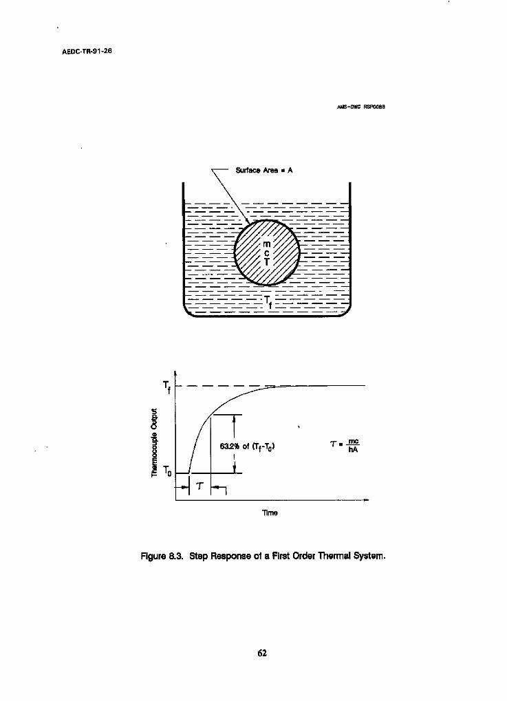
AEDC-TR-91-26
~S-DWC RSP008B
Surface Area = A
: i _ _
i ~To
/ / - , . J T
6~2, of (Tf-T 0) !
i
~__rnc hA
"rime
Figure 8.3. Step Response of a First Order Thermal System.
6 2

AEDC-TR-91-26
system.
write:
Assuming that the thermal conductivity of the thermocouple material is infinite, we can
d T ffi h A ( T I _ T ) (8.2)
Equation 8.2 is a first order differential equation representing the dynamics of the first order
thermal model, and its parameters are:
h = heat transfer coefficient A = affected.surface area T = response of the system as a function of time, t.
Equation 8.2 may be solved in time domain by integration, or in frequency domain by
Laplace transformation of both sides of the equation. We will proceed with the latter approach.
This will allow us to express the solution in terms of a transfer function of the following from
which relates the Laplace transform of the output, T(s), to the Laplace transform of the input,
G(s)- T(s) (8.3) TICs)
The Laplace transformation of Equation 8.1 is:
where
sT(s) - T(O) = p [ T f ( s ) - T(s)] (a.4)
hA p = m c
s = Laplace transform variable
To simplify our derivation, let's assume that T(0) = 0 , then:
63
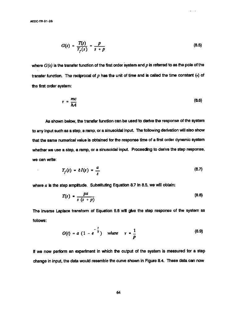
AEDC-TR-91-26
G ( s ) = .T(s) _ p (8.5) T:(~) ~ + p
where G(s) is the transfer function of the first order system and p is referred to as the pole of the
transfer function. The reciprocal of p has the unit of time and is called the time constant (r) of
the first order system:
m c (8.8) hA
As shown below, the transfer function can be used to derive the response of the system
to any input such as a step, a ramp, or a sinusoidai input. The following derivation will also show
that the same numerical value is obtained for the response time of a first order dynamic system
whether we use a step, a ramp, or a sinusoidal input. Proceeding to derive the step response,
we can write:
a : _ = ~ l ( s ) (8.7)
$
where a is the step amplitude. SubstRuting Equation 8.7 in 8.5, we will obtain:
T(s ) - pa (8.8) s (s + p)
The inverse Laplace transform of Equation 8.8 will give the step response of the system as
follows:
t - - ] (8.9)
O(t) = a (I - e ") where T = -
P
If we now perform an experiment in which the output of the system is measured for a step
change in input, the data would resemble the curve shown in Figure 8.4. These data can now
64

AEDC-TR-91-26
AMS-DWG RSPOO1F
0 C~
Ib--
0 r -
CO
Time
a
Figure 8.4. Step Response of a First Order System.
65

AEDC-TR-91-26
be fitted to Equation 8.9 to obtain the time constant (~). However, fitting is not necessary in this
simple case because Equation 8.9 can simply be solved for t = ~- as:
O(t = T) =a(1 -e -I) = 0.632a
O(t = ®) = a ; a = .final value (8.to)
Equation 8.10 shows that the time constant of the system can be identified directly from
the transient data shown in Figure 8.5. This is done by determining the time that is required for
the system output to reach 63.2 percent of its final value.
r The ramp response is obtained by substituting the Laplace transform of a ramp signal s-. ~
for T/ (s) in Equation 8.5:
T(s) - rp (8.11) sz (s * p)
where rp is a constant which we denote as k. An inverse Laplace trarisform of this equation
results in:
-' (8.12) o(t) = k [t - T * Te ~]
A plot of this equation is shown in Figure 8.6. Note that when t> > T, the exponential term will
be negligible and we can write:
O ( t ) = k (t - T) (8.13)
That is, the asymptotic response of the system is delayed with respect to the input by a value
equal to the step response time constant (7-).
66

AEDC-TR-91-26
AMS-DWG PXTO25E
2~ of a
I - ~ T ~ Time
a
Figure 8.5. Determination of ~me Constant from Step Response of • First Order System.
67

AEDC-TR-91-26
AMS-DWG PXTO22E
co E O CL cO
r r
Input
"T
Output
Response Time
Time
Figure 8.6. Illustration of Ramp Response.
68

AEDC-TR-91-26
For a sinusoldal input, the response time is expressed in terms of the reciprocal of the
corner frequency of the frequency response plot (i.e., the break frequency of the Gain portion
of the Bode plot). The comer frequency is denoted by the letter ~o. We will show that ( 1 ) is ¢0
equal to the time constant (T) for a first order system. Substituting j~ for $ in Equation 8.5 and
writing ~- for (-]), we will obtain: P
G(j=) - . ] (8.14) ]~0T + 1
where ~ is the angular velocity in radians per second and j = ~ , a complex number. The
magnitude of G(j~) is:
IGI
The corner frequency is the frequency at which I G I = 0. 707.
1 above equation and solving for T, we obtain T = m .
¢0
(e.15)
Substituting this in the
8.2 Charecterlatica of First Order Systems
A first order system is defined as a system that can be represented by a first order
differential equation such as Equation 8.2. A first order system is also defined as a system that
has only one pole in its transfer function such as Equation 8.5.
The response time of a first order system is expressed in terms of an index called time
constant, ramp time delay, or frequency response, depending on how the index is measured.
69

AEDC-TR-91-26
If it is measured using a step input signal, the response time is usually expressed as time
constant. If It is measured using a ramp input signal, it is called a ramp time delay; and if it is
measured using a periodic signal such as a alnewave, it is celled the frequency response of the
first order system. A unique feature of a first order system is that its time constant, ramp time
delay, and frequency response (expressed in terms of reciprocal of corner frequency), are
numerically equal. Figure 8.7 presents a summary of the dynamic responses of a first order
system for four different input signals. This includes the response for a nondeterminiatic input
signal such as the random noise shown in the last item of Figure 8.7.
8.3 Definition of Time Constant
The time constant of a system in general is defined as the time required for the system
output to reach 63.2 percent of its final value following a step change in input. Although this
definition is based on the response of a first order system (Equation 8.10), It is conventionally
used in defining the response time of temperature sensors such as thermocouples and RTDs that
are not necessarily first order.
NI references to the term time constant throughout this report correspond to the definItion
given above, regardless of the dynamic order of the system.
It should be noted that the normalized step response transients for two first order systems
that have the same time constant are readily superimposed, while the step response transients
for two higher order systems that pass the 63.2 percent mark at the same time may or may not
have the same transient behavior (Figure 8.8). This indicates that a single t~me constant does
not adequately characterize the dynamic response of systems that are not first order.
"70

AEDC-TR-91-26
Summary AMS-DWG PXT087C
Input Output Result
J
~ ~-- Output
TTme
i
Fb Frequency
Fu Frequency
Tu~o Conslanl
Ramp Time Delay
FrecrJecmy Response
1 3 - - -
2 ~ F b
Response Time
7- - 2 ~
Figure 8.7. Transient Responses of a First Order System for Various Input Signals.
71

AEDC-TR-91-26
AkaS-DWG RSPGOgA
1.000
0.632
t:
3"
Time
Figure 8.8. Possible Responses of Systems Higher than First Order.
72

AEDC-TR-91-26
8.4 Response of Higher Order Systems
Although some systems such as the simple thermal system discussed in Section 8.1 can
be approximated with a first order model, the transient behavior of most systems is generally
written in terms of higher order models. This includes thermocouples which should generally be
represented by the following transfer function:
G ( s ) - T(s) _ 1 (8 .16)
~(s) (s-p1) (s-p2)... (s-p.)
Wherepl, P z , • • . , P , , are called the poles of the system transfer function. The poles are also
referred to as the modes of the system's response. The reciprocal of these poles are denoted
a s T j , T z , • • . , ~r n , which are called modal time constants. The following derivations show that
the overall time constant of a system is obtained by combining its modal time constants.
The response of a higher order system to a step change in input is derived by substituting
1 In Equation 8.16 and performing an inverse Laplace transform. This will give the c, ) = 7
following:
~ ) = 1 e p~
( - p , ) C - p ~ . . . C-p,,) P l ( P l - P 2 ) " " " ( P l - f i n )
eP~ + 4- , . ,
P2C~2-Pl ) """ (~2-P, , )
(8.17)
73

AEDC-TR-91-26
This may be written as:
T ( t ) = 1 [
( - t , , ) ( - J , 2 ) • • • ( - g , )
( -P l ) ( -132 ) " " " ( - P n )
P 2 ( P 2 - P l ) " ' " (P2-Pn)
1 + (-Pl)(-P2)""" (-Pet) eptt
PZ It + . • . ]
(8.18)
Now we introduce the concept of modal time constants, *.j
e P d = 8-a'r~.
1 = - - or:
Pi
(8 .19)
We now proceed to calculate the steady state or the final value of the step response.
Substituting the expression 8.19 in Equation 8.18, and evaluating the resulting equation at a time
when the exponential terms have died out, we will obtain:
Thus:
T ( ® ) = 1 (8 .20)
(-/ '1)(-P2).-. C-p.)
t "1"2 "'" % -,"; T(t) _ 1 + e
7"(®) ._.~_1 ' 1 +1] [ I 1]
t ,J . . . . " - - - T 1 - T I 7" -T I *.n
1
*.1..2 " ' " Tn
!,!.,1 fl 1) I J . . . . " - -*.2-*'2 *.t -*.2 *.,,
t
e ¢, + . . .
(8.21)
Now we proceed to determine the expressions that give the overall time constant (7) of the
system in terms of its modal time constants (*.z, *.~, *.s, • • ")"
74

A E D C - T R - 9 1 - 2 6
Due to the decaying nature of temperature sensor response curves, we can safely
assume that the values of the modal time constants rapidly decrease as we go from 7"~ to r z to
• . • " r n .
If we lat r l be the slowest time constant (largest in value) and evaluate the second
exponential at --t = 1, we obtain the following: " / ' 1 .
T 1 - - e - ~ z (at t = Zl) T 2
2 0.135 3 0.050 4 0.018 5 0.007
Since _r~ is typically about 5 or greater for a temperature sensor, the contribution of T 2 is small r2
by the time t = rz. Since r l has the most important effect on 7, we can also assert that Tz and
higher terms have a small influence when t = r. Thus, we may write:
f r l r 2 . . . T~ -,- T( t ) 1 + e 18.22)
. . .
Now, we can set O ( r ) _ 0.632 and solve for 1" to obtain: o(=)
e -'/f' = 0.368 ( 1 - ~ ) ( 1 - z 3 ) . . . (1 -Tn) T 1 T 1 "r 1
(8.23)
75

AEOC-TR-91-26
o r
T = T 1 [1 - l n ( 1 - r 2 ) - l n ( 1 - ~ ) - . . . i n ( 1 - ~ ) 1 (8.24) T 1 T 1 T !
This is an important relationship in the Loop Current Step Response (LCSR) development.
As will .be seen later in Chapter 10, the overall time constant of a thermocouple is determined
from the modal time constants that are readily obtained by fitting of the LCSR data.
k for T/(s) in Equation 8.16, where k is the ramp rate: For ramp response, we substitute sT
k T(s) = (8.2s) s 2 (s -p~) (s -,02) . . . (s - p , )
The sensor response may be evaluated by inverse Laplace transformation. The partial fraction
method gives:
A 1 A 2 ,,4 3 A 4 _ _ + + + ( 8 . 2 5 ) o(s) = -- .
p2 p P -Pl P -P2
The arbitrary constants Ats must be evaluated if the complete response is required. However,
we are interested only in determining the ramp time delay. Consequently, the exponential terms
are of no interest, and we can concentrate on A 1 and A 2. These may be evaluated to give the
following result:
A I =k
A 2 = - k [ T , ÷z z + . . . + t , , ] (8.27)
76

AEDC-TR-91-26
Therefore
o ( 0 - k It - (T~
In this case, we obtain:
* ~'2 * " " * 7 . ) ] (8.28)
Ramp Time Delay = T I + 72 + ... + 7 n (8 .29 )
Equations 8.29 and 8.24 show that the time constant of a first order system is equal to
the ramp time delay of the system and as the order of the system increases, the time constant
and the ramp time delay slowly depart from one another. As shown in Figure 8.9, the time
constant is always greater than the ramp time delay for higher than first order systems.
7"/

A E D C - T R - g 1 - 2 6
JJG008A-01C
8 L ° i I I ~e
~ ,
8. , I
° 1 ~, s .............................................................. [ . . . . . . . . . . . . . .
.............. 'i . . . . . . . . . . . . . . , i .............. i ........................ ]
a. 1 !
0 1 I I I I I I I I I I I I I I I I t | I I I 0 0.1 0.2 0.3 0,4 0,5 0.S
Tau2/Taul
Figure 8.9. Relationship Between Time Constant and Ramp Time Delay.
~ J
78

AEDC-TR-91-26
9. RESPONSE TIME TESTING METHODS
9.1 Plunge Test
The response time of a thermocouple is classically measured in a laboratory environment
using a method called plunge test. In this test, the thermocouple is exposed to a sudden change
in temperature and its output is recorded until it reaches steady state. The analysis of a plunge
test to obtain the time constant of a thermocouple is simple. For example, if the thermocouple
output transient is recorded on a strip chart recorder, the time constant is found by measuring
the time that corresponds to 63.2 percent of the final value (Figure 9.1 ). it should be noted once
again that although this definition of time constant is analytically valid only for a first order
system, it is used conventionally for determining the response time of all temperature sensors
regardless of the dynamic order. Therefore, all references to the term response time or time
constant in this report correspond to this definition regardless of the type or size of the
thermocouple, the test condition, or the test method being used (whether it is the plunge or the
LCSR test).
The step change in temperature that is needed for response time testing is usually
produced by plunging the thermocouple from one medium into another with a different
temperature. The test is normally conducted in either water or air. Water testing may be
accomplished by any number of methods. One method is to hold the thermocouple in room
temperature air and then plunge it suddenly into warmer or cooler water. The temperature of the
final medium, in this case the water, must be constant during the test. A similar method, which
would not involve an effort to maintain the water temperature constant, is to heat the
thermocouple in air above the water using a warm air blower, and then plunge it into room
"/9

AEDC-TR-gt-26
~D: L~5 M < 1 5 : 8 4 : 5 4 - ~ 5 JUN 9~ =.SPD: 5 MM/S ( 2 8 0 . 8 MS/MM
!~!!!!!!!!:!i! ~i!~!i!:ii!ii:i:~i!:!i!~:~:i:iiii~i!iiii:iii:iii!ii:iiii!iii::iiii:iii::i:!:~:::i::!iii:i~ii:i:i:
i:;~;~~:::":~::~.:::;::::i::i:!~i:i~-;i;~i:-:-:i:i~:~i:~:i:!i I Timing Signal l:.ii.~.i.~.i.il.ii.i.!.i;.ii!;.~:.~.~.i.~.i.;.~i.i;~i~-~.~.
::~:~i:~:::!:l:~i:i:i~:iii:i:}i::i:!:i~:i::: :i~::~:i:~i:~:~J~:~'~:~:~:~:~-~:~:~S~:!ii:ii:i:':ii:i:i:i:ii~:i:~i!'~:i:i I
l a
Figure 9.1. Determination of Thermocouple Time Constant from an Actual Plunge Test Transient.
80

AEDC-TR-91-26
temperature water. Similar procedures are used for testing of thermocouples in air. The tests
that were performed in air in this project involved heating the thermocouple with a warm air
blower, and plunging it into an air stream at ambient temperature.
Figure 9.2 shows simplified schematics of the laboratory test equipment we used in this
project to perform plunge testing in water and in air. This is followed by Figures 9.3 through 9.5
with photographs of the equipment.
The thermocouple time constant obtained by the plunge method is a relative index which
should be accompanied by an expression of the test conditions. This is important because the
response time of thermocouples is strongly dependent on the properties of the final medium in
which they are plunged. The type of medium (air, water, etc.) and its flow rate, temperature, and
pressure must always be mentioned with the response time results. The flow rate is usually the
most important factor followed by temperature and then pressure. These parameters affect the
film heat transfer coefficient on the thermocouple surface which is related to response time.
Higher flow rates increase the heat transfer coefficient and reduce the response time.
Temperature, however, has a mixed effect. On one hand, It acts in the same manner as flow, i.e.,
it increases the film heat transfer coefficient and reduces the response time. On the other hand,
high temperatures can affect the material properties Inside the thermocouple and either increase
or decrease the response time. Pressure does not usually affect the time constant except for
whatever effect it may have on the fluid properties that control the surface heat transfer
coefficient.
81

AEDC-TR-91-26
A M S - D W G THCO20E
Trigger IN OUT
lq i
............... I ]!!!i • , : . . . .
:!!!:ii::::::i: Water : i
i +°
_• Signal Conditioning
~ Sensor
Hot Air Blower
.._._ Rotating Tank
i
Vekx~ty = r.~J
_ DMM -I
l Ch. 1 Ch. 2
Strip Chart
Recorder
I Trigger IN OUT
[ Signal _1 DMM
Conditioning i - I
I - Sensor
L•Hot Air
Blower
~-~ Air Strip ~ ' } Chart
Recorder
Gage Pressure
J Ch. 1 Ch 2
Figure 9.2. Equipment Setup for Laboratory Plunge Tests in Water and Air.
82

AEDC-TR-91-26
Aidoop I~ Rotating Tank of Water
Figure 9.3. Laboratory Equipment for Response Time Testing of Thermocouples.
83

AEDC-TR-91-26
.... ~ i ~
V l i i l i i ! i i~
~ ~i i~i~ ~ ~ii~ I ~i!~ ~
I i .... ~ ~ i ~
Figure 9,4. Rotation Tank of Water for Plunge Test.
84

AEDC-TR-91-26
III
Figure 9.5. Air Loop for Response Time Testing of Thermocouples.
85

AEDC-TR-91-26
9.2 Loop Current Step Ruporme Test
Since the response time of a thermocouple is strongly affected by process conditions,
laboratory measurements such as plunge tests in a reference condition cannot provide accurate
information about the "in-service" response time of the thermocouple. Therefore, an in-situ
method that can be implemented at process operating conditions must be used. The LCSR
method was developed to provide the in-situ response time testing capability. The test is
performed by heating the thermocouple internally by applying an electric current to its extension
leads (Figure 9.6). The current is applied for a few seconds to raise the temperature of the
thermocouple a few degrees above the ambient temperature. The current is then cut off and the
thermocouple output is recorded as it cools to the ambient temperature (Figure 9.7). This
transient, which is referred to as the LCSR transient, is predominantly due to the cooling of the
thermocouple junction. The rate of the thermocouple cooling transient is proportional to its ability
to dissipate the heat generated in its junction. Therefore, the LCSR data can be used with an
analytical approach to identify the time constant of the thermocouple under the conditions tested.
The analytical approach uses the LCSR data to establish the response of the sensor to any
change in temperature. The validity of the LCSR test can be demonstrated by measuring time
constants of a group of thermocouplas by the plunge method in a laboratory and repeating the
measurements in the same conditions using the LCSR method. This work was done in this
project as described in Chapter 12 entitled, "LCSR Validation".
The LCSR te~ng of thermocouplas can be performed using an AC or a DC current
source to produce Joule heating, which is proportional to the current squared and is distributed
along the whole length of the thermocouple. The Joule heating is given by 12R where ! is the
applied current and R Is the electrical resistance of the thermocouple wires involved. Since the
electrical resistance of thermocouple circuits are small and distributed along the sensor, the
heating current must be large enough to produce sufficient heating and provide a useful LCSR
signal when the current is cut off. Depending on the size and length of the thermocouple and
86

AEDC-TR-91-26
AMS-DWG THCn030
Thermocouple Power Output Supply
_ Thermocouple
b m -
I
Test Medium - - - - -
4 m .
m
F m
Figure 9.6. Simplif ied Schemat ic of LCSR Test Equipment .
87

AEDC-TR-91-26
,M,4S -CIWG CRF'O lOB
t -
I=.
~O 03 ==
Time
0
W
Ambient Temperature
Time
Figure 9.7. A Typical LCSR Cooling Transient.
88
AEDC-TR-91-26
Its extension wires, heating currents of approximately 0.3 to 3.0 amperes are usually used in
LCSR testing of thermocouplas as opposed to 30 to 60 milliamperes that is used in testing of
Resistance Temperature Detectors (RTDs). This is because in RTDs, the resistance of the circuit
is much higher and predominantly concentrated at the RTD's sensing filament.
In addition to Joule heating, the application of an electric current to a thermocouple
produces Peltier heating or cooling depending on the direction of the applied current. Peltier
effect can cause a problem if DC currents are used in LCSR testing of thermocouplas. While
Joule heating is uniforml.y distributed along the thermocouple wires, Peltier heating/cooling is
concentrated at the junctions of all dissimilar metals in the thermocouple circuit. Consequently,
if a DC current is used, all the junctions in the circuit that have accumulated Peltiar
heating/cooling during the LCSR test will produce temperature transients after the current is cut
off. These transients are unrelated to the response of the thermocouple junction and can cause
error in the LCSR results. Furthermore, the Peitier heating/cooling at the measuring junction will
decay axially as opposed to radially. This is detrimental to the LCSR analysis which is based on
the assumption of predominantly radial heat transfer. In Joule heating, the heat transfer from the
junction is predominantly radial. This is because with Joule heating, in addition to the junction,
the thermocouple wires will heat up during the LCSR test. When the current is cut off, the Joule
heat at the junction can not go up through the wires much because the wires are approximately
as hot as the junction itself. This forces most of the heat to decay radially. With Peitier
heating/cooUng, however, there is a temperature difference between the junction and the
thermocouple wires when the current is cut off. Therefore, with Peitier, the heat can go up
through the wires even though some of it will also dissipate radially.
To avoid the Peitiar effect, AC currents are often used. The higher the frequency of the
AC current, the lower is the Peltier effect. This is because the heating or cooling that is produced
when the current is in a given direction is canceled by the heating or cooling that is produced
when the direction of the current is reversed. In order to minimize or avoid the Peltier effect, we
89

AEDC-TR-91-26
have used a 1000 Hz current source in the LCSR test equipment that was developed in this
project. Figure 9.8 illustrates the effects of Peltier heating or cooling on the LCSR teat transient
for a thermocouple (s).
Another phenomenon that may have a bearing on the LCSR testing of thermocouples is
referred to as the magnetic effect. The magnetic effect is a problem mostly with the type K
(Chromel/Alumel) thermocouplas due to the Alumel wire which is Ferromagnetic. The magnetic
effect which is also called Ettingshausen-Nernst (EN) effect describes the combined effects of
temperature, applied current and magnetic fields on the voltage produced in thermocouple
circuits. The effect depends on the orientation of the magnetic field and the temperature gradient
along thermocouple wires. A magnetic field placed around the thermocouple can change the
Seebeck coefficient of the wires by interfering with the transport of electrons in the metal. In a
study conducted by Kollie, et. al.(7) it was shown that type K thermocouplas placed in a magnetic
field can have temperature indication errors of as much as - 150 percent at 100°C. This error
occurred due to an interaction of temperature gradient and magnetic field impressed on
thermocouples during heat transfer experiments at the Oak Ridge National Laboratory.
Shepard & Carroll (s) found that the magnetic effect can cause a non-thermal transient with
a 63.2 percent decay time of about 50 milliseconds on the LCSR signals for type K
thermocouples tested with a 1000 Hz of AC current. Apparently the magnetic transient occurs
due to the LCSR heating current magnetizing the Alumel wire in the thermocouple. This transient
which is not related to response time of the thermocouple, results from the decay of a magnetic
field after the current is cut off. The direction of the magnetic transient (positive or negative) was
found to vary with the phase of the AC current at the instant when the current is cut off in a LCSR
teat. Figure 9.9 illustrates the'potential results of the magnetic effect on a LCSR signal. It also
illustrates the explanation provided by Shepard (s) that this effect may be described in terms of
magnetic domain flipping and relaxation in the Alumel wire.
90

AEDC-TR-91-26
AMS-DWG GRF016C
./Peltler Healing
~ T h e r m a l Response
_
Time
Figure 9.8. Peltier Effect on LCSR Test Transients.
9]

AEDC-TR-91-26
AMS-DWG THC064C
1 Normal Stressed
a) Orientation of magnetic dipole in Alumel
AC V . . -~ F--o
b) AC Current for LCSR
~ cutofl at O+
O~ off at e (normal transient)
p-
!
50 mimsecond Time
c) Response when the current is cutoff
Figure 9.9. Illustration of Magnetic Effect on LCSR Transients for Type K Thermocouples.
92

AEDC-TR-91-26
Shepard & Carroll (s) found that the magnetic effect in type K thermocouples is measurable
below the Curie temperature of Alumel wire, which is about 160"C, and that the effect vanishes
above 160~C. This has been confirmed by placing the Alumel coil in a furnace and observing
that the magnetic EMF appears and disappears as the coil temperature was varied above the
Curie temperature. Shepard & Carroll have concluded that the magnetic EMF can be prevented
in a LCSR test by a ramp shut off of the heating current rather than a sudden interruption. More
specifically, they used a procedure by which the LCSR heating current was first ramped down
about 10 percent at each cycle, for 10 cycles of a 1000 Hz heating signal, and then cut off. We
did not use this approach or any other approach in the design of the equipment developed in
this project. This decision was made after much deliberation and a series of laboratory tests to
address the question. Based on the results of our discussions and the laboratory tests, we
concluded that we can neglect the magnetic effect because it is only a problem with type K
thermocouples, and the 50 milliseconds magnetic decay time is small compared to the nominal
response time of most common sizes of type K thermocouples.
93

AEDC-TR-91-26
10. LOOP CURRENT STEP RESPONSE THEORY
10.1 Background
The Loop Current Step Response (LCSR) test is based on the principle that the output
of a thermocouple to a step change in temperature induced inside the thermocouple can be
"converted to give the equivalent response for a step change in temperature outside the
thermocouple (Figure 10.1). This is possible because the transfer function that represents the
response to an external .step change in temperature is related to that for an internal step change
in temperature as follows:
1 (10.1) Ge~"~ = (s -Pl) (s - P 2 ) • " "
GL,CS R = 1 [(S -Z]) (S -Z2) • . ,] (lO~
( s - P l ) ( s - P 2 ) • • "
Where Ge~,~ F represents the response that will be obtained in a plunge test and G~.cs R
represents the response that will be obtained in a LCSR test. It is clear that the plunge response
is a subset of LCSR response meaning that if LCSR response is known, the Pl, P2 . . . . will be
known and can be used to obtain G e ~ . The derivations that follow are carried out to show
how we arrived at Equations 10.1 and 10.2 given above.
10.2 Heat Transfer Analysis of a Thermocouple System
The derivation of the LCSR and plunge test transfer functions given as GLcsR and Ge~,~
above are based on the assumption that the heat transfer between the thermocouple junction
and the surrounding media is one dimensional (radial). With this assumption, the heat transfer
94
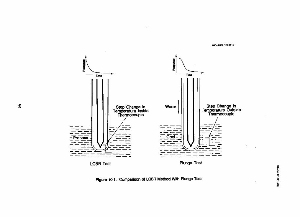
AMS-OWG THCO31B
i i _
1me
- Process
V m
Step Change in Temperature Inside
Thermocouple
Warm Step Change in Temperature Outside
Therrnocouple
- - C o o l ~ i -
LCSR Test Plunge Test
Figure 10.1. Comparison of LCSR Method With Plunge Test.
]> m 0 n - I ,= ( D

AEDC-TR-91-26
between the hot junction and the medium (fluid) surrounding the thermocouple may be
represented by a lumped parameter network such as the one shown in Figure 10.2. For this
network, the transient heat transfer equation for node i is written as~:
dT~ 1 (T~_~ - T~) - 1 ( T ~ _ T~.z) (103) m c t i t - R 1 R-'- 2
where m and c are the mass and specific heat capacity of material in the node, and R z and R 2
are the heat transfer resistances. Equation 10.3 may be rewritten as:
(10,4) d--~ ffi a i'i - I -~l i'i
where
1 ~l i , i - 1 -
m c R 1
1 (1 + 1 ) (10.5) a j,~ - m c R 1 R 2
1 t l i , i + 1 ffi mcR--..--- 2
The nodal equations may be applied to a series of nodes, starting with the node closest
to the center ( i = ] ) and ending with the node closest to the surface (i = n):
96

AEDC-TR-91-26
AMS-DWG THcO.%.~k,
Ti-1 R
1 To
I
R 2 Ti+l
Figure 10.2. Lump Parameter Representation for LCSR Analysis.
97

AEDC-TR-91-26
dr~ - - = r l + r , dt -a~l a]z
d r , = az lT x - a = T z + azsT s
dr3 ~ /_ = a3zT z - =~3r~ . a ~ r , (lO.8)
where
dr . = an. , ._ lT, ._ l -a . . , .T , . + a , w T ~
T~ = temperature of the ith node (measured relative to the initial fluid temperature). = change of fluid temperature from its initial value.
These equations may be written in matrix form:
dt
where
~ =
T,
T2 r,
A =
;I
_ a t 1
a2t
0
0
0
0
0
a m 0 0 0 0
- a= a~ 0 0 0
a~ - a ~ a~ 0 0
an,M_ | -aB,B
0
0
0
anF
(10.8)
98

AEDC-TR-91-26
Laplace transformation gives:
[sl - A] ~(s) = 7 7"v(s) + ~( . t = o ) . (~o.9)
The solution for the temperature at the central node, x I (s), is found by Cramer's rule:
T1(s ) _ B(s) (10.10) Is1-~l
where
B(s) =
'7'i(0 ) a12 0
7"2(0 ) (s +a=) -azz 0
T3(O ) -a3~ (s+a33) -a~
0
[7".(0) + a . T e ( s ) l 0 0 0 ...
0 0
-a.,,,_i (s +a., .)
(10.11)
This Laplace transform is general for one-dimensional problems and its accuracy depends
on the number of nodes used. Equation 10.9 is solved below for two different initial conditions,
one initial condition to correspond to the LCSR test and the other to correspond to the plunge
test. In the LCSR test, the temperature in the center node (hot junction of thermocouple) is not
ambient at time t = 0, while for the plunge test, the temperature at the center node is ambient
at t = 0.
99

AEOC-TR-91-26
10.3 LCSR Equation
For the LCSR test, "i(t = O) is the initial temperature distribution, and it is a vector with '.
all entdes nonzero, meaning that the first column of B(s) in matrix 10.11 has all nonzero entries.
Evaluation of the determinants, B(s) and I s / - A I, in Eq. 10.10 gives:
G ( s ) - T1 (s) _ K (s - z x ) (s - z 2 ) . . . (s - Zn_ t ) (10.12) r v ( s ) (s - / , 1 ) (s - ~'2) . - . (s - t , , , )
where each z i is a zero (a number that causes Tl(s ) to equal zero), andPi is a pole (a number
that causes Tl(s) to equal infinity) and K is a constant gain factor that can be set equal to unity
to simplify the equation. The response Tl(t ) for a step change is obtained using the residue
theorem (assuming all distant poles):
r,(t) =
( - z l ) ( - z 2 ) . . . ( - z . _ ~ )
(-Pl) C-P2)""" (-Pn) + (i l l - Zl)C°l - Z2) "'" (,.tO] - Zn-1) epV
~ - ~h) (P~ - / ' 3 ) . " (P~ - P,,)
0,s - z , ) ~°2 - = 2 ) - . . 0 ~ - z ._ l ) ep,, + . . .
(.°2 - ~ ) (/'2 - Ps ) " - ~ 2 - ~, ,)
(10.13)
This may be rewritten as
T(t) = A o + Ale plt + Aze pzt + ...
Ao, At, ,42, • . . = f (P~, ,o2, • . . z l, z2, • . . ) •
(lO.14)
Equation 10.12 is referred to as the LCSR transfer function (G ccsR) and Equation 10.14
is referred to as the equation for the LCSR transient. If the data for a LCSR test is mathematically
100

AEDC-TR-91-26
fit to Equation 10.14, the values of P l , P2, • • • can be identified and used to construct the
plunge test transient. .
10.4 Plunge Test Equation
For a step perturbation of fluid temperature, T F (s) is nonzero, but ~ (t = O) has all zero
entries because the initial temperature distribution is fist and equal to the initial fluid temperature.
In this case, the first column of B(s) contains all zeros, except for the last entry.
In this case, B(s) from matrix 10.10 may be written as:
B(s)--
0 a n 0
0 (s+a2z) -a m 0
0 -a32 (s+as3) -aa4.
0
a.F Tr (s ) 0 0 0 -a .,._~ (s +a .,.)
Using the Laplace expansion method for evaluation of the determinants, we obtain:
B(s) = a~r,~(s) (-1) "÷~
-an 0 0
(s +a22) -a23 0
-a~. (s+au) -as4
0 -a43 (s+a44)
o ° ,
* * j ,
o * °
- a ~ , . .
* . l
* * °
(10.15)
(10.16)
101

AEDC-TR-91-26
This is a lower diagonal matrix, and its determinant is the product of the diagonals:
Therefore:
B ( S ) = a , , , T , , ( s ) ( - 1 ) " * I ( a z 2 a z z a z 4 . . . ) • (10.17)
a.FrpCs)(-D "*1
T l (s ) = (s-~,,)Cs-p~)... (s-j,.) (10.18)
rl(s) and the transfer function ~ is:
T ~ ( s )
G ( s ) = K (10.19) ( s - p l ) ( s - P 2 ) "'" ( s - P 2 )
where K is a constant that can be set equal to unity to simplify the equation. By using the
residue theorem, we obtain the following expression for the fluid temperature step change
1 (Laplace transform of a unit step, i.e., T F (s) = m
$
r~(t) = 1 + 1 ep: (-p,)(-p~) ... ( -p . ) P1~1-P2) (Pt-P3) "'" O~x-P.)
] e p Z t + . . . +
. o 2 0 ~ , - p l ) ( P , - p 3 ) . . . (P,-P3)
This equation may be written as:
(10.20)
T l ( t ) = B 0 + B l e pit + B 2 e pzt + . . .
Bo , B 1 , B 2 " • " = f ( P l ' P 2 ' " " ")
(10.21)
102

AEDC-TR-91-26
The following observations can be made about the fluid temperature step change (plunge) case:
1. The exponential terms (pl, p ~ , . . . ) are the same as those of the LCSR result. This is expected since the exponents depend only on the heat transfer resistances and heat capacities, and these are the same in both ceses.
. The coefficients that multiply the exponentials are determined by the values of the poles but not of the zeros. Therefore, a knowledge of the poles alone is sufficient to determine these coefficients and the exponentials.
1 0 . 5 I . C S R T r a r m f o r m a t l o n P r o c e d u r e
The results of the dedvstions carried out above are used with the following procedure to
convert the LCSR transient to give the equivalent plunge test transient:
.
.
Perform a LCSR test and sample the data with a computer. Figure 10.3 shows a laboratory LCSR transient for a thermocouple tested in air. Normally, the LCSR trenslent starts at a high output value when the LCSR test begins and decreases as the thermocouple cools to the ambient temperature. However, it is customary to invert the LCSR transient and show it from low to high as displayed in Figure 10.3.
Fit the LCSR data to the following equation and identify thep~'s. The A i ' s do not have to be identified.
T ( t ) ffi A o + A I ~ 1' + A z ~ 2' + . . . . (10.22)
.
.
Use the pi 's identified above in Equation 10.20 to construct the temperature response that would have occurred if a fluid temperature step had been imposed.
Use the transient identified in step 3 to obtain the time constant of the thermocouple by determining the time that it takes for the transient to reach 63.2 percent of its final steady state value. Another approach, which is more often used to obtain the time constant, involves substituting the
P ~ , P 2 , • • • (or ~'1, T2, T3, • • .) in Equation 8.24 to obtain the time constant directly. This equation is repeated here:
103

AEDC-TR-91-26
AXTIO04 10
AF#13 Air@ 13 rn/s JME002A-01A
.
Q. m 4" G) IT-
_
0 1'0 2'0 3'0 4~0 T i m e (sec)
60
Figure 10.3. LCSR Transient from a Laboratory Test of a Sheathed Thermocouple.
]04

AEDC-TR-91-26
7 = 71 [1 - I n ( 1 - ' rz) - I n ( 1 - ~ ) . . . ] (10.23) T 1 T 1
10.6 Two Dimensional Heat Transfer
The approach used above can be followed to analyze the thermocouple heat transfer
based on a two dimensional model. (e) The reader may consult Reference 8 for a derivation of
the two dimensional equation. The key results of the two dimensional analysis is that, unlike the
one dimensional case, the step response results have zeros in the transfer function as well as
poles. That is, the poles identified by the LCSR test are not all that is needed to construct the
plunge test results. However, experience with typical thermocouples in typical installations has
shown that the errors due to a minor departure from one dimensional assumptions are often not
significant.
105

AEDC-TR-91-26
11. EFFECT OF PROCESS CONDITIONS ON RESPONSE TIME
This chapter presents a method that can be used to measure the response time of a
thermocouple In a convenient medium in a laboratory and use the information to estimate the
response time in another medium or in a different test condition. This method was originally
developed for selection of thermocouples to measure the temperature of liquid sodium in certain
class of nuclear power reactors. In this application, it was crucial to know in advance that the
selected thermocouples to be installed in the reactor will have a good chance of meeting the
response time requirements when the reactor begins operation. The method has also been used
by sensor manufacturers in qualification testing of prototype sensors that are designed to satisfy
specific response time requirements. The method is not a replacement for the Loop Current
Step Response test. Rather, it is a tool for obtaining a rough estimate for the response time that
can be expected from a thermocouple when it is installed in a process under known operating
conditions and installation details.
11.1 Technical Background
The response time of a thermocouple consists of an internal component and a surface
component. The intemal component depends predominantly on the thermal conductivity (k) of
materials inside the thermocouple while the surface component depends on the ~lm heat transfer
coefficient (h). The intemal component is independent of the process conditions except for the
effect of temperature on material properties inside the thermocouple. The surface component
is predominantly dependent on the proceas conditions such as flow rate, temperature, and to
a lesser extent, the process pressure. These parameters affect the film heat transfer coefficient
which increases as the process parameters such as flow rate and temperature are increased.
106

AEDC-TR-91-26
Figure 11.1 illustrates how the response time of a therrnocouple may decrease as .is increased. l
In this illustration, the effect of temperature on material properties inside the sensor is neglected.
Another factor that should be considered in the study of process effects on response time
is the ratio of intemal heat transfer resistance to the surface heat transfer resistance. This ratio
is called the Blot Modulus (NB~) which is given by:
internal heat transfer resistance hro k surface heat transfer resistance
If the Blot Modulus is large, then the response time may change very little as h is
increased, but if Blot Modulus is small, the response time will be very sensitive to changes in h
especially in poor heat transfer media where h is small. Figure 11.2 shows the response time
of two sensors in room temperature water as a function of flow rate. One of the sensors was
teated inside a thermowell and the other one was tested without a thermowell. It is apparent that
the response time versus flow rate does not improve as much for the sensor with the thermowell.
This is because the internal resistance of the sensor-thermowell combination dominates its
surface resistance, while the intemal and surface resistances of the sensor without the
thermowell are closer to one another.
11.2 Response Time Versus Heat Transfer Coefficient
As shown in Figure 11.1, the response time of a thermocouple decreases as the heat
transfer coefficient is increased. In order to dedve the correlation between the heat transfer
107

AEDC-TR-91-26
¢,.
AMS-DWG GRF022A
h
E
oO
h
Figure 11.1.
. B
o n -
Changes in Internal and Surface Components of Response Time as a Function of Heat Transfer Coefficient.
108

AEDC-TR-91-26
1.2 MEH002A-01B
0.8- p. o O
E IF. o.e-
IE
o.4- o o o
.E_ ~ 0.2-
0 0
Sensor with Thermowell
Sensor without Thermowel]
1'o 2'o ~ Flow Rate (m/s)
60
Figure 11.2. Response-Versus-Flow Behavior of a Sensor Tested With and Without Its Thermowell.
109

AEDC-TR-91-26
coefficient and response time, we recall Chapter 8 where we showed that the time constant 0")
of a thermocouple may be written as:
m c (11.1) UA
In this equation rn and c are the mass and specific heat capacity of the sensing portion, and b r
and.4 are the overall heat transfer coefficient and the affected surface area of the thermocouple.
Note that we used the overall heat transfer coefficient, U, as opposed to the film heat transfer
coefficient, h, which was used in Chapter 8. The overall heat transfer coefficient accounts for the
heat transfer resistance both inside the sensor and at the sensor surface. More specifically, we
can write:
where :
~ o | ~-~ RLn ! R==f =
U A - 1 _ 1 (11.2)
total heat transfer resistance internal heat transfer resistance surface heat transfer resistance.
For a homogeneous cylinddcel sheath, the internal and surface heat transfer resistances
may be written as follows for a single-section lumped model~:
In (11.3) R=t - 21rk/.,
_ 1 (11.4) R ~ 2"hLro
110

A E D C - T R - 9 1 - 2 6
where :
r, ffi
k =
L =
h =
outside radius of thermocouple' radius at which the junction is located thermal conductivity of sensor material effective heat transfer length film heat transfer coefficient.
Substituting Equation 11.3 and 11.4 in Equation 11.1 and 11.2 yields :
.c , ! 11" --- - - ffi f i t 2 C + - -
UA 21rkL 2fhLr,
Since m = p xr~L we can write :
(11.5)
I ' - - 2 l k I , , , ° pCro in (L/r,) +
where p is the density of the material in the sensor. Note that the second term in Equation 11.6
is reciprocal of the Blot Modulus (N~ = hrJk).
Writing Equation 11.6 in terms of two constants C1 and C=, we will obtain :
r = C 1 +C21h (I 1.7)
where •
2
C, = pCro In (rJs) (11.8) 21:
~ (11.9) 2
111

. .
AEDC-TR-91-26
Equation 11.7 can be used to estimate the response time of a thermocouple after it is
installed in a process based on response measurements made in a laboratory. The procedure
is to make laboratory response time measurements in at least two different heat transfer media
(with different values of h) and identify C 1 and Cz. Once CL and C= are identified, Equation 11.7
can be used to estimate the response Ume of the thermocouple in process media for which the
value of h can be estimated based on the type of media and its temperature, pressure, and flow
conditions. A useful application of Equation 11.17 is in estimating the response time of a
thermocouple at a given process flow rate based on response time measurements In a
laboratory flow loop. This application is described below.
11.3 Response Time Versus Flow Correlation
A correlation for response time versus fluid flow rate is derived here by determining the
relationship between the heat transfer coefficient (h) in Equation 11.7 and fluid flow rate (u).
The heat transfer coefficient is obtained using general heat transfer correlations involving
the Reynolds number, Prandtl number, and Nusselt number which have the following
relationship:
Nu =/(Re, Pr) (11.10)
In this equation, Nu = h D / K is the Nusseit number, Re : Dup/l~ is the Reynolds number, and
Pr = C# /K is the Prandtl number. These heat transfer numbers are all dimensionless and their
parameters are defined as follows :
112

AEDC-TR-91-26
h D = K -- U =
p = =
C =
film heat transfer coefficient sensor diameter thermal conductivity of process fluid average velocity of process fluid density of process fluid viscosity of process fluid specific heat capacity of process fluid
For the correlation of Equation 11.10, several options are available in the literature for flow
past a signal cylinder. One of the common correlations is that of Rohsenow & Choi °°), and the
other is from Perkins & Leppert ("). The Rohsenow & Choi correlation is '
Nu = 0.26 Re ~ Pr °'3
and the Perkins & Lappart correlation is :
Nu = 0.26 R e °'s P r lrs for
f o r 1,000 < Re < 50,000 (11.11)
40 < Re < 10 5 (11.12)
The second correlation covers a wider range of Reynolds numbers and is probably more suited
for air, while the first correlation is more suited for water. Substituting Equation 11.11 or 11.12
in Equation 11.10 will yield :
h = C~u °'~ or h = C~u °'s (11.13)
where C~ and C~ are constants and u is the fluid flow rate. Substituting the relations given by
11.13 in Equation 11.7, we will obtain the correlation between the response time and fluid flow
rate:
• r = C 1 + C 3 u "°'~ (11.14)
o r
113
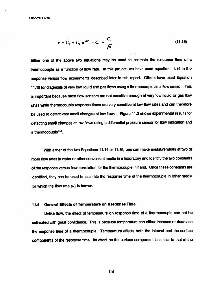
AEDC-TR-91-26
C 4 1" = C 1 + C 4 u "°'s = C 1 + ~ (11.15)
Either one of the above two equations may be used to estimate the response time of a
thermocouple as a function of flow rate. In this project, we have used equation 11.14 in the
response versus flow experiments described later in this report. Others have used Equation
11.15 for diagnosis of very low liquid and gas flows using a thermocouple as a flow sensor. This
is important because most flow sensors are not sensitive enough at very low liquid or gas flow
rates while thermocouple response times are very sensitive at low flow rates and can therefore
be used to detect very small changes at low flows. Figure 11.3 shows experimental results for
detecting small changes at low flows using a differential pressure sensor for flow indication and
a thermocouple ('~.
With either of the two Equations 11.14 or 11.15, one can make measurements at two or
more flow rates in water or other convenient media in a laboratory and identify the two constants
of the response versus flow correlation for the thermocouple in hand. Once these constants are
identified, they can be used to estimate the response time of the thermocouple in other media
for which the flow rate (u) is known.
1 1 . 4 General Effects of T e m p e r a t u r e o n R e s p o n s e T l m e
Unlike flow, the effect of temperature on response time of a thermocouple can not be
estimated with great confidence. This is because temperature can either increase or decrease
the response time of a thermocouple. Temperature affects both the internal and the surface
components of the response time. Its effect on the surface component is similar to that of the
114

AEDC-TR-91-26
AMS-DWG THC061B
e-
U-
10
0
Flow Sensor
Thermocouple Response T'rne
\ .
I I I
0 0.5 1 1.5
Flow (m/s)
v
Figure 11.3. Thermocouple Response l ime for Detection of Small Changes at Low Flows.
I15

AEDC-TR-91-26
flow. That is, as temperature is increased, the film heat transfer coefficient (h) generally
increases and causes the surface component of response time to decrease. However, the effect
of temperature on the intemal component of response time Ls more subtle. High temperatures
can cause the internal component of response time to either increase or decrease depending
on how temperature may affect the properties and the geometry of the material inside the
thermocouple. Due to differences in the thermal coefficient of expansion of materials inside the
thermocouple and the sheath, the Insulatlon material inside the thermocouple may become either
more or less compact at higher temperatures. Consequently, the thermal conductivity of the
thermocouple material and therefore the intemal response time can either Increase or decrease.
Furthermore, voids such as gaps and cracks in the thermocouple construction material can either
expand or contract at high temperatures and cause the internal response time to either increase
or decrease depending on the size, the orientation, and the location of the void. At high
temperatures, the sheath sometimes expands so much that an air gap is created at the interface
between the sheath and the insulation material inside the therrnocouple. In this case, the
response time can increase significantly with temperature.
In expedments conducted by Carroll and Shepard (2) in a Sodium loop at the Oak Ridge
National Laboratory (ORNL), more than a dozen insulated junction type K sheathed
thermocouples with Magnesium Oxide (MgO) insulation were tested for the effect of temperature
on response time. All these thermocouples were found to have a larger response time at higher
temperatures. Rgure 11.4 shows two examples of the ORNL results. The thermocouples in the
ORNL experiments were all 0.16 cm in outside diameter and were tested in flowing Sodium
116

AEOC-TR-91-26
,° t ~: o.e!
o
AMS-DWG GRF025C
0 ¢-
I -"
174 °G
/SO4 °C
I I I I I
0 0.1 02 0.3 0.4 05 Time (soc)
o
.E_ I - -
03
02.
Q
0.1 I I I I !
0 100 200 300 400 500 600 Temperature (°C)
Figure 11.4. Examples of Effect of Temperature on Response Time of Sheathed Thermocouples.
117

AEDC-TR-91-26
at approximately 0.6 cm per second. It was further determined by ORNL that the effect of
temperature on response time of different thermocoupLes is different. It was confirmed that the
effect of temperature on an identical group of thermocouples is different from one thermocouple
to another. Therefore a general response time versus temperature relationship could not be
determined for thermocouples tested by ORNL.
The above discussions demonstrate that the only way to obtain the actual response time
of a thermocouple under process operating temperature conditions is to use the Loop Current
Step Response (LCSR) method. However, when it is Impossible or impractical to perform a
LCSR test, and a rough estimate of response time suffices, the information which we have
presented in this chapter can be used in lieu of an in-situ test.
11.5 Effect of Temperature on Heat Transfer Coefficient
in this section, we will show how to account for the effect of temperature on the surface
component of response time. Neglecting the effect of temperature on the internal component
of response time, the term CI in Equation 11.14 will be unchanged. Therefore, we only need to
account for the effect of temperature on the second term of Equation 11.4.
For a given reference flow rate, it can be shown that the second term of Equation 11.4
is affected by temperature as follows (s) :
= c: , (z ' , ) h (2 ' , ) h(T2)
118

AEDC-TR-91-26
Therefore, if we know the value of constant Cj at room temperature (approximately 21°C or
70°F), we can find its value at temperature (T2) if h(70°F)/h(Tz) is known. Based on Equation
11.11 (Rohsenow & Choi correlation), we can write '
h(70°F) _ (4.3612)K(T)-CT/t (T) °-s p (T)'°~Cp (T) -°.a h(T)
(11.1 7)
From the Perkins and Leppert correlation:
h(70 °F) = (3.3603)K(-T)-~T) w p(T)-°-S°C,(T) -vs h(T)
A plot of Equations 11.17 and 11.18 for water is shown in Rgure 11.5.
(11.18)
The data in Figure 11.5 are for a pressure of approximately 140 bars ( - 2000 psi).
However, since the propertias of water are not strongly dependent on pressure, the data should
hold for pressures of up to about ± 30% of 140 bars. Note that there is a large difference
between the two curves in Figure 11.5 adsing from the use of two different heat transfer
correlations.
119

A E D C - T R - 9 1 - 2 6
N~IS.-DWG GRFO18D
12
1,1
1.0
E
~, °'
JC
0,6
os I 0
I I I I I I
1-!__ _ I __ L _I_ I _ I I I I I
+--h--~- +--l--f i I I I I I q I I I l-T
f - ~ - 1 - ~ - - I - i l I I ~T - - I-- - t - - 1- - - I - - -I-
~ l l ~ - - L 1 - - I - i - I i i i
- - I - - I I ~ _ _ ~ _ ~ - I - - ~
- I - T
I I I I I I I _ _ / _ _ I _ _ _ _ 1 _ _ / _ _ 1 _ _ _ I I i I i I
- - I - - - t - - Jr- - - I - - -I- - - t - - - i i i I i i
- - I - - - I - - 1 - - - i i I - _I-- -I _ L --I-- 4- --I-- -
I I I I I I --I-- -I - - 1 - -I-- I- - - I - - __1__ I __ L __1__ 2_ __1__ _
I I I I I I
- - I - - 4- I I
Jr- - - I - - 4- - - r - -4 - - 4- - - I - -I- - - I - - - I ~ From Perkins and Leppert Correlation I I
1- - I - 7 -F q - ~ - I- - I I- - I - - -I- - - I - - 4- - - I - - 4 ~-J~4- -~ -
i ; I ~ i i i - - - I - - 1- - - I - ~ , _ / _ l x
I I I - - - I - - + - - I-- ---I- '
I I I I - - I - T I I
i i i t 50 100
-r - 1- - I - I ~ I l~/From Rohsenow and Chol
I I I I
- - I - - M - -
I i I i 150 200
1- - I - T - i - - Correlation L I _
, i i I r - i - i ~ .4. /8 I
" T - - I - T - F- -
250 30O 350
Water Temperature (degrees C)
Figure 11.5. Correlations for Determining the Effect of Temperature on Thermocouple Response Time.
120

AEDC-TR-91-26
12. LCSR VALIDATION
A major portion of the research conducted in this project was concentrated on
experimental validation of the Loop Current Step Response (LCSR) method for in-situ response
time testing of thermocouples of the types and sizes of interest to the Air Force. The key results
of the validation work are summarized in this chapter and the details are presented in Volume II
under a separate cover. A listing of the representative thermocouples that were included in the
validation work and their pertinent characteristics are given at the end of this chapter.
The validation work described here was essential to establish the LCSR testability of
thermocoupias and determine the accuracy of the response time results obtained by the LCSR
method. More specifically, the following questions had to be addressed for types J, K, E, and
T thermocouples with wire or sheath outside diameters ranging from approximately 0.1 to 6
millimeters:
.
.
.
.
.
The optimum heating times and the current levels needed to generate suitable LCSR signals.
The cl,~, aractedstics (e.g., gain and frequency response) of amplifiers and filters to be used in LCSR testing.
The optimum sampling rates and the total sampling times that should be used in digitizing the LCSR signals for computer analysis.
The best mathematical titting algorithms and computer fdting methods to be programmed into a microprocessor for automatic analysis of LCSR data.
The effect of long extension wires and thermocouple connectors on LCSR signals.
121

AEDC-TR-91-26
.
.
The accuracy of the response time results obtained from LCSR testing of thermocouples in liquid and gaseous process media.
The minimum current levels that can be used to perform a LCSR test on a thermocouple.
The last question was addressed in light of a specific concern expressed by the Air Force
for testing of those thermocouples that'can not be given high electrical currents for the fear that
they could cause an explosion and for other process installation concerns. To accommodate
these concerns, the test equipment that has been developed in this project is equipment with
a programmable power supply that can be programmed to automatically limit the amount of
electrical currents that are used in the LCSR tests. This is discussed in more detail in
Volume III.
Based on the results of the validation research conducted in this project, it has been
concluded that the thermocouples of Interest to the Air Force are in-sltu testable by the LCSR
method and the average accuracy of the test results is about 20 percent. This exceeds the Air
Force requirement for the accuracy of the response time results. The Air Force has specified
that in-altu response time results that are within a factor of two of the true response times of
installed thermocouples are acceptable. It has been determined that when long extension wires
and multiple connectors are not involved, accuracies of as good as 10 percent can be expected
in LCSR results when optimum test currents, heating times, sampling rates, and sampling times
are used and the data is properly analyzed.
The equipment, procedures and training instructions that have been developed in this
project are intended to provide all that is needed to conduct an accurate LCSR teat and obtain
correct response time results for common thermocouple types and sizes as installed in liquid and
122

AEDC-TR-91-26
gaseous process media. The project did not specifically address the response time testing of
thermocouples that are embedded in solids or attached to solid surfaces. However, much of the
research and equipment development work completed in this project is useful in developing a
capability for response time testing of thermocouples used in media other than liquids and
gases.
12.1 Validation Results in Laboratory Conditions
The validation of the LCSR method involves a plunge test followed by a LCSR test
performed under the same test conditions on each thermocouple. The LCSR data is analyzed
and the response time results for the thermocouple is compared with that of the corresponding
plunge test to establish the validity and the accuracy of the LCSR method. For resistance
temperature detectors (RTDs), the sensor is said to be testable by the LCSR method if the
difference between its plunge test and LCSR test results is generally less than 10 percent (13).
For thermocouplas, however, a difference of 20 to 30 percent is usually used as the threshold
for expressing LCSR testability depending on the therrnocouple, the test conditions, the length
of extension wires, the number of connectors in the circuit, and the maximum current levels that
can be used to perform the LCSR test.
Table 12.1 presents typical validation results for representative thermocouplas tested in
the laboratory in room temperature water flowing at I mater per second (m/s). The reasonable
agreement between the plunge and the LCSR test results shown in Table 12.1 indicates that
these thermocouples are in-situ testable by the LCSR method. The same type results are listed
in Table 12.2 from testing of thermocouplas in room temperature air flowing at 14 m/s. Again,
the agreement between the results of the two tests are reasonable in most cases, Indicating that
the LCSR method is valid for these thermocouples as installed in flowing air.
123

AEDC-TR-91-26
TABLE 12.1
LCSR Validation Results in Water
Tag Number
Outside Resoonse Time (sec~ Diameter (mm~ ~ LCSR.
I"YPE E
44 6 1.9 1.6 27 5 1.9 1.8 29 3 1.4 1.3 43 2 0.3 0.4
TYPE J
46 6 1.8 1.5 36 5 1.4 1.1 38 3 1.8 1.4 40 2 0.4 0.4
wPE_K
4 6 2,7 2.7 7 5 2.7 2.4 9 3 0.7 0.6
13 2 0.3 0.2
Above results are from plunge and LCSR tests in room temperature water flowing at 1 meter~second.
124

AEDC-TR-91-26
TABLE 12.2
LCSR Validation Results in Air
TaQ Number
Outside Resoonse Time (sec} Diameter (mm~ ~ LCSR
TYPEE
51 Exposed Junction 1.1 0.8 43 2 3.9 4.5 29 3 10.6 12.1 27 5 17.1 22.3 44 6 23.9 32.6
TYPE J
52 Exposed Junction 1.3 1.2 40 2 3.2 3.8 38 3 9.9 12.1 36 5 17.5 21.3 46 6 24.9 35.9
TYPE K
22 Exposed Junction 0.5 0.3 13 2 3.7 3.9
9 3 10.0 11.3 7 5 17.1 23.0 4 6 25.2 29.7
Above results are from plunge and LCSR tests in room temperature air flowing at 14 meters~second.
125

AEDC-TR-91-26
Note that the thermocouple dimensions given in the tables mentioned above and in the
rest of this report are approximate values that were converted from the English units and
presented here in round numbers.
The results In Table 12.1 and 12.2 are shown graphically in Figure 12.1. This is followed
by Figure 12.2 which shows the step response of a thermocouple from a laboratory plunge test.
The signal on the top of Figure 12.2 indicates the time when the thermocouple was exposed to
a sudden change in temperature, and the signal on the bottom shows the transient response of
the thermocouple to the step change in temperature. The combination of the two signals as
shown in Figure 12.2 is referred to as plunge test data or plunge test transient. The response
time of the thermocouple is obtained directly from this data by simply measuring the time from
when the step change in temperature is imposed, to the time when the thermocouple reaches
63.2 percent of its final steady state value.
Typical LCSR transients for testing of thermocouples in water and air are shown in
Figure 12.3. These are inverted and normalized LCSR cooling transients. All LCSR transients
shown hereafter in this report are inverted and in most cases are normalized for ease of
comparison. The details of how LCSR tests are conducted and further laboratory validation
results for different thermocouple sizes and test conditions are presented comprehensively in
Volume II.
The laboratory plunge tests conducted in this project were based mostly on the methods
prescribed by the American Society for Testing and Matedals (ASTM). The ASTM methods for
response time testing of industrial RTDs and thermocouples me outlined in two standards:
126

AEDC-TR-91-26
w,,,*~ @ 1 rn/. Initial Validation DWMO12A-01B
I I 11 ~ _
1 44 27 29 43 46 36 38 40 4 7 9 13
Tag Number
Plunge Result [ - - '7 LCSR Result
J r @ 14 m/s I¢li~al VaJidatJon DVSOO1A-O1A
35-
.~. 3O
"0 C 0 0 25' G}
C 0 ¢J 15- (9 E i= 1o-
46 36 38 40 4 7 g 13 44 27 29 43 51 52 22 18
Tag Number
Figure 12.1. LCSR Validation Results in Water and Air.
127

AEDC-TR-91-26
3D: 2 5 M < 1 5 : 0 4 : 5 4 , - 0 5 .3"UN 9 0 = S P D : 5 M M / S ( 2 0 0 . 0 M S / M M )
" !"i : :. [i.iiiii...i i.i.i.i i i i ii i I i . i i i i i i i:ii i iii':i.i i i " i , i i . i i.! !::
• i.,ji~.il i i ii iii~ . ~ i . i . ~
i !
Figure 12.2. A Typical Plunge Test Transient.
128

A E D C - T R - 9 1 - 2 6
AF 11
,o] DVS014A-01A
Water 1 m/s
O (n t -
g q~
n "
Air 14 m/s
1-
1'0 1'. Time (seconds)
30
Figure 12.3. Typical LCSR Transients in Water and Air.
129

AEDC-TR-g 1-26
1. ASTM Standard E839-89 entitled, "Standard Test Methods for Sheathed Thermocouples and Sheathed Thermocouple Material'.
2. ASTM Standard E644-86 entitled "Standard Methods for Testing Industrial Resistance Thermometers".
These Standards are published in the annual book of ASTM standards (14'1s). There is no standard
for LCSR testing of thermocouples. The only standard that relates to the LCSR method is that
of the Instrument Society of America (ISA) for RTDs (1~. Referred to as ISA Standard 67.06, this
standard outlines the acceptable methods for response time testing of safaty-related sensors in
nuclear power plants. It'includes the LCSR method for in-situ response time testing of RTDs as
installed in nuclear power plants.
12.2 Validation Results in Wind Tunnels
Since many aerospace applications involve temperature measurements in high air
veloc'rties, some LCSR validation tests were performed at flow rates beyond what could be
generated in the laboratory air loop that was constructed for this project. Thus, the high flow
tests were performed in the subsonic and supersonic wind tunnels at the Mechanical and
Aerospace Engineering Department at the University of Tennessee in Knoxville (UT). In the
subsonic tunnel, a system was sat up to permit plunge testing, but in the supersonic tunnel,
plunge tests could not be performed. Therefore, the thermocouples that were selected for the
supersonic tests were plunge tested in the AMS laboratory and their response time results were
extrapolated to the supersonic flow conditions using the guidelines given in Chapter 11.
Table 12.3 presents the results of the LCSR validation tests performed in the subsonic
wind tunnel for three air flow rates. The results for 60 and 100 miles per hour velocities are
presented graphically in Figure 12.4. The reasonable agreements between the plunge and the
LCSR results testify to the validity of the LCSR method for testing of these thermocouples.
130

• : , A E D C - T R - 9 1 - 2 6
TABLE 12.3
LCSR Validation Results in Subsonic Wind Tunnel
Tag Number
ResDonse Time ~sec~ LCS_ BR
27 m/oec - 60 mlles/hr
14 15 16 22 29 40
1.4 0.7 1.7 0.4 8.0 2.5
1.2 0.8 1.5 0.5 9.1 4.4
45 m/sec - 100 mlles/hr
14 15 16 22 40
1.2 0.4 1.1 0.3 2.2
2.0 0.3 1.0 0.4 3.0
55 m/sec ,, 123 m l l u / h r
29 6,0 6.3
131

AEDC-TR-91-26
UT~?' m/e DWIk~0A-01A
I i
i '- =_ =. .,
14 15 18 22 29 40
Tag Number
Plunge Trot ~ LCSR Test
UT4S m/e 4
OWM020A-0~.A
1o | o E i= =,- O Q.
n-
14 1~ lU ~ 40
Tag Number
Rgure 12.4. Representative Results of LCSR Validation Tests in Subsonic Wind Tunnel.
132

AEDC-TR-91-26
The results from the tests in the supersonic tunnel are given in Table 12.4. These results
are from the LCSR tests in the supersonic tunnel at Mach 2, The reasonable agreement between
the plunge and LCSR results shown in Table 12.4 indicates that the LCSR method is valid for
these thermocouples at supersonic flow conditions. Typical LCSR transients for two of the
thermocouples tested in the supersonic wind tunnel are given in Figure 12,5,
12.3 LCSR Software Quallflcatlon
In Chapter 10, we covered the theory of the LCSR method and presented the analysis
procedure for obtaining the response time of a thermocouple using the LCSR data. The analysis
is needed because the LCSR data is obtained by internal heating of a thermocouple while the
response time of Interest should result from a step change in temperature outside the
thermocouple. Therefore, the LCSR data must be converted by a mathematical fitting procedure
implemented on a computer to transform the LCSR data to an equivalent plunge test transient
and yield the response time of the thermocouple tested. The details of the mathematical
equations and procedures for the transformation of LCSR data were covered in Chapter 10.
Three independent algorithms were developed in this project and tested for computer
analysis of LCSR data for various thermocouples. These developments took advantage of our
earlier work on LCSR analysis of Resistance Temperature Detectors (RTDs) in nuclear power
plant applications. An analysis technique and a software package called "Time Sedes Fitting or
TSFI'r" that had been developed for RTDs was found to be equally useful for thermocouples.
The results of LCSR analysis with the TSFIT package are shown in Table 12.5 and compared
with the results of two other techniques implemented in two computer codes called LST-SQ and
133

AEDC-TR-91-26
TABLE 12.4
LCSR Validation Results in Supersonic Wind Tunnel (Mach 2)
Tag Response Time fsec} @ 14 mlsec Number Plunae
18 0.14
20 0.16
22 0.49
23 0.50
Resoonse Time (sec~ ~ Mach 2 Plunae* LCSR
0.05 0.05
0.05 0.04
0.06 0.06
0.06 0.08
* E.~mpolated from laboratory measurements.
134

AEDC-TR-91-26
AF&~015 AF#20 @ MACH 2 JMEOOIA-O3A 10'
5,
2-
0 0 o.b2 o.b4 o.b5 o.bs 0.1 Time (sec)
AFeS052 AF#23 @ MACH 2 JMEOO1A-O4A 10"
,
6.
! =54
n -
2-
0 0.05 0:1 0.:15 0:2 0.25 Time (sec)
Figure 12.5. Typical LCSR Transients from Tests in Supersonic Wind Tunnel.
135

AEDC-TR-91-26
TABLE 12.5
Results of LCSR Software Qualification
Tag Number
Response Time bv Plunoe (secl
Response Time ~sec) bv LCSR Test TSFIT LST-SQ XTCA9
4 7 9 13 27 29 36 38 38 40 43 44 46
2.7 2.7 0.7 0.3 1.9 1.4 1.4 1.9 1.8 0.4 0.3 1.9 1.8
Water ~ 1 m/s
2.6 2.4 0,6 0.2 2.0 1.2 1.2 1.7 1.4 0.5 0.4 1.7 1.5
2.4 2.2 0.5 0.2 1.7 1.2 1.0 2.1 1.8 0.3 0.3 2.1 1.5
2.1 3.2 0.5 0.2 1.6 1.8 0.7 2.3 1.6 0.3 0.3 0.16 1.2
7 7
13 27 36 36 36
17.1 17.1 0.3 17.1 17.5 17.5 17.5
Air @ 14 m/s
27.0 19.7 0.3
18.4 22.6 22.8 18.2
26.0 17.2 0.3 16.5 20.2 20.5 30.0
26.1 26.6 0.2
34.2 62.7 39,4 20.8
136

AEDC-TR-91-26
XTCA9. The results are given for both plunge tests and LCSR tests in room temperature water
flowing at I m/s and in room temperature air flowing at 14 m/s. The results for the tests in water
are shown graphically in Figure 12.6. Based on these and other similar results produced dudng
the project, it was determined that the TSFIT is the most suitable approach and it was therefore
selected for use in the microprocassor-based LCSR test analyzer that has been developed in this
project. The details of development of the LCSR analyzer are given in Volume III.
12,4 LCSR Noise Reduction
The LCSR transient for a thermocouple may contain both high frequency and low
frequency noise. For the purpose of this discussion, we define high frequency noise as those
electrical and other interferences with frequencies of 10 Hz or higher, and low frequency noise
as the low amplitude fluctuations of less than 10 Hz which often result from temperature
fluctuations in the process.
The high frequency noise is removed with a Low-Pass (LP) electronic filter. The LP filter
must be set at a frequency that is low enough to adequately remove the extraneous noise, and
at the same time is high enough to ensure that it will not eliminate any useful portion of the
thermocouple signal. The following equation provides a guide for where the LP filter should be
set at:
z z (12.1) r = - - o r F = - - 21rF 2~r~
137

AEDC-TR-91-26
water @ 1 m/s LCSR Software Qualif ication DVS006A-02A
A
09 v
¢- 0~ ~o t- O
o
E ° i
I--
4 7 9 13 27 29 86 ;]8 40 43 44
T a g N u m b e r
I Plunge TSFIT [-"-'J LSToSQR ~ XTCA9
46
Figure 12.6. LCSR Software Qualif ication Results.
138

AEDC-TR-91-26
where 1, is the expected response time of the thermocouple (in seconds) and F is a its
corresponding frequency response or comer frequency in Hz. The LP filter should be set st
about 10 to 20 times the frequency response (F) depending on the roll off rate or sharpness of
the LP filter. Figure 12.7 shows two LCSR transients with and without filtering. Note how the
high frequency noise that is apparent on the top transient in Figure 12.7 is not present in the
filtered transient st the bottom.
12.5 Averaging of LCSR Data
To reduce the effect of low frequency noise, the LCSR test is repeated 10 to 30 times and
the raw data is simply averaged to provide a smooth transient to facilitate the analysis and yield
accurate results. Figure 12.8 shows three LCSR transients as follows: a single transient, an
average of 10 transients, and an average of 20 transients. Note that averaging can effectively
eliminate the low frequency noise on the LCSR data, and that the average of 10 single LCSR
transients is usually adequate, as apparent in the case shown in Figure 12.8. Most of the LCSR
transients that are shown in this report are the average of 10 data sets.
A key point in implementation of an averaging scheme is the identification of the exact
beginning of the LCSR transient. It is important for the LCSR transients that are averaged to start
at the same time into the data or the averaged transient would be distorted and will give
incorrect results.
139

AEDC-TR-g 1-26
UNFO001-10 1
AF#43 AIr@14m/s 0.35A OVSO12A.O2A
0.8"
o ~>
o. 0.6- !5 0 _e O. :3
0.4-
o
0.2-
0 0 1'0
_ . . - - -
Time (sec)
. = = I
30
RL0001-10 1.
AF#43 Air@ 14 rn/= 0.35A DVSO12A-O1A
0 . 8 "
0.6. o
~0.4'
0.2'
G 0 1'0 ;~0 30
Time (see)
Figure 12.7. LCSR Transients W'~h and Without Filtering.
140

AEDC-TR-91-26
10-
9-
7-
6.
"~L 5"
3"
2"
1'
AF#13 W=t..r I m.~ Dv~+~.me
Time (m=)
~ff[R 011t.ot~ AF#13 Walw I INs m~s'zA-~ 10
/
0 o i
Tune (see)
VF3i0111-01~10 AF#13 W=dlm' I m/s mS~tA.e~ 10
9,
7'
i s.
I' 3'
2'
Time (~ )
Figure 12.8. A Single Raw LCSR Transient (top), Average of 10 Transients (Middle), and Average of 20 Transients (Bottom).
141

AEDC-TR-91-26
12.6 LCSR Parameter Optimization
A number of parameters are involved in performing a LCSR test and analyzing the data.
These parameters must be sat at correct values to yield accurate LCSR results. The challenge
is that these parameters are often interactive meaning that a change in one affects one or more
of the others.
The LCSR data for a thermocouple that is expected to have a response time in the
neighborhood of 0,10 seconds is sampled much faster and for a much shorter length of time
than the data for a thermocouple that is expected to have a 10 second response time. The
optimum values for these two parameters depend on the expected response time of the
thermocouple under the condition that it is tested. Several other parameters are involved in a
LCSR test. A description of these parameters and how to properly select them is presented
below.
Heatina Current. The LCSR test of a thermocouple requires a heaUng current of about 0.3 to 3.0 amperes depending on the size (diameter) of the thermocouple, the length of the extension wires, and the process conditions in which the thermocouple is used. The rule-of-thumb is to start with a small current and increase it as necessary to obtain a reasonable LCSR transient. Figure 12.9 shows three raw transients that are labeled as reasonable, borderline, and not acceptable for accurate response time determination.
A number of remedies are available for improving the quality of a LCSR transient. The first and usually the most effective remedy is to use a higher heating current if possible. Figure 12.10 shows how the quality of a LCSR is improved by increasing the heating current while keeping the other test parameters constant.
There are two problems with using high heating currents. One is safety, and the other is the possibility of creating large temperature gradients in the thermocouple extension wires and connectors. A large gradient together with any inhomogeneity in the thermocouple circuit can result in EMF transients that are not related to the thermocouple junction, but are superimposed on the LCSR signal.
142

AEDC-TR-91-26
1" U R ~ AIEN~IA
0.B'
0.6'
0.4'
o Jr dO 4"o ~o ~o !
11me (mmoncls)
Border Une ,mBoB~m 8UBOOtll
t 0.6
0.4
0
lo 20 ~o /1me (seconds)
40
0.B"
CI• 0.4"
0.2'
0
NFI14M2 1~loJloltmbkl
J 1"0 dO dO ~0 5~
Time (seoonds) 60
Figure 12.9. LCSR Transients of Varying Quality.
143

AEDC-TR-91-26
0,8-
i 0.6-
0.4-
i • 0.2-
0
o.tsk~m AF#43 WWetr 14 I1~ o w m ~
6 1"0 1"5 2"0 2"5 Time {See)
30
~aokmm,~ AF#43 Wslm 14 m/-, ovm:*,.m* 1.
E" ~0" £
~ 0.6.
tt
J°.' t 0.2
0 • • 0 5 10 15 20 25 Time (sec)
30
uo*m~m AF#43 Water 14 m/s o m ~ 1.
0.8.
0.8, O
j 0.4
0.2
0 o 5 lO I"5 L~ 25
Time {eat) 30
Figure 12.10. Quality of LCSR Transient Versus Applied Current.
144

AEDC-TR-91-26
Another remedy is to use a small heating current but a large amplifier gain to improve the dynamic range of the LCSR transient. The problem with a large gain is the possibility of introducing high frequency noise on the LCSR signal. This problem can be resolved using a low-pass filter as was explained in Section 12.4. above. There is always a trade off between the heating current, the amplifier gain, and the low pass filter setting. Another parameter that is highly linked with the heating current is the heating time as described below.
Heatinu Time. The amount of LCSR heating in a thermocouple depends not only on the applied current, but also on the heating time. Generally, the heating time should be long enough to allow the thermocouple junction to reach steady state. A good rule is to apply the heating current for about 5 to 10 times the expected response time of the thermocouple under the conditions of the test. Longer heating times do not usually have an adverse effect on the LCSR data except when there is an inhomogeneity in the thermocouple circuit. In this case, a long heating time can produce large temperature gradients that can adversely affect the LCSR transient when the current is cut off. More specifically, the effect can manifest itself in terms of an upward or downward drift on the steady state portion of the LCSR transient.
In the experiments that were conducted in this project, heating times of 5 to 15 seconds were used. A serias of experimants were performed specifically to address the effect of heating currents and heating times on the LCSR results. Key results of these experiments are summarized graphically in Figure 12.11 for 5 and 15 second heating times. These results are from LCSR testing of thermocouples in room temperature water flowing at 0.6 m/s. They are shown for three current levels: low current, medium current, and high current. The current levels were 0.25, 0.5, and 1.0 amperes for thermocouples with 23, 24, and 30 gage wires, and 0.75, 1.0, and 1.5 amperes for thermocouples with 18 and 20 gage wires. The data in Figure 12.11 are given in terms of percent difference between the LCSR results and the corresponding plunge test results.
Amnlifier Gain. In LCSR testing of thermocouples, it is usually desirable to have signal amplitudes of near 10 volts even though signal amplitudes as low as 1 volt are often acceptable. In the laboratory LCSR tests that were conducted in this project, depending on the thermocouple being tested and the test conditions, the required amplifier gains were 20,000 to 500,000 for a 10 volt signal. The lower gains were used for the small diameter thermocouples, and the higher gains were used for large diameter thermocouples. For the tests in air, smaller gains were usually adequate, but for the tests in water, larger gains were generally required. This is because in the air tests, due to poor heat transfer, thermocoupias heat up more for the same amount of current than they do in water.
Low-Pass Filter Settino. The LCSR test equipment for thermocouples often require a low-pass (LP) filter. The LP filter is required to remove the high
145

AEDC-TR-91-26
C U ~
i -r D ~ ~ m
~-i~ "~
-li! II- o 29 34 40 43
Teg Number
e
a-
]
I.o n N
3G
z
I o
W
1 N
-1E . . . . . . . . . 4 7 ~ ' 25 N N 40 43 44 M
Tag Number
I~amp¢ JJG~OI~t0C
i - H t ~ - ~
l 4 ' 7 " 27 ' 30 ' 44 " M
Tag Number
Figure 12.11. Differences Between the LCSR and Plunge Test Results for Three Levels of LCSR Heating Currents.
146

AEDC-TR-91-26
frequency noise which is often present on the LCSR signals due to high amplifier gains that are usually necessary for the LCSR tests. Furthermore, thermocouples are inherently susceptible to electrical noise pick up which contaminate the LCSR data and interfere with a successful analysis. The high frequency noise should be removed using a low-pass filter that is properly set for the application in hand. The filter setting depends on the amplitude and frequency of the interfering noise. In the laboratory tests that were conducted in this project, LP filter setting of 10 to 30 Hz were often used depending on the size of the therrnocouple, the heating current, and the test conditions.
,Semolina Rate. A 12-bit analog-to-digital converter (also referred to as A to D, ADc, or A/D) was used in all the LCSR tests that were conducted in this project and in the test equipment that was developed. The A/D was adjusted for 0 to 10 volt range for the LCSR signals. Depending on the expected response time of the thermocouple being tested, sampling intervals of 0.005 to 0.1 seconds (10 to 200 Hz) were used. The smaller sampling intervals were used in testing of the faster thermocouples and the larger sampling rates were used in testing the slower thermocouples. Although it was not attempted in the project, the use of a 16-bit A/D could have helped reduce the high amplifier gains that are required for LCSR testing of thermocouples.
Total Number of Samoles. The total number of points that are sampled in a LCSR test depends on the sampling rate and the time that it takes for the LCSR transient to reach steady state. The product of the sampling rate and the total number of points sampled should exceed the time that it takes for the LCSR signal to reach steady state. This time is referred to as sampling time which ranges from a few seconds to several tens of seconds, depending on the size of the thermocouple being tested and the test conditions. The tests in air generally required longer sampling time and/or large sampling rates than the tests in liquids.
Number of LCSR Transients to Averaoe. The high frequency noise and low frequency fluctuations that usually exist on the LCSR signal must be removed or minimized to yield accurate response time results. The high frequency noise is removed by a Iow-pess filter, and the low frequency fluctuations are minimized by averaging a group of identical tests on the same thermocouple. Since the low frequency fluctuations usually originate from the process due to random temperature fluctuations, an ensemble averaging can reduce the fluctuations without affecting the dynamic characteristics of the data.
The number of single LCSR transients that are averaged together depends on the amount of fiuctuations on the data. In the experiments that were conducted in this project, 10 LCSR transients were found to be adequate in most cases even though 20 transients were sometimes used. In field tests, it may be necessary to repeat the LCSR test as many as 30 times and average the single transients to obtain a smooth data set for optimum analysis. The test equipment that was developed in this project can readily be programmed to repeat the tests automatically for the number repeats specified by the user.
'- 147

AEDC-TR-91-26
12.7 LCSR Difficulties
Both AMS and the Oak Ridge National Laboratory (ORNL) (2'e), who have worked
extensively on LCSR testing of thermocouples, have had a common difficulty arising for inherent
inhomogeneitias that are sometimes present in thermocouple circuits. The inhomogeneities can
exist in the extension wires, connectors, or even inside the thermocouple itself.
Shepard and Carroll (e) noted that each LCSR transient for a thermocouple is the resultant
of three separate transients illustrated in Rgure 12.12. In this figure, trace 1 illustrates the
cooling transient of the therTnocouple junction which we wish to measure. Trace 2 illustrates a
transient due to an inhomogeneity in the circuit, and trace 3 is from the magnetic effect that may
be present at the LCSR output of a type K thermocouple. In Figure 12.12, traces 2 and 3 are
exaggerated to make the point more clear. In actuality, these traces are not nearly as large in
amplitude as they are shown.
In testing of a type K thermocouple in stagnant and stirred water, ORNL obtained two
widely different LCSR transients as illustrated in Figure 12.13. This probably occurred due to an
inhomoganeity in the thermocouple circuit producing a transient that competes with the LCSR
transient. When the water is stagnant, the LCSR transient dominates because it is apparently
much slower and larger in amplitude than the interfering transient. When the water is stirred, the
interfedng transient dominates because the junction transient is faster and decays much quicker
than that of the Interfering transient. An investigation into these types of effects revealed, in one
instance, that the inserts in the connectors of a thermocouple ware manufactured with a wrong
alloy.
Similar results have been observed by AMS as illustrated in Rgure 12.14 and 12.15. In
each of these two figures, the resultant transient is illustrated on the top and its potential
148

AEDC-TR-91-26
LL
UJ
AMS-DWG GRFO24A
Ambient Temperature
Time (sec)
Figure 12.12. Illustration of Potential Components of a LCSR Test Transient.
149

AEDC-TR-91-26
AMS-DWG GRFO23A
LL
LU
nant Water
Water
Water Temperature
Time (sec)
Figure 12.13. Illustration of Unusual LCSR Transients for a Thermocouple in Stagnant and Stirred Water.
150
AEDC-TR-91-26
/~IS - P.Y,'G GRF021C
.! Junction Response
o ¢- ¢- o o _¢
O o o
e - I---
/ \
\ / /
/ / Connector
Effect
Time
¢z
O
n-
O ..J
/ i i
I
Resultant LCSR Transient
Time
Rgure 12.14. Illustration of Possible LCSR Transients for Thermocouple Circuits With Gross Inhomogeneities,
151

AEDC-TR-91-26
, !
!AMS-DWG GRF020B
t,o
8
8 O
ction Response
Connector Effect
Time
(3.
O ¢0 Q)
}--
n~ of) C~ ._1 Resultant LCSR Transient
Time
Figure 12.15. Illustration of Possible LCSR Transients for Thermocouple Circuits W'dh Gross Inhomogeneities.
152

AEDC-TR-91-26
components are shown on the bottom. Two actual LCSR transients showing the two most
commonly observed inhomogeneity effects are presented in Figure 12.16. These data are from
LCSR testing of thermocouples in laboratory conditions.
12.8 LCSR Test for Detection of Thermocouple Inhomogeneitles
There is a positive aspect to the LCSR difficulties discussed above. That is, the ability
of the LCSR test as a method for diagnosis of gross inhomogeneiUas in thermocouple circuits.
In an experiment conducted in the early 1980's at the Argonne National Laboratory in Chicago,
the author and others were involved in LCSR testing of a group of thermocouples that were
being prepared for installation into a nuclear radiation experiment. The unusual LCSR transients
that were initially observed in these thermocouples provided a clue that there was a problem in
the thermocouple circuits. Further investigations revealed that the thermocouplas were
inadvertently reversed in their connectors during Installation. The problem was corrected and
the thermocouples were LCSR tested successfully. Figure 12.17 shows two LCSR transients
for a thermocouple that was first installed in its connector correctly and then reversed to show
how the LCSR can reveal the problem.
12.9 Effect of Extension Wire and Connectors
Long extension wires and connectors sometimes present problems in LCSR testing of
installed thermocouplas. The problem is often exasperated by inhomogeneitlas in the extension
wires or in the connectors where the extension wires are attached to the thermocouple wires.
The. effect of connectors on LCSR signals were covered in Phase [ as documented in our
Phase [ report (~'/).
153

A E D C - T R - 9 1 - 2 6
m
I''I
I
Figure 12.16. Actual LCSR Transients for Thermocouples With Circuit Inhomogeneities.
154

AEDC-TR-91-26
AF'8,S~. Wmr, E Normal • REFOO17A,.OIA
l CO I N " v
8, 4.
.
6 10 20 30 40 50 60 70 Time (see)
AF21,Stag. Watm, E Reversed REFOO17A-O~
t ._ca (o fT. o'J o,
1 0 20 40 60 80 100 120 140
Time (seo)
Figure 12.17. LCSR Transients for a Normal and a Reversed Installation of a Thermocouple into its Connector.
155

AEDC-TR-91-26
The effect of extension wires on the results of the LCSR tests and other difficulties that
may be encountered in LCSR testing of thermocouplas are discussed in detail in Volume [I.
Also shown in Volume 1[ are experimental results with different types and lengths of
thermocouple extension wires. An example of such results is shown in Rgure 12.18 for a group
of thermocouples teated in water. These data represent the percent differences between the
results of LCSR and plunge tests performed under the same conditions with three different
lengths of thermocouple extension wires. Note that there is not a good correlation between the
LCSR error (present difference between the results of plunge and LCSR tests) and the length of
the extension wires. That is, the accuracy of the LCSR test results is not always adversely
affected by increasing the length of the extension wires.
12.10 Harmful Effects of LCSR Test
LCSR method is generally a safe test if it is performed properly and with adequate care.
However, there is some potential for harmful effects to the thermocouple circuits and electrical
hazard for the test personnel. These should be taken into account and guarded against in the
LCSR process. In the three years that this project was actively pursued at AMS, there was no
incident during the LCSR experiments even though many engineers and technicians worked on
this project.
Volume [I presents the results of experiments performed to assess the potential for
damage to the extension wires or the insulation of the wires from LCSR testing. The data from
these experiments have revealed that the LCSR test does not normally jeopardize the health and
integrity of the wires as long as the LCSR current levels and heating times are maintained at a
reasonable level.
156

AEDC-TR-91-26
60.0
Water @ 0.6 m/s DWM014A-011
50.0'
40.0
~ 0.0
~" 2O.O
~ 10.0
~ 0.0
-10.0 u _
-20.0
-30.0
N
Ip I I I I I I
07 04 27 44 36 Tag Number
I S m IF"~9m I--'-1,15m
38
Figure 12.18. Error of LCSR Results Due to Extension Wires.
157

AEDC-TR-91-26
It is important for the users of the LCSR method to be aware of the heating that is
produced in the thermocouple circuits dudng the LCSR test. It is also important to point out that
the LCSR test sometimes involves potentially harmful electrical currents that must not come into
contact with the test personnel when the thermocouple is under test. The equipment and
procedures that were developed in this project have been designed with safety in mind. The
safely features of the equipment are descdbed In Volume III. Two examples of these features
are:
.
.
An option for the user to program the AC power supply in the equipment for a limited current output.
A safety cover on the cold junction copper blocks in the equipment that turns the current off when the cover is removed.
12.11 Description of Project Thermocouples
Table 12.6 presents a listing of most of the thermocouples that were included in the tests
described in this chapter. A tag number was assigned to each thermocouple to facilitate the
presentation of the research data we produced in the project. Most of these thermocouplas and
the extension wires that were used In the project were purchased from Omega Engineering
Incorporated, located in Stamford, Connecticut, USA. There was no particular reason for the
types, sizes, physical cordigurat.ions, and the manufacturer of the thermocouples that were
selected for the project other than the fact that these thermocouplas comply with the types and
sizes that were specified by the Air Force for this project.
12.12 Effect of Heating Time on LCSR Results
We mentioned eadier that the LCSR heating time does not play a major role in the quality
and accuracy of the LCSR test results. Of course, the heating time must be long enough to
158

AEDC-TR-91-26
TABLE 12.6
Usting of Thermocouples Used in the Project
Number AF#I
AF#2
AF#3 AF#4
AF#5
AF#6 AF#7 AF#8 AF#9 AF#10
AF#11 AF#12
AF#13 AF#14
AF#15
AF#16 AF#17 AF#18 AF#19 AF#20
AF#21 AF#22
AF#23 AF#24 AF#25
AF#23 AF#27 AF#23
AF#23 AF#30
Gaco ~ LoooR K Quick-Disconnect 18 1/4 0.61
K Quick-Disconnect 18 1/4 0.63 K Quick GND-JNC 18 1/4 0,45 K Quick-Disconnect 18 1/4 0.65
K Quick-Disconnect 18 1/4 w
IR 200K 40M
n/a 25M
>IOOG
K Quick-Disconnect 20 3/16 0.69 200 K K Quick-Disconnect 20 3/16 0.66 500 M K Trans 36" 20 3/16 2.27 1.5 M K Qulck-Disconnect 23 1/8 1.40 10 M K Quick-Disconnect 23 1/8 1.67 15 M
K Quick-Disconnect 23 1/8 1.58 K Trans 40" Bent 23 1/8 3.55 K Quick-Disconnect 30 1116 5.11 K Quick-Disconnect Flex 1.72
K Quick-Disconnect Flex
K Quick-Disconnect Flex 1.2 K Quick-Disconnect Flex 4.63 K Q-mini EXP-JNC 0.053 113.4
K No CON EXP-JNC 0.053 K Q-mini EXP-JNC 0,052 111.4
K Q-mini GND-JNC 0.053 284 K Q-mini EXP-JNC 0.16 11.6 K Q-mini EXP-JNC 0.16 10.9 K Q-mini GND-JNC 0.052 14 K Q-mini GND-JNC 0.052 13
1M n/a
4M n/a
n/a
n/a n/a
200 K
150 K
I1/8 200K 350K
n/a n/a
E Trans 40" 20 3/16 2.87 40 M E Qulck-Oisconnect 20 3/16 0.79 35 M E Quick-Disconnect 20 3/16 0.77 10 M E Quick-Disconnect 23 1/8 1.57 30 M E Tram 51" 20 1/8 4.35 90 M
159

AEDC-TR-91-26
TABLE 12.6 fcontinued)
Number
AF#31 E Quick-Disconnect AF#32 T Trans 40"
AF#33 T Quick GND-JNC AF#34 T Quick-Disconnect AF#35 T Quick-Disconnect
AF#36 J Traps 29" AF#37 J Quick-Disconnect AF#38 J Quick-Disconnect AF#39 J Trans 51" AF#40 J Quick-Disconnect
AF#41 E Dual PH assmb. AF#42 T Dual PH assmb.
AF#43 E Quick-Disconnect
AF#44 E Quick-Disconnect AF#46 E Quick-Disconnect
AF#46 J Quick-Disconnect AF#47 J Quick-Disconnect AF#48 J Quick-Disconnect AF#46 K Quick-Disconnect AF#50 K Quick-Disconnect
AF#51 E Quick EXP-JNC AF#52 J Quick F.XP-JNC
eaco ~ LoooR IR
30 1/16 6.15 300 M
20 3/16 1.62 13 M 20 3/16 0.47 n/a 20 3/16 0.41 5 M 30 1/16 3.07 10 G
20 3/16 1.47 10 G 20 3/16 1.03 6.5 M 24 1/8 1.28 6 M 20 1/8 2.76 10 M 30 1116 3.29 1.2 M
1/4 0.5 10 G 1/4 0.45 n/a
1/16 6.9 20 M 1/4 0.85 400 K
1/16 7.2 7 G
30 18 30
18 1/4 0.6 1.5 M 30 1/16 3.75 10 G 30 1/16 4.0 20 G 30 1116 5.8 20 M
30 1/16 5.8 20 G
30 1/16 6.3 4.0 M 30 1116 3.7 1.2 M
OD: Outside Diameter.
IR: Insuldon Resistance.
]60

AEDC-TR-91-28
allow one thermocouple to reach steady state above thetemperature of the surrounding
medium. During this project, we determined that a heating time of between 5 to 15 seconds is
generally adequate for the thermocouples that were involved in this project (see Table 12.6) and
under the laboratory conditions in which they were tested. Figure 12.19 shows the LCSR errors
for heating times of 5 and 15 seconds. The errors represent the percent difference between the
thermocouple time constants obtained by the plunge and LCSR tests under the same conditions.
The results in Figure 12.19 indicate the magnitude of errors are generally the same for either 5
or 15 seconds of heating meaning that any heating time in the 5 to 15 second range is adequate
for LCSR testing of these thermocouples in water.
161

AEDC-TR-91-26
Water @ 0.6 m/s Heating Current = 0.5 amp JJG006A-07C
o,
J m
D
9 29 38 40 43 Tag Number
5 Seconds ~ 15 Seconds
Figure 12.19. Optimum Heating Times for LCSR Testing of Thermocouples.
162

AEDC-TR-91-26
13. LCSR TEST INSTRUMENT
A photograph of the LCSR test instrument that was developed in this project is shown
in Figure 13.1. This instrument can be used to perform both the LCSR test and the associated
date analysis. The details of how this equipment was developed including its operations and
maintenance manual, manufacturing procedure, and parts list are given in Volume IIL The kay
points regarding the development and operation of the Instrument are presented in this chapter.
The LCSR test instrument as shown in Rgura 13.1 consists of two separate units. One
is used to perform the) LCSR test and generate the raw data, and the other Is used to analyze
the date and display the results. The first unit is named ETC-2, and the second unit is named
ESA-1.
A photograph of ETC-2 is shown in Figure 13.2. This unit is an upgraded version of
ETC-1 which was used in the Phase I project. A major difference between ETC-1 and ETC-2 is
in the LCSR signal conditioning amplifiers and filters. In ETC-2, the amplifiers and filters are built
into the unit, while in ETC-1, the signal conditioning equipment were used as separate equipment
outside the unit.
A photograph of ESA-1 is shown in Figure 13.3. Both the front and back panels of the
unit are shown. The ESA-1 was completely designed and assembled at AMS as a major part
of this Phase 1I effort for AEDC. A block diagram of ESA-1 is presented in Figure 13.4. This unit
is basically a dlsklass microcomputer with an Intel 386, 20 MHz microprocessor module. The
system was designed and developed specifically for LCSR data acquisition and date analysis
163

AEDC-TR-91-26
• I
Rgure 13.1. Complete LCSR Test Instrument.
164

AEDC-TR-91-26
Figure 13.2. LCSR Signal Generator ETC-2.
165

AEDC-TR-91-26
FRONT PANEL
BACK PANEL
Figure 13.3. LCSR Test Analyzer ESA-1.
166

¢h
ESA-1
Thennocouple
I ROM Disk
~ 8O386 Microprocessor
ADC
. ~ - - ETC-2 ~" - I
AMS-DWG ESA026B
Touch Screen ]
Digital Input/Output
Figure 13.4. Block Diagram of LCSR Test Analyzer. m, .-I :p (D
OI
AEDC-TR-91-26
for thermocouples. It interacts with the ETC-2 to perform the LCSR test and analyze the data.
A block diagram of ESA-1 together with ETC-2 Is provided in Rgure 13.5. In this configuration,
the system can perform the LCSR test, sample the data in real time through the A/D, and store
the data In the ESA-1 memory. The system can then analyze the data and display the response
time of the thermocouple tastsd. A copy of a LCSR transient as dlaplayad on the front panel of
the ESA-1 is shown in Rgure 13.6. The system can provide a hard copy of the data and the
results if it is connected to a printer or a plotter.
A complete LCSR test of a thermocouple Including 10 repeats, averaging, and analysis
requires approximately 30 minutes.
Although the ESA-1 has been designed specifically for the LCSR test, it can be easily
adapted for other date acquisition and data analysis purposes. To accomplish this, all that
would be needed is to replace the software cartridge in the unit. Any new controls such as
switches and knobs and new indicators that may be needed for a new application can easily be
built Into the software and displayed on the touch screen on the front panel of the unit. The unit
does not have a keyboard and all communications with the system are through the touch screen.
A front view photograph of the ESA-1/ETC-2 system is shown in Rgure 13.7 with a LCSR
transient and the corresponding response time results displayed on the touch screen.
An important addition to the ESA-1 could be hardware and software for testing of steady
state characteristics of installad thermocouplas. This would be useful to assess the steady state
health, reliability, and accuracy of Installed thermocouplas in addition to measuring their
response time. Further discussions on this point are provided in Chapter 18.
168

~D
.<__ Thermocouple
ETC-2
Reference , Junction
AMS-DWG ETC018A
Programmable L AC Power Supply ~ /
IEEE 488 Bus
1 ESA-1 Microprocessor
Controller
Signal Conditioning Module
Control Unea
Analog Signal
Digital Trigger
Rgure 13.5. Block Diagram of LCSR Signal Generator (ETC-2) and Signal Analyzer (ESA-1).
m O ,n ,-I ,:p (o ,..= g
h,1

AEDC-TR-91-2 8
Figure 13.6. LCSR Transient as Displayed on the Front Panel of ESA-1.
170

AEDC-TR-91-26
i~i" .i::- 7~t~ ~-~~'~ , - ' : : : " ' ~ ~
~7~U,, . ;. ~ )
~ , ~,I~,,i~ t ° .
. ! ~ . i ~ ~ . i
I .... "._1 ! . ~ [ ] +;
~: ~ - : . -:.,::i:)~i~. , = ~=,
ESA-1
ETC-2
Programmable Power Supply
Figure 13.7. Front View of LCSR Test Instrument.
171

AEDC-TR-91-26
13.1 Description of Individual Components of LCSR Test Instrument.
A summary of important characteristics of the main components of the LCSR test
instrument is present in this section. The details are provided in Volume III.
Power SuoDIv. The LCSR test can normally be performed using a 110 VAC power source from a regular wail socket. A Varlac can be used to adjust the voltage as needed to test different sizes of thermocouplas in different test conditions. This approach was used in development of the first LCSR test unit that was named ETC-1 and was used during the Phase ! part of this project. In the Phase I1 project reported herein, we used a programmable AC power supply. The new unit has been named ETC-2. In addition to a programmable power supply, the ETC-2 contains two instrumentation amplifier and filter units and a faster relay than what was used in Its predecessor, the ETC-1.
The programmable AC power supply is capable of providing AC currents of up to 1000 Hz as opposed to 60 Hz that was produced by ETC-1. The advantage of this high frequency AC source is that it will help minimize or eliminate the Peltier effect far better than a 60 Hz power source. The power supply can also be programmed to minimize any magnetic effect. This is accomplished by programming the power supply to ramp the heating current down and then cut it off at the end of the LCSR heating cycle. This approach was not attempted in this project because: 1) the magnetic effect is limited to very fast Chromel/Numel thermocouples which were not prevalent in this project, and 2) the magnetic effect is probably dominated by the inherent uncertainties of the LCSR test.
The power requirement for LCSR testing of thermocouplas depends on the type and size of the thermocouple and the conditions in which the thermocouple is tested. If the thermocouple is operating in a poor heat transfer medium, then a moderate amount of heating current will suffice, but if it is in a good heat transfer medium, it requires a high heating current. For the purpose of this discussion, a moderate heating current is defined as an AC current level in the neighborhood of about 0.5 amperes and a high heating current is defined as an AC current level of about 1.0 amperes or more.
The resistance of the thermocouple and the associated extension wires can help determine the power requirements for a LCSR test. Generally, the resistance of a thermoceuple loop including both the thermocouple and its extansion wiras has a range of about 3 to 30 ohms. Considering the LCSR electrical current requirements of 0.3 to 3 amperes, the maximum power requirement is about 300 watts. The power supply that we used in development of the ETC-2 delivers up to 1000 watts.
172
AEDC-TR-91-26
Re__~.£. The relay in the LCSR test instrument must have three important charactedstics. First, it must be a fast relay to avoid loosing any substantial portion of the LCSR transient when the relay switches the thermocouple from the power supply to the signal conditioning equipment. Secondly, the relay should not chatter and cause spikes at the beginning of the LCSR test transient. Figure 13.8 shows a LCSR transient that has spikes and chatters at its beginning.
The third requirement for the relay is its power rating. The relay must be rated to withstand up to 3 amperes or more of AC current that may be used in performing a LCSR test. The relay that has been used in ETC-2 has the required characteristics and is rated for several hundred thousand switching operations. No problems have been observed with spikes or relay chatters at the beginning of the LCSR transients that has been generated with the ETC-2 since it was assembled for this Phase II project.
Signal Conditlonino EoulDment. The LCSR transient for typical thermocouples have amplitudes of less than one millivolt. Therefore, very high amplifier gains are often needed to increase the amplitude of the LCSR signals to a level within 1 to 10 volts which is usually needed to obtain accurate response time results. In the LCSR test equipment that was developed in this project, two stages of ampl~cation had to be used. The details are given in Volume llI. Typical amplifier gains that were required for laboratory testing of representative thermocouples ranged from 20,000 to 500,000 depending on the size of the thermocouple, the length of extension wires, and the test conditions. The consequence of using such high gains is high frequency noise that appears on the LCSR signal. To minimize the noise, Low-Pass filters must be used. In ETC-2, we have used combined amplifier/filter units instead of separate amplifiers and filters. This is advantageous in terms of cost, space, and weight reduction.
Analoo to Dlaltal Converter (A/DL A twelve bit, 0 to 10 volts A/D is used in the ESA-1 to digitize (sample) the LCSR transient and bring them into the system for analysis. Only two channels of the A/D are used for the LCSR test even though the A/D has 16 input channels. One channel Is used to send out a tdgger signal to activate the relays in the ETC-2 and initiate the LCSR test, and the other channel is used to bring in the LCSR transient. In the tests that were performed dudng the development of the equipment, sampllng times of 2 to 50 milliseconds were used and 1500 to 3000 data points were sampled depending on the time requlred for each LCSR transient to reach steady state.
The A/D Inside the ESA-1 should be calibrated periodically as described in Volume III. This is the only component of the LCSR test instrument that requires periodic calibration. Although other components of the instrument such as the power supply can drift and would normally need calibration, this is not necessary for the LCSR application. The drift of the
173

AEOC-TR-91-26
AED1004 1
JME004A-02A
0.8
0.6'
0.2- Switching Chatters and Spikes
0 0 1'0 :~0 3'0
Time (seconds) 40
Rgum 13.8. LCSR Transient with Switch Chatters and Spikes at the Beginning.
174

AEDC-TR-91-26
power supply will not affect the accuracy of the LCSR test results. The filters and amp,tiers in the ETC-2 may also drift. Again, the drift of these components can not have a significant effect on the accuracy of the LCSR results. What is often important is the dynamic lineadty of the amplifiers and filters. These modules must be linear to provide accurate LCSR transients. If there is any doubt that the modules can become nonlinear, it is important to institute a procedure to check for linearity on a periodic basis.
W L P , ~ - All the software packages that have been Installed in the LCSR test instrument developed were written and tested on IBM-PCs. Following the development of the software packages, a microprocessor system was developed based on the IBM-PC platform. The microprocessor was designed to automatically perform a LCSR test, analyze the data, and display the response time of the thermocouple tested. Instead of a keyboard, the ESA-1 is designed with a touch-screen by which the user can communicate with the system. The touch-screen provides versatility and allows modifications to be made with ease. There are no controls on the front panel of the ESA-1. All the controls have been built into the software and are available on the touch screen. Hard copies of the test data and the results can be obtained by connecting a printer to the system. The ESA-1 is also designed with a built-in modem to allow the user to communicate with a remote computer at AMS or another location for training, troubleshooting, or technical assistance. The remote computer can assume control of the ESA-1 via the modem. All software packages used in the ESA-1 are burned onto a computer cartridge that can be updated to reflect new additions to the software or the system. In eddition to providing complete LCSR capability, the ESA-1 can be used as a general purpose data acquisition and data analysis system.
Software. The ESA-1 contains the following software packages to perform the LCSR test, analyze the data, and display the results. These software packages were developed predominantly by AMS during this project. Some of the routines for these software packages were already available at AMS from developments for response time testing of RTDs.
1. Software to interact with the ETC-2 and perform the LCSR test.
. LCSR sampling program that asks the user to specify the sampling time, total number of samples, and the number of LCSR repeats for averaging.
. LCSR averaging program to average the LCSR data as necessary to minimize the noise on the data and provide a smooth LCSR transient for optimum analysis.
. LCSR analysis software written to process the data and present the response time of the thermocouple tested. This software fits the
175

AEDC-TR-91-26
.
LCSR data to an appropriate mathamatical function, identifies the modal time constants of the thermocouple, combines the modal time constants, appfies the higher mode correction, and calculates the overall response time of the thermocouple under the conditions tested.
Software to plot the LCSR data and display the results.
A listing of the major components of the LCSR test instrument Is given in Table 13.1. This
Is followed by a llstlng of the default sampling and analyals parameters in the ESA-1
microprocessor (Table 13.2). The default parameters can readily be changed by the user as
needed.
13.2 Instrument Qualification Tut lng
During the development of the ETC-2 and ESA-1, these units ware tested at every step
of the development to ensure that the final product will perform its function as intended. When
the two units ware completed and integrated into one package, a comprehensive set of tests
were completed with the Instrument to Identity and resolve any problems and optimize the final
product. Some of the test results am summarized here. The details are presented in Volume
II and Volume IIl.
Table 13.3 shows equipment qualification test results in water and air using optimum
LCSR parameters and stable thermocouples. These results am shown graphically in Figure 13.9.
The results are from LCSR and plunge tests performed on each thermocouple under the same
test conditions.
176

AEDC-TR-91-26
Item
1
2
3
4
5
TABLE 13 1
Major Components of LCSR Test Instrument
Programmable Power Supply
Amplifier/Filter Units
Analog-to-Digitel Converter
Computer System
Software
Make
Pacific Power Source
Gould
Date Translation
Various Suppliers
AMS
177

AEDC-TR-91-26
TABLE 13.2
Default Values of LCSR Sampling and Analysis Parameters in ESA-1
LCSR Parameter
Delta T Number of Samples A/D Gain Number of Data Sets First Data File Name Thermocouple Heating Time Power Supply Voltage Power Supply Frequency Current Llmit Input Gain Output Gain Cutoff Frequency Initial Skip Factor Vary Skip Factor Maximum Skip Factor Initial Number of Points Skipped Maximum Number of Points Skipped Set Initial Delta T Factor Vary Delta T Factor Maximum Delta T Factor Second Mode Multiplier /VD Channel A/D Polarity Zero Removal (On = 1, Off = O) Drift Removal (On = 1, Off = O) Spike Removal (On = 1, Off = O) Display Removal Switch (On = 1, Off = O)
Default Settino
.018 1500 1 10 c:tctoo01 .dat 10 6 1000 0.6 1 1 1 1 1 1 1 1 1 1 1 1.5 0 1 1 1 1 0
178

AEDC-'PR-91-26
Instrument Qualification Test Results
Tag Number
R~ponse Time (sec)
wmlr._a_CCm/i
29 1.40 1.10 27 2.00 1.99 43 0.37 0.37 44 2.10 2.19 46 1.98 2.39 36 1.48 1.33 38 1.90 1.98 40 0.43 0.43 04 3.06 2.83 07 2.72 2.96 09 0.76 0.49 13 0.27 0.29
40 3.20 3.63 38 9.90 9.48 52 1.28 1.54 13 3.66 7.03 O9 10.03 14.68 07 17.13 16.27 51 1.12 1.10 43 3.88 3.90 29 10.55 8.61 27 17.10 19.45 20 0.16 0.10 18 0.14 0.12 23 0.50 0.56
179

AEDC-TR-91-26
mmmf. equip, wlmr @ 0.8 mM DVSOOgA-(~B 8.5.
11p[ 11m.J I~9.K 8"
o . ~
• . nmnuf, equip, nlr O 14 m/e DVS004A-OglB
I
18 ~ ~
ii_ . . . .
Tag Number
Figure ~13.9. Equipment Qualification Test Results.
180

AEDC-TR-91-26
The reasonable agreements between the plunge and the LCSR test results shown in
Table 13.3 and Figure 13.9 indicate that the LCSR test instrument in its final configuration
operates properly.
13,3 Repemblllty of LCSR Test Results
The repeatability of the thermoccuple response time test results obtained with the LCSR
test instrument developed in this project has been determined by extensive laboratory tasting.
The details are given in Volume II. The kay results are summarized here.
W'dh all the parameters at their optimum values and maintained constant for each
thermocouple, LCSR tests were performed three times on a group of thermocouplas in air and
another group in water. The results are listed in Table 13.4 and plotted in Figure 13.10. Note
that the corresponding plunge test results are also shown to demonstrate not only the
repeatability, but also the accuracy of the LCSR test instrument.
The results shown above are from consecutive tests performed by the same test engineer
the same day. Additional repeatability tests were performed on a weekly basis to identify the
one-week repeatability ofthe tests and the instrument. Furthermore, different test engineers were
asked to perform the same tests on the same thermocouples to identify the person-to-person
repeatability of the tests. The results of these tests have shown that the LCSR test instrument
provides the expected repeatability and accuracy and is thus qualified for the intended laboratory
and field measurements on typical thermocouplas. The average repeatablfity and accuracy of
the LCSR test results have been about 20 percent with the worst LCSR versus plunge test
differences predominantly contained within a + 50 percent band.
181

AEDC-TR-91-26
Repeatability and Accuracy of the LCSR Test Instrument
Tag Number
R?_~nonse Time (sec~ LCSR1 LCSR2 LCSR3
29 1.40 1.11 1.09 1.09 27 2.00 1.96 1.99 2.01 43 0.37 0.35 0.39 0.36 44 2.10 2.07 2.16 2.70 46 1.98 2.20 2.78 2.20 38 1.43 1.47 1,29 1.23 38 1.90 1,97 2.03 1.95 40 0.43 0.44 0.44 0.42 4 3.08 2,82 2.77 2.91 7 2.72 3.03 2.86 2.99 9 0.76 0.50 0.49 0.49 13 0.27 0.29 0.30 0.27
Air @ 14 rn/s
40 3.20 3.63 3.54 3.73 38 9.90 9.63 9.38 9.44 52 1.28 1.82 1.53 1.28 13 3.66 4.08 6.82 10.21 9 10.03 14.58 14,06 15.39 7 17.13 18.75 16.49 19.57
51 1.12 1.01 1.07 1,23 43 3.88 4.02 3.96 3.72 29 10,55 8,48 9.08 8.28 27 17.10 18.16 18.12 22.08 20 0.16 0.12 0.10 0,09 18 0.14 0.12 0.12 0,12 23 0.50 O.~ O.~ 0.47
182

AEDC-TR-91-26
3.5,
2" z'
i,.: II41Hi i IHI IY29 #27 #43 #44 148 036 038 #40 04 #7 #9 #13
Tag Number
I~"/'/J Test 1 ~ Test2 m E Test3
B
~0
t- O
E i :
air @ 14 m/s Sequentk~ Repeetab~ DVSOO4A-OSA
. H I _ i w
~4@ @~ll Of~. # t$ O0 07 #$I #4~ @m 027 d~ZO #te 02S
Tag Number
Figure 13.10. Results of Repeatability Testing of LCSR Test Instrument.
183

AEDC-TR-91-26
14. FACTORS AFFECTING RESPONSE TIME
A number of factors can affect the response time of a typical thermocouple. Among
these are process condition effects and thermocouple size in terms of sheath outside diameter
(for sheathed thermocouplas) and wire size, junction style, and geometry (for exposed junction
thermocouples). These factors and their effects are summadzed in this chapter.
14.1 Effect of Process Flow and Temperature
We showed in Chapter 11 that the response
approximated in terms of fluid flow rate as follows:
time of a thermocouple may be
1" = C t + C 3 u-0.6 (14.1)
where C! and Ca are constants and u is the fluid flow rate. We also showed that, if the effect of
temperature on intemal component of response time is neglected, then the response time as a
function of temperature at a reference flow rate can be written as:
h(T1) • (T , ) = c, + c , (T1 ) . - ° '
n~, 2] (14.2)
Equations 14.1 and 14.2 were tested in a sedas of expedments conducted during this
project. The results are discussed below. Note that in these discussions, the terms flow rate,
flow, velocity, and flow velocity are used interchangeably to refer to the speed of fluid flow in
terms of meters per second (m/s).
Figure 14.1 shows the response times of a group of thermocouples as a function of flow
rate In water and in air, both at room temperature. Several points are clear from the data shown
In Figure 14.1. These points are as follows (for a constant reference temperature):
184

AEDC-TR-g 1-26
2OO
180'
100-
140-
100-
80"
i=
Air DWM015A-07A
O.D. (1/4")
Smm 0.0. @ t ~
atom O.D. (1/8")
2ram O.D. (1/1~
2ram 0.0. mop. (1/16')
o I 2 3 4 ,5 6 Flow Rate (m/sec.)
7 8 9 10
Wstur DWIdOtSA-O6B
i 6-
4-
3. 6ram O.D. (1/4')
Smm 0.D.(3/16")
atom O.D.(1/r)
2ram O.D. (1/le1
o o o:1 o:~ o:s o:4 o:s ~e o:7 o:8 o~ Row Rate (m/s)
Figure 14.1. Response Versus Flow Data in Air and Water.
185

AEDC-TR-91-26
.
.
.
.
At moderate velocities, the response time of Identical thermocouples are much slower in flowing air than flowing water.
Thermocouple response time Improves (becomes smaller in value) as the flow rate is increased.
The correlation between response time and flow rate is generally very strong at low flow rates, and not so strong at high flow rates.
The response time of a thermocouple is a function of Its outside diameter (O.D.) at the sensing tip, but at very high flow rates, the O.D. is not as important as it is at low flow rates.
The last point has an Important beadng in industrial applications where both response
time and ruggedness are important. Sometimes, small size thermocouples are selected to
achieve a fast response time, and the selection process is often based on response time data
from laboratory measurements at low flows. In these situations, it should be noted that at high
flow rates or good heat transfer media, the thermocouple size has much less to do with response
time than it does at laboratory conditions. Therefore, it is not always necessary to sacrifice
ruggedness and durability for speed of response by selecting small diameter thermocouples.
Figure 14.2 presents the response time versus flow data plotted on a logarithmlc scale
for thermocouples in flowing air. Let us compare the response times of two of the sheathed
thermocouples (3mm and 6mm). At 0.5 m/s, the response times of the two thermocouples are
different by about 100 seconds, while the difference is only about 20 seconds at 5 m/s.
The procedure for developing the curves in Rgure 14.1 was to make measurements
using plunge tests in room temperature water end room temperature air. The plunge tests were
performed on each thermocouple at three or more flow rates end the data were plotted in
186

AEOC-TR-91-2 6
1000. DWM015A-09A
10C
E lo
1
0,1
Insulated Junction ThetmocouplN
6rnm O.D. (1/4") 5mm O.O. ~ 1 ~ ~ ~
0 011" dta. Wn
Sheathed
I i
Exposed Jun~on
I
. . . . . . . i . . . . . . . . I'0 Flow Rate (m/s)
. . . . . ~100
Figure 14.2. Response Time Versus Row Data on Log-Log Scale.
187

AEDC-TR-91-26
terms of time constant versus flow rate ralsed to -0.6 power. Typical results are shown in Figure
14.3. The slope of each straight line in Figure 14.3 is equal to the constant C3 in Equation 14.1,
and the intercept is equal to the constant Cj. Once identified, these two constants can be
substituted in Equation 14.1 and the response versus flow data plotted.
14.2 Response Time Versus Outskle Diameter
The response time of thermocouples depends on the sheath or wire diameter at the tip
of the thermocouple where the measuring junction is located. To improve the response time,
thermocouples are made with reduced diameters at the sensing end as shown in Figure 14.4.
Response time versus diameter data are shown In Figure 14.5 for an insulated junction,
a grounded junction, and a thermowell-mounted thermocouple ~. These results correspond to
63.2 percent of seep response from plunge tests in seirrsd water. As expected, for the same
diameter, the grounded junction thermocouple is the fastest, and thermowell-mounted
thermocouple is the slowest as apparent in the data in Figure 14.5. It should be pointed out that
the thickness of the sheath or the therrnowell does not play a major role on the resulting
response time. Whet is important is any air gap within the thermocouple construction materials
or, in the case of thermowell mounted sensors, in the interface between the outside well of the
sheath and the inside we, of the thermowell. It has been determined that a very small air gap
(a fraction of a millimeter of radial distance) can increase the response time significantly. In
some thermowell mounted sensors, the tip of the thermowell is filled with a thermal coupling
compound to improve the response time. This approach Is generally effective, but at high
temperatures (above about 300"C), most thermal coupling compounds lose their heat transfer
ability and cause the response time to Increase.
188

i 10-
5-
0 0 o:1 o:2 o:a 0:4 o.s
Flow Rate Raised to -0.6 Power (m/s)
alr AFdt09 OWM01~S-O4A
AEDC-TR-91-26
water AF#09 OWMOlSB-O.~ 1-
~ , 0.9"
i o .
0.7'
0.6 o ; i
Flow Ra~e Raised to -0.6 Power (m/s)
Figure 14.3. Response Versus Flow Rate Raised to -0.6 Power.
189

AEDC-TR-91-26
AMS-DWG THCO68A
Figure 14.4. Reduced Diameter Tip Design for Fast Response.
190

AEOC-TR-91-26
JJG011A-06A
I 1 o Q E i=
1u Sheath or Thermowell Outside Diameter (mm)
,uo
Figure 14.5. Response Time of Sheathed Thermocouples as a Function of Outside Diameter (From Plunge Test in Stirred Water).
191
AEDC-TR-91-26
General date showing the correlation between the response time and the size of
thermocouplas are shown in Figure 14.6. This information is based on data published in
OMEGA Engineering Catalog (is), for the thermocouples shown in Figure 14.7. The OMEGA data
were slightly altered to show the correlation in the form of a straight line.
The data in Figure 14.6 are the time constants of the thermocouplas corresponding to
63.2 percent of step response in room temperature air at atmospheric pressure and a flow of
approximately 20 m/s. The time constant results, shown In Figure 14.6, apply to bare wire (Butt
Welded), and grounded junction thermocouplas shown In Figure 14.7. For the beaded-type and
the insulated junction thermoceuplas shown In Figure 14.7, the time constant data on the vertical
axis of Figure 14.6 must be multiplied by 1.5. Same type of data for metal sheathed
thermocouple sensors are shown in Figure 14.8 based on data in OMEGA Catalog.
14.3 Effect of Temperature on Response Time
Figure 14.9 shows response versus flow data for a thermocouple in water at both 20°C
and 300°C. The curve for the 20"C was generated with the same procedure we dascdbed in
Section 14.1. To generate the 300°C curve, the same room temperature response versus flow
data were used with Equation 14.2 and the Rohsenow & Choi corraiations given in Chapter 11.
192
AEDC-TR-91-26
room tem~ air @ 20 m/m JJG011A-OSD
! i . . . . i m m n l l l m m m m m m m m m m m m m m m m m m m m m m m m m m m m m m m m m m m m m m m m m ~ . m m m m m l m m m m m i i i n m mmml m m ~ m , ~ m m m m m i m m ~ u m mmmmm m
- l~mmmmmmnl~~nmnmmml ~ m m m m m m m m i m m m m m m m m m m m n m mmm mmms mmm m m m m m m ~ m i m m m m m m m m m m m m m m m m m m m m m m m m m m m m m i m m m m m mmmmm i mmm m m ~ m m m m m m m m m m m m m m • m l m m m l m l i m n m m m m m l
i i t I - , 4 1 1 1 i . ,
Z --- . _ - = - = - - - - - - ~ ~ . _ . _ j
imrdmnm!mm[umul immmmm m mn
0.01 1
Wire or Sheath Diameter (millimeters) lO
Figure 14.6. Correlation Between Response Time and Size for Thermocouples Shown in Figure 14.7.
' 1 9 3

AEDC-TR-91 - 28
AMS-DWG THCO~D
Bare W're Grounded Junction
Beaded - Type Insulated Junction
Rgum 14.7. Thermocouples for the Data of Figure 14.6.
194

AEDC-TR-91-26
2.0
1.E
1 0.6
0.C
JJG011A-02A
{ ' ----n 1
ded J u n ~ l o n ~
~ Exposed Jl'l~'tlom ~-- -- --
1 ' 2 ' 3 ' 4 ' 5 ' 6 ' Thermocouple Diameter (ram)
Rgure 14.8. Response "rime Versus Diameter for Metal Sheathed Thermocouples.
195

AEDC-TR-91-26
2
1.9-
1.8-
~ 1.7- ~ 1.6-
1.5-
~ 1.4- ~ 1.3-
1.2" 1.1
I
type J sheathed 5mm AF#36 JME 003B-01B
20 degre~ C
Flow Rate (m/s) 10
Flgure 14.9. Response Versus Flow Data at Two Temperatures for a Thermocouple Tested In Water.
196

AEDC-TR-91-26
15. THERMOCOUPLE CALIBRATION
Although research on steady state performance of thermocouplas was beyond the scope
of this project, a limited amount of work was performed at the end of the project in this area.
The rasuifs are summadzad in this chapter.
15.1 Thermocouple Inhomogenelty Test
Unlike RTDs, thermocouples are not generally calibrated after use. This is because of
the inhomogeneity problem inherent in thermocouples. However, in some cases, it may be
important to determine the reliability of pest temperature measurements with the thermocouple.
In this case, an inhomoganeity check of the thermocouple must be performed to determine if the
thermocouple is suitable for a post-use calibration. To test for inhomogeneity, one needs a
steep temperature gradient through which the thermocouple should be passed while its output
is monitored for any significant change. A simple method for a gross inhomogeneity test is to
run a heat gun along the thermooouple while monitoring its amplified output on a strip chart
recorder, oscilloscope, or a voltmeter. Fi'gum 15.1 shows a strip chart recording of the output
of a thermocouple that had an inhomogeneous section. In this expedmant, an otherwise normal
thermocouple was bent and squeezed In an attempt to produce an inhomogeneous region in
the thermocouple wire (Figure 15.2). The thermocouple was then tested in a simple apparatus
that was developed in the project to provide a steep temperature gradient for inhomoganeity
testing of thermocouplas, it is apparent from the results in Figure 15.1 that the demonstration
effort that was carded out was successful In showing the inhomogeneity problem.
197

A E D C - T R - 9 1 - 2 6
10 ~ ,SPD: 6 MM/S ( 1 6 6 . 7 .P IS /MM . } . . . . C I - ] I ,m 2 m V / d l v ~ , Z S O F F = F T L T E R OFFs
_ i I I I t I I I I I I I I I I I I I I I I I I I
. . ! . . . . i . . . . ! . . . . i . . . . i . . . . i . . . . ~ . . . . i . . . . ! . . . . i - - . . i . . . . i....h...i....i.-..i....!.-..i.".i-'"i--"::'"-i . . . . i - ' " i ' " ' i . . . . i . . . . ~ . . . . ; . . . . ! . . . .
[ l i " i ii i l i i i i . . . . . : :
CH~ = 0.2V/dl v= 'ZS OFFI 'F ILTER OFF,.,
Figure 15.1. Thermocouple Inhomogeneity Test Results.
198

AEDC-TR-91-26
A M S - D W G T H C O 1 4 B
Inhomogeneity
Chromel
f \ j j
J
• i
j / :-%,
i i i •
ili~ I Alumel
Figure 15.2. Illustration of Thermocouple With Inhomogeneity.
199

AEDC-TR-91-26
An inhomogeneity test is also Important before calibration of new thermocouplas and
thermocouple wires if a high accuracy is dasimd.
Although an inhomoganeity test is important as a first step in calibration of
thermoccuplas, it should be noted that a thermocouple that has successfully passed an
inhomogeneity test is not necassadly accurate. The accuracy of a thermocouple depends on its
calibration and the ability of the thermocouple to maintain the calibration. For example, some
thermocouplas (such as type K and E) can lose their calibration by as much as I percent within
one mlnuta after they am exposed to temperatures in the range of 320 to 540°C. This is due to
a phenomenon called "ord~'in~' or "short-rons~ or~r/ns" as dasoribed below (I').
1S.2 Short-Ranged Ordering Phenomenon
According to Kollle, ot.al.(-t), at temperatures above 2000C, the Chromel element of type
K and E thermocauplas undergoes a solid state transformation that can cause calibration shifts
of as much as 1.3 percent. The error is elimlnatad when the thermocouple is reannealed
because the order-disorder transformation is reversible. More specifically, short-ranged ordering
of the Nickel and Chromium atoms of the Chromel alloy occurs between 200"C and 600°C, and
the disordering occurs above 600"C.
Because of the ordering phenomenon, individual calibrations are not very useful for type
K or E thermocouplas. Rather, it is bast to calibrate a representative thermocouple and apply
the calibration to the remaining therrnocouplas from the same lot.
200

AEDC-TR-91-26
i
If a type K or E thermocouple is calibrated in temparaturas where the ordering can occur,
then the portion of the thermocouple that was in the calibration medium will suffer from the
ordering phenomenon while the rest of the thermocouple will be normal. This leaves the
thermoccuple with a transition region (inhomogeneity). If the thermocouple is then used in a
situation where the transition region can fall In a temperature gradient, measurement errors will
be encountered. Although this error is usually small (lass then 0.5 percent according to ASTM
Standard E 839), the possibility that it can occur suggests that individual calibration of type K
and E thermoccuplas may not always result in better accuracy or provide the intended benefit.
In fact, the calibration can degrade the accuracy of the thermocouple.
Figure 15.3 shows laboratory calibration results for four thermocouplas. These ware
calibrated by the comparison method using a type S thermocouple as reference. The
calibrations ware performed with the thermocouplas installed in an Numinum block in a fumaca
along with the type S reference. The results are given in terms of the differences between the
temperatures indicated by the thermocouplas and the corresponding temperatures measured
with the type S thermocouple.
The ordering phenomenon Is observable in the results shown in Figure 15.3. It is
apparent that the deviations of the type K and E thermocouplas increase above 300°C, including
that of the type K special grade. In contrast, the type J thermocouple does not seem to have
a different behavior above 300°C.
201

2.5
2"01 ~. 1.s
1.0
0.5
0.0 - -O J[
.1~ -1.0 £3 -1.5
-2.0
-2.~ 50
AFC #08 I n d ~ r e d Difference ~ A 2.5"
2.0. O" 1.5. m 1.0 Q
~ o~ Q
~. o,o g
~ .o.~ E .~ -I.0 r t -1.5
-2.0
-2.5 5O
AFC ~ ~ ~ m
I
I00 150 200 "250 300 3~) 400 450 100 150 200 2~) 300 ~ 400 Temperature (degrees C) Temperature (degrees C)
> m 0 n
2.5
1.5
1.0
0.5
• ~ 0.0
~ -1.0
°1,5 -2.0
.O..5 50
AFC #11 ~ r e d ~ m 2,S °
2.0. 0" 1.s. I 1.0'
0.5
:-~ 0.0 0 o ~.s
.~ -I.0 ¢3 -1.5
.2.O
Type K- Special Grade AFC ~11i Indk:ated - Measured DIIlerenoe
.
100 1,~0 200 2~ ~X) ~ 400 450 "~'ESO 100 1,~0 200 250 ~ 0 ~ 400 Temperature (degrees C) Temperature (degrees C)
45O
Figure 15.3. Thermocouple Calibration Results for Demonstration of Shod-Range Ordering.

AEDC-TR-91-26
15.3 Effect of LCSR on CalibraUon of Thermocouples
In LCSR tasting of FITDs and thermocouplas, a question is often asked as to whether or
not the LCSR teat can affect the calibration of the sensor. In order to demonstrate the effect of
the LCSR teat, a number of thermocouplas including a few special grade thermocouples were
calibrated before and after a sedas of normal LCSR teats. These thermocouples were calibrated
in an ice bath and an oil bath up to 300°C. A listing of the therrnocouples used in this and other
calibration expedments reported herein are given in Table 15.1. The list Includes both special
grade and standard grade thermocouples. The tolerances of the special grade thermocouplas
are generally twice as good as standard grade. We have used the terms standard grade and
regular grade interchangeably in this report.
The calibrations were performed using the comparison method similar to the Method B
deecdbed in ASTM Standard E 220 entitled, "Calibration of Thermocouplas by Comparison
Techniques "(m). The thermocouples were calibrated against a Standard Platinum Resistance
Thermometer (SPRT). The results are shown in Figure 15.4 in terms of the differences between
the thermocouplas and the SPRT. Four calibrations were performed as follows: three
calibrations before LCSR testing, and one calibration after LCSR testing. The LCSR tests were
performed with normal heating currents and heating times. The results of the pre and post LCSR
calibrations are shown in Figure 15.4. These results are all for type K thermocouplas, including
a special grade assembly. Other thermocouple types were also teated for the effect of LCSR.
The results for the other types are given in Volume IX. The following has been concluded from
the results in Figure 15.4 for the type K thermocouplas tested:
.
.
The average accuracy of these thermocouplas is about 0.5"C at 100°C and about 1 "C at 300°C.
The special grade thermocouplas are about twice as accurate as the regular grade thermocouplas as expected.
203

AEOC-TR-91-26
TABLE 15.1
Tag Number
Calibration Thermocouple Descriptions
Description
AFC #01 Type K, 6 mm dlamater, SS sheath
AFC #02 Type K, 5 mm dlamater, SS sheath
AFC #03 Type K, 3 mm diameter, SS sheath
AFC #04 Type K, 2 mm diameter, SS sheath
AFC #05 Type E, 6 mm diameter, SS sheath i
AFC #06 Type E, 5 mm diameter, SS sheath
AFC #07 Type E, 3 mm diameter, SS sheath
AFC #08 Type E, 2 mm diameter, SS sheath
AFC #09 Type J, 6 mm dlamater, SS sheath
AFC #10 Type J, 5 mm diameter, SS sheath
AFC #I 1 Type J, 3 mm diameter, SS sheath
AFC #12 Type J, 2 mm diameter, SS sheath
AFC #13 Type K, 3 mm diameter, SS sheath (shipped as special grade)
AFC #14 Type J, 3 mm diameter, SS sheath (shipped as speclal grade)
AFC #15 Type K, 3 mm diameter, SS sheath, special grade
AFC #16 . Type E, 3 mm diameter, SS sheath, special grade
AFC #17 Type J, 3 mm diameter, SS sheath, special grade
-AFC# 18 Type K, 3 mm diameter, SS sheath, special grade
AFC #19 Type E, 3 mm diameter, SS sheath, special grade
AFC #20 Type J, 3 mm diameter, SS sheath, special grade
204

AFC e02 m ~ 8.0
O" 2.o 2.o
• ~ 1.0- 1.0
| .1.o ..I .1.o
~ -2.0 ~ -2.o
. ~ o 4 . 0 • 100 125 1,~0 !75 200 225 2~ 275 300 Temper~.m (degrees C)
- N - CmJ ! --e-- Cal 2 - n - G d 8 . - g - Post LCSR
AFC e00 wJwm~m
100 125 150 I~'5 200 225 250 275 300 Temperature (deSn~ G)
• - N - Cal I . - D - ~ 2 - - u - Cal = , -m- I ~ a ~
AFC #04 ~ 3.0 3.0 I
O" 2.O I 0" 2.0
1.0 ~ 1 .0
~ J 0 . ~ -2.0- -I .0- ;~ ~ 0.¢ ,.~ -1.0
~ -20
4.0 100 1~ 1~ 1~ 200 225 250 275 300
Temperalum(degreee~
A F C f 1 6 V& lB / l ~ . lm
1~ 1~ I~ I~ 290 225 250 ~5 300 Tmpemtum(deg~q
Rgum 15.4. Calibration Results Before and After LCSR Testing for Type K Thermocouples.
J4 ,=
AEOC-TR-91-26
.
.
.
The average repeatability of our calibration process for these thermocouplas is about ± 0.1"C.
The average repeatability of the thermocouples in consecutive calibrations is + 0.4°C. More data on thermocouple repeatability is shown in Section 15.4 below.
The calibration of these thermocouples are not affected by the LCSR method beyond their normal repeatability and the accuracy by which they were calibrated.
15.4 Stability of Thormocouples
The stability question has two components:
.
.
Short term stability which can be characterized by consecutive laboratory calibrations performed over a short period of time such as a few days or a few weeks. Short term stability is also called repeatability.
Long term stability which can be characterized by experimental aging studies such as those conducted by the author on RTDs as reported in reference 20. Long term stability is often expressed as drift rate or drift characteristics.
We performed a limited number of calibrations to address the short term stability of a few
typical thermocouplas. This work involved several type K, J, and E thermocouples including six
special grade thermocouples of these three types. The results are summarized in Figure 15.5.
Each thermocouple was calibrated a number of times in a period of a few days. The calibration
data were then analyzed in terms of the deviations of each thermocouple at 300"C from that of
a SPRT that was included in the calibration. The deviations were categorized in terms of positive
and negative errors depending on whether the indications of thermocouplas were larger or
smaller than that of the SPRT. The positive and negative deviations were then averaged and
plotted in a bar chart format for each of the three types of thermocouplas as shown in
Figure 15.5. The conclusions based on the data presented in Rgura 15.5 are:
206

E Stand,,rd (300 degree C) wmola~a~ J $1mcb~ ~00 degree G) 0.8
0.6 ]
0.4
i i ) i i ) : J-U-IJ
w w
U l I A . . 2 8 A
m i i
5 o i o 9 10 11 12 Thermocoup le ID Number Thermocoup le ID Number
i P,.m,, A~ r--1 o~adv, AvO UP"'", ~""'~
14
K ~ m d a r d (300 degroe C~ w u u o l ~ R E & J Speckd (300 degroe C) wLuolaka~ 0.8 " 0.8 - '
0,6 0.6
0.4 0.4
i i i I I ~o.~ nu ~o I ~ . mu- ~ I ~ J ~ -0.2.
W
_ J
I i
U.l -0.4.
.o.6
-0.8 1 " 2 ' 3 " 4 " 13 15 " 16 " 17 ' 18 " 19 " 20
Thermocoup le ID N u m b e r . Thermocoup le ID Number
Figure 15.5. Repeatability of Typical Thermocouples.
i m
> 8 0 ' 4 ,= .a
O)

AEDC-TR-91-26
1. The short term stability (i.e., repeatability) of the regular grade thermocouples is + 0.4°C as expected.
2. The repeatability of the special grade thermocouples is + 0.2"C as expected.
3. The repeatability error of the type K thermocouples are larger than the type J and type E thermocouples.
Note that all these results are subject to a + 0.1 °C error of the calibration process.
15.5 Thermocouple Nonlinearities
As we discussed in Chapter 4, thermocouples are not generally as accurate as FITDs.
One reason for this is the nonlinearity of thermocouples which present a challenge in processing
of calibration data and in the design of signal conversion equipment. Some Illustrations of
thermocouple nonlinearities are presented in this section.
Figure 15.6 shows EMF versus temperature curves of the eight standardized
thermocouples we described in Chapter 5. These curves are also referred to as thermocouple
calibration curves. They show the maximum temperatures that can be measured with the
thermocouples and demonstrate their relative nonlinearity characteristica. A more clear way of
demonstrating thermocouple nonlinearities is to plot the difference between the thermocouple I
calibration curve and a straight line (Figure 15.7). Such differences are compared in Figure 15.8
for types J, K, and E thermocouples. The nonlinearity curves are shown up to 1000"C. This is
not intended to imply that these thermocouples can all be used to 1000=C. For comparison
purposes, the nonlinearity of a typical 100 ohm RTD is shown in Figure 15.9.
208

AEDC-TR-91-26
~- de 46o de de lo~o 1~oo Temperature (degree C)
referenee luno1~n it 0 degree C WLM00SB-01A
E
K
J N
1400
i 10.
IE 5.
o
reference junction at 0 degree C WI.MOO68-O2A
| | i i 200 400 ~ 800 1000 1200 1400 1800 1800 Temperature (degree C)
2O0O
Rgum 15.6. Thermocouple Calibration Curves.
209

AEDC-TR-91-26
I.
1000
800-
600-
400-
200-
0 0
NB8 P(dynomlal vs. 81raig~ Un~Type E WLM012~-O1A
i ,,o U.ll
1'0 2'0 30 40 50 (~0 7'0 80 EMF (millivolts)
0" Nonlinearity of Type E WLM012A,,(~A
5.
15,
10'
0
-5 0 ~o ,~o ~o s~o
Temperature (degrees C) 1000
Figure 15.7. Difference Between Calibration Curve of a Type E Thermocouple and a Straight Une.
210

AEDC-TR-91-26
0. Nonlinearity of Types J,K,E WLM012A-07A
25"
20-
15-
~" 0- ® 1
O-
-5-
.~ -10- a
-15-
-20"
-25 -
-30 0 26o 460 66o
Temperature (degree O) e6o 1000
Figure 15.8. Thermocouple Nonlinearities.
211

25O
0
KMP009A-03A
~ " 200.
e_
"i rr 150.
100
I~"~ - . - II
100 200 300 400 Temperature (degrees C)
AEDC-TR-91-26
.
K M ~ I D
5"
==
==
1'
o 16o 260 s6o Temperature (degrees C)
Figure 15.9. Nonlineadty of a Typical RTD,
212

AEDC-TR-91-26
16. RESPONSE TIME TESTING USING NOISE ANALYSIS
The noise analysis technique has been used successfully in the nuclear power industry
for response time testing of pressure sensors, and to a lesser extent, temperature sensors such
as RTDs and thermocouples. This method has been validated for nuclear plant pressure
sensors, but not for temperature sensors. Although the noise method has not been validated
for temperature sensors, it has been shown that it is useful in obtaining an estimate for the
response time of RTDs and thermocouples and for monitoring for gross changes in response
times.
The noise analysis technique is based on recording the random fluctuations that exist at
the output of Installed sensors while the process is operating. These fluctuations result from the
inherent random temperature fluctuations which usually exist in most processes due to
turbulence and other phenomena dudng operation. Assuming that the bandwidth of process
fluctuations is significantly larger than the bandwidth of the sensor, one can usually analyze the
sensor noise output to obtain its response time. The analysis can be performed in frequency
domain or time domain. In frequency domain, the noise data is Fourier transformed and its
power spectral density (PSD) Is calculated. The PSD is then fitted to an appropriate model for
the sensor from which the dynamic response is calculated.
In time domain, the data is analyzed using the Autoregressive (All) model. The AR model
uses the sensor noise data to identify the Impulse response of the sensor, and then the step
response. The step response is then used to obtain the sensor time constant.
213

AEOC-TR-91-26
Figure 16.1 shows the PSD of a thermocouple which was tasted in the project with the
noise method In the laboratory under two different test conditions; stirred water and stirred air.
The details of how temperature noise was generated for this experiment are given in Volume 1I.
The test results are summarized In Table 16.1. The results are compared with plunge test time
constants to provide an estimate of the validity and accuracy of the noise method.
It should be pointed out that the noise tests discussed in this chapter were performed on
a quick-look basis for demonstration purposas to Indicate the potential of the noise analysis
technique. Under more elaborate and careful test conditions, the agreement between the plunge
and noise analysis results should be better than those shown in Table 16.1.
214

A E D C - T R - 9 1 - 2 6
a Q.
lo!
0.1
0.01
0.001 0.01
I m
l i m~=_: I I I Ill
m m
/ m I
m l !
AF#20 Pipe Manifold Test
i i m m m i i I I I I
L ,
=~_..
i i i I I |
J M ~
ii
0.1 10 Frequency (Hz)
a O9 O.
TCT(X~a
0.1
AF#20 Hest-Gun Test
I ~ ' " ' " '
lilll - - " ~ ' " ' -~ IIII l llil ~.illi llIll
IIIII Illl l l l l l 1111 I I I I I I I I I
I I l l l I I I I I I I I I I I I I I I I l l I I I I I I I I I I I I I I l l l l IIII IIIII . . . IIII
0.1 I Frequency (Hz)
J M ~ , | . . | . " l I I I I
I I I I I I I I I I
l l l l l I I I I I I I I I I I I I
" - , IIII I I I I - , , , , , I I I I
~ L I I I I~lll l lll lllN
10
Figure 16.1. Thermooouple PSDs from Laboratory Tests.
215

AEDC-TR-91-26
TABLE 16.1
Thermocople Noise Test Results
Tag Number
Test Number
Resoonse Time (secl Noise Analvsis
AF 4/20 AF ~20
1 2
Stirred air
0.16 0.16
0.12 0.09
AF #04 AF 4~20
1 2
~i~tirrecl water
3.70 0.05
4.35 0.50
216

AEDC-TR-91-26
17. TEST OF INSTALLATION INTEGRITY OF THERMOCOUPLES
In addition to providing quantitative response time results for thermocouples in liquids
and gases, the LCSR method may be used as a qualitative means for checking the installation
integrity of thermocouples embedded In solid materials or attached to solid surfaces.
Rgure 17.1 shows two LCSR transients for a thermocouple embedded in a carbon-carbon
structure of the type used in solid rocket motor nozzles. The thermocouple was secured in place
with an adhesive cement, and the tests were performed once with the thermocouple fully inserted
in a hole in the carbon-carbon material, and again with the thermocouple partially withdrawn
from the hole, but atlll secured by the adhesive cement. It is apparent that the LCSR transients
can clearly distinguish between the proper and improper installation. This work was done as an
unfunded demonstration work In cooperation with the Lockheed Aeronautical System Company.
As a part of NASA's solid propulsion integrity program, Lockheed was tasked with "Advanced
Instrumentation" under the nozzle work package. In November 1989, in response to an interest
expressed by Lockheed, AMS agreed to demonstrate the ability of the LCSR test for checking
the installation integrity of thermocouples in solid material.
In addition to the laboratory tests mentioned above, field tests were carded out at
Mamhall Space Right Center (MSFC) in Nabama, where thermostructural properties of
composite matadal were being studied under firing conditions. In this facility, there was an
interest in verifying that the thermocouples in the carbon-carbon material remain properly in
place during the fidng tests. Rgure 17.2 shows test results for two thermocouples that were
tested with the LCSR method before and after the firlng tests, it is apparent that the response
217

A E D C - T R - 9 1 - 2 6
LC #1 in Hole #2 KMPOL)6A-02C 10,
8-
e~
6" 0 e a . ..5
8 0 E 4"
i / ~ ~ u l l y Inxlted
"Partially W'Rhdrawn
/ 2-
1'o 1'5 Time (sec)
20
Rgure 17.1. LCSR Transients from Testing the Installation Quality of a Tharmocouple in a Carbon-Carbon Structure.
218

AEDC-TR-91-26
#kCSF-2 Grounded Junction K M ~ 10.
i 6 PoC-Rr~o
0 10 20 30 40 50 60 ?0 T'~ne (see)
10
8-
l 6-
8.
DMSF.4 Expolmd Junction KMPOQSA-04C
0 o 1~ ~o ~ ,:o d) "nine (sec)
70
Rgure 17.2. LCSR Transients for Two Thermocouples Tested at MSFC.
219

AEDC-TR-91-26
time of one of the two thermocouples (MSF-2) degraded, and the response time of the other
(MSF-4) Improved during the fldng tests. This can happen for either or both of the following
reasons:
.
.
The thermocouplas slightly moved during the fldng tests. This can affect the quality of the thermal contact between the thermocouplas and the host matedal resulting in a better or worse response time depending on how the contact quality was affected.
The response times of the thermocouplas permanently changed due to the effect of high temperature on matedal propertlas inside the thermocouplas. As we have discussed eadler in this report, high temperatures can cause the response time of a thermocouple to increase or decrease depending on how the propertlas and geometry of the material inside the thermocouple are altered by temperature.
The LCSR test transients in Figure 17.2 also show that thermocouple number MSF-4 is
tester than MSF-2. This is expected because MSF-4 is an exposed junction thermocouple whlle
MSF-2 Is a sheathed thermocouple. That Is, the LCSR test can easily be used to Intercompere
any two or more thermocouples in terms of their response time and reveal the outliers.
220

AEDC-TR-91-26
18. SMART THERMOCOUPLE SYSTEM
In addition to LCSR testing, the instrument that was developed in this project can be
supplemented with a few additional hardware and software to provide a means for testing the
steady state health, reliability and accuracy of sheathed thermocouples as installed in operating
processes. The sections that follow present the methods that can be Used to accomplish this
and proceed to introduce the conceptual design of a smart thermocouple system. For the
purpose of this discussion, a smart thermocouple system is one that indicates temperature like
a conventional thermocouple, and in addition, provides qualitative information about the reliability
and accuracy of the indicated temperature and the static and dynamic condition of the
thermocouple sensor itself and the associated lead wires, signal conditioning equipment, and
other hardware in the temperature measurement channel. These capabilities are important in i
Identifying those thermocouples that have drifted out of tolerance or have become so sluggish
that they should be replaced.
18.1 Testing the Condition of Installed Thermocouples
To verify the steady state performance of installed thermocouplas, the following simple
measurements may be made on a continuous basis and analyzed for abnormalities such as
sudden shifts, spikes, noise, drift, and other changes (Figure 18.1):
Measurement of thermocouple loop resistance (electrical resistance between points I and 2).
Measurement of thermocouple insulation resistance (electrical resistance between points 1 and/or 2 of the thermocouple and points 3 and/or 4 on the sheath).
Measurement of capacitance to ground (alectdcal capacitance between points 1 and/or 2 of thermocouple and points 3 and/or 4 on the sheath).
221

A E D C - T R - 9 1 - 2 6
AMS-DWG ¢HCO28B
Seal
i i i i i i i i i i i i ii i i i ~ . i i i i i i i i i i / ~ ¸ i i i ii i / i i i i
~ ~ i ! i l !!~i! i ~ ~ ~
g l I1~;(11,, I . . . . . . . . . . . . Junction
Figure 18.1. Measurement Points for Monitoring the Condition of an Installed Thermocouple.
222

AEDC-TR-91-26
In addition, gross inhomogeneitias or moisture in the thermocouple circuit may be
detectable in-situ by applying a step electric current to the thermocouple (across points 1 and
2) and monitoring the thermocouple output when the current is cut off. This is the same
procedure as in the LCSR test except that in this case, there is no need for analysis of the data
except for an algorithm that can distinguish between normal and degraded LCSR transients.
The three simple measurements suggested above, as well as the application of current
to the thermocouple circuit to check for moisture and inhomogenalty, have the potential to
provide diagnostics not only about the health of the thermocouple, but also about the
connectors, cables, and other components of the thermocouple circuit. However, experimental
research is needed to prove these capabilities.
Another diagnostic tool that may be useful in checking thermocouple circuits is the 'time
domain rsflectmmetr~ (TOR). Commercial TDR instruments are available that can be used for
this purpose without a need for much further development.
18.2 Thermocouple Cross Calibration
In applications where redundant thermocouplas are used for measuring the same or
related temperatures, an intercomparison scheme can be implemented to idantify the outliere.
This method has been used very successfully in the nuclear power industry for checking the
calibration of RTDs as installed in an operating plant at isothermal test conditions. The method
Is referred to as cross calibration, and is adaptable to redundant thermocouplas. Table 18.1
shows a typical computer printout providing cross calibration results for 12 thermocouplas tested
in our laboratory. W'Ah the thermocouplas installed in an oll bath at 200°C, four sets of
22.t

AEDC-TR-91-26
TABLE 18.1
Thermocouple Cross Calibration Results
Tag EMF (mv~ Temp. No. IXPa P r o 2 P s3 P s4 _C.Q_
1 K 8.103 8.103 8.103 8.103 8.103 199.16
2 K 8.116 8.115 8.115 8.115 8.115 199.46
3 K 8.201 8.201 8.201 8.201 8.201 201.61
4 K 8.123 8,124 8.130 8.125 8,126 199.74
5 E 13.471 13,471 13.471 13.470 13.471 200.71
6 E 13.500 13.500 13.499 13.499 13.500 201.10
7 E 13.513 13.514 13.510 13.512 13.512 201.26
8 E 13.433 13.442 13.430 13.420 13.431 200.17
9 J 10.755 10,758 10.757 10,757 10.758 199.67
10 J 10.831 10.834 10.934 10.833 10.834 201.04
11 J 10.725 10.725 10.725 10.725 10.725 199.07
12 J 10.830 10.829 10.930 10,829 10.830 200.98
SPRT Q 46.334 45.334 45.334 46.334 46.334 200.38
AT
-1.17
-0.87
1.28
.0.59
0.38
0.77
0.93
-0.16
-0.66
0.71
-1.26
0.63
0.03
200.33"C = Average Temperature
224

AEDC-TR-91-26
sequential measurements of the steady state output of tl~e thermocouplas were made as shown
In Table 18.1. These measurements were then averaged and converted from EMF (volts) to
equivalent temperatures. The resulting 12 temperatures were subsequently averaged and the
difference between the average temperature and the temperature indicated by each
thermocouple was calculated (AT).
In the cross calibration procedure, a criteda is usually specified, depending on the
accuracy requirements, to reject a thermocouple from Inclusion in the averaging process ff its
first pass deviation is beyond a pre-spacified value. For example, in the re~Jults shown in Table
18.1, if a 1 "C criteda was specified, thermocouple numbers 1, 3, and 11 would have not been
used in calculating the average temperature.
A standard platinum rasletanos thermometer (SPRT) was also used in the cross
calibration tests discussed above. As apparent in Table 18.1, the oil bath temperature that was
measured with the SPRT was very close to the temparature indicated by the average of the
twelve thermocouplas. That is, the temperature as indicated by the average of the
thermocouplas corresponds closely to the true temperature of the oil bath as measured by the
SPRT. Due to the random nature of the calibration differences between a large group of
thermocouples or RTDs, it is often likely that the average temperature of the group would
rapre6ent the true temperature of the pmcass provided that a majority of the sensors have
reasonable calibrations.
Another method called "signal validation" Is available to improve the accuracy of the cross
calibration results. This method is based on establishing an empirical correlation between a
225

AEOC-TR-91-26
number of "like" and "unlike" signals at a baseline process condition. For example, an empirical
correlation can be established between any number of temperature, pressure, and flow signals
in a closed system at a normal operating condition and used to identify the signals that may be
drifting away from a normal or an average value. The signal validation techniques are
undergoing extensive development and testing in the nuclear power industry for on-line detection
of abnormal behavior of redundant sensors or systems.
18.3 A Smart Thermocouple System
The conceptual design of a smart thermocouple system is shown In Rgure 18.2. The
system as shown here consists of a number of conventional thermocouplas that are installed in
a process and connected to a microprocessor which performs measurements and diagnostics.
The system is intended to indicate the temperature of the thermocouple, provide a confidence
level in the indicated temperature, and identify the thermocouplas that are sluggish, drifting, or
failed based on pre-specifled static and dynamic performance criteria. It is also intended to
Identify cable and connector problems.
The part of the system that measures the response time of a thermocouple was
developed in this project based on the Loop Current Step Response (LCSR) method. Another
module can readily be added to provide noise analysis capability. The noise analysis capability
will be useful for providing real-time response time results and to cross check the LCSR results.
226

,MaS- OWG THCO27D
Thermocouples /
• U
PIo eo s s L T
L E X E R
State Diagnostics
_ I t _ T , , Signal Conditlomng
[--" 1
t ~ . J
t~-~_ oo,~,,ooos ,o o .... °l = L _ . , D , I
S m a r t S e n s o r M o d u l e ii
Dynamic Diognostics
I LCSR Test }
F Noise Analysis
i
Meosurement Results
Indicated Teml~eroture I o~pl=y I I Confidence level "3
Diagnostic Results
I N . . . . I I
I Cel,brot,on Onft I
Display Module
Figure 18.2. Smart Thermocouple System.
m CI ,n
¢D J=
03

AEDC-TR-91-26
19. INDUSTRIAL APPLICATIONS OF LCSR TEST
19.1 General Applications
Not only in the esmspace industry, but also in the chemical, steel, and automotive
industries and many manufacturing processes, there is a need to measure tranalant temperatures
with thermocouples. In most of these applicetions, a knowledge of thermocouple response time
under service conditions is crucial. The LCSR method can provide the response times and
enable the user to correct the transient temperature data for the thermocouple lag or allow for
it in the process control or data analysis procedures.
In some processes, small thermocouples are used at the cost of durability and
ruggedness to achieve a fast dynamic response. With the capabilities that LCSR can provide,
the size of thermocouples may not be a limitation. The response time can be measured and the
temperature data corrected as if the thermocouple response was pra~cally instantaneous.
19.2
are:
Aerospace Applications
In the aerospace industries, the LCSR technique has many applicaUons. Some examples
(~# Temparetum Measurements Inslde Jet Enaines Dudna Tmnalents. Such transients occur due to inlet distortion, starting, throttle translents, compressor instability, ignitLon testing, and combustion instability. These can be due to a single event, such as a weapon discharge or a pedodlc event such as an instability. CrilJcal areas are turbine Inlet gas temperature and the temperature of the air supplled to cool the turbine blades.
228

AEDC-TR-91-26
P.A.q Temnerature Me_a-_qurements Dudno Testino with Intermittent Tvoe ~/in*d Tunnels. Applicstions include hyperveloclty ranges where proje~les are fired past measurement stations at hypersonic speeds and blowdown type wind tunnels.
T~)stina of V~!!d.~v of EmDiricel I~n.ations for Determinino Time Constants. Normally, the time constant of a thermocouple is determined by bench testing and extrapolation to operating conditions using an empirical scheme. The LCSR technique can test the validity of any extrapolation scheme or replace it by a more reliable interpolation scheme by performing measurements under both conditions.
Testino the In~allation Inteodtv of ThermocouDles. It has been established that the LCSR technique can distinguish between installations where thermal contact is proper and installations having poor thermal contact. Additional research will be needed to establish baseline installation data and to quantify the degree of thermal contact based on LCSR data. Potential applications include measurements in the nozzle of solid rocket engines and wind tunnel heat transfer measurements using heated models which are injected into the air stream.
The potential payback of testing the integrity of installed thermocouples is great due to the large number of thermocouples that are attached to a surface in order to monitor process temperatures. Surface mounted thermocouples are frequently attached with cement, which may goat the thermocouple off the surface or produce varying degrees of contact at installation. In addition, multiple heating/cooling cycles may crack or otherwise detadorate the bond, thus changing the response time of the thermocouple. Also, a thermocouple Installed within a solid may become loose with time under the influence of thermal expansion.
229

AEDC-TR-91-26
20. CONCLUSIONS
A comprehensive research and development project was completed over a three-year
period to develop full capability for measurement of response time of thermocouplss as installed
in operating processes. The project Involved laboratory research with typical thermocouples of
the types and sizes of interest to the aerospace community. The laboratory tests provided the
data and the experience to develop automatic test equipment for general use.
The research and development carded out in this project was based on the Loop Current
Step Response (LCSR) method. This method is now fully developed for remote measurement
of "in-service" response times of thermocouples as installed in liquid and gaseous process
media. The LCSR method is based on sending an alectdc current to the thermocouple junction
through the normal thermocouple leads. This current heats the junction several degrees above
the temperature of the thermocouple environment. The current is then cut off and the
thermocouple output is recorded as it retums to the surrounding temperature. This output is an
exponential transient which decays at a rate that corresponds to the response time of the
thermocouple under the conditions tested. Therefore, the exponential transient can be analyzed
to provide the response time of the thermocouple.
The response time of a thermocouple as obtained by the LCSR method is the same as
the response time that would have been obtained for the thermocouple if the temperature of the
process experienced a step change. The response time results in this report correspond to the
time that is required for the thermocouple to reach 63.2 percent of its final steady state amplitude
after a step change in the temperature ofthe thermocouple environment. Although this definition
corresponds to the time constant of a first order system, its use is not intended to imply that
thermocouples are necessarily represented by first order dynamics.
230

AEDC-TR-91-26
REFERENCES
.
.
.
.
.
,
.
.
,
10.
11.
12.
Warshawsky, I., "H~lt Conduction Errors and Time Laa in Crvoaenic Thermometer Installation." Transaction of Instrument Society of America, #13 (4), 1974.
Carroll, R.M., Shepard, R.L., "M~summent of Transient Resoonse of Thermocouoles and R~LqtA_qCO Thermometers Usino an In-Situ Method," Oak Ridge National Laboratory, Report Number ORNL/rM-4573, Oak Ridge, Tennessee, June 1977.
Kerlin, T.W., Miller, L.F., Hashemian, H.M., Poore, W.P., Shorska, M., Upadhyaya, B.R., Cormult, P., Jacquot, J.P., '~l'emoeraturs Sensor Resoonse Characterization", Electric Power Research Institute EPRI Report Number NP-1486, (August 1980).
"Safetv Evaluation Reoort." U. S. Nuclear Regulatory Commission, Report Number NUREG/CR-0809, Washington, D.C., August 1981.
Megison, E.C., "remoerature Measurement in Industrv." Instrument Society of Amedce, Research Tdangle Park, North Carolina, 1990.
Shepard, R.L, Carroll, R.M., "ThermocouDle Resoonse Time Measurement and J ~ , " Notes on short course entitled "sensor Response Time Testing in Nuclear Power Plants," College of Engineering, The University of Tennessee, Knoxville, Tennessee, Unit 3, June 1977.
Kollie, T.G., et al., "LarQe ThermocouDle Thermometer Errors Caused bv Maonetic Fields." Review of Scientific Instruments, Vol. 48, No. 5, American Institute of Physics, New York, N.Y., May 1977.
Kedin, T.W., "Analvtical Methods for Interoretino In-Situ Measurements of Resoonse Times in ThermQ~ouples and Resistance Thermometers." Oak Ridge National laboratory, Report Number ORNUTM-4912, Oak Ridge, Tennessee, March 1976.
Kerlin, T.W., Hashemian, H.M., Petersen, K.M., "Time Resoonse of Temoerature Sensors," Paper C.I. 80-674, Instrument Society of America, Intemational Conference and Exhibit, Houston, Texas, (October 1980).
Rohsenow, W.M., Chol, H.Y., "Heat. Mass and Momentum Transfer." Prentice-Hall, Englewood Cliffs, NJ (1961).
Perkins, H.C., Lappert, G., "Fomed Convection Heat Transfer from a Uniformly Heatino Cvlinder." Joumal of Heat Transfer, No. 84, pp. 257-263 (1962).
Shepard, R.L., "Private DIsco~sions between H.M. Hashemlan and R.L. SheDard." Oak Ridge National Laboratory, Oak Ridge, Tennessee, July 1991.
231
AEDC-TR-91-26
REFERENCES (continued)
13.
14.
15.
16.
17.
18.
19,
20.
Hashemian, H.M., et al., "New Methods for Resoonse Time Testino of Industrial TQmoemt-re and Pressure Sensors," Proc. of Annual Meeting of American Society of Mechanical Engineers (ASME), pp. 79-85, Anaheim, California, (December 1986).
ASTM Standard E839-89, "St|mdard Test Methods for Sheathed Thermocouoles and Sheathed Thermocouole Material." American Society for Testing and Materials, Annual Book of ASTM Standards, Section 14, Vol. 14.03, pp. 321-334 (1990).
ASTM Standard E644-86, "Standard Methods for Testino Industrial Resistance Thermometers." American Society for Testing and Metedals, Annual Book of ASTM Standards, Section 14, Vol. 14.03, pp. 285-301 (1990).
ISA Standard $67.06, "Rss~n_nnse Time Testino of Nuclear Safetv-Related Instrument Channels in Nuclear Power Plants," Instrument Society of Amedca, 1984.
Heshemian, H.M., "Det0rmln~tion of In-,dalled ThermocouDle ResDonse", U.S. Air Force, Amold Enginesdng Development Center, Report Number AEDC-86-46, (December 1986).
Omega, "The Tem oerature Handbook," Omega Engineering, Inc., Stamford, Connecticut, 1990/91 Temperature Catalog.
ASTM Standard E220-86, "C~.,hration of Thermocouoles Bv Comoadson Techniaues," American Society for Testing and Materials, Annual Book of ASTM Standards, Section 14, Vol. 14.03, pp. 90-103. (1990)
Heshemian, H.M., et al., "Aoino of Nuclear Plant Resistance TemDarature Detectors", U.S. Nuclear Regulatory Commission, Report Number NUREG/CR-5560, (June 1990).
232