Technical Appendix toEconomic Determinants of Free Trade Agreements

Revisited : Distinguishing Sources of InterdependenceNot Intended for Publication∗

Scott L. Baier†, Jeffrey H. Bergstrand‡, Ronald Mariutto§

April 10, 2013

∗Acknowledgements: Baier and Bergstrand are grateful to the National Science Foundation for financialsupport under grants SES-0351018 (Baier) and SES-0351154 (Bergstrand). Other acknowledgements will beadded later.†Affiliation: John E. Walker Department of Economics, Clemson University, Clemson, SC 29634 USA.

E-mail: sbaier@exchange.clemson.edu.‡Affiliation: Department of Finance, Mendoza College of Business, and Kellogg Institute for International

Studies, University of Notre Dame, Notre Dame, IN 46556 USA and CESifo, Munich, Germany. E-mail:bergstrand.1@nd.edu.§Affiliation: Department of Economics and Econometrics, University of Notre Dame, Notre Dame, IN 46556

USA. E-mail: rmariutt@nd.edu.

1 Theoretical Framework

Our theoretical starting point is the general equilibrium Krugman-type monopolistic competi-

tion model of international trade in Baier and Bergstrand (2004). Using a two-industry model

with two factors of production (K,L), this model showed theoretically that two countries i and

j would have a larger net utility gain from an FTA the larger their economic (GDP) sizes, the

more similar their GDPs, the closer the two countries to each other, the more remote the two

countries from ROW , the larger their relative factor endowment differences (up to a point),

and the smaller their relative factor endowment differences relative to the ROW ’s; these con-

siderations were also implicit in E-L. To focus on the core issues in this paper of cross-FTA

effects versus own-FTA effects, we employ a more parsimonious version of that model, with

only one industry producing slightly differentiated products under increasing returns to scale

and one factor (labor).1

We note now several caveats regarding certain theoretical issues. First, the Krugman-type

model in B-B is just one of several possible models to illustrate the potential effects of economic

size and similarity, distance and remoteness, and third-country FTA and third-country-pair

FTA effects on the potential net utility gains of FTAij (and, by implication in our qualitative

choice framework later, the likelihood of FTAij). B-J and C-J offer complementary frameworks

to motivate specifications of their logit/probit models for FTAij.2 However, B-J and C-J use

three-country frameworks, precluding potential analysis of third-country-pair ’s FTAs (FTAkl);

our model allows six countries on three different continents.

Second, recent developments in trade theory address heterogeneous firms, cf., Melitz (2003).

Arkolakis, Costinot, and Rodriguez-Clare (2009) find that, in the class of models used here

(Krugman, 1980) – as well as the models in Eaton and Kortum (2002), Anderson and van

Wincoop (2003), Melitz (2003), and some variations of Melitz (2003) – with two critical elements

(CES utility and a gravity equation), there exists a common estimator of the “gains from

trade.” This estimator depends upon only two aggregate statistics: the share of expenditures

of a country on imports and a gravity-equation-based estimate of the elasticity of trade flows

with respect to variable trade costs. Consistent with that paper, Feenstra (2009) finds in a

standard Melitz-type model that the extensive margin of imports has a welfare contribution as

1In B-B, the two relative factor endowment variables added only 4 percentage points to overall pseudo-R2

values in the empirical work.2E-L was motivated by B-B.

2

a result of trade liberalization that exactly offsets the welfare loss from the reduced extensive

margin of domestic goods. Hence, for our purposes and in this class of models, this recent

research suggests that heterogeneity across firms in a sector is not central for analyzing the

welfare effects of trade liberalization.

Third, as in B-B, E-L, and C-J, we assume that each government maximizes national wel-

fare in making decisions about having FTAs. In reality, governments’ objective functions are

not constrained to only maximizing national welfare; political factors matter. Recent theoret-

ical political economy models by Grossman and Helpman (1995) and Krishna (1998) suggest

that trade-diverting FTAs are more likely to surface, once campaign contributions and special

interests are accounted for. Yet, Ornelas (2005b,c) shows that such agreements are less likely,

once these models allow for endogenous tariff formation. Though the results are founded upon

linear demand and cost functions and ignore transport costs, the Ornelas (2005c) model has

some very powerful implications. Governments tend to lower external tariffs after forming an

FTA. He finds that this effect is so strong it results in greater trade flows among members and

between members and nonmembers. Governments support only FTAs that enhance their own

countries’ welfare, in spite of political motivations. Also, FTAs can play a role in reducing

obstacles to multilateral liberalization, helping spur global free trade, as in Saggi and Yildiz

(forthcoming, 2010). Freund and Ornelas (2009, p. 24) conclude that the limitation in Baier

and Bergstrand (2004) of not accounting for political-economy factors may not be a “problem

after all.”

The remainder of this section has five parts. Section 1.1 summarizes our model, a one-sector,

one-factor version of the B-B model. Section 1.2 discusses the parameterization of the numerical

version of the general equilibrium (GE) model, with the exception of initial tariffs. In section

1.3, we discuss the selection of initial tariffs suggested by the Nash equilibrium in a symmetric

case, and the role of tariff/FTA complementarity. In section 1.4, after first summarizing the

expected effects of core variables (GDP size, GDP similarity, bilateral distance, and remoteness)

on FTA net welfare gains, we discuss two comparative static results from the numerical GE

model that inform us about the cross-FTA and own-FTA effects, addressing the relevance of

trade-diversion, terms-of-trade, and FTA-complementarity effects. Section 1.5 addresses some

caveats and reports on the robustness of these comparative statics with respect to varying

parameter values.

3

1.1 The Model

Our purpose in this section is to offer a very parsimonious model that will be used later to

generate some comparative statics to guide construction of useful empirical multilateral and

ROW FTA indexes that ideally will help to explain what we observe in a series of cross-sections

about the larger and larger number of FTAs in the world. As in B-J and C-J, the model is

static; consequently, our approach is to explain in any year (that is, in a cross-section) the

long-run equilibrium, as in B-B, E-L, B-J, and C-J.

1.1.1 Consumers

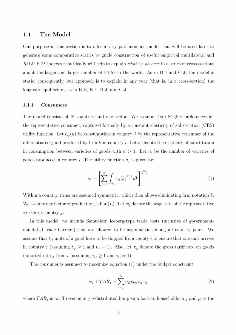
The model consists of N countries and one sector. We assume Dixit-Stiglitz preferences for

the representative consumer, captured formally by a constant elasticity of substitution (CES)

utility function. Let cij(k) be consumption in country j by the representative consumer of the

differentiated good produced by firm k in country i. Let σ denote the elasticity of substitution

in consumption between varieties of goods with σ > 1. Let ni be the number of varieties of

goods produced in country i. The utility function uj is given by:

uj =

[N∑i=1

∫ni

cij(k)σ−1σ dk

] σσ−1

. (1)

Within a country, firms are assumed symmetric, which then allows eliminating firm notation k.

We assume one factor of production, labor (L). Let wj denote the wage rate of the representative

worker in country j.

In this model, we include Samuelson iceberg-type trade costs (inclusive of government-

mandated trade barriers) that are allowed to be asymmetric among all country pairs. We

assume that tij units of a good have to be shipped from county i to ensure that one unit arrives

in country j (assuming tij ≥ 1 and tii = 1). Also, let τij denote the gross tariff rate on goods

imported into j from i (assuming τij ≥ 1 and τii = 1).

The consumer is assumed to maximize equation (1) under the budget constraint:

wj + TARj =N∑i=1

nipitijτijcij, (2)

where TARj is tariff revenue in j redistributed lump-sum back to households in j and pi is the

4

producer’s price of good g in country i. This maximization yields a set of demand equations

for national economy j with Lj households:

Xij =ni (pitijτij)

−σ∑i(ni/τij)(pitijτij)

1−σYj, (3)

where Xij is demand in country j for goods from country i and Yj denotes national income in

j. In the absence of lump-sum tariff redistributions, the term (ni/τij) in equation (3) reduces

to ni. Equation (3) shows that the model embeds “structural gravity.”

1.1.2 Firms

All firms in the industry are assumed to produce under the same technology. The output of

goods produced by a firm in country i, denoted by gi, requires li units of labor, as well as an

amount φ of fixed costs, expressed in terms of units of labor. The production function – similar

to that in Krugman (1980) – is given by:

li = φ+ gi, (4)

where we assume as traditional a constant marginal product of labor (set to unity). Firms

maximize profits subject to the technology defined in equation (4), given the demand schedule

derived in Section (1.1.1). In this model, profit maximization leads to a constant markup over

marginal production costs and there are zero profits in equilibrium due to free entry and exit.

Profit maximization ensures:

pi =σ

σ − 1wi. (5)

Zero profits in equilibrium ensure:

gi = φ (σ − 1) . (6)

5

1.1.3 Factor Endowment Constraint

We assume that endowments of labor, Li, are exogenously given and internationally immobile.

Assuming full employment, the following factor market condition holds:

Li = nili (7)

or

ni = (φσ)−1Li. (8)

The zero profit conditions and the clearing of goods and factor markets lead to balanced

multilateral trade for each economy.

1.2 Numerical Simulation: Parameter Selection

We calibrate the model for a world economy with potentially asymmetric labor endowments

and bilateral trade costs. Our model can then be simulated to motivate testable hypotheses

regarding the relative effects on the net utility gain of FTAij of FTAs of i and j with third-

countries k (own-FTA effects) and of FTAs of third-country-pairs kl (cross-FTA effects).

We calibrate the model identically to that in B-B; since the model is simpler, some pa-

rameters specified there are absent here. For the utility function, we have one parameter, the

elasticity of substitution between varieties of goods (σ). We set σ=4 as in B-B. For technol-

ogy, we set the fixed cost term in the production function to unity (φ = 1), without loss of

generality. We will discuss later the sensitivity of our results to variation in these parameters.

Initially, factor endowments of labor are assumed identical across all countries in the symmetric

benchmark equilibrium with values of Li = 100 for all countries.

The number of firms, product varieties, labor employments, wage rates, consumption levels,

and price levels in each country can be determined uniquely given the parameters of the model

(σ, φ), labor endowments, and initial transport cost and tariff rates. Following B-B, we separate

transport costs into intra-continental and inter-continental “iceberg” components. Let a denote

the portion of the good that “melts” intra-continentally and b the portion that melts inter-

continentally; hence, within continents tij = 1/(1 − a) and between countries on different

6

continents tij = [1/(1 − a)][1/(1 − b)]. We will allow both a and b to vary between their full

potential values of 0 (i.e., zero transport costs) and 1 (i.e., prohibitive transport costs) to show

sensitivity of the results to variation in transport costs.

As in B-B, we assume the existence in each country of a social planner, which sets tariff

rates (τij−1) initially at 0.3. We discuss the choice of this value in the next section. Based upon

initial parameter values, the social planner in each country considers whether its representative

consumer’s utility would be better off or worse off from forming an FTA. For a country’s planner

to form a new – or join an existing – FTA, the change in utility from doing so must be positive.

1.3 Numerical Simulation: Nash Equilibrium Tariffs and Tariff

Complementarity

The purpose of this section is to show the model is amenable to calculating Nash equilibrium

tariff rates, to rationalize setting initial tariff rates at 0.3, and to demonstrate the existence

of “tariff/FTA complementarity” in our model. As noted in B-B, the ideal approach would

be to consider the Nash equilibrium tariffs. The Nash equilibrium tariffs in a post-integration

situation are likely to differ from those in the pre-integration situation.

First, given the parameter settings just noted above, we calculate the Nash equilibrium

tariffs in the six-country case with zero intra-continental and intercontinental transport costs.

For six symmetric economies, the Nash equilibrium tariffs are approximately 0.3. Hence, for

comparative statics in subsequent sections, we set tariffs initially at 0.3.

Second, in the presence of endogenous tariffs, we can also show that the model potentially

allows for “tariff complementarity.” Bagwell and Staiger (1998) showed in a simple static model

with three symmetric economies with endogenous tariffs that when two countries (exogenously)

lower their mutual tariffs to zero (i.e., an FTA) that it is in each of their interests to lower their

external tariff to the third nonmember country. In particular, in the context of a three-country

model with each country’s import market served by competing exports from the other two,

linear demand curves (Dij = α− βPij where Dij (Pij) is quantity demanded (price) in j for i’s

product), and optimal endogenous tariffs, each of the three countries’ initial tariff rates equals

0.38β. If two countries i and j form exogenously an FTA, the post-integration Nash equilibrium

tariffs for i and j on products from ROW fall to 0.14β, or by 63 percent. Moreover, ROW ’s

tariff on products from either i or j remain unchanged at 0.38β.

7

A similar result occurs in our model. For comparison to the example above, as well as for

computational convenience, consider a three-symmetric-country version of our model (i, j, k).

In the three-country case with CES preferences, our initial Nash equilibrium tariffs are 0.4. Con-

sider an exogenous FTA between i and k, as in Bagwell and Staiger (1998). In our model, the

optimal post-integration endogenous tariff rates for countries i and k fall to less than 0.20 (de-

creasing by more than 50 percent) and the optimal tariff for j remains at 0.4. Thus, as Bagwell

and Staiger conclude, this suggests a role for FTAs being building blocs rather than stumbling

blocs toward multilateral liberalization. Moreover, this suggests for our purposes that (static)

tariff-complementarity implies – for country i – that an FTA between i and k increases the net

utility gain from i forming an FTA with j; we will call this “FTA complementarity.” Moreover,

this suggests that – in a four-country case – an exogenous FTA between k and l implies those

two countries’ external tariffs will fall, but there will be no tariff/FTA-complementarity effects

on i or j.3

1.4 Numerical Simulation: Comparative Static Results

We use the numerical version of our model to generate two new comparative statics regarding

cross-FTA and own-FTA effects. Prior to discussing those results, section 1.4.1 summarizes the

expected effects on the net utility gains of an FTA between country-pair ij (FTAij) of several

bilateral economic determinants established in Baier and Bergstrand (2004). In section 1.4.2,

we address two new comparative statics regarding the relative impacts on net utility gains of

3Such effects also hold for customs unions, with some quantitative differences. Some caveats are in orderregarding these conclusions. First, as in Bagwell and Staiger (1998, section 2), this example is nested in anon-cooperative Nash equilibrium, and thus ignores that FTAs in reality are created in a possible environmentof multilateral cooperation. Thus, we assume that there is some cost to attaining multilateral free trade, suchas enforcement of multilateral agreements. Second, Bagwell and Staiger go on to address two other effects, atariff-discrimination effect and a punishment effect, that can potentially offset the tariff-complementarity effect,and lead two FTA members to raise external tariffs. Consequently, Bagwell and Staiger (1998) suggest thatdeveloping countries that have formed FTAs might have (due to ineffective multilateral liberalization) incentivesto reduce external tariffs, whereas developed countries that have formed FTAs might have (because of moresuccessful multilateral liberalizations) incentives to raise external tariffs. Finally, Ornelas (2005c) addressesthese considerations allowing for endogenous external tariffs and FTAs and political economy considerations,and argues that FTAs tend to induce members’ governments to reduce external tariffs. Ornelas introduces twoeffects that suggest FTAs will tend to promote reductions in members’ external tariffs and further liberalizationmultilaterally. One effect, a “strategic effect,” reflects the weakening of the “profit-sharing” motive for protectionwhen two countries form an FTA. Since partners’ firms capture free access to the home market, they capturethat market share taken away from outside firms, reducing incentives for the FTA members’ governments toraise external tariffs. Ornelas’ other effect is a “distributive” one. The formation of an FTA shifts home marketshares from domestic firms to members’ counterparts, reducing the ability of FTA governments to shift surplusfrom consumers to producers through higher external tariffs. This creates a channel for FTA governments tolower external tariffs. See Freund and Ornelas (2009) for an excellent survey on these issues.

8

FTAij of cross-FTA and own-FTA effects in the context of a Krugman-type model. Following

B-B, initially we assume three continents (1, 2, 3) with two countries on each continent (A,B).4

1.4.1 Established Bilateral Economic Determinants

This section summarizes the effects of several “core” economic variables influencing the net

utility gains for countries i and j of FTAij as established in B-B. The rationale is to justify

including these core variables later in our empirical specifications. See B-B for details.5

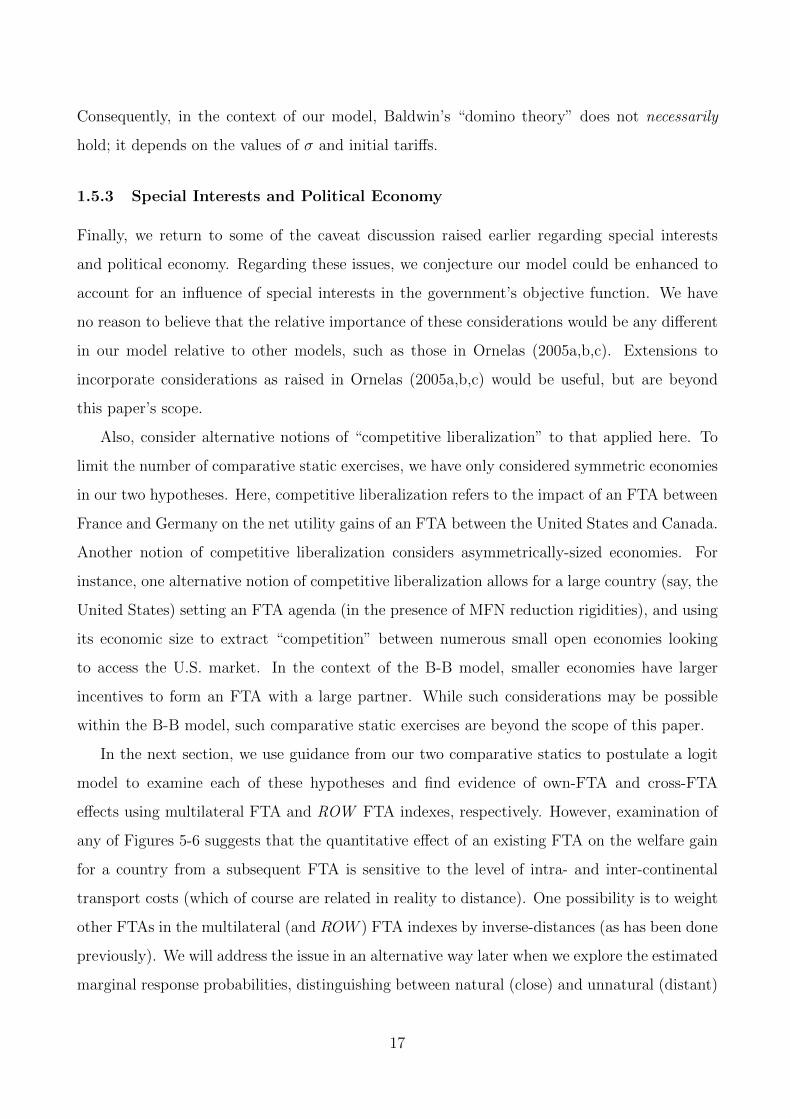
One of the key implications from Krugman (1991a,b), Frankel, Stein, and Wei (1995),

Frankel (1997), and B-B is that natural (intra-continental) FTAs are unambiguously welfare

superior to unnatural (inter-continental) FTAs; hence, two countries’ social planners are more

likely to form an FTA the smaller the distance between them (and if they share the same

continent). For a given distance between a country-pair and ROW , the closer are two countries,

the lower their transport costs and consequently the higher their trade volume. Elimination

of the ad valorem tariff between close FTA members alleviates the price distortion on a large

amount of trade, improving real income and utility of consumers more in intra-continental

FTAs, as shown in Figure 1. In this class of models, all trade volume increases are at the

intensive margin.6

The utility gain from an FTA between two countries increases as both countries’ economic

sizes increase proportionately (holding constant their relative size). In Figure 1, all countries

are equivalently sized in labor (and GDP). As in B-B, consider asymmetric sizes in terms of

absolute factor endowments to determine the scale-economies cum taste-for-variety effects. For

brevity, we limit our comparative statics to natural trade partners only. We allow countries on

continent 1 (1A, 1B) to have larger absolute endowments of labor than countries on continent

2 (2A, 2B), and 2A and 2B to have larger absolute endowments than countries on continent 3

(3A, 3B); however, for any country-pair on the same continent, GDPs are identical. As above,

we consider a single FTA between a pair of countries on one continent (different from B-B).

4A “visualization” of the “world” is shown in Figure 4, to be discussed later.5The reader familiar with B-B may skip this section.6The model assumes homogeneous productivities across firms in a country, as addressed earlier in section

1. There are other approaches as well to suggest why FTAs tend to be formed among closer, rather thandistant, countries. Zissimos (2009), for instance, adapts the model of Yi (1996) to show that – since morerents are dissipated through transportation between regions rather than within them – regional FTAs eliminatethe greater harmful “rent-shifting” among members and also has greater beneficial terms-of-trade effects. Thisreduction of harmful “rent-shifting” pushes countries more toward forming regional FTAs.

9

Figure 2 presents two surfaces, with the top one illustrating the welfare gain for either country

1A or 1B of an FTA between large economies 1A and 1B and the bottom surface illustrating

the gain for either country 3A or 3B of an FTA between small economies 3A and 3B. We

emphasize two results. First, an FTA between two small economies is still welfare-improving.

This result differs from that in Figure 2 of B-B where all natural partners went into an FTA

simultaneously. With only one agreement at a time, even small countries can benefit from

a bilateral FTA; hence, the trade-creation effect dominates the trade-diversion effect. This

comparative-static result – that small countries can benefit on net from FTAs on the same

continent – is new. Second, as in B-B, large countries benefit more than small countries from

FTAs. Intuitively, welfare gains from an FTA should be higher for countries with larger absolute

factor endowments (and thus larger real GDPs) due to reducing price distortions on a larger

set of goods. An FTA between two large partners (1A, 1B) increases the volume of trade (at

the intensive margin) in more varieties than an FTA between two small partners (3A, 3B) and

reduces trade in fewer varieties from nonmembers than two small partners would, improving

utility more among two large countries relative to that among two small countries. Also, the

consequent larger increase in trade among two large economies from a bilateral FTA causes a

larger net expansion of demand and hence a larger rise in real income (and terms of trade).

Small countries 3A and 3B face considerable trade diversion when 1A and 1B form an FTA;

the fall in relative demand for the small countries’ production causes an erosion of terms of

trade.

The utility gain from an FTA between two countries increases the more similar their eco-

nomic sizes (for a given total real GDP of the country-pair). In this class of models, the more

similar are the real GDPs of two countries on the same continent the larger the welfare gains

from an FTA, for a given total GDP of the pair. In the previous comparative static, countries

on the same continent had identical economic sizes. If 1A and 1B have identical shares of the

two countries’ factor endowments, the formation of an FTA provides gains from an increase

in the volume of trade (at the intensive margin) as the tariff distortion is eliminated on much

trade. By contrast, if 1A has virtually all of the labor on continent 1, formation of an FTA

provides little welfare increase, since there is virtually no trade between 1A and 1B because 1B

produces few varieties. Figure 3 illustrates this. The top surface shows the welfare gain for 1A

when 1A and 1B are identically sized. The bottom surface shows the welfare gain for 1A when

10

it has a larger share of the continent’s labor force. Since 1A is larger, it gains less from an FTA

with 1B. This result was found already in B-B, but we present it here for completeness.

1.4.2 Cross-FTA and Own-FTA Effects

The following two hypotheses (Hypotheses 1 and 2 ) address the effects of existing FTAs on

the welfare gains of subsequent FTAs. It is important to note, however, that our model is a

static one (a single period), so there is no formal sense of “time.” The model can, however,

generate numerical welfare effects of an FTA between a country-pair conditioned upon various

alternative scenarios, such as an FTA or no FTA between another country-pair. It is in this

manner we use our model’s comparative statics to motivate for the empirical analysis later

of a series of cross-sections how existing FTAs influence the likelihood of FTAs in subsequent

years. In order to “hold constant” as many effects as possible in our nonlinear model, we re-

sume the assumption that all countries have identical absolute factor endowments, to eliminate

asymmetries in economic size.

As suggested earlier, the two hypotheses are distinguished because Hypothesis 1 addresses

cross-FTA effects and Hypothesis 2 addresses own-FTA effects. Figures 4a and 4b illustrate the

two hypotheses, 1 and 2, respectively. Figure 4a illustrates the case of two countries, 1A and 1B

– say, the United States and Mexico – forming an FTA conditioned upon two other countries, 2A

and 2B – say, France and Germany – already having an FTA. By contrast, Figure 4b illustrates

the case of two countries, 1A and 1B – say, the United States and Mexico – forming an FTA

conditioned upon one of the countries, 1A (say, the United States), already having an agreement

with another country, 2A (say, Canada). It is important to note that – while countries 2A and

2B represent two countries on different continents – our framework allows inter- and intra-

continental transport costs to vary between zero and prohibitive. Moreover, most models

discussing potential trade diversion, terms-of-trade impacts, and tariff-complementarity effects

omit natural trade costs.

Hypothesis 1 (Cross-FTA): The utility gain from an FTA between two countries 1A and

1B increases due to an existing FTA between two other countries – on the same or different

continents – due to potential trade diversion, trade creation, and terms-of-trade effects.

We consider first the case of two countries 1A and 1B forming a bilateral FTA; we assume

that all six countries initially have a tariff rate of 30 percent on each others’ products, as

11

discussed earlier.7 We know from earlier comparative statics (Figure 1) that – conditioned

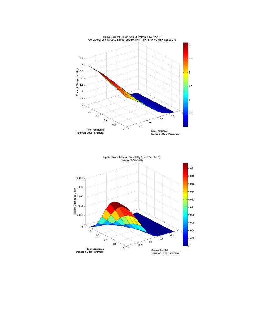
upon no other FTAs in existence – such an FTA is necessarily welfare-improving. Figure 5a

actually illustrates two surfaces. The bottom surface is the welfare gain for 1A of an FTA

between countries 1A and 1B and no other FTA existing among all countries; we denote this

FTA1A,1B.

Suppose now instead that 2A and 2B already have an FTA. Figure 5a also illustrates the

welfare gain to 1A of the formation of an FTA with 1B conditioned on an existing agreement

between 2A and 2B; this is the top surface. While the two surfaces are similar, the existence

of FTA2A,2B increases unambiguously the gain in welfare of an FTA between 1A and 1B. This

is confirmed in Figure 5b which shows the (vertical) difference between the two surfaces, that

is, the gains to 1A from an FTA between 1A and 1B conditioned on FTA2A,2B less the gains

to 1A from FTA1A,1B without conditioning. Figure 5b reveals that the gain to 1A’s utility

of FTA1A,1B attributable to FTA2A,2B is positive for all possible intra- and inter-continental

transports costs (from zero to prohibitive), given initial tariffs of 30 percent and σ = 4. This

figure suggests that country 1A’s (and, by symmetry, 1B’s) “demand for membership” in an

FTA with country 1B (1A) will tend to be higher if 2A and 2B have an existing FTA. The

positive difference is the role of “third-country-pairs” creating competitive liberalization.8

Intuitively, when 2A and 2B form an FTA, each of 1A and 1B experience trade diversion,

a loss of terms of trade, and erosion in real income. When a country pair (2A, 2B) is remote –

that is, when b is large – there are negligible volume-of-trade and terms-of-trade (real income)

effects on 1A’s utility from the formation of FTA2A,2B because there is little trade to be diverted

between country 1A and countries 2A and 2B. However, if inter- (and intra-) continental trade

costs are low, then 1A trades considerably with 2A and 2B; an FTA between 2A and 2B

causes substantive trade diversion for 1A, eroding 1A’s volume of trade with 2A and 2B and

1A’s utility and real income, but improving 1A’s volume of trade with 1B. Consequently, the

formation of FTA1A,1B has an even larger impact on 1A’s utility – in the presence of FTA2A,2B

than in its absence – because the elimination of tariffs from FTA1A,1B on the greater volume

of trade between 1A and 1B due to FTA2A,2B more than offsets the terms-of-trade loss due

to trade diversion from FTA2A,2B. FTA2A,2B effectively has made countries 1A and 1B more

7In the next section’s sensitivity analysis, we examine the robustness of these comparative statics to otherinitial tariff levels.

8The comparative-static effect is qualitatively identical if the other FTA is between two countries on anothercontinent (3A, 3B).

12

“economically remote” and this isolation has made 1A and 1B economically more natural trade

partners, enhancing the gains from an FTA. We note now that, at low transport costs, the net

utility gain for 1A (and, by symmetry, 1B) is at most 0.02 of one percent. We will discuss the

sensitivity of the results to alternative values of σ, φ, and initial tariff rates later.

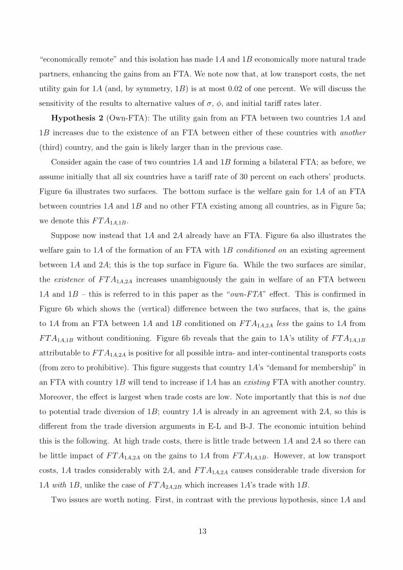
Hypothesis 2 (Own-FTA): The utility gain from an FTA between two countries 1A and

1B increases due to the existence of an FTA between either of these countries with another

(third) country, and the gain is likely larger than in the previous case.

Consider again the case of two countries 1A and 1B forming a bilateral FTA; as before, we

assume initially that all six countries have a tariff rate of 30 percent on each others’ products.

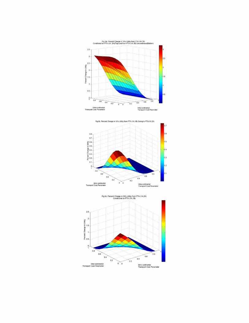
Figure 6a illustrates two surfaces. The bottom surface is the welfare gain for 1A of an FTA

between countries 1A and 1B and no other FTA existing among all countries, as in Figure 5a;

we denote this FTA1A,1B.

Suppose now instead that 1A and 2A already have an FTA. Figure 6a also illustrates the

welfare gain to 1A of the formation of an FTA with 1B conditioned on an existing agreement

between 1A and 2A; this is the top surface in Figure 6a. While the two surfaces are similar,

the existence of FTA1A,2A increases unambiguously the gain in welfare of an FTA between

1A and 1B – this is referred to in this paper as the “own-FTA” effect. This is confirmed in

Figure 6b which shows the (vertical) difference between the two surfaces, that is, the gains

to 1A from an FTA between 1A and 1B conditioned on FTA1A,2A less the gains to 1A from

FTA1A,1B without conditioning. Figure 6b reveals that the gain to 1A’s utility of FTA1A,1B

attributable to FTA1A,2A is positive for all possible intra- and inter-continental transports costs

(from zero to prohibitive). This figure suggests that country 1A’s “demand for membership” in

an FTA with country 1B will tend to increase if 1A has an existing FTA with another country.

Moreover, the effect is largest when trade costs are low. Note importantly that this is not due

to potential trade diversion of 1B; country 1A is already in an agreement with 2A, so this is

different from the trade diversion arguments in E-L and B-J. The economic intuition behind

this is the following. At high trade costs, there is little trade between 1A and 2A so there can

be little impact of FTA1A,2A on the gains to 1A from FTA1A,1B. However, at low transport

costs, 1A trades considerably with 2A, and FTA1A,2A causes considerable trade diversion for

1A with 1B, unlike the case of FTA2A,2B which increases 1A’s trade with 1B.

Two issues are worth noting. First, in contrast with the previous hypothesis, since 1A and

13

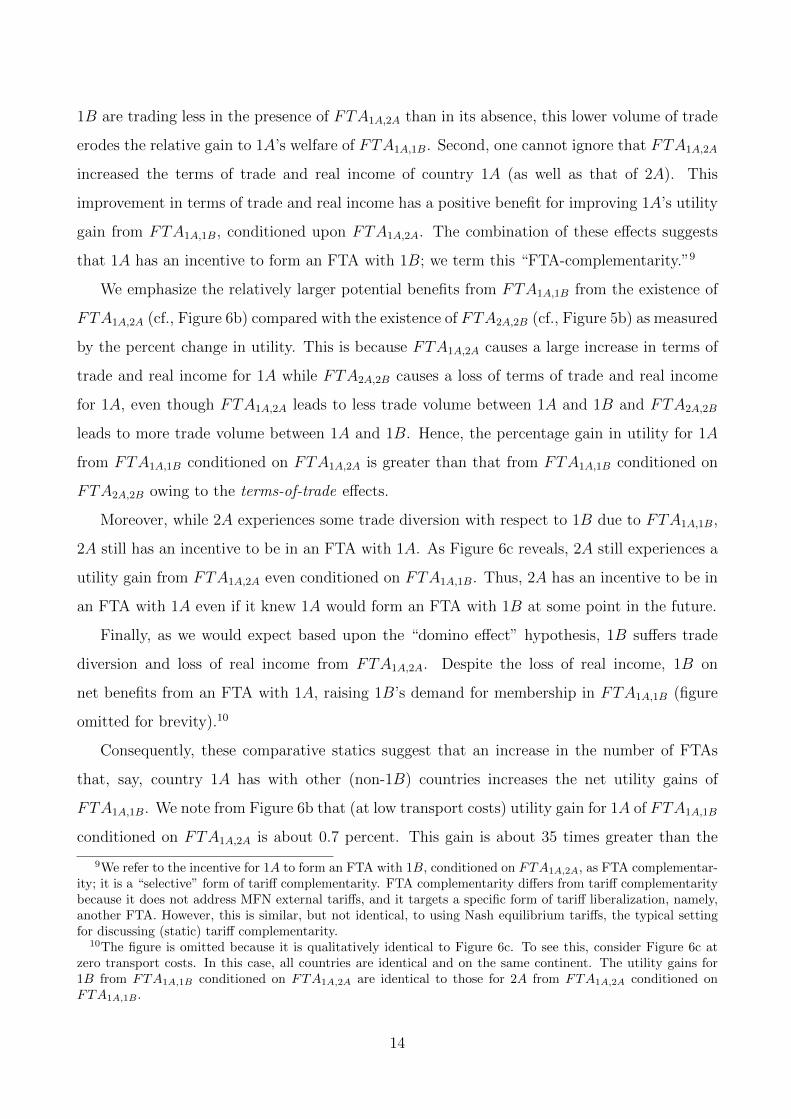
1B are trading less in the presence of FTA1A,2A than in its absence, this lower volume of trade

erodes the relative gain to 1A’s welfare of FTA1A,1B. Second, one cannot ignore that FTA1A,2A

increased the terms of trade and real income of country 1A (as well as that of 2A). This

improvement in terms of trade and real income has a positive benefit for improving 1A’s utility

gain from FTA1A,1B, conditioned upon FTA1A,2A. The combination of these effects suggests

that 1A has an incentive to form an FTA with 1B; we term this “FTA-complementarity.”9

We emphasize the relatively larger potential benefits from FTA1A,1B from the existence of

FTA1A,2A (cf., Figure 6b) compared with the existence of FTA2A,2B (cf., Figure 5b) as measured

by the percent change in utility. This is because FTA1A,2A causes a large increase in terms of

trade and real income for 1A while FTA2A,2B causes a loss of terms of trade and real income

for 1A, even though FTA1A,2A leads to less trade volume between 1A and 1B and FTA2A,2B

leads to more trade volume between 1A and 1B. Hence, the percentage gain in utility for 1A

from FTA1A,1B conditioned on FTA1A,2A is greater than that from FTA1A,1B conditioned on

FTA2A,2B owing to the terms-of-trade effects.

Moreover, while 2A experiences some trade diversion with respect to 1B due to FTA1A,1B,

2A still has an incentive to be in an FTA with 1A. As Figure 6c reveals, 2A still experiences a

utility gain from FTA1A,2A even conditioned on FTA1A,1B. Thus, 2A has an incentive to be in

an FTA with 1A even if it knew 1A would form an FTA with 1B at some point in the future.

Finally, as we would expect based upon the “domino effect” hypothesis, 1B suffers trade

diversion and loss of real income from FTA1A,2A. Despite the loss of real income, 1B on

net benefits from an FTA with 1A, raising 1B’s demand for membership in FTA1A,1B (figure

omitted for brevity).10

Consequently, these comparative statics suggest that an increase in the number of FTAs

that, say, country 1A has with other (non-1B) countries increases the net utility gains of

FTA1A,1B. We note from Figure 6b that (at low transport costs) utility gain for 1A of FTA1A,1B

conditioned on FTA1A,2A is about 0.7 percent. This gain is about 35 times greater than the

9We refer to the incentive for 1A to form an FTA with 1B, conditioned on FTA1A,2A, as FTA complementar-ity; it is a “selective” form of tariff complementarity. FTA complementarity differs from tariff complementaritybecause it does not address MFN external tariffs, and it targets a specific form of tariff liberalization, namely,another FTA. However, this is similar, but not identical, to using Nash equilibrium tariffs, the typical settingfor discussing (static) tariff complementarity.

10The figure is omitted because it is qualitatively identical to Figure 6c. To see this, consider Figure 6c atzero transport costs. In this case, all countries are identical and on the same continent. The utility gains for1B from FTA1A,1B conditioned on FTA1A,2A are identical to those for 2A from FTA1A,2A conditioned onFTA1A,1B .

14

gain to 1A of FTA1A,1B conditioned on FTA2A,2B, cf., Figure 5b, which was at most 0.02

percent. These relative values suggest that marginal own-FTA effects may well dwarf marginal

cross-FTA effects in our empirical analysis later. However, before that, we discuss in the next

section the robustness of these comparative statics to several considerations.

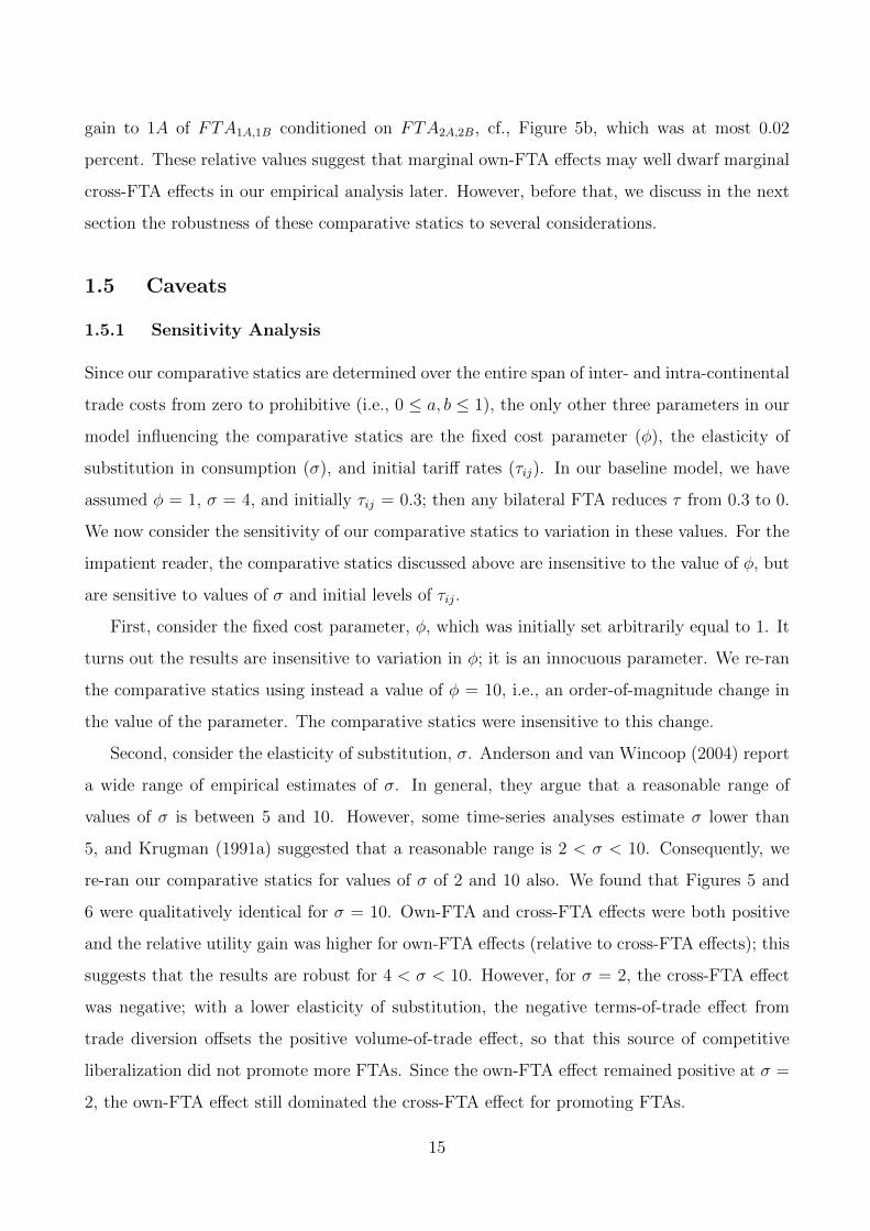
1.5 Caveats

1.5.1 Sensitivity Analysis

Since our comparative statics are determined over the entire span of inter- and intra-continental

trade costs from zero to prohibitive (i.e., 0 ≤ a, b ≤ 1), the only other three parameters in our

model influencing the comparative statics are the fixed cost parameter (φ), the elasticity of

substitution in consumption (σ), and initial tariff rates (τij). In our baseline model, we have

assumed φ = 1, σ = 4, and initially τij = 0.3; then any bilateral FTA reduces τ from 0.3 to 0.

We now consider the sensitivity of our comparative statics to variation in these values. For the

impatient reader, the comparative statics discussed above are insensitive to the value of φ, but

are sensitive to values of σ and initial levels of τij.

First, consider the fixed cost parameter, φ, which was initially set arbitrarily equal to 1. It

turns out the results are insensitive to variation in φ; it is an innocuous parameter. We re-ran

the comparative statics using instead a value of φ = 10, i.e., an order-of-magnitude change in

the value of the parameter. The comparative statics were insensitive to this change.

Second, consider the elasticity of substitution, σ. Anderson and van Wincoop (2004) report

a wide range of empirical estimates of σ. In general, they argue that a reasonable range of

values of σ is between 5 and 10. However, some time-series analyses estimate σ lower than

5, and Krugman (1991a) suggested that a reasonable range is 2 < σ < 10. Consequently, we

re-ran our comparative statics for values of σ of 2 and 10 also. We found that Figures 5 and

6 were qualitatively identical for σ = 10. Own-FTA and cross-FTA effects were both positive

and the relative utility gain was higher for own-FTA effects (relative to cross-FTA effects); this

suggests that the results are robust for 4 < σ < 10. However, for σ = 2, the cross-FTA effect

was negative; with a lower elasticity of substitution, the negative terms-of-trade effect from

trade diversion offsets the positive volume-of-trade effect, so that this source of competitive

liberalization did not promote more FTAs. Since the own-FTA effect remained positive at σ =

2, the own-FTA effect still dominated the cross-FTA effect for promoting FTAs.

15

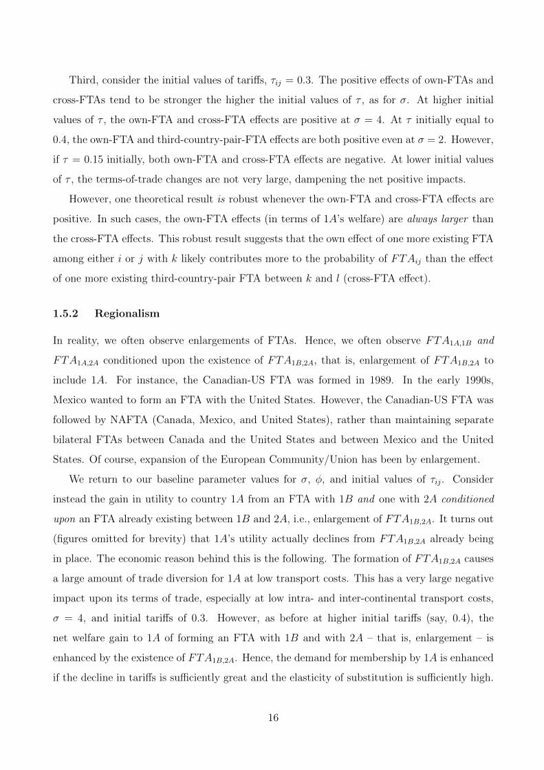
Third, consider the initial values of tariffs, τij = 0.3. The positive effects of own-FTAs and

cross-FTAs tend to be stronger the higher the initial values of τ , as for σ. At higher initial

values of τ , the own-FTA and cross-FTA effects are positive at σ = 4. At τ initially equal to

0.4, the own-FTA and third-country-pair-FTA effects are both positive even at σ = 2. However,

if τ = 0.15 initially, both own-FTA and cross-FTA effects are negative. At lower initial values

of τ , the terms-of-trade changes are not very large, dampening the net positive impacts.

However, one theoretical result is robust whenever the own-FTA and cross-FTA effects are

positive. In such cases, the own-FTA effects (in terms of 1A’s welfare) are always larger than

the cross-FTA effects. This robust result suggests that the own effect of one more existing FTA

among either i or j with k likely contributes more to the probability of FTAij than the effect

of one more existing third-country-pair FTA between k and l (cross-FTA effect).

1.5.2 Regionalism

In reality, we often observe enlargements of FTAs. Hence, we often observe FTA1A,1B and

FTA1A,2A conditioned upon the existence of FTA1B,2A, that is, enlargement of FTA1B,2A to

include 1A. For instance, the Canadian-US FTA was formed in 1989. In the early 1990s,

Mexico wanted to form an FTA with the United States. However, the Canadian-US FTA was

followed by NAFTA (Canada, Mexico, and United States), rather than maintaining separate

bilateral FTAs between Canada and the United States and between Mexico and the United

States. Of course, expansion of the European Community/Union has been by enlargement.

We return to our baseline parameter values for σ, φ, and initial values of τij. Consider

instead the gain in utility to country 1A from an FTA with 1B and one with 2A conditioned

upon an FTA already existing between 1B and 2A, i.e., enlargement of FTA1B,2A. It turns out

(figures omitted for brevity) that 1A’s utility actually declines from FTA1B,2A already being

in place. The economic reason behind this is the following. The formation of FTA1B,2A causes

a large amount of trade diversion for 1A at low transport costs. This has a very large negative

impact upon its terms of trade, especially at low intra- and inter-continental transport costs,

σ = 4, and initial tariffs of 0.3. However, as before at higher initial tariffs (say, 0.4), the

net welfare gain to 1A of forming an FTA with 1B and with 2A – that is, enlargement – is

enhanced by the existence of FTA1B,2A. Hence, the demand for membership by 1A is enhanced

if the decline in tariffs is sufficiently great and the elasticity of substitution is sufficiently high.

16

Consequently, in the context of our model, Baldwin’s “domino theory” does not necessarily

hold; it depends on the values of σ and initial tariffs.

1.5.3 Special Interests and Political Economy

Finally, we return to some of the caveat discussion raised earlier regarding special interests

and political economy. Regarding these issues, we conjecture our model could be enhanced to

account for an influence of special interests in the government’s objective function. We have

no reason to believe that the relative importance of these considerations would be any different

in our model relative to other models, such as those in Ornelas (2005a,b,c). Extensions to

incorporate considerations as raised in Ornelas (2005a,b,c) would be useful, but are beyond

this paper’s scope.

Also, consider alternative notions of “competitive liberalization” to that applied here. To

limit the number of comparative static exercises, we have only considered symmetric economies

in our two hypotheses. Here, competitive liberalization refers to the impact of an FTA between

France and Germany on the net utility gains of an FTA between the United States and Canada.

Another notion of competitive liberalization considers asymmetrically-sized economies. For

instance, one alternative notion of competitive liberalization allows for a large country (say, the

United States) setting an FTA agenda (in the presence of MFN reduction rigidities), and using

its economic size to extract “competition” between numerous small open economies looking

to access the U.S. market. In the context of the B-B model, smaller economies have larger

incentives to form an FTA with a large partner. While such considerations may be possible

within the B-B model, such comparative static exercises are beyond the scope of this paper.

In the next section, we use guidance from our two comparative statics to postulate a logit

model to examine each of these hypotheses and find evidence of own-FTA and cross-FTA

effects using multilateral FTA and ROW FTA indexes, respectively. However, examination of

any of Figures 5-6 suggests that the quantitative effect of an existing FTA on the welfare gain

for a country from a subsequent FTA is sensitive to the level of intra- and inter-continental

transport costs (which of course are related in reality to distance). One possibility is to weight

other FTAs in the multilateral (and ROW ) FTA indexes by inverse-distances (as has been done

previously). We will address the issue in an alternative way later when we explore the estimated

marginal response probabilities, distinguishing between natural (close) and unnatural (distant)

17

FTA partners.

18

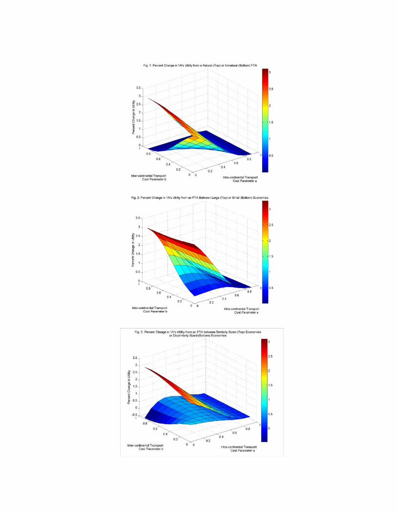
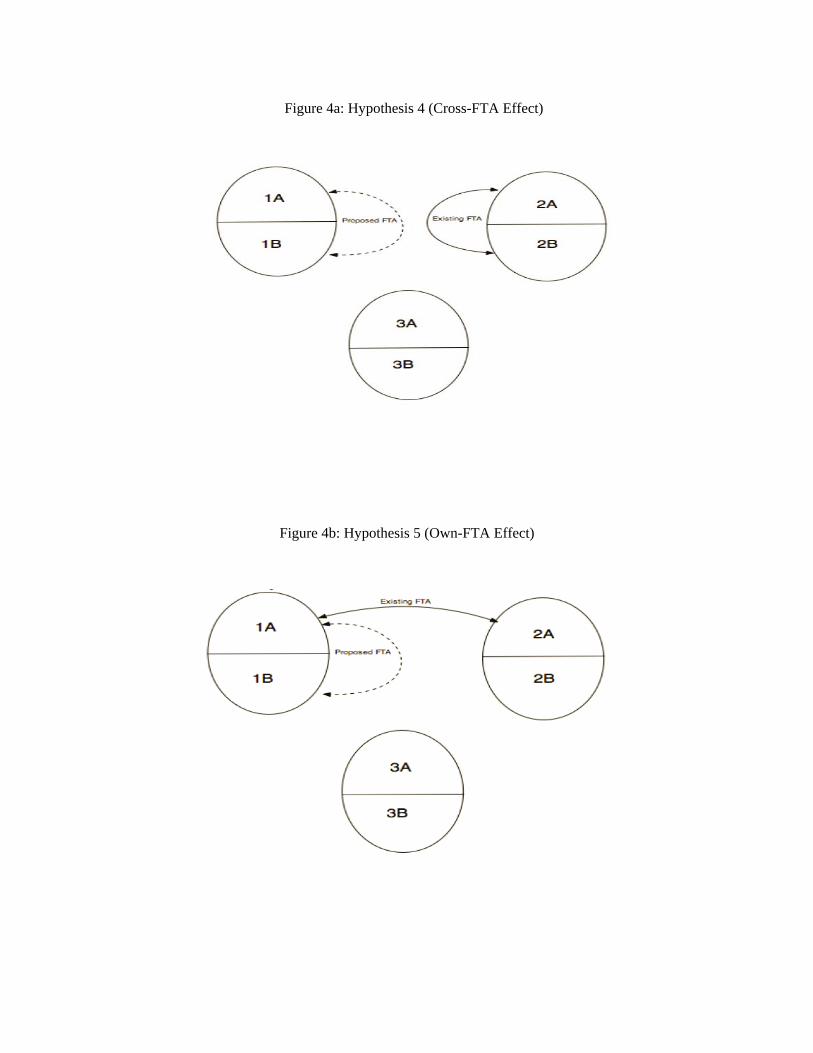
Figure 4a: Hypothesis 4 (Cross-FTA Effect)

Figure 4b: Hypothesis 5 (Own-FTA Effect)