2016 Line haul Locomotive Model & Update

California Air Resources BoardOff Road Diesel Analysis Section

October 2017

1

2

Table of Contents1. Introduction..................................................................................................................................4

2. Background..................................................................................................................................4

3. New Engine Standards and Remanufacturing Locomotives.......................................................5

4. Inputs and Calculations................................................................................................................6

4.1. Population and Tier Distribution...........................................................................................6

4.2. Horsepower Distribution and Projection...............................................................................6

4.3. Activity..................................................................................................................................8

4.3.1. Methodology 1: Activity by Reported Locomotive Duty Cycle....................................9

4.3.2. Methodology 2: Activity by Reported Gross Ton-Miles.............................................10

4.3.3. Methodology 3: Activity by Estimated Locomotive-Hours.........................................12

4.4. Growth................................................................................................................................14

4.5. Emission Factors.................................................................................................................16

4.5.1. Emission Adjustments..................................................................................................17

4.6. Spatial and Temporal Allocation........................................................................................18

5. Turnover and Rule Analysis......................................................................................................21

5.1. Baseline Natural Turnover..................................................................................................21

5.2. Fleet Sales...........................................................................................................................22

6. Emission Results........................................................................................................................24

7. Validation and Quality Assurance.............................................................................................29

8. South Coast and Statewide Emissions Results..........................................................................30

3

Table 3-1: Locomotive Tier and Emissions Factors........................................................................5Table 4-1 2011 Locomotive Tier distributions across the South Coast and rest of California.......6Table 4-3 Subdivisions using Methodology 1.................................................................................9Table 4-4 Sample throttle notch data...............................................................................................9Table 4-5 Estimated grades for selected major subdivisions.........................................................11Table 4-6 Remaining subdivision activity estimated using external sources................................13Table 4-7 FAF Rail Growth Rates by Area of California.............................................................14Table 4-8 U.S. EPA Line-haul emission factors (g/bhp-hr)..........................................................16Table 4-9 U.S. EPA emission factors, measured in g/gal..............................................................17Table 4-10 Comparison of constant and grade-based allocation...................................................20Table 4-11 The 2011 estimated fuel burn for select California air basins.....................................21Table 6-1 NOx, PM, and Fuel for Selected Year..........................................................................29Table 8-1 Emissions Results for South Coast and statewide.........................................................30

Figure 3.1 Engine size of GE locomotives, 1940-2010...................................................................8Figure 3.2 Engine size of EMD locomotives, 1940-2010...............................................................9Figure 3.3 Elevation profile of the eastbound Roseville subdivision............................................13Figure 3.4 Locomotive Activity Growth.......................................................................................16Figure 3.5: Locomotive Fuel Growth Comparison........................................................................17Figure 3.6 California Air Basins....................................................................................................19Figure 3.7 Cajon northbound comparison of fuel allocation between the constant and grade-based methodologies......................................................................................................................20Figure 3.8 Cajon southbound comparison of fuel allocation between the constant and grade-based methodologies......................................................................................................................21Figure 4.1 Locomotive Survival Curve / Life-cycle......................................................................23Figure 4.2 Projected and Back-Casted Locomotive Sales.............................................................24Figure 4.3 Age distribution for Calendar Years 2016 and 2040....................................................25Figure 5.1 2016 Model Tier Distribution, South Coast MOU.......................................................26Figure 5.2 2016 Model Tier Distribution, outside the South Coast...............................................27Figure 5.3 South Coast NOx..........................................................................................................28Figure 5.4 South Coast PM............................................................................................................28Figure 5.5 California statewide NOx.............................................................................................29Figure 5.6 California statewide PM...............................................................................................29Figure 6.1 2011 South Coast and rest of California Tier comparisons.........................................30Figure 6.2 2014 South Coast and rest of California Tier comparisons.........................................31

4

1. INTRODUCTION

The Class I line-haul locomotive emissions inventory includes locomotives operating in California that provide interstate freight transportation for containers, liquid material, or bulk material. Union Pacific (UP) and Burlington Northern Santa Fe (BNSF) railroads, the two main Class I rail companies in California, supplied 2011 statewide fuel use and locomotive engine tier distribution, which was supplemented by 2014 locomotive activity specifically in the South Coast Air Basin of California, for creation of the California Air Resources Board 2016 Line-haul Locomotive emissions inventory. This report discusses calculations associated with locomotive population, activity, growth rate, model year distribution, survival curve, and benefits achieved by the 1998 Memorandum of Understanding (MOU) between the California Air Resources Board (ARB) and UP and BNSF railroads.

2. BACKGROUND

The locomotive emission inventory is broken into three main sectors: Class I freight railroads, Class III railroads, and passenger rail. Class I railroads are defined as line-haul freight railroads with 2014 revenues greater than $476 million1. Conversely, Class III (short line) locomotives move goods regionally, have lower revenues, and generally have older locomotives. This Class I Line haul locomotive inventory report does not cover or represent Class III or passenger rail. Class I locomotives emit about 80% of NOx and 79% of PM produced by all locomotives in California.

The 2016 line-haul locomotive model update uses 2011 and 2014 rail data outlining locomotive activity in the South Coast Air Basin of California, supplied by UP and BNSF railroads, the two main rail companies in California. Revisions to the 2011 locomotive inventory include updating the population, activity, growth rate, model year distribution, survival curve, and benefits achieved by the 1998 MOU. The South Coast rail data for 2014 operations was used to calibrate the model and to project locomotive activity for the entire state.

In 1998, ARB collaborated with the California railroads to create an MOU that lead to increased adoption of cleaner locomotives in the South Coast region. The MOU, together with the locomotive emission standards, brings the South Coast locomotive fleet to a Tier 2 average by 2010. On average, locomotives in the South Coast are about 1 year newer than locomotives in the rest of California, which has an average age of 6.5 years.

To verify Fleet Average Targets in the MOU are being met, UP and BNSF must track locomotive usage entering and leaving the South Coast Nonattainment Area by recording megawatt-hours (MW-hr), fuel consumption that converts to MW-hr, or fuel data, and report that information to ARB. Transponders located at or near the nonattainment borders track 1 https://www.aar.org/BackgroundPapers/Overview of America's Freight RRs.pdf

5

locomotives. This emissions inventory model used 1998 MOU data from UP and BNSF, collected in 2011 and 2014.

As part of a 2005 agreement2, UP and BNSF agreed to several conditions to reduce emissions beyond the agreement in the 1998 MOU. As stated in the agreement, railroads will minimize idling time by phasing out non-essential idling and install idling reduction devices. Railroads must promptly repair locomotives producing excessive smoke and certify a minimum of 99% of the locomotives operating within California pass smoke inspections. Furthermore, locomotives have adopted ultra-low sulfur (15 ppm) diesel fuel beginning in 2012.

3. NEW ENGINE STANDARDS AND REMANUFACTURING LOCOMOTIVES

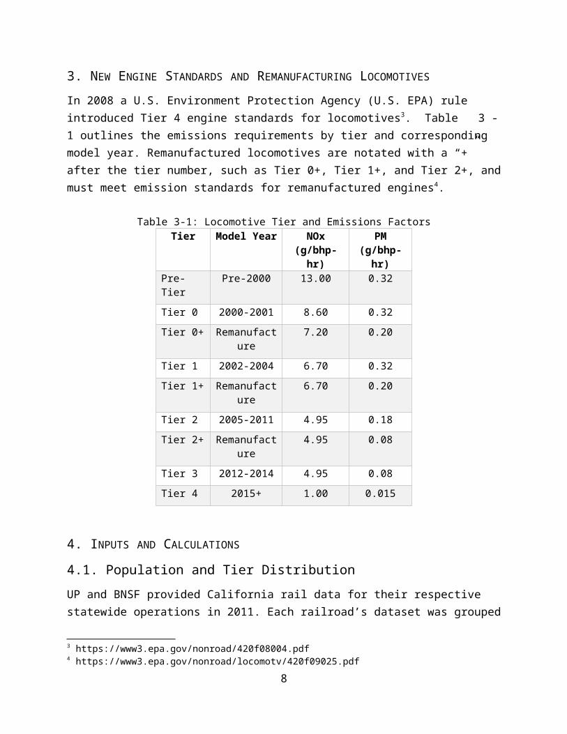
In 2008 a U.S. Environment Protection Agency (U.S. EPA) rule introduced Tier 4 engine standards for locomotives3. Table 3-1 outlines the emissions requirements by tier and corresponding model year. Remanufactured locomotives are notated with a “+” after the tier number, such as Tier 0+, Tier 1+, and Tier 2+, and must meet emission standards for remanufactured engines4.

Table 3-1: Locomotive Tier and Emissions FactorsTier Model Year NOx

(g/bhp-hr)PM

(g/bhp-hr)Pre-Tier Pre-2000 13.00 0.32

Tier 0 2000-2001 8.60 0.32

Tier 0+ Remanufacture 7.20 0.20

Tier 1 2002-2004 6.70 0.32

Tier 1+ Remanufacture 6.70 0.20

Tier 2 2005-2011 4.95 0.18

Tier 2+ Remanufacture 4.95 0.08

Tier 3 2012-2014 4.95 0.08

Tier 4 2015+ 1.00 0.015

4. INPUTS AND CALCULATIONS

4.1. Population and Tier Distribution

UP and BNSF provided California rail data for their respective statewide operations in 2011. Each railroad’s dataset was grouped according to the origin and destination of the rail line (rail

2 https://www.arb.ca.gov/railyard/ryagreement/080805fs.pdf3 https://www3.epa.gov/nonroad/420f08004.pdf4 https://www3.epa.gov/nonroad/locomotv/420f09025.pdf

6

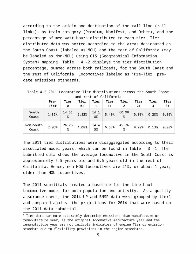
links), by train category (Premium, Manifest, and Other), and the percentage of megawatt-hours distributed to each tier. Tier-distributed data was sorted according to the areas designated as the South Coast (labeled as MOU) and the rest of California (may be labeled as Non-MOU) using GIS (Geographical Information System) mapping. Table 4-2 displays the tier distribution percentage, summed across both railroads, for the South Coast and the rest of California. Locomotives labeled as “Pre-Tier” pre-date emissions standards.

Table 4-2 2011 Locomotive Tier distributions across the South Coast and rest of CaliforniaPre-Tier Tier 0 Tier 0+ Tier 1 Tier 1+ Tier 2 Tier 2+ Tier 3 Tier 3+

South Coast 1.81% 14.51% 2.82% 14.18% 5.40% 60.98% 0.00% 0.28% 0.00%

Non-South Coast 2.95% 26.26% 4.08% 14.45

% 6.57% 45.26% 0.00% 0.13% 0.00%

The 2011 tier distributions were disaggregated according to their associated model years, which can be found in Table 3-1. The submitted data shows the average locomotive in the South Coast is approximately 5.5 years old and 6.6 years old in the rest of California. Hence, non-MOU locomotives are 21%, or about 1 year, older than MOU locomotives.

The 2011 submittals created a baseline for the Line haul Locomotive model for both population and activity. As a quality assurance check, the 2014 UP and BNSF data were grouped by tier5, and compared against the projections for 2014 that were based on the 2011 data submittal.

4.2. Horsepower Distribution and Projection

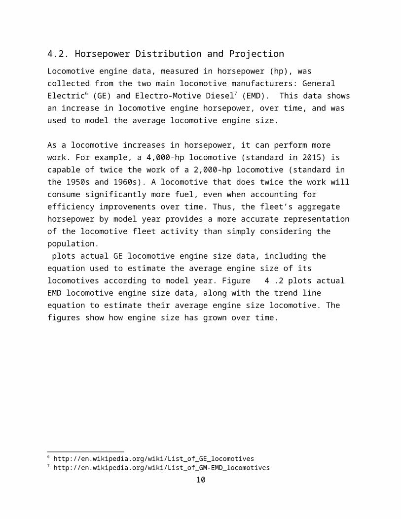
Locomotive engine data, measured in horsepower (hp), was collected from the two main locomotive manufacturers: General Electric6 (GE) and Electro-Motive Diesel7 (EMD). This data shows an increase in locomotive engine horsepower, over time, and was used to model the average locomotive engine size.

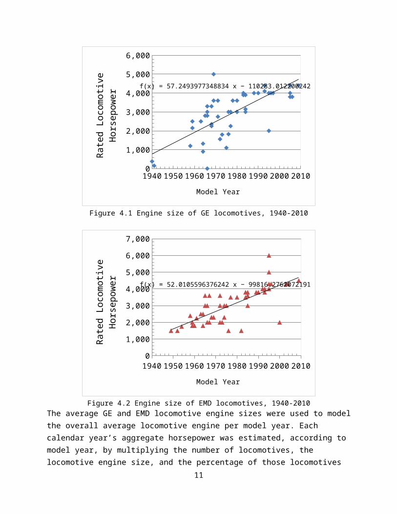
As a locomotive increases in horsepower, it can perform more work. For example, a 4,000-hp locomotive (standard in 2015) is capable of twice the work of a 2,000-hp locomotive (standard in the 1950s and 1960s). A locomotive that does twice the work will consume significantly more fuel, even when accounting for efficiency improvements over time. Thus, the fleet’s aggregate horsepower by model year provides a more accurate representation of the locomotive fleet activity than simply considering the population. plots actual GE locomotive engine size data, including the equation used to estimate the average engine size of its locomotives according to model year. Figure 4.2 plots actual EMD locomotive 5 Tier data can more accurately determine emissions than manufacture or remanufacture year, as the original locomotive manufacture year and the remanufacture year are not reliable indicators of engine Tier or emission standard due to flexibility provisions in the engine standards.6 http://en.wikipedia.org/wiki/List_of_GE_locomotives7 http://en.wikipedia.org/wiki/List_of_GM-EMD_locomotives

7

engine size data, along with the trend line equation to estimate their average engine size locomotive. The figures show how engine size has grown over time.

1940 1950 1960 1970 1980 1990 2000 20100

1,000

2,000

3,000

4,000

5,000

6,000

f(x) = 57.2493977348834 x − 110283.012200242

Model Year

Rate

d Lo

com

otive

Hor

sepo

wer

Figure 4.1 Engine size of GE locomotives, 1940-2010

1940 1950 1960 1970 1980 1990 2000 20100

1,000

2,000

3,000

4,000

5,000

6,000

7,000

f(x) = 52.0105596376242 x − 99816.2762072191

Model Year

Rate

d Lo

com

otive

Hor

sepo

wer

Figure 4.2 Engine size of EMD locomotives, 1940-2010The average GE and EMD locomotive engine sizes were used to model the overall average locomotive engine per model year. Each calendar year’s aggregate horsepower was estimated, according to model year, by multiplying the number of locomotives, the locomotive engine size,

8

and the percentage of those locomotives expected to be in service. Next, the estimated horsepower was summed across all model years to calculate each calendar year’s aggregate horsepower.

This analysis is based on historical increases in horsepower, and will be an area requiring additional study in the future to determine if locomotives continue this observed trend, or if their maximum horsepower plateaus.

4.3. Activity

The activity data is confidential because the 2007 submitted data served as a significant source for estimating activity on smaller subdivisions, and the 2011 activity data submitted was used to estimate activity on unreported-but-adjacent subdivisions. With the fuel burn estimated for each subdivision, the sum of these estimates would represent the total fuel burned by Class I locomotives during line-haul activity within California.

The model uses fuel consumption to measure locomotive activity. To determine baseline fuel use, Equation 4.1 modeled emissions from 2011 locomotive activity, with explanations for the three inputs explained in the following sections.

Equation 4.1

Emissions= (Locomotive Activity )∗( Fuel BurnedUnit of Locomotive Activity )∗( Emission factor

Unit of Fuel Burned )

4.3.1. Methodology 1: Activity by Reported Locomotive Duty Cycle

The rail companies reported the number of locomotives, by engine tier, and the corresponding duty cycles that represent each locomotive’s operations. Table 4-3 lists the subdivisions with activity data that used methodology 1.

Table 4-3 Subdivisions using Methodology 1

9

SubdivisionFresno

Los Angeles (Redondo-Riverside)Los Angeles (Cajon)

MartinezMojave

RosevilleValleyYumaCajon

San Bernardino

For these subdivisions, the process of calculating activity and fuel use by engine tier is based on reported data and U.S. EPA fuel consumption by notch, using the following steps:

1. Each subdivision is assigned a notch profile based on the rail company reports. This notch profile is a horsepower-weighted average from the rail company reports.

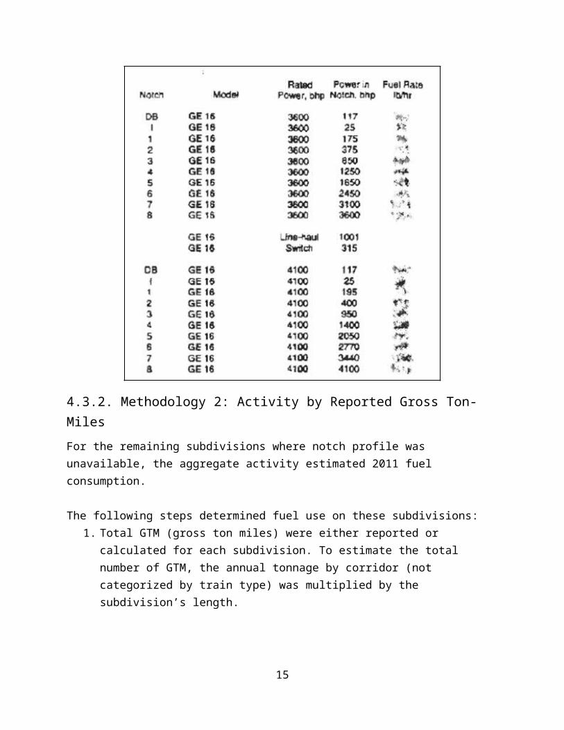
2. Each notch is assigned a fuel burn rate based on U.S. EPA test data8, shown in (with potentially confidential data blurred). The fuel burn rate is an average taken from Notch profile data for eighteen locomotive types, ranging in size from 2,500 hp to 4,100 hp.

3. The fuel burn rate by notch profile is multiplied against the weighted notch profile by subdivision, resulting in the fuel burned by subdivision.

Table 4-4 Sample throttle notch data

8 https://www3.epa.gov/otaq/documents/420r98101.pdf

10

4.3.2. Methodology 2: Activity by Reported Gross Ton-Miles

For the remaining subdivisions where notch profile was unavailable, the aggregate activity estimated 2011 fuel consumption.

The following steps determined fuel use on these subdivisions:1. Total GTM (gross ton miles) were either reported or calculated for each subdivision. To

estimate the total number of GTM, the annual tonnage by corridor (not categorized by train type) was multiplied by the subdivision’s length.

2. Rail productivity (measured in GTM/gallon of fuel) was estimated to determine the amount of fuel required to move the tonnage over the track’s distance.

3. The activity rate (measured in GTM/hour per locomotive) was divided by the fuel burn rate (measured in gal/hr per locomotive) to estimate the fuel productivity for each train type on each subdivision.

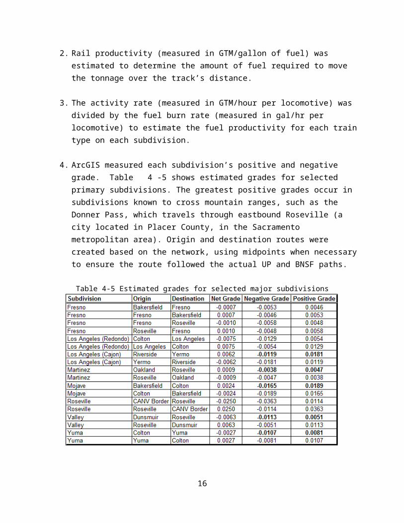
4. ArcGIS measured each subdivision’s positive and negative grade. Table 4-5 shows estimated grades for selected primary subdivisions. The greatest positive grades occur in

11

subdivisions known to cross mountain ranges, such as the Donner Pass, which travels through eastbound Roseville (a city located in Placer County, in the Sacramento metropolitan area). Origin and destination routes were created based on the network, using midpoints when necessary to ensure the route followed the actual UP and BNSF paths.

Table 4-5 Estimated grades for selected major subdivisions

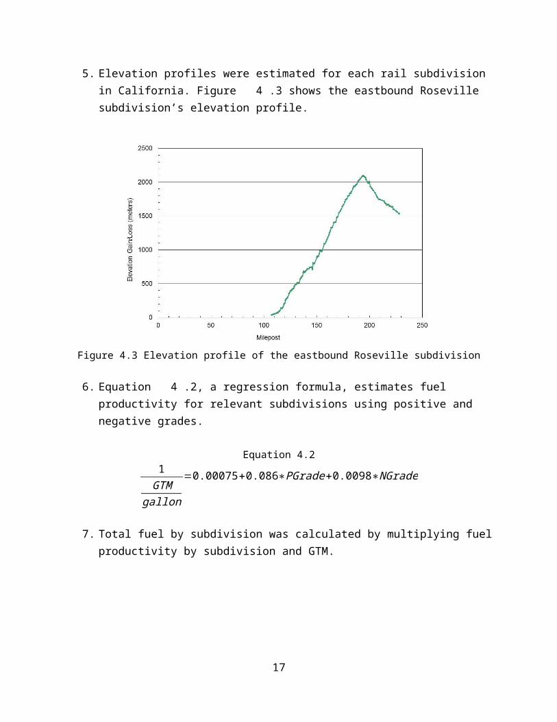
5. Elevation profiles were estimated for each rail subdivision in California. Figure 4.3 shows the eastbound Roseville subdivision’s elevation profile.

12

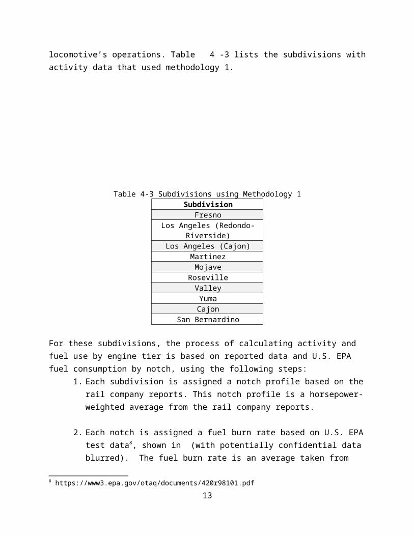
Figure 4.3 Elevation profile of the eastbound Roseville subdivision

6. Equation 4.2, a regression formula, estimates fuel productivity for relevant subdivisions using positive and negative grades.

Equation 4.21

GTMgallon

=0.00075+0.086∗PGrade+0.0098∗NGrade

7. Total fuel by subdivision was calculated by multiplying fuel productivity by subdivision and GTM.

4.3.3. Methodology 3: Activity by Estimated Locomotive-Hours

The remaining networks could not use the first two methodologies, whose subdivisions are shown in Table 4-6. Activity was estimated using the number of locomotives operating on the subdivision, the average time spent by each locomotive passing through the subdivision, and the amount of fuel burned by each locomotive during each unit of time.

Table 4-6 Remaining subdivision activity estimated using external sources

13

SubdivisionAlameda Corridor

HarborLucerne

OliveRiverbankSan DiegoSan JacintoSeligman

Black ButteCanyonFresnoMojave

PalmdaleRoseville

Sac1/2Valley

The following steps were taken to account for fuel in these subdivisions:1. Public data sources were used to estimate the number of locomotives. For example,

Alameda Corridor data was retrieved from the Alameda Corridor Transportation Authority9. Equation 4.3 calculates average time spent by each locomotive passing through a subdivision, and required data from other subdivisions to estimate the average speed of locomotives. Then, it was divided by the length of each subdivision.

Equation 4.3Average Speed (mph)=22.8−136.2∗PGrade−42.5∗NGrade

Because activity data was not reported for these subdivisions, activity could not be classified by train type (Premium, Manifest/Bulk, or Other), which can make a difference since Premium trains travel faster than the others. Using Equation 4.3, the average speed appeared to be highest on flat segments, decreasing for both uphill and downhill segments. To estimate the average time spent by each locomotive on each subdivision, the locomotive’s average speed was divided by the distance.

2. To estimate the fuel burned during each locomotive hour, a method similar to Methodology 2 was used. Equation 4.4 shows the fuel burn rate (measured in gal/hr) regression as a function of the grade for each subdivision, where NGrade has a negative value, allowing the fuel burn rate to decrease as the grade becomes more negative. Grades were measured in the same manner as with Methodology 2, when modeling fuel productivity (GTM/gallon) as a function of grade.

9 http://www.acta.org/

14

Equation 4.4

Fuel Burn Rate ( gallonshour )=44.4+1949∗PGrade+407∗NGrade

4.4. Growth

The model growth assumptions are a compilation of two factors: growth of the industry (measured by the total amount of freight ton-miles) and improvements in fuel efficiency. These two factors work in opposition because increased freight totals require more fuel while improved efficiency allows the rail operations to spend less fuel per freight-ton-mile.

The 2015 Freight Analysis Framework10 (FAF) projections for rail within California predict rail freight growth. The growth from 2015 to 2040 increases approximately 54%, corresponding to approximately 2.1% annually.

shows rail growth factors across the state, as well as regionally.

Table 4-7 FAF Rail Growth Rates by Area of CaliforniaLos

AngelesSan

Francisco San Diego Sacramento Rest of California State Total

2.12% 2.08% 1.78% 2.33% 2.07% 2.10%

In a future model, growth may be split by region. However, the statewide growth was applied to the entire rail inventory. Ultimately, this has little statistical significance on the outcome, as the growth rates in localized areas varied from the statewide growth by a small fraction of a percent.

Figure 4.4 shows activity growth based on the updated analysis, compared to the previous activity, as well as the Freight Analysis Framework (FAF) data, relative to 2011 activity.

10 Freight Analysis Framework. https://www.rita.dot.gov/bts/sites/rita.dot.gov.bts/files/subject_areas/freight_transportation/faf

15

2000 2005 2010 2015 2020 2025 2030 2035 2040 2045 20500.0

0.5

1.0

1.5

2.0

2.5

3.0

3.5

4.0

4.5

5.02015 FAF LA Total2015 FAF CA Total RatePrevious Rail Activity GrowthUpdated Rail Activity

Grow

th R

elati

ve to

201

1/20

12 B

asel

ine

Figure 4.4 Locomotive Activity Growth

The increase in fuel efficiency results from discussions with UP and BNSF, who predict the industry will average approximately 1% increases annually in fuel efficiency. This increase is based on the industry’s historical averages, as well as projections of upcoming technological improvements.

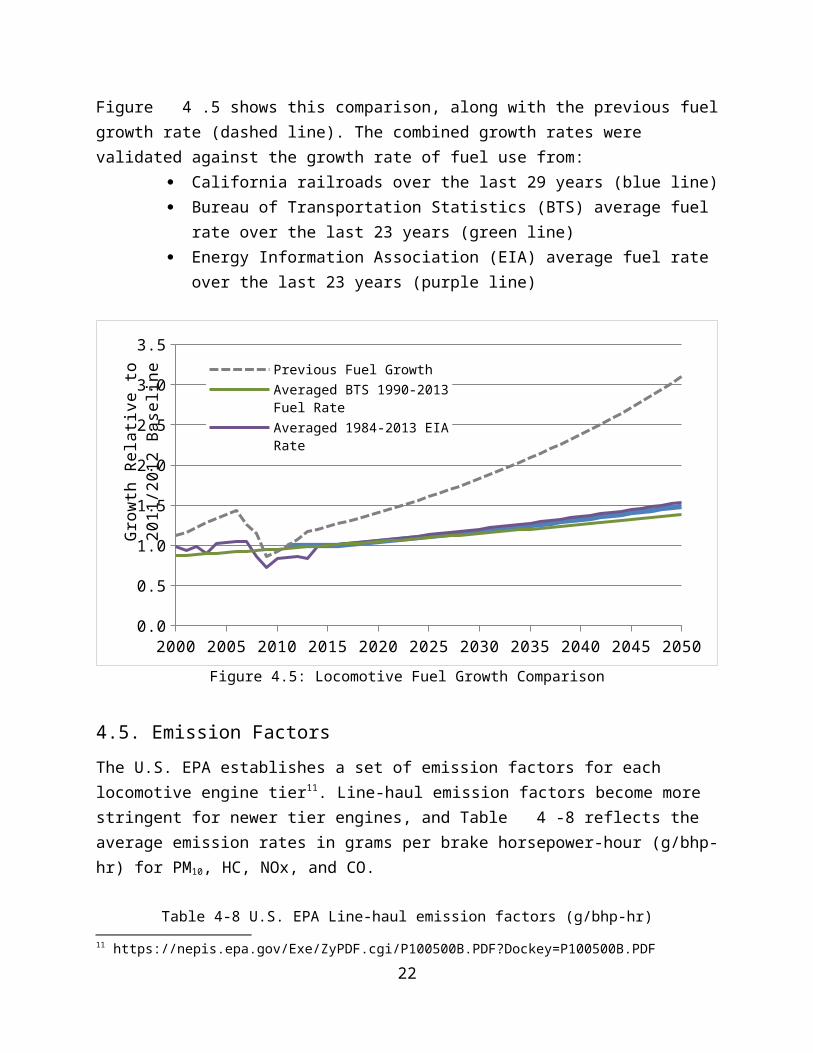
Figure 4.5 shows this comparison, along with the previous fuel growth rate (dashed line). The combined growth rates were validated against the growth rate of fuel use from:

California railroads over the last 29 years (blue line) Bureau of Transportation Statistics (BTS) average fuel rate over the last 23 years

(green line) Energy Information Association (EIA) average fuel rate over the last 23 years

(purple line)

16

2000 2005 2010 2015 2020 2025 2030 2035 2040 2045 20500.0

0.5

1.0

1.5

2.0

2.5

3.0

3.5

Previous Fuel GrowthAveraged BTS 1990-2013 Fuel RateAveraged 1984-2013 EIA RateUpdated Rail Fuel

Grow

th R

elati

ve to

201

1/20

12 B

asel

ine

Figure 4.5: Locomotive Fuel Growth Comparison

4.5. Emission Factors

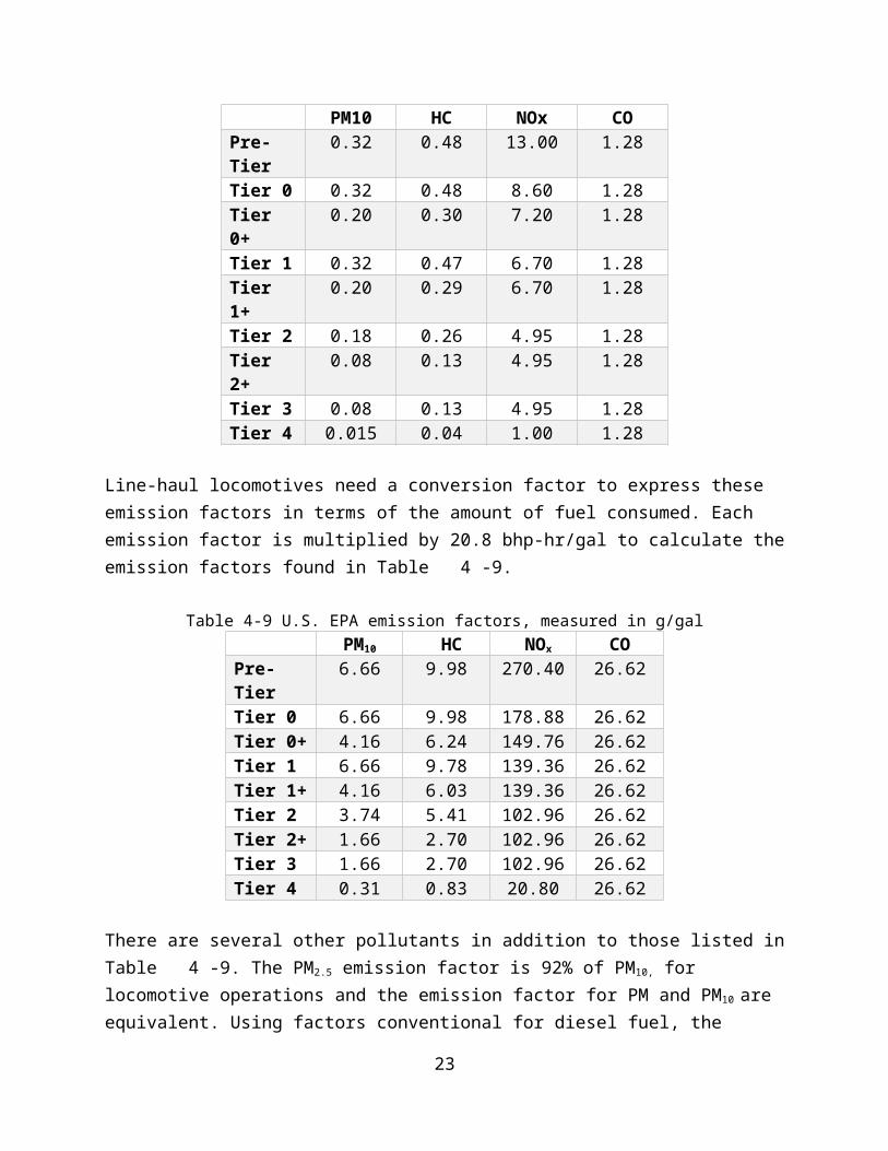
The U.S. EPA establishes a set of emission factors for each locomotive engine tier11. Line-haul emission factors become more stringent for newer tier engines, and Table 4-8 reflects the average emission rates in grams per brake horsepower-hour (g/bhp-hr) for PM10, HC, NOx, and CO.

Table 4-8 U.S. EPA Line-haul emission factors (g/bhp-hr)PM10 HC NOx CO

Pre-Tier 0.32 0.48 13.00 1.28Tier 0 0.32 0.48 8.60 1.28Tier 0+ 0.20 0.30 7.20 1.28Tier 1 0.32 0.47 6.70 1.28Tier 1+ 0.20 0.29 6.70 1.28Tier 2 0.18 0.26 4.95 1.28Tier 2+ 0.08 0.13 4.95 1.28Tier 3 0.08 0.13 4.95 1.28Tier 4 0.015 0.04 1.00 1.28

Line-haul locomotives need a conversion factor to express these emission factors in terms of the amount of fuel consumed. Each emission factor is multiplied by 20.8 bhp-hr/gal to calculate the emission factors found in Table 4-9.

11 https://nepis.epa.gov/Exe/ZyPDF.cgi/P100500B.PDF?Dockey=P100500B.PDF

17

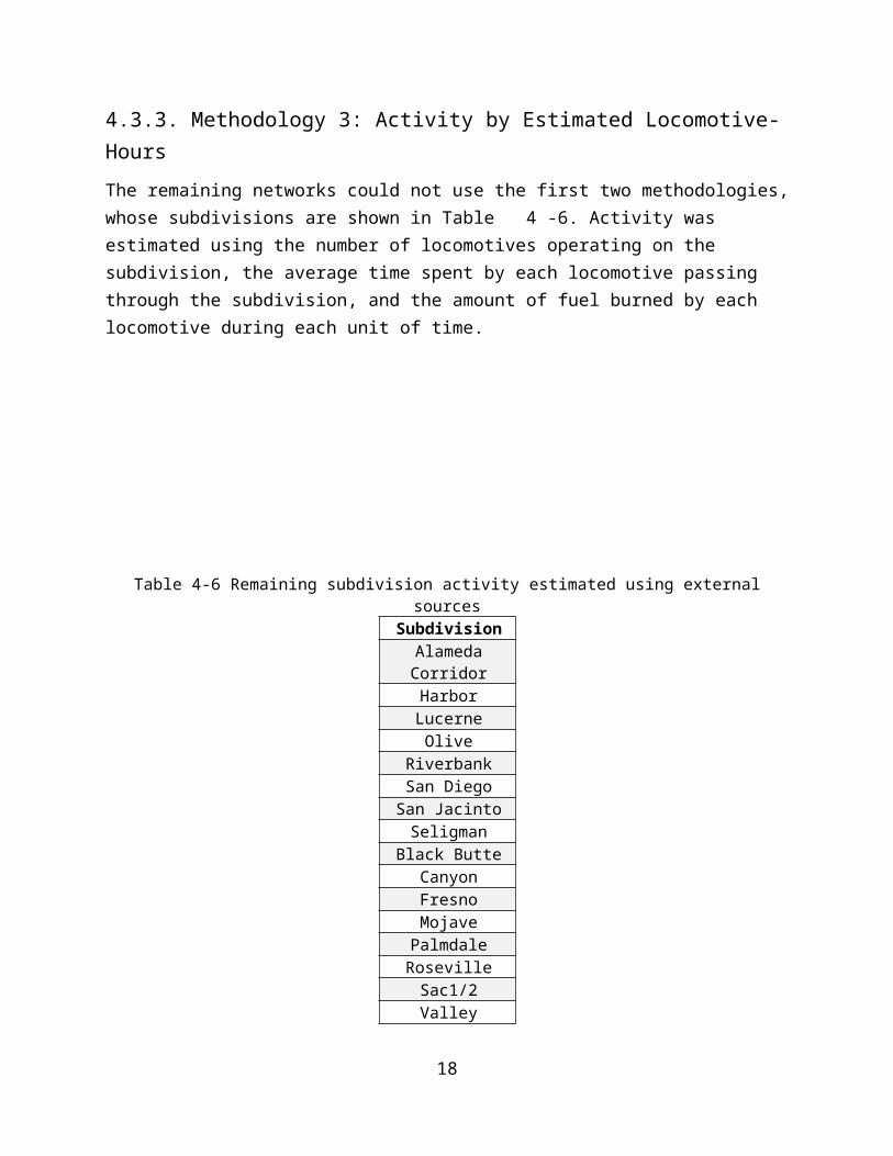
Table 4-9 U.S. EPA emission factors, measured in g/gal  PM10 HC NOx COPre-Tier 6.66 9.98 270.40 26.62Tier 0 6.66 9.98 178.88 26.62Tier 0+ 4.16 6.24 149.76 26.62Tier 1 6.66 9.78 139.36 26.62Tier 1+ 4.16 6.03 139.36 26.62Tier 2 3.74 5.41 102.96 26.62Tier 2+ 1.66 2.70 102.96 26.62Tier 3 1.66 2.70 102.96 26.62Tier 4 0.31 0.83 20.80 26.62

There are several other pollutants in addition to those listed in Table 4-9. The PM2.5 emission factor is 92% of PM10, for locomotive operations and the emission factor for PM and PM10 are equivalent. Using factors conventional for diesel fuel, the emission factor for total organic gases is estimated as 1.44 times the emission factor for hydrocarbons (HC), and the emission factor for reactive organic gases is estimated as 1.21 times the emission factor for hydrocarbons (HC). The emission factor for NH3 is estimated as 0.0833 g/gal of fuel, independent of tier. CO2 is defined by U.S. EPA as 10,206 g CO2/gal of fuel.

4.5.1. Emission Adjustments

When locomotives refuel within California, they receive CARB (California Air Resources Board) diesel. CARB diesel is an ultra-low sulfur diesel fuel, and therefore reduces NOx emissions by 6% and PM by 14%12. ARB regulation passed in 2004 requires intrastate locomotives (those with more than 90% of fuel consumption occurring in California) use CARB diesel.The U.S. EPA uses Equation 4.5 to calculate SO2 emission factors13.

Equation 4.5SO2=[ BSFC∗453.6∗(1−SOx cnv )−HC ]∗SOxdsl∗2

where SO2 is in g/hp-hr BSFC is the in-use adjusted fuel consumption in lb/hp-hr 453.6 is the conversion factor from pounds to grams SOxcnv is the fraction of fuel sulfur converted to direct PM HC is the in-use adjusted hydrocarbon emissions in g/hp-hr SOxdsl is the episodic weight percent of sulfur in nonroad diesel fuel2 is the grams of SO2 formed from a gram of sulfur

12 https://www.arb.ca.gov/railyard/diesel/cadieselfuelreg.htm13 EQ7 from https://www3.epa.gov/otaq/models/nonrdmdl/nonrdmdl2010/420r10018.pdf

18

Emissions estimates for line-haul locomotive activity in California consisted of five steps:1. Estimate annual fuel consumption for each corridor.

2. Allocate the fuel modeled for each corridor to the corresponding geographic area of

interest.

3. Model the tier distribution associated with each corridor or geographic area of interest.

4. Calculate the emissions based on the fuel consumption and tier distribution.

4.6. Spatial and Temporal Allocation

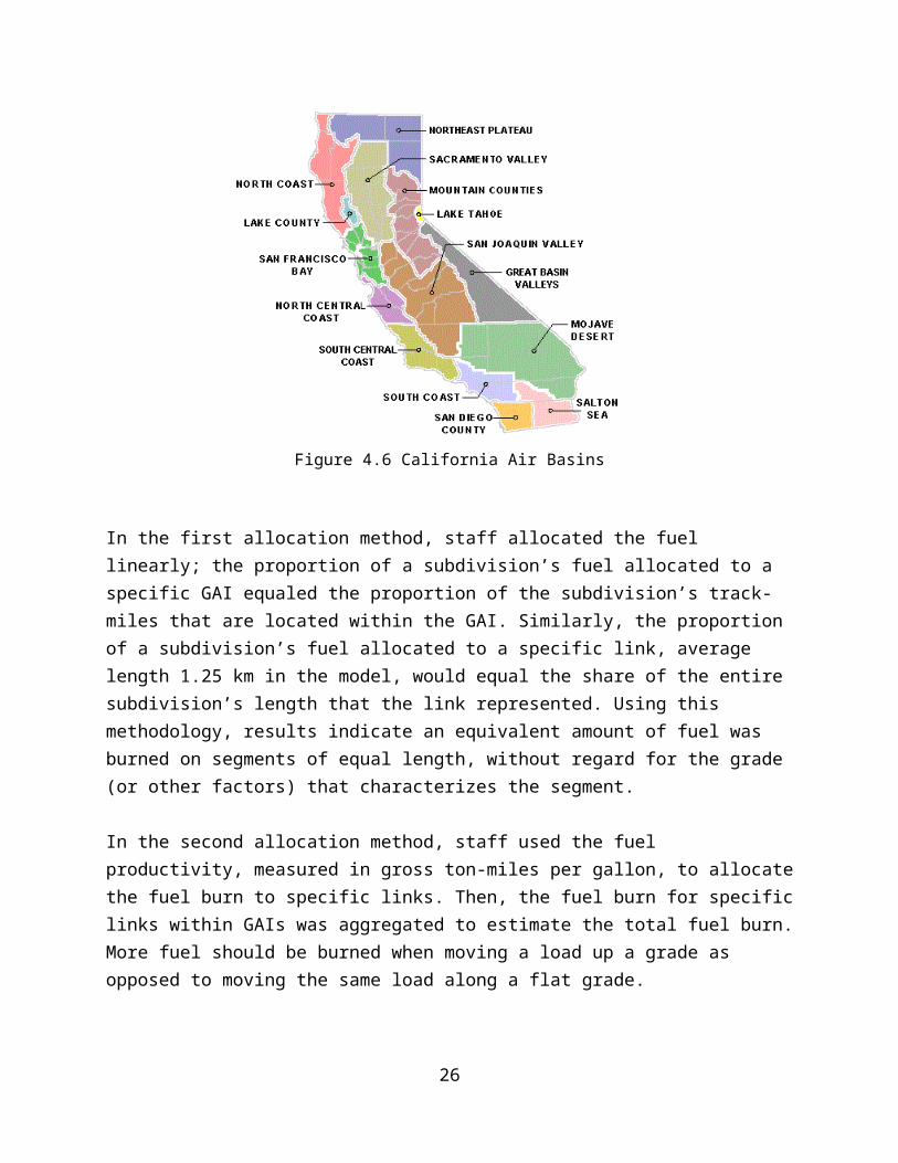
Each subdivision’s fuel estimates were aggregated, using the methodology in the preceding section. Then, fuel was geographically allocated to the GAIs (Geographical Area of Interest) for calendar year 2011, according to air basin, district, and county. Each air basin is comprised of multiple counties and air districts, and some counties are divided between air basins or air districts14, depicted by the map in Figure 4.6. California is divided into 15 Air Basins, 35 Air Districts, and 58 counties. Activity proportions were allocated in two different ways.

Figure 4.6 California Air Basins

In the first allocation method, staff allocated the fuel linearly; the proportion of a subdivision’s fuel allocated to a specific GAI equaled the proportion of the subdivision’s track-miles that are located within the GAI. Similarly, the proportion of a subdivision’s fuel allocated to a specific link, average length 1.25 km in the model, would equal the share of the entire subdivision’s

14 http://www.arb.ca.gov/ei/maps/statemap/abmap.htm

19

length that the link represented. Using this methodology, results indicate an equivalent amount of fuel was burned on segments of equal length, without regard for the grade (or other factors) that characterizes the segment.

In the second allocation method, staff used the fuel productivity, measured in gross ton-miles per gallon, to allocate the fuel burn to specific links. Then, the fuel burn for specific links within GAIs was aggregated to estimate the total fuel burn. More fuel should be burned when moving a load up a grade as opposed to moving the same load along a flat grade.

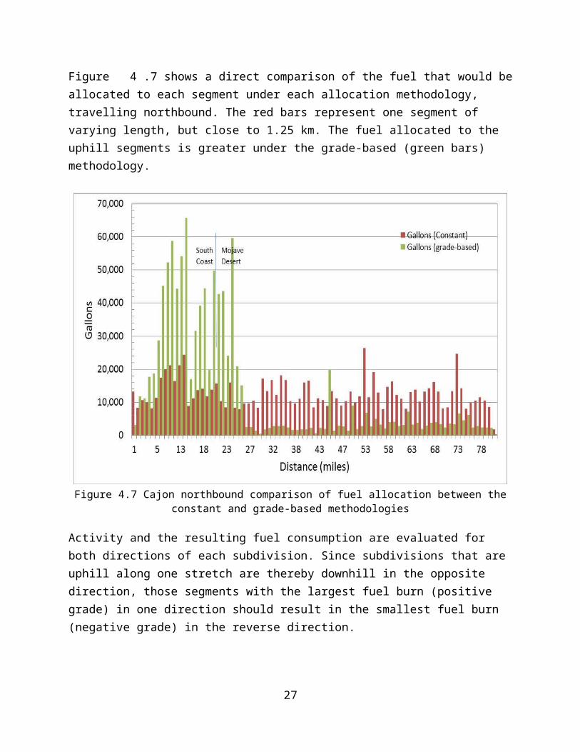
Figure 4.7 shows a direct comparison of the fuel that would be allocated to each segment under each allocation methodology, travelling northbound. The red bars represent one segment of varying length, but close to 1.25 km. The fuel allocated to the uphill segments is greater under the grade-based (green bars) methodology.

Figure 4.7 Cajon northbound comparison of fuel allocation between the constant and grade-based methodologies

Activity and the resulting fuel consumption are evaluated for both directions of each subdivision. Since subdivisions that are uphill along one stretch are thereby downhill in the opposite direction, those segments with the largest fuel burn (positive grade) in one direction should result in the smallest fuel burn (negative grade) in the reverse direction.

20

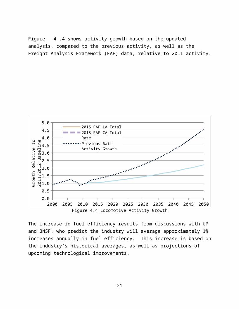
Figure 4.8 shows a comparison from each method’s allocation for southbound moving trains. The grade-based (green bar) fuel burn is largely removed from the South Coast Air Basin (which is downhill southbound), and instead allocates fuel to the segments found in the Mojave Desert Air Basin.

Figure 4.8 Cajon southbound comparison of fuel allocation between the constant and grade-based methodologies

Table 4-10 shows allocation differences when aggregated across a Cajon subdivision segment. The segment length is defined by the activity reported, which are the locations where crew may be switched or measurements recorded. These locations may not correspond to the designated start and finish of the Cajon subdivision.

Table 4-10 Comparison of constant and grade-based allocation

21

Direction Air basin Constant Grade-based AverageSouth Coast 24% 56% 40%Mojave Desert 76% 44% 60%South Coast 24% 3% 14%Mojave Desert 76% 97% 86%

Northbound

Southbound

Fuel burn rates increase with each notch. One concern with the grade-based fuel methodology is the frequency with which train operators shift from one notch to another. Train operators are more likely to shift notches for an extended change in grade instead of a small hill, particularly since the train length can exceed the distance of shorter hills. Because of this uncertainty, and the recognition that GIS can only imperfectly reflect rail links, staff used the average fuel burn that would be estimated under the two methodologies. Table 4-11 lists 2011 estimated fuel burn for select air basins.

Table 4-11 The 2011 estimated fuel burn for select California air basinsAir Basin Fuel

MC 12,063,150 MD 89,873,601 NCC 226,306 NEP 7,390,256 SC 37,468,647

SCC 763,036 SD 2,422,878 SF 5,218,136

SJV 25,299,243 SS 17,722,463 SV 11,548,300

5. TURNOVER AND RULE ANALYSIS

The locomotive survival curve is a forecasting method that estimates the useful life of a locomotive. The survival curve depicts the number of locomotives still in operation as they age, and is used to model future year population distributions.

5.1. Baseline Natural Turnover

The survival curve applied to locomotives was developed using the combined 2011 UP and BNSF Tier data. The tier distribution and remanufactured tier distribution data was correlated with specific model years, developing a model-year specific base population. Remanufactured engine data was collected from an EPA locomotive emissions report (Control of Emissions of Air Pollution from Locomotive Engines and Marine Compression-Ignition Engines Less Than 30

22

Liters per Cylinder15). Adding the original locomotive engines and the remanufactured locomotive engine distributions together created the locomotive survival/lifecycle curve in Figure 5.9.

0 5 10 15 20 25 30 35 40 450%

20%

40%

60%

80%

100%

120%

Age (years)

Surv

ival

Rat

e

Figure 5.9 Locomotive Survival Curve / Life-cycle

Based on conversations with locomotive manufacturers, ARB estimated the typical line-haul locomotive will be remanufactured twice, about once every 7 years, and remains in service slightly more than 21 years in total. There is a spike in Figure 5.9 due to the first incidence of remanufactured locomotives. There is a dramatic decrease in the locomotive survival rate around 15 years of age; a majority of these engines are near the end of their life and begin to be removed from long distance (interstate) line-haul service, being placed in regional service until they are no longer used as line haul locomotives. At this point, after about 21 years, they may be used as switchers (no longer represented on the survival curve) or be retired.

5.2. Fleet Sales

To project future sales, staff created a best-fit polynomial to project the locomotive sales for the state of California, and used the overall growth rate projected for locomotive fuel (described previously in Section 3.3 on page 15). This method has the underlying assumption that locomotives in future years will generally see the same annual activity, expressed in terms of fuel used, as did the UP and BNSF locomotives in the 2011 and 2014 reports. This keeps the growth of locomotive sales (new locomotives entering the fleet) at the same rate as the growth of overall

15 https://www.gpo.gov/fdsys/pkg/FR-2008-06-30/pdf/R8-7999.pdf

23

locomotive fuel use. Figure 5.10 shows the estimated previous sales of locomotives, the actual 2004-2012 locomotive sales taken from data reported to ARB, and the forecasted locomotive sales.

Figure 5.10 Projected and Back-Casted Locomotive Sales

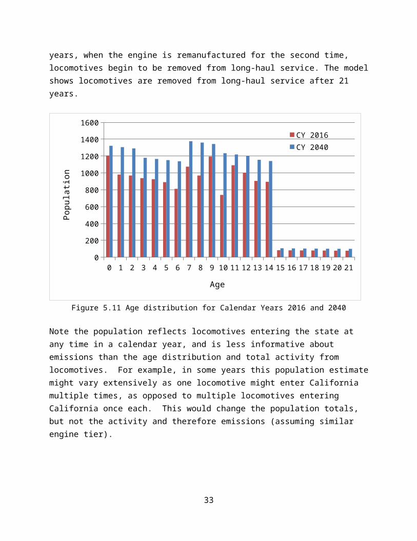
Figure 5.11 shows the locomotive age distribution in calendar years 2016 and 2040 resulting from combining the survival curve and sales. There is a slight population increase when locomotives reach about 7 years of age, due to remanufacturing. After 15 years, when the engine is remanufactured for the second time, locomotives begin to be removed from long-haul service. The model shows locomotives are removed from long-haul service after 21 years.

24

0 1 2 3 4 5 6 7 8 9 10 11 12 13 14 15 16 17 18 19 20 210

200

400

600

800

1000

1200

1400

1600

CY 2016CY 2040

Age

Popu

latio

n

Figure 5.11 Age distribution for Calendar Years 2016 and 2040

Note the population reflects locomotives entering the state at any time in a calendar year, and is less informative about emissions than the age distribution and total activity from locomotives. For example, in some years this population estimate might vary extensively as one locomotive might enter California multiple times, as opposed to multiple locomotives entering California once each. This would change the population totals, but not the activity and therefore emissions (assuming similar engine tier).

6. EMISSION RESULTS

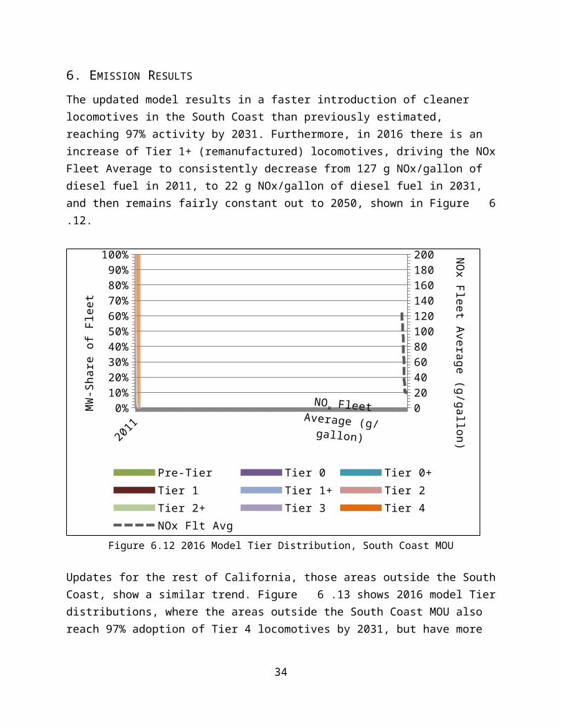
The updated model results in a faster introduction of cleaner locomotives in the South Coast than previously estimated, reaching 97% activity by 2031. Furthermore, in 2016 there is an increase of Tier 1+ (remanufactured) locomotives, driving the NOx Fleet Average to consistently decrease from 127 g NOx/gallon of diesel fuel in 2011, to 22 g NOx/gallon of diesel fuel in 2031, and then remains fairly constant out to 2050, shown in Figure 6.12.

25

20110%

10%

20%

30%

40%

50%

60%

70%

80%

90%

100%

0

20

40

60

80

100

120

140

160

180

200

Pre-Tier Tier 0 Tier 0+Tier 1 Tier 1+ Tier 2Tier 2+ Tier 3 Tier 4NOx Flt Avg

MW

-Sha

re o

f Fle

etNO

x Fleet Average (g/gallon)

NOx Fleet Average (g/gallon)

Figure 6.12 2016 Model Tier Distribution, South Coast MOU

Updates for the rest of California, those areas outside the South Coast, show a similar trend. Figure 6.13 shows 2016 model Tier distributions, where the areas outside the South Coast MOU also reach 97% adoption of Tier 4 locomotives by 2031, but have more remanufactured Tier 1 and less Tier 2 locomotives than the South Coast. This difference is due to the 1998 South Coast MOU.

26

20110%

10%

20%

30%

40%

50%

60%

70%

80%

90%

100%

0

20

40

60

80

100

120

140

160

180

200

Pre-Tier Tier 0 Tier 0+Tier 1 Tier 1+ Tier 2Tier 2+ Tier 3 Tier 4NOx Flt Avg

MW

-Sha

re o

f Fle

etNO

x Fleet Average (g/gallon)

NOx Fleet Average (g/gallon)

Figure 6.13 2016 Model Tier Distribution, outside the South Coast

Figure 6.14 and Figure 6.15 show the resulting emissions for NOx and PM for the South Coast, and in Figure 6.16 and Figure 6.17 for California statewide emissions. The figures show NOx and PM emissions have an inverse relationship during 2000 to 2005. NOx emissions decline due to NOx emission factor reductions (see Table 4-8). PM emission factors remain constant. Combining the emission factor information with expected growth rates result in PM emissions growth from 2000 to 2005. In 2005, with the introduction of Tier 2 standards, there is a dramatic reduction in PM emission factors, and further reductions in NOx emission factors. Hence, both NOx and PM show large reductions beginning in 2005, and estimated to continue reducing emissions in the future.

27

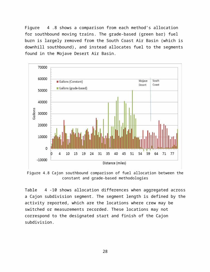
Figure 6.14 South Coast NOx

Figure 6.15 South Coast PM

28

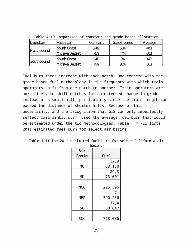
Figure 6.16 California statewide NOx

Figure 6.17 California statewide PM

Table 6-12 provides an overview of select years for NOx, PM, and fuel usage for the South Coast and California. The entire list of yearly emissions is located in Table 8-13.

29

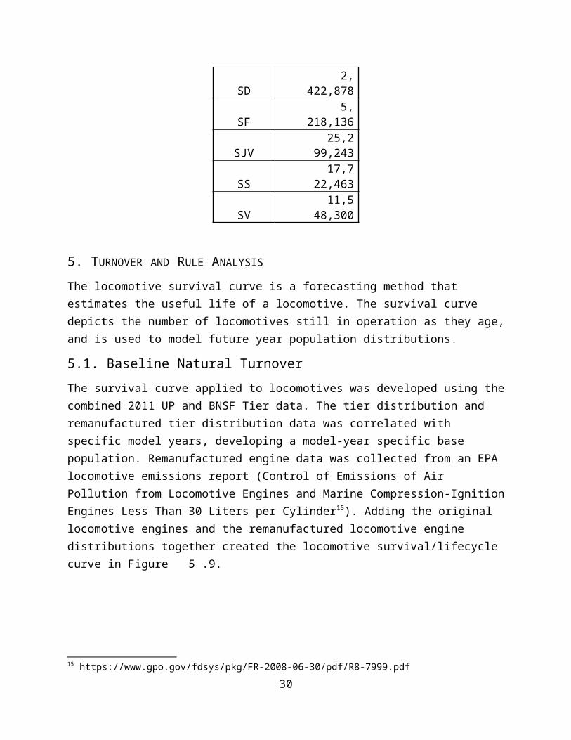
Table 6-12 NOx, PM, and Fuel for Selected Year  NOx (tpd) PM (tpd) Fuel (gal/year)  South Coast California South Coast California South Coast California

2010 13.18 78.15 0.35 2.13 35,071,697 197,219,5752017 11.40 63.91 0.20 1.13 37,891,076 212,363,5542023 7.82 43.84 0.12 0.65 40,649,338 227,822,4552031 3.08 17.27 0.04 0.25 44,641,852 250,198,817

7. VALIDATION AND QUALITY ASSURANCE

The 2016 locomotive model update used updated assumptions and some new data. The largest changes resulted from updating the growth rate based on FAF 2015, and model year distribution forecasts based on actual 2011 and 2014 UP and BNSF data. The 2011 and 2014 rail data were used to check the validity of the updated locomotive model. As evident in Figure 7.18 and Figure7.19, combining the Tier 0 original manufacture with the Tier 0+ remanufactured locomotives, and doing the same for Tier 1 with Tier 1+ (and Tier 2 with Tier 2+ for 2014), demonstrate the model produces results that are comparable to the actual rail reported data. However, there is limited data explaining how to properly link the original manufacture year and the remanufactured year to the appropriate Tier level. Tier data reports accurate emissions data, but does not necessarily correlate to locomotive model years, causing difficulty when creating projections.

Figure 7.18 2011 South Coast and rest of California Tier comparisons

30

Figure 7.19 2014 South Coast and rest of California Tier comparisons

8. SOUTH COAST AND STATEWIDE EMISSIONS RESULTS

Table 8-13 summarizes NOx and PM criteria emissions and fuel consumption for line-haul locomotives operating in California, based on the 2016 Line-Haul Locomotive model. Results shown are for the South Coast Air Basin and the entire state of California.

Table 8-13 Emissions Results for South Coast and statewideNOx (tpd) PM (tpd) Fuel (gal/year)

South Coast

California South Coast

California South Coast California

1990

25.02 143.04 0.59 3.38 31,589,532 180,579,048

1991

25.53 145.49 0.60 3.44 32,224,064 183,677,279

1992

26.04 148.02 0.62 3.50 32,878,297 186,871,345

1993

26.58 150.63 0.63 3.56 33,552,849 190,164,245

1994

27.13 153.32 0.64 3.62 34,248,355 193,559,071

1995

27.70 156.09 0.65 3.69 34,965,469 197,059,013

1996

28.61 160.84 0.68 3.80 36,118,459 203,052,795

199 30.03 168.42 0.71 3.98 37,913,555 212,620,300

31

7199

830.79 172.26 0.73 4.07 38,872,372 217,465,146

1999

31.99 178.56 0.76 4.22 40,391,468 225,416,085

2000

30.47 169.64 0.77 4.28 41,129,555 228,983,631

2001

29.20 161.89 0.79 4.36 42,014,966 232,911,947

2002

28.13 155.31 0.81 4.50 43,563,264 240,496,604

2003

27.61 152.52 0.86 4.73 45,828,684 253,130,086

2004

26.88 148.54 0.89 4.93 47,718,315 263,715,575

2005

25.88 143.11 0.90 4.96 49,791,976 275,345,336

2006

25.13 137.97 0.88 4.95 51,190,134 283,034,562

2007

21.56 118.52 0.58 3.38 46,641,245 260,871,676

2008

18.21 101.82 0.49 2.87 42,008,444 234,088,946

2009

13.45 77.94 0.36 2.16 33,239,945 187,533,680

2010

13.18 78.15 0.35 2.13 35,071,697 197,219,575

2011

13.55 79.93 0.35 2.14 37,468,647 209,996,015

2012

13.02 76.71 0.29 1.82 37,464,900 209,975,015

2013

12.56 73.90 0.26 1.65 37,461,153 209,954,018

2014

12.15 71.39 0.24 1.49 37,457,407 209,933,022

2015

11.82 69.33 0.21 1.36 37,453,661 209,912,029

2016

11.36 66.67 0.19 1.23 37,449,916 209,891,038

2017

11.40 63.91 0.20 1.13 37,891,076 212,363,554

2018

10.64 59.66 0.18 0.99 38,337,433 214,865,197

2019

9.87 55.29 0.15 0.84 38,789,048 217,396,309

2020

9.34 52.34 0.14 0.77 39,245,983 219,957,238

32

2021

8.86 49.65 0.13 0.74 39,708,301 222,548,334

2022

8.32 46.63 0.12 0.69 40,176,064 225,169,953

2023

7.82 43.84 0.12 0.65 40,649,338 227,822,455

2024

7.18 40.25 0.11 0.60 41,128,188 230,506,204

2025

6.57 36.80 0.10 0.55 41,612,678 233,221,567

2026

5.92 33.19 0.09 0.50 42,102,875 235,968,917

2027

5.33 29.89 0.08 0.44 42,598,847 238,748,631

2028

4.75 26.63 0.07 0.39 43,100,661 241,561,090

2029

4.18 23.42 0.06 0.34 43,608,387 244,406,679

2030

3.63 20.36 0.05 0.30 44,122,094 247,285,790

2031

3.08 17.27 0.04 0.25 44,641,852 250,198,817

2032

3.06 17.18 0.04 0.25 45,167,733 253,146,159

2033

3.05 17.07 0.04 0.25 45,699,809 256,128,220

2034

3.02 16.95 0.04 0.24 46,238,153 259,145,411

2035

3.00 16.84 0.04 0.24 46,782,838 262,198,144

2036

2.99 16.74 0.04 0.24 47,333,940 265,286,838

2037

2.97 16.64 0.04 0.24 47,891,534 268,411,917

2038

2.95 16.55 0.04 0.24 48,455,696 271,573,809

2039

2.99 16.74 0.04 0.24 49,026,504 274,772,949

2040

3.02 16.94 0.04 0.24 49,604,036 278,009,774

2041

3.06 17.14 0.04 0.24 50,188,372 281,284,729

2042

3.09 17.34 0.04 0.25 50,779,591 284,598,263

2043

3.13 17.55 0.04 0.25 51,377,775 287,950,831

204 3.17 17.75 0.05 0.25 51,983,005 291,342,892

33

4204

53.20 17.96 0.05 0.26 52,595,365 294,774,911

2046

3.24 18.17 0.05 0.26 53,214,938 298,247,359

2047

3.28 18.39 0.05 0.26 53,841,810 301,760,713

2048

3.32 18.60 0.05 0.27 54,476,067 305,315,454

2049

3.36 18.82 0.05 0.27 55,117,795 308,912,070

2050

3.40 19.04 0.05 0.27 55,767,082 312,551,055

34