Technical Appendix for - Warringtonbear.warrington.ufl.edu/centers/MKS/appendices/Results on the... · by Adam Duhachek, Anne T. Coughlan, and Dawn Iacobucci p. 4 of 27 pp. substitutes

Technical Appendix for: “Results on the Standard Error of the Coefficient Alpha Index of Reliability”

by Adam Duhachek, Anne T. Coughlan, and Dawn Iacobucci1

April 2005

1Duhachek is a professor of marketing at Indiana University, Coughlan is a professor of marketing at Northwestern University, and Iacobucci is a professor of marketing at Wharton. The authors are grateful to Professor Steve Shugan, the AE and Reviewers, participants at the European ACR meeting, and seminar attendees from the marketing departments at the University of Colorado; University of Michigan; Northwestern University; Notre Dame and the University of Southern California for their helpful feedback on this research. Please address correspondence to the first author at: [email protected].

Technical Appendix for “Results on the Standard Error of the Coefficient Alpha Index of Reliability” by Adam Duhachek, Anne T. Coughlan, and Dawn Iacobucci

p. 1 of 27 pp.

mailto:[email protected]

Technical Appendix for: “Results on the Standard Error of the Coefficient Alpha Index of Reliability”

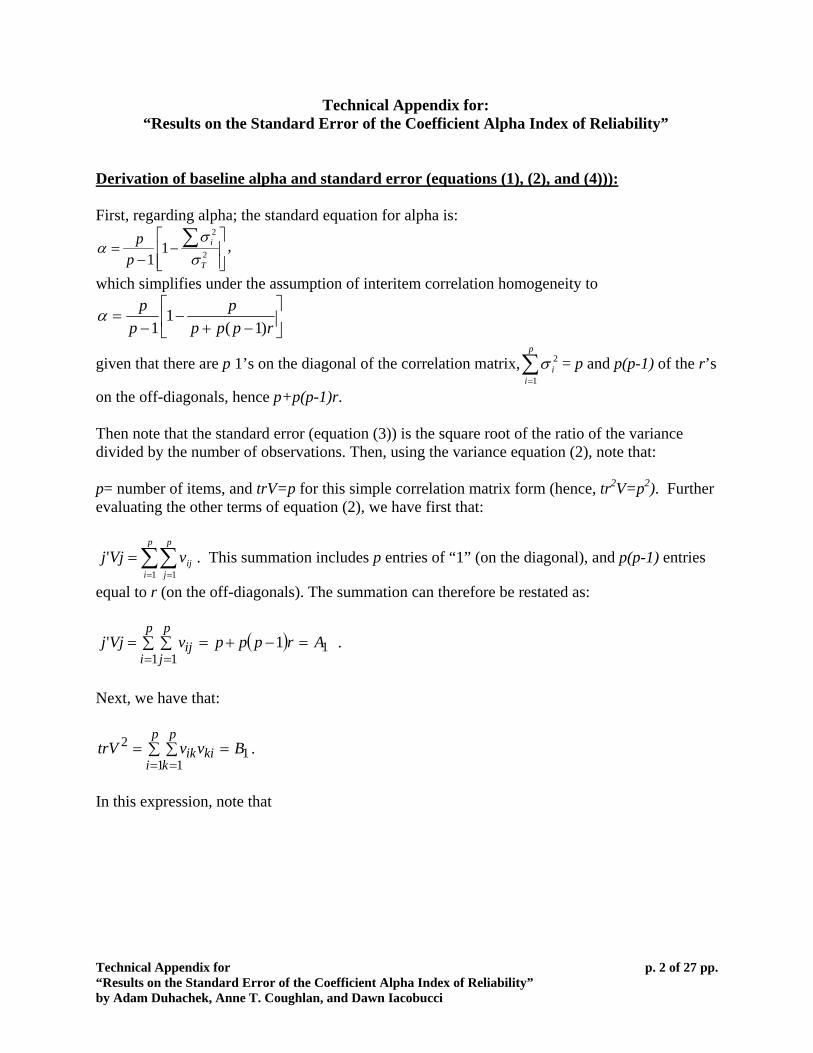
Derivation of baseline alpha and standard error (equations (1), (2), and (4))): First, regarding alpha; the standard equation for alpha is:

⎥⎥⎦

⎤

⎢⎢⎣

⎡−

−= ∑

2

2

11 T

i

pp

σσ

α ,

which simplifies under the assumption of interitem correlation homogeneity to

⎥⎦

⎤⎢⎣

⎡−+

−−

=rppp

pp

p)1(

11

α

given that there are p 1’s on the diagonal of the correlation matrix,∑ = p and p(p-1) of the r’s

on the off-diagonals, hence p+p(p-1)r. =

p

ii

1

2σ

Then note that the standard error (equation (3)) is the square root of the ratio of the variance divided by the number of observations. Then, using the variance equation (2), note that: p= number of items, and trV=p for this simple correlation matrix form (hence, tr2V=p2). Further evaluating the other terms of equation (2), we have first that:

∑∑= =

=p

i

p

jijvVjj

1 1' . This summation includes p entries of “1” (on the diagonal), and p(p-1) entries

equal to r (on the off-diagonals). The summation can therefore be restated as:

( ) 11 1

1' ArpppvVjjp

i

p

jij =−+=∑ ∑=

= = .

Next, we have that:

11 1

2 BvvtrVp

i

p

kkiik =∑ ∑=

= =.

In this expression, note that


p. 2 of 27 pp.

( ) 2

111 rpvv

p

kkiik −+=∑

=, and thus,

( )[ ]∑ ∑ −+=== =

p

i

p

kkiik rppvvtrV

1 1

22 11 .

Further, we have that:

∑ ∑ ∑+== ≠ =

p

i

p

ij

p

kkjikvvtrVjVj

1 1

22' , where

[ ] 12

1 1)2(2)1( Crprppvv

p

i

p

ij

p

kkjik =−+−=∑ ∑ ∑

= ≠ = .

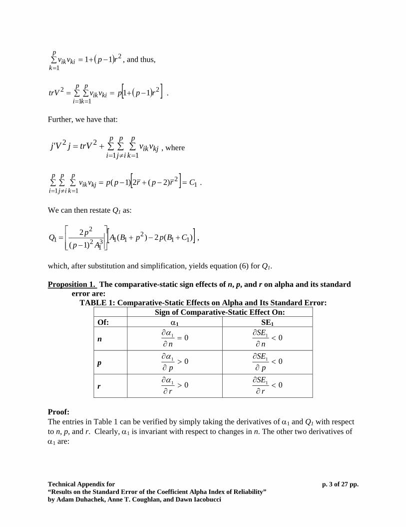
We can then restate Q1 as:

[ ])(2)()1(

211

2113

12

21 CBppBA

AppQ +−+

⎥⎥⎦

⎤

⎢⎢⎣

⎡

−= ,

which, after substitution and simplification, yields equation (6) for Q1. Proposition 1. The comparative-static sign effects of n, p, and r on alpha and its standard

error are: TABLE 1: Comparative-Static Effects on Alpha and Its Standard Error:

Sign of Comparative-Static Effect On: Of: α1 SE1

n 01 =∂∂

nα 01 <

∂∂

nSE

p 01 >∂∂

pα 01 <

∂∂

pSE

r 01 >∂∂

rα 01 <

∂∂

rSE

Proof: The entries in Table 1 can be verified by simply taking the derivatives of α1 and Q1 with respect to n, p, and r. Clearly, α1 is invariant with respect to changes in n. The other two derivatives of α1 are:


p. 3 of 27 pp.

( )( )[ ]

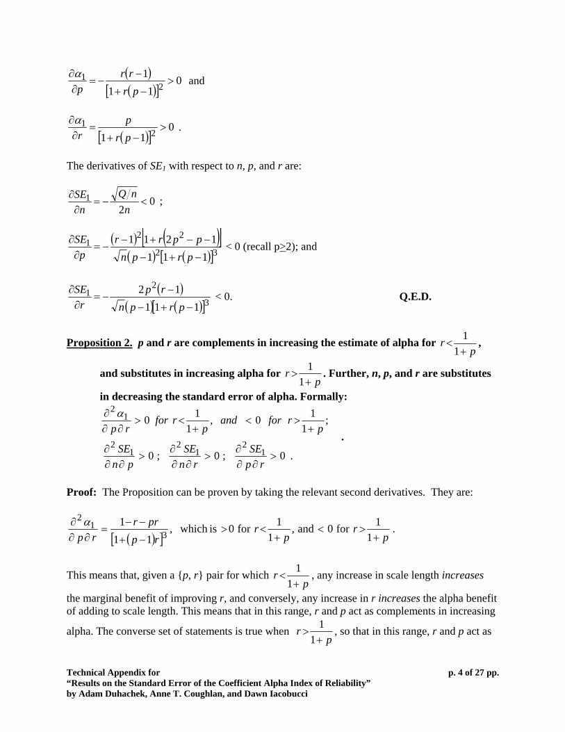
011

12

1 >−+

−−=

∂∂

prrr

pα and

( )[ ]0

11 21 >

−+=

∂∂

prp

rα .

The derivatives of SE1 with respect to n, p, and r are:

02

1 <−=∂∂

nnQ

nSE ;

( ) ( )[ ]

( ) ( )[ ]32

221

1111211

−+−

−−+−−=

∂∂

prpnpprr

pSE < 0 (recall p>2); and

( )( ) ( )[ ]3

21

11112−+−

−−=

∂∂

prpnrp

rSE < 0. Q.E.D.

Proposition 2. p and r are complements in increasing the estimate of alpha for p

r+

<1

1 ,

and substitutes in increasing alpha for p

r+

>1

1 . Further, n, p, and r are substitutes

in decreasing the standard error of alpha. Formally:

.0;0;0

;1

10,1

10

12

12

12

12

>∂∂

∂>

∂∂∂

>∂∂

∂

+><

+<>

∂∂∂

rpSE

rnSE

pnSE

prforand

prfor

rpα

.

Proof: The Proposition can be proven by taking the relevant second derivatives. They are:

( )[ ].

11for0 and,

11for0 iswhich ,

111

31

2

pr

pr

rpprr

rp +><

+<>

−+

−−=

∂∂∂ α

This means that, given a {p, r} pair for which p

r+

<1

1 , any increase in scale length increases

the marginal benefit of improving r, and conversely, any increase in r increases the alpha benefit of adding to scale length. This means that in this range, r and p act as complements in increasing

alpha. The converse set of statements is true when p

r+

>1

1 , so that in this range, r and p act as


p. 4 of 27 pp.

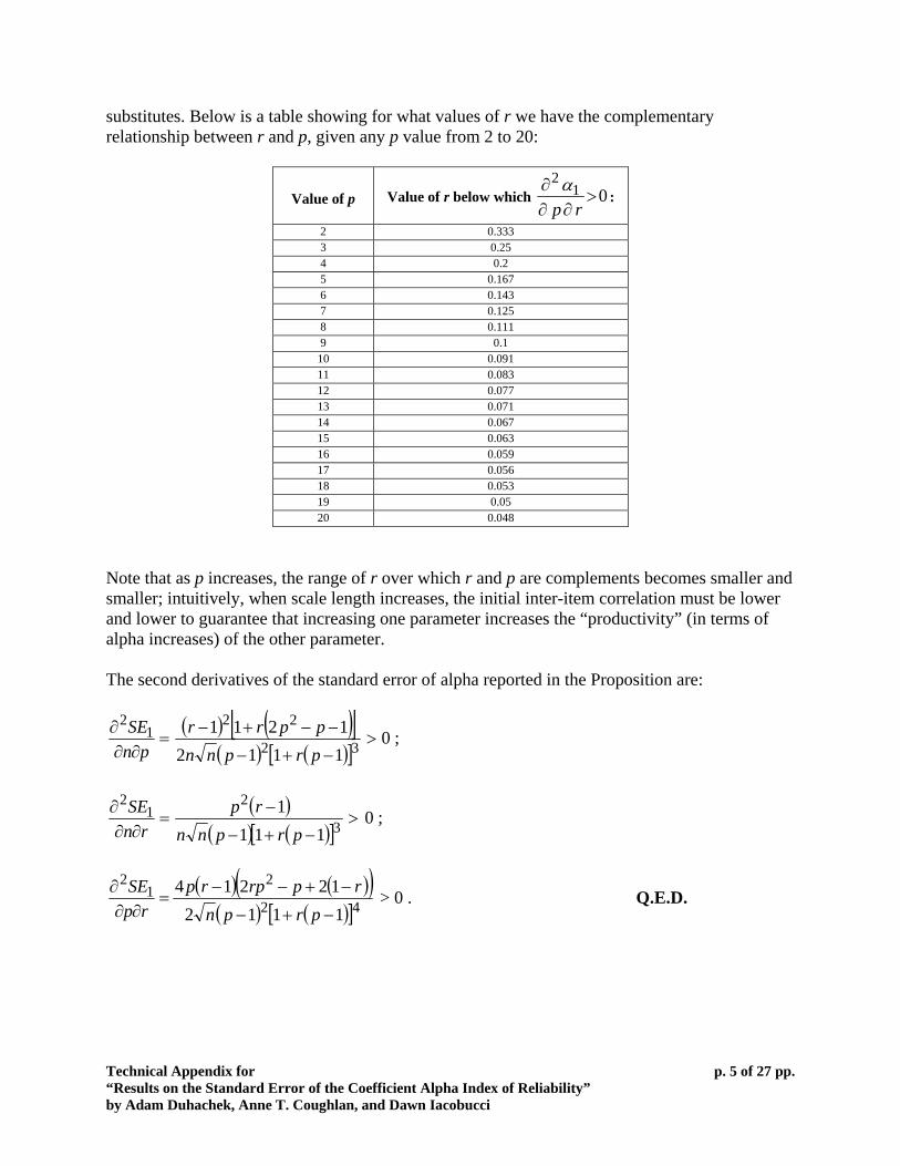
substitutes. Below is a table showing for what values of r we have the complementary relationship between r and p, given any p value from 2 to 20:

Value of p Value of r below which 012

>∂∂

∂rp

α:

2 0.333 3 0.25 4 0.2 5 0.167 6 0.143 7 0.125 8 0.111 9 0.1 10 0.091 11 0.083 12 0.077 13 0.071 14 0.067 15 0.063 16 0.059 17 0.056 18 0.053 19 0.05 20 0.048

Note that as p increases, the range of r over which r and p are complements becomes smaller and smaller; intuitively, when scale length increases, the initial inter-item correlation must be lower and lower to guarantee that increasing one parameter increases the “productivity” (in terms of alpha increases) of the other parameter. The second derivatives of the standard error of alpha reported in the Proposition are:

( ) ( )[ ]

( ) ( )[ ];0

11121211

32

221

2>

−+−

−−+−=

∂∂∂

prpnnpprr

pnSE

( )( ) ( )[ ]

;0111

13

21

2>

−+−

−=

∂∂∂

prpnnrp

rnSE

( ) ( )( )( ) ( )[ ]42

21

2

111212214−+−

−+−−=

∂∂∂

prpnrprprp

rpSE > 0 . Q.E.D.


p. 5 of 27 pp.

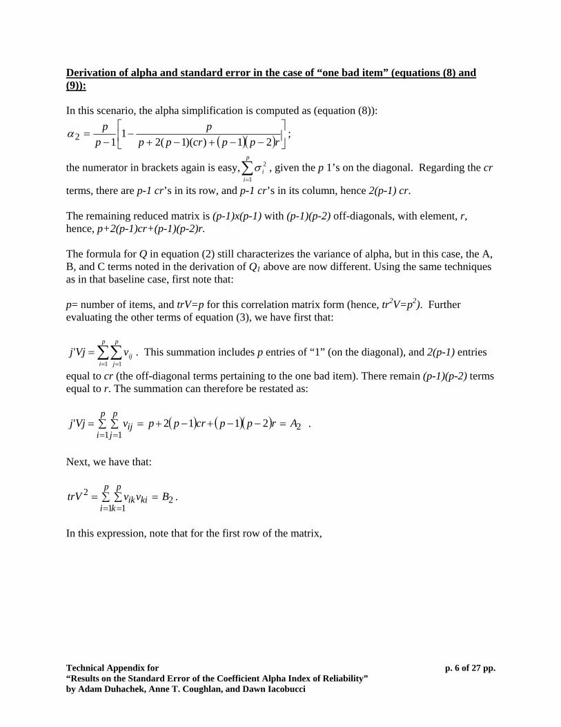
Derivation of alpha and standard error in the case of “one bad item” (equations (8) and (9)): In this scenario, the alpha simplification is computed as (equation (8)):

( )( ) ⎥⎦

⎤⎢⎣

⎡−−+−+

−−

=rppcrpp

pp

p21))(1(2

112α ;

the numerator in brackets again is easy, , given the p 1’s on the diagonal. Regarding the cr

terms, there are p-1 cr’s in its row, and p-1 cr’s in its column, hence 2(p-1) cr.

∑=

p

ii

1

2σ

The remaining reduced matrix is (p-1)x(p-1) with (p-1)(p-2) off-diagonals, with element, r, hence, p+2(p-1)cr+(p-1)(p-2)r. The formula for Q in equation (2) still characterizes the variance of alpha, but in this case, the A, B, and C terms noted in the derivation of Q1 above are now different. Using the same techniques as in that baseline case, first note that: p= number of items, and trV=p for this correlation matrix form (hence, tr2V=p2). Further evaluating the other terms of equation (3), we have first that:

∑∑= =

=p

i

p

jijvVjj

1 1' . This summation includes p entries of “1” (on the diagonal), and 2(p-1) entries

equal to cr (the off-diagonal terms pertaining to the one bad item). There remain (p-1)(p-2) terms equal to r. The summation can therefore be restated as:

( ) ( )( ) 21 1

2112' ArppcrppvVjjp

i

p

jij =−−+−+=∑ ∑=

= = .

Next, we have that:

21 1

2 BvvtrVp

i

p

kkiik =∑ ∑=

= =.

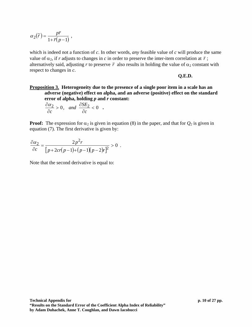
In this expression, note that for the first row of the matrix,


p. 6 of 27 pp.

( )( ) .11 2

111 crpvv

p

kkk −+=∑

=

For the next (p-1) rows, we have:

( ) ( ) ( )[ ] .211 22

11 rpcrpvv

p

kikiik −++−=∑

=≠

The sum can therefore be written as:

( )( ) ( ) ( ) ( )[ ] .21111 2222

1 1

2 rpcrpcrpBvvtrVp

i

p

kkiik −++−+−+==∑ ∑=

= =


∑ ∑ ∑+== ≠ =

p

i

p

ij

p

kkjikvvtrVjVj

1 1

22' , where through the same sort of calculation,

[ ] ( )( ) ( ) ( )[ ] 2222

1 13221)2(2)1(2 Crprcrppcrpcrpvv

p

i

p

ij

p

kkjik =−++−−+−+−=∑ ∑ ∑

= ≠ = .


[ ])(2)()1(

222

2223

22

22 CBppBA

AppQ +−+

⎥⎥⎦

⎤

⎢⎢⎣

⎡

−= ,

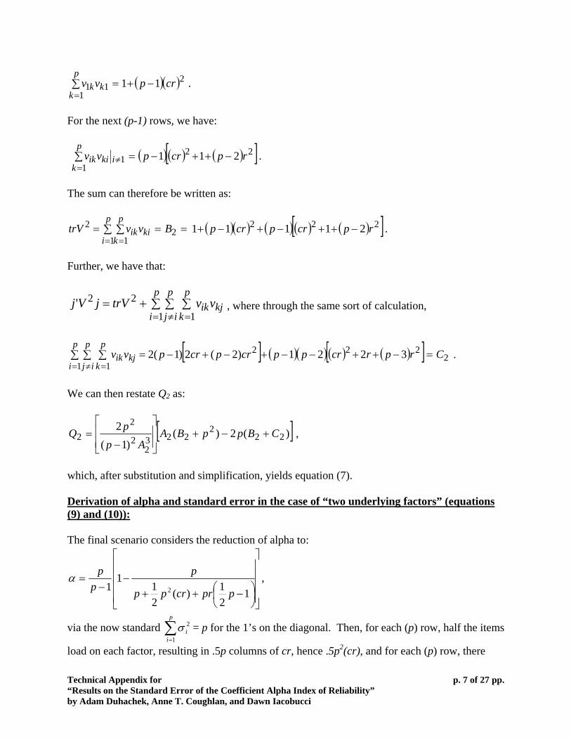
which, after substitution and simplification, yields equation (7). Derivation of alpha and standard error in the case of “two underlying factors” (equations (9) and (10)): The final scenario considers the reduction of alpha to:

⎥⎥⎥⎥

⎦

⎤

⎢⎢⎢⎢

⎣

⎡

⎟⎠⎞

⎜⎝⎛ −++

−−

=1

21)(

21

11 2 pprcrpp

pp

pα ,

via the now standard = p for the 1’s on the diagonal. Then, for each (p) row, half the items

load on each factor, resulting in .5p columns of cr, hence .5p

∑=

p

ii

1

2σ

2(cr), and for each (p) row, there


p. 7 of 27 pp.

exists an r in each location in the upper and lower submatrices, hence pr(.5p-1), altogether, p+.5p2cr+pr(.5p-1). The formula for Q in equation (2) still characterizes the variance of alpha, but in this case, the A, B, and C terms noted in the derivations of Q1 and Q2 above are different. Using the same techniques as in that baseline case, first note that: p= number of items, and trV=p for this correlation matrix form (hence, tr2V=p2). Further evaluating the other terms of equation (2), we have first that:

∑∑= =

=p

i

p

jijvVjj

1 1' . This summation includes p entries of “1” (on the diagonal). Further, in any of

the p rows of the matrix, half of the items load on each factor; so there are (.5p2) instances where an entry of (cr) occurs in the matrix. Finally, in each of the p rows of the matrix, there are entries of r in (.5p-1) cells, so across the whole matrix, there are [p(.5p-1)] instances of an entry of r. Thus, the summation can be written as:

( ) 32

1 115.5.' ApprcrppvVjj

p

i

p

jij =−++=∑ ∑=

= = .

For the next term,

31 1

2 BvvtrVp

i

p

kkiik =∑ ∑=

= =.

In this expression, note that for each row of the matrix,

( ) ( ) 22

111 15.5.1 rpcrpvv

p

kkk −++=∑

= ,

so that the entire term becomes

( ) ( )[ ] 32

1 1

2 15.5.1 BrpcrppvvtrVp

i

p

kkiik =−++=∑ ∑=

= = .


∑ ∑ ∑+== ≠ =

p

i

p

ij

p

kkjikvvtrVjVj

1 1

22' , where through the same sort of calculation,


p. 8 of 27 pp.

( ) ( ) ( )[ ] ( )[ ] 32222

1 1225.25.5.215. Ccrpcrprpcrprppvv

p

i

p

ij

p

kkjik =−++−++−=∑ ∑ ∑

= ≠ = .


[ ])(2)()1(

233

2333

32

23 CBppBA

AppQ +−+

⎥⎥⎦

⎤

⎢⎢⎣

⎡

−= ,

which, after substitution and simplification, yields equation (9). Demonstration that any combination of c and r that yields the same r yields the same alpha estimate (relevant for section on “Adding an Item to a Scale”): We show here that the same alpha value results from some r combined with c=1 (the baseline case), as from some c<1 combined with a higher r value, such that the average is still r . In other words, for any given p, any combination of c and r that yields the same r yields the same alpha estimate. The formula for α2 is given in equation (8). When there is “one bad item,” this means that there are (p-1) items that have intercorrelations equal to r, and one item that has a correlation of cr with each of the other items. In this case, it is straightforward to show that the average intercorrelation among the p items is given by:

( )p

cprr 22 −+= .

Note that in the special case where the starting point is our baseline case, c=1 and the above formula reduces to simply rr = , which is clearly true. In any other general starting situation, just as in the situation where the starting point is the baseline case, r is given and known, and hence can be treated as a parameter for the following discussion. Imagine now changing the value of c; how would r have to change as well, in such a way as to preserve r as the average inter-item correlation? This would imply that r, the underlying correlation among the first (p-1) items, has to adjust according to the following rule:

.~22

rcprpr =−+

=

To see what this adjustment rule implies for the value of alpha, we next substitute in r~ for r in the formula for α2, to get:


p. 9 of 27 pp.

( ) ( )11~

2 −+=

prrprα ,

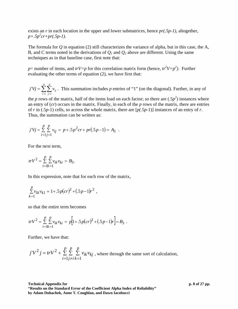
which is indeed not a function of c. In other words, any feasible value of c will produce the same value of α2, if r adjusts to changes in c in order to preserve the inter-item correlation at r ; alternatively said, adjusting r to preserve r also results in holding the value of α2 constant with respect to changes in c. Q.E.D. Proposition 3. Heterogeneity due to the presence of a single poor item in a scale has an

adverse (negative) effect on alpha, and an adverse (positive) effect on the standard error of alpha, holding p and r constant:

0,0 22 <∂

∂>

∂∂

cSEand

cα .

Proof: The expression for α2 is given in equation (8) in the paper, and that for Q2 is given in equation (7). The first derivative is given by:

( ) ( )( )[ ]0

21122

2

22 >

−−+−+=

∂∂

rpppcrprp

cα .

Note that the second derivative is equal to:


p. 10 of 27 pp.

cQ

nQcSE

∂∂

=∂

∂ 2

2

22

1 ,

whose sign is the sign of c

Q∂∂ 2 . This can be expressed as:

( ) ( ) ( ) ( )( )( ) ( ) ( )[ ]

( ) ( ) ([ ]( ) ( )[ ]

( ) ( )[ ] .012321

01111

432911351

8131991

56531214

08

,

42

4

32223

22

232

2

2

>−+−++=

>−=−−−−

+−+−−−−+−+

−+−−−−

−+−−−+−−=

>=

⋅⋅

=∂∂

crrcrprpD

pCrcrrp

rccrccrcp

rcrccrp

rcrccprrcB

rpA

whereDCBA

cQ

)

The sign of c

Q∂∂ 2 is therefore the sign of term B above. We can note immediately that B is a

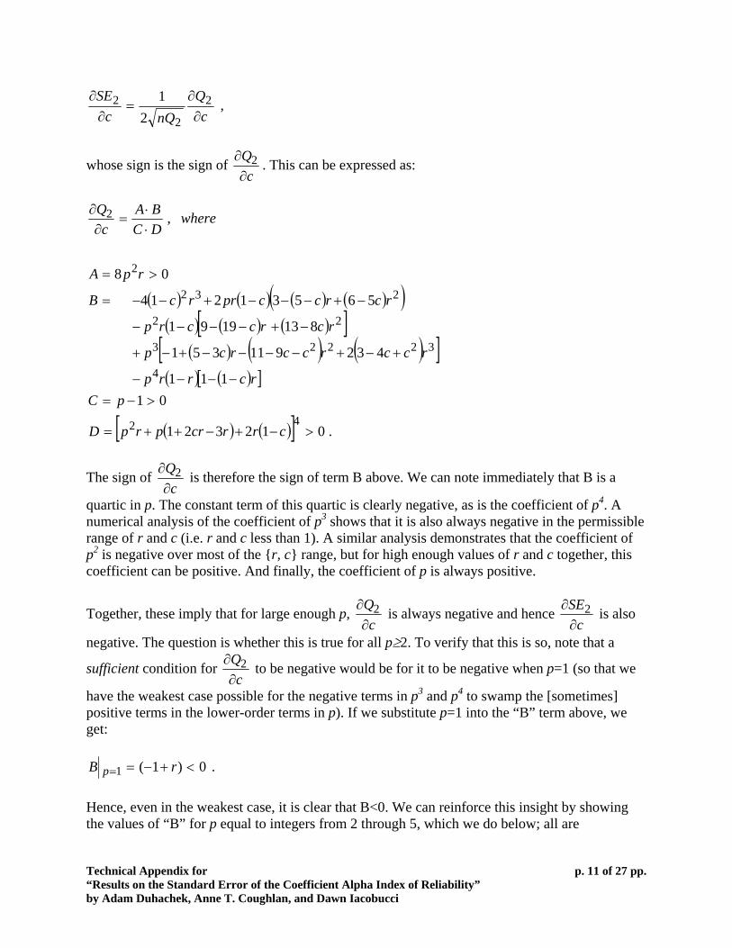
quartic in p. The constant term of this quartic is clearly negative, as is the coefficient of p4. A numerical analysis of the coefficient of p3 shows that it is also always negative in the permissible range of r and c (i.e. r and c less than 1). A similar analysis demonstrates that the coefficient of p2 is negative over most of the {r, c} range, but for high enough values of r and c together, this coefficient can be positive. And finally, the coefficient of p is always positive.

Together, these imply that for large enough p, c

Q∂∂ 2 is always negative and hence

cSE∂

∂ 2 is also

negative. The question is whether this is true for all p≥2. To verify that this is so, note that a

sufficient condition for c

Q∂∂ 2 to be negative would be for it to be negative when p=1 (so that we

have the weakest case possible for the negative terms in p3 and p4 to swamp the [sometimes] positive terms in the lower-order terms in p). If we substitute p=1 into the “B” term above, we get:

0)1(1 <+−== rB p .

Hence, even in the weakest case, it is clear that B<0. We can reinforce this insight by showing the values of “B” for p equal to integers from 2 through 5, which we do below; all are


p. 11 of 27 pp.

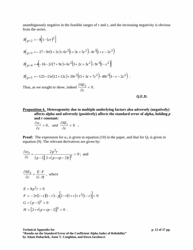
unambiguously negative in the feasible ranges of r and c, and the increasing negativity is obvious from the series.

( )[ ]22 18 crB p −−==

( ) ( ) ( )2322

3 214531621927 ccrccrcrB p −+−++++−−==

( ) ( ) ( )[ ]2322

4 193236972164 crccrcrB p −−++++−−==

( ) ( ) ( )2322

5 2348731520121215125 ccrccrcrB p −−−++++−−== .

Thus, as we sought to show, indeed 02 <∂

∂c

SE.

Q.E.D. Proposition 4. Heterogeneity due to multiple underlying factors also adversely (negatively)

affects alpha and adversely (positively) affects the standard error of alpha, holding p and r constant:

0,0 33 <∂∂

>∂∂

cSE

andcα .

Proof: The expression for α3 is given in equation (10) in the paper, and that for Q3 is given in equation (9). The relevant derivatives are given by:

( ) ( )[ ]0

2212

2

23 >

−++−=

∂∂

rcppprp

cα ; and

( )( ) ( ) ( )[ ]( )

( )[ ] .022

01

0112112

08

,

3

2

2

2

3

>−++=

>−=

<−++−−−−−=

>=

⋅⋅

=∂

∂

cpprH

pG

crcrprcrF

rpE

whereHGFE

cSE


p. 12 of 27 pp.

Thus, c

SE∂

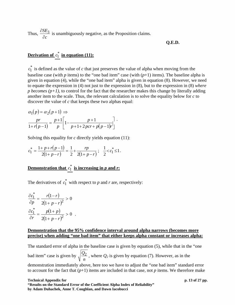
∂ 3 is unambiguously negative, as the Proposition claims.

Q.E.D. Derivation of *

1c in equation (11):

*1c is defined as the value of c that just preserves the value of alpha when moving from the

baseline case (with p items) to the “one bad item” case (with (p+1) items). The baseline alpha is given in equation (4), while the “one bad item” alpha is given in equation (8). However, we need to equate the expression in (4) not just to the expression in (8), but to the expression in (8) where p becomes (p+1), to control for the fact that the researcher makes this change by literally adding another item to the scale. Thus, the relevant calculation is to solve the equality below for c to discover the value of c that keeps these two alphas equal:

( ) ( )

( ) ( ) ⎥⎦

⎤⎢⎣

⎡−+++

+−

+=

−+

⇒+=

rpppcrpp

pp

prpr

pp

121111

11

121 αα .

Solving this equality for c directly yields equation (11):

( )( ) ( ) 1

21;

1221

1211 *

1*1 ≤<

−++=

−+−++

= crp

rprp

prpc .

Demonstration that *

1c is increasing in p and r: The derivatives of with respect to p and r are, respectively: *

1c

( )( )

012

12

*1 >

−+

−=

∂∂

rprr

pc

( )( )

012

12

*1 >

−+

+=

∂∂

rppp

rc .

Demonstration that the 95% confidence interval around alpha narrows (becomes more precise) when adding “one bad item” that either keeps alpha constant or increases alpha: The standard error of alpha in the baseline case is given by equation (5), while that in the “one

bad item” case is given by n

Q2 , where Q2 is given by equation (7). However, as in the

demonstration immediately above, here too we have to adjust the “one bad item” standard error to account for the fact that (p+1) items are included in that case, not p items. We therefore make


p. 13 of 27 pp.

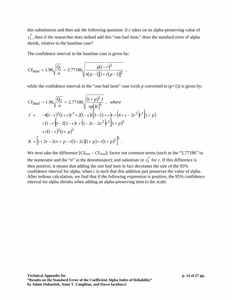
this substitution and then ask the following question: if c takes on its alpha-preserving value of , then if the researcher does indeed add this “one bad item,” does the standard error of alpha

shrink, relative to the baseline case?

*1c

The confidence interval in the baseline case is given by:

( )( ) ( )[ ]2

21

111177186.296.1

−+−

−==

prpnrp

nQCIbase ,

while the confidence interval in the “one bad item” case (with p converted to (p+1)) is given by:

( )[ ]

( ) ( ) ( ) ( ) ( )[ ]( )( ) ( ) ( )[ ]( )( ) ( )

( )( ) ( )[ ] .1123221

11

12252211

1245312114

,177186.296.1

32

32

222

2232

3

22

1

prpcrpcrrK

prr

prccrcr

prccrcrcrccJ

whereKnp

Jpn

QCI bad

+++−−+−+=

+−+

+−−+−−−+

+−+++−−++−−=

+==

We next take the difference [CIbase – CI1bad]; factor out common terms (such as the “2.77186” in the numerator and the “n” in the denominator); and substitute in for c. If this difference is then positive, it means that adding the one bad item in fact decreases the size of the 95% confidence interval for alpha, when c is such that this addition just preserves the value of alpha. After tedious calculation, we find that if the following expression is positive, the 95% confidence interval for alpha shrinks when adding an alpha-preserving item to the scale:

*1c


p. 14 of 27 pp.

( )( ) ( )[ ]( ) ( ) ( )( ) ( ) ([ ]

( ) ( )[ ]) .

11123222112121

1111

32

33322332

2

2

−++

+−+−+−++−++−−

−+−

−=

prpppprppprpprpr

prprpCIdiffsign

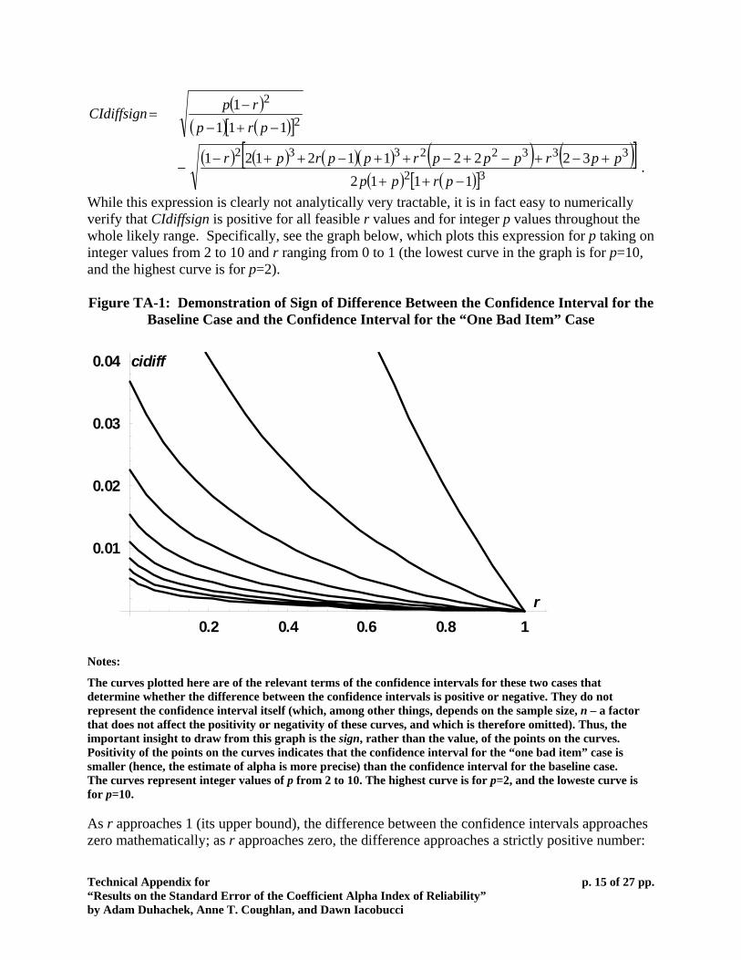
While this expression is clearly not analytically very tractable, it is in fact easy to numerically verify that CIdiffsign is positive for all feasible r values and for integer p values throughout the whole likely range. Specifically, see the graph below, which plots this expression for p taking on integer values from 2 to 10 and r ranging from 0 to 1 (the lowest curve in the graph is for p=10, and the highest curve is for p=2). Figure TA-1: Demonstration of Sign of Difference Between the Confidence Interval for the

Baseline Case and the Confidence Interval for the “One Bad Item” Case

0.2 0.4 0.6 0.8 1

0.01

0.02

0.03

0.04

r

cidiff

Notes:

The curves plotted here are of the relevant terms of the confidence intervals for these two cases that determine whether the difference between the confidence intervals is positive or negative. They do not represent the confidence interval itself (which, among other things, depends on the sample size, n – a factor that does not affect the positivity or negativity of these curves, and which is therefore omitted). Thus, the important insight to draw from this graph is the sign, rather than the value, of the points on the curves. Positivity of the points on the curves indicates that the confidence interval for the “one bad item” case is smaller (hence, the estimate of alpha is more precise) than the confidence interval for the baseline case. The curves represent integer values of p from 2 to 10. The highest curve is for p=2, and the loweste curve is for p=10. As r approaches 1 (its upper bound), the difference between the confidence intervals approaches zero mathematically; as r approaches zero, the difference approaches a strictly positive number:


p. 15 of 27 pp.

( )1122

−−−

pppp

. As p approaches infinity, the difference between the confidence intervals

mathematically approaches zero; but as the graph above indicates, finite values of p imply that the confidence interval for the baseline case is strictly greater in size than for the “one bad item” case (and therefore, adding one bad item that just preserves the value of alpha also makes that estimate more precise). By extension, adding “one bad item” that actually increases the alpha estimate will also tighten the 95% confidence interval. The remainder of these results supplement the article: Derivation of *

2c :

*2c is defined as the value of c that just preserves the value of alpha when moving from the

baseline case (with p items) to the “two underlying factors” case (with (p+2) items). The baseline alpha is given in equation (5), while the “two underlying factors” alpha is given in equation (10). However, we need to equate the expression in (5) not just to the expression in (10), but to the expression in (10) where p becomes (p+2), to control for the fact that the researcher makes this change by literally adding two more items to the scale. Thus, the relevant calculation is to solve the equality below for c to discover the value of c that keeps these two alphas equal:

( ) ( )

( )( ) ( )[ ]

( ) ([ ])22122

11

231

+++++++

=−+

⇒+=

pcrprppcppr

prpr

pp αα .

Solving this equality for c directly yields:

( )( )( ) .1;

2222 *

2*2 ≤

+−++

= cprp

prpc

Demonstration that *

2c is increasing in p and r: The derivatives of *

2c with respect to p and r are, respectively:

( )( )( ) ( )

0222

221422

2*2 >

−++

++−=

∂∂

rpprppr

pc

( )( )( )

0222

142

*1 >

−++

+=

∂∂

rpppp

rc .


p. 16 of 27 pp.

Calculations Showing When Moving From the Baseline Case to the “Two Underlying Factors” Case Decreases the Size of the 95% Confidence Interval: Moving from the baseline case to the “two underlying factors” case may or may not improve the precision of the alpha estimate. To establish this, we first subtract the expression for the 95% confidence interval in the “two underlying factors” case from that in the baseline case, in the same fashion as we did above when comparing the baseline case to the “one bad item” case, assuming that c = . *

2c The confidence interval in the baseline case is given by:

( )( ) ( )[ ]2

21

111177186.296.1

−+−

−==

prpnrp

nQCIbase ,

while the confidence interval in the “two underlying factors” case (with p converted to (p+2)) is given by:

( ) ( ) ( ) ( )[ ]{ }( ) ( )[ ]22

2222

221112212292.3

++++

+++−+−+=

pcrprpncrcrpcrpCI factor .

Now suppose that c = ; under what conditions then does adding two items to a baseline scale to create a scale with two underlying factors nevertheless tighten up the 95% confidence interval? To answer this, we substitute in for c above and set the two confidence interval expressions equal to each other. After accounting for common terms, a sufficient condition for the 95% confidence interval to shrink in this situation is that the expression CIdiffsign2 below be positive:

*2c

*2c

( )( )( )2

322

216348

12

++

++++−

−=

pppprp

ppCIdiffsign .

This can be straightforwardly solved for r to show that, when c = , adding the two items shrinks the 95% confidence interval as long as:

*2c

( )( )12

2−

+<

pppr .

The Table below reports values of r (given values of p) above which the 95% confidence interval around alpha actually gets larger (i.e., for which the estimate of alpha is less precise) when the researcher adds two items to a baseline scale to create a “two underlying factors” scale:


p. 17 of 27 pp.

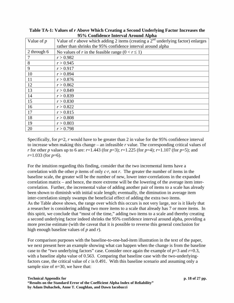
Table TA-1: Values of r Above Which Creating a Second Underlying Factor Increases the 95% Confidence Interval Around Alpha

Value of p Value of r above which adding 2 items (creating a 2nd underlying factor) enlarges rather than shrinks the 95% confidence interval around alpha

2 through 6 No values of r in the feasible range (0 < r ≤ 1) 7 r > 0.982 8 r > 0.945 9 r > 0.917 10 r > 0.894 11 r > 0.876 12 r > 0.862 13 r > 0.849 14 r > 0.839 15 r > 0.830 16 r > 0.822 17 r > 0.815 18 r > 0.808 19 r > 0.803 20 r > 0.798 Specifically, for p=2, r would have to be greater than 2 in value for the 95% confidence interval to increase when making this change – an infeasible r value. The corresponding critical values of r for other p values up to 6 are: r=1.443 (for p=3); r=1.225 (for p=4); r=1.107 (for p=5); and r=1.033 (for p=6). For the intuition regarding this finding, consider that the two incremental items have a correlation with the other p items of only c⋅r, not r. The greater the number of items in the baseline scale, the greater will be the number of new, lower inter-correlations in the expanded correlation matrix – and hence, the more extreme will be the lowering of the average item inter-correlation. Further, the incremental value of adding another pair of items to a scale has already been shown to diminish with initial scale length; eventually, the diminution in average item inter-correlation simply swamps the beneficial effect of adding the extra two items. As the Table above shows, the range over which this occurs is not very large, nor is it likely that a researcher is considering adding two more items to a scale that already has 7 or more items. In this spirit, we conclude that “most of the time,” adding two items to a scale and thereby creating a second underlying factor indeed shrinks the 95% confidence interval around alpha, providing a more precise estimate (with the caveat that it is possible to reverse this general conclusion for high enough baseline values of p and r). For comparison purposes with the baseline-to-one-bad-item illustration in the text of the paper, we next present here an example showing what can happen when the change is from the baseline case to the “two underlying factors” case. Consider once again the example of p=3 and r=0.3, with a baseline alpha value of 0.563. Comparing that baseline case with the two-underlying-factors case, the critical value of c is 0.491. With this baseline scenario and assuming only a sample size of n=30, we have that:


p. 18 of 27 pp.

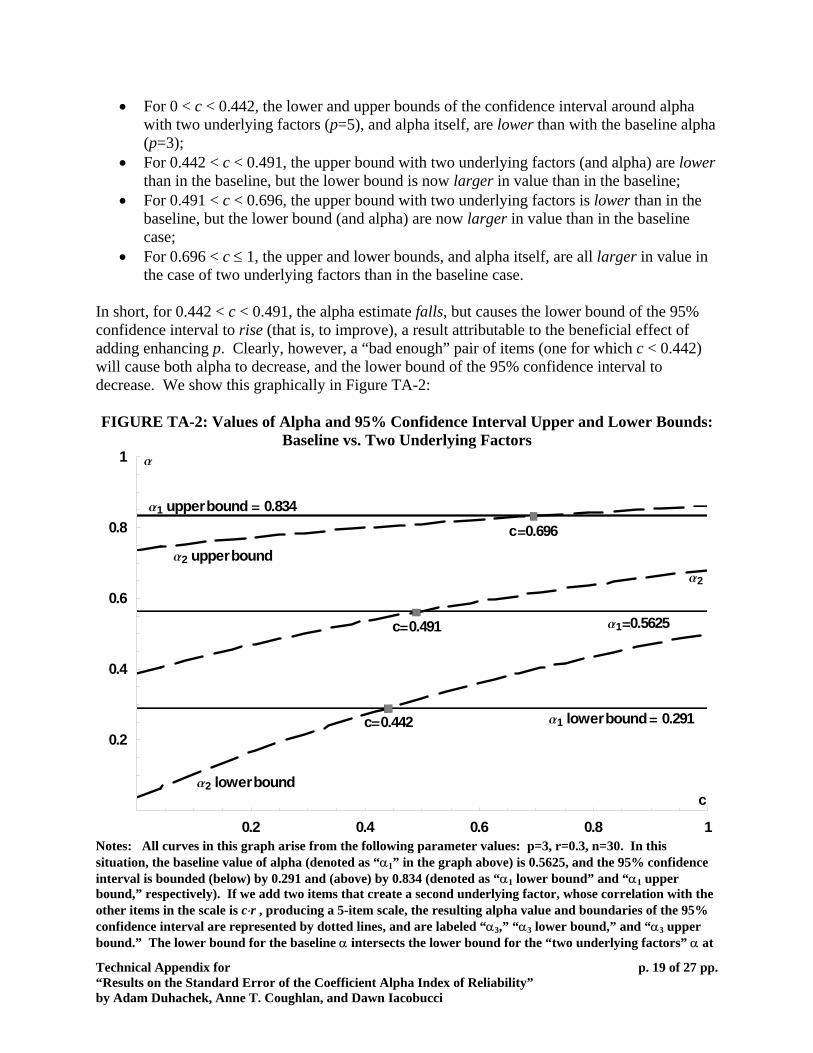
• For 0 < c < 0.442, the lower and upper bounds of the confidence interval around alpha with two underlying factors (p=5), and alpha itself, are lower than with the baseline alpha (p=3);

• For 0.442 < c < 0.491, the upper bound with two underlying factors (and alpha) are lower than in the baseline, but the lower bound is now larger in value than in the baseline;

• For 0.491 < c < 0.696, the upper bound with two underlying factors is lower than in the baseline, but the lower bound (and alpha) are now larger in value than in the baseline case;

• For 0.696 < c ≤ 1, the upper and lower bounds, and alpha itself, are all larger in value in the case of two underlying factors than in the baseline case.

In short, for 0.442 < c < 0.491, the alpha estimate falls, but causes the lower bound of the 95% confidence interval to rise (that is, to improve), a result attributable to the beneficial effect of adding enhancing p. Clearly, however, a “bad enough” pair of items (one for which c < 0.442) will cause both alpha to decrease, and the lower bound of the 95% confidence interval to decrease. We show this graphically in Figure TA-2: FIGURE TA-2: Values of Alpha and 95% Confidence Interval Upper and Lower Bounds:

Baseline vs. Two Underlying Factors

0.2 0.4 0.6 0.8 1

0.2

0.4

0.6

0.8

1

a1=0.5625

a1 upperbound = 0.834

a1 lowerbound= 0.291

a2

a2 upperbound

a2 lowerbound

c=0.442

c=0.491

c=0.696

c

a

Notes: All curves in this graph arise from the following parameter values: p=3, r=0.3, n=30. In this situation, the baseline value of alpha (denoted as “α1” in the graph above) is 0.5625, and the 95% confidence interval is bounded (below) by 0.291 and (above) by 0.834 (denoted as “α1 lower bound” and “α1 upper bound,” respectively). If we add two items that create a second underlying factor, whose correlation with the other items in the scale is c⋅r , producing a 5-item scale, the resulting alpha value and boundaries of the 95% confidence interval are represented by dotted lines, and are labeled “α3,” “α3 lower bound,” and “α3 upper bound.” The lower bound for the baseline α intersects the lower bound for the “two underlying factors” α at


p. 19 of 27 pp.

c = 0.442. The α estimate for the baseline α intersects that for “two underlying factors” at c = 0.491. The upper bound for the baseline α intersects the upper bound for the “two underlying factors” α at c = 0.696.

Derivation of *3c :

*3c is defined as the value of c that just preserves the value of alpha when moving from the “one

bad item” case (with (p+1) items) to the “two underlying factors” case (with (p+2) items). The “one bad item” alpha is given in equation (8), while the “two underlying factors” alpha is given in equation (10). However, we need to adjust both alpha expressions to reflect the fact that the number of items is (p+1) in the “one bad item” case, and (p+2) in the “two underlying factors” case. Thus, the relevant calculation is to solve the equality below for c to discover the value of c that keeps these two alphas equal:

( ) ( )

( )( ) ( )[ ]

( ) ([ ])22122

121111

21 32

+++++++

=⎥⎦

⎤⎢⎣

⎡−+++

+−

+

⇒+=+

pcrprppcppr

rpppcrpp

pp

pp αα .

After algebraic manipulation, the two alpha expressions are equal if the expression Z below is zero (and the “two underlying factors” alpha is larger than the “one bad item” alpha if Z is positive):

( ) ( ) ( )[ ] ( ) ( )[ ]32222 14223122 prprppprppcprcZ −−++++−+−+++−=

Z is a quadratic in c. This quadratic approaches negative infinity as c approaches either negative infinity or positive infinity. Further, Z is clearly positive when c=1:

( )( )21 112 +−== prZ c .

Thus, the function Z does have a positive range, and this range does include at least one feasible c value. But Z is not always positive for all c values. Consider c=0, the other limit of the range of c. We have:

( ) ( ) 320 142 prprpZ c −−+++== .

Note that when c=0, Z is positive for p=2 (it equals (6-2r)), but is negative for p=3 (it then equals (-4-6r)). This suggests that when c is low, the alpha of an already-long scale is not enhanced by the addition of one more item that creates a second underlying factor.

We can solve for the two c roots of the Z expression above. One of the roots is always greater than 1 in value, and this (larger) root is the critical value of c above which Z is always negative. But the smaller c root is sometimes between 0 and 1 in value, and it is this smaller c root that is given by : *

3c


p. 20 of 27 pp.

( ) ( ) ( ) ( )( )pr

ppprpprpppprc

+

⎥⎦⎤

⎢⎣⎡ −−+−+−−++−+−

=24

168622123 2342222*3 .

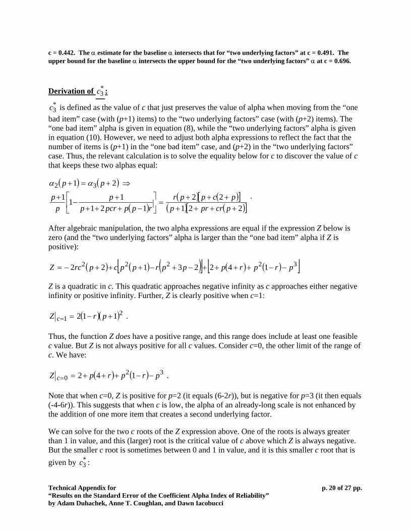
We show these critical values of c, as functions of r, for several salient values of p in Figure TA-3 below. Note that is increasing in r for any value of (p+1) greater than 3, and is similarly increasing in p for any value of r in these parameter ranges. Thus, it exhibits the same comparative-static properties as did and . Further, note that when the researcher starts with 3 items in the “one bad item” scale [i.e., (p+1)=3], it is always alpha-improving to add the incremental item (we therefore omit this case from the Figure). However, for any higher value of p, there exist {r, c} pairs for which it does not increase alpha to add the incremental item. As p increases, the minimum hurdle that c must surpass in order to increase alpha increases, just as it did in the first two illustrations. In the limit, as p approaches infinity, approaches 1. Thus in the limit, it is impossible to add one more item to a scale that increases the estimate of alpha.

*3c

*1c *

2c

*3c

FIGURE TA-3: Critical Values of c Above Which Alpha Increases

When Moving from “One Bad Item” to “Two Underlying Factors” Cases

0.2 0.4 0.6 0.8 1

0.2

0.4

0.6

0.8

1

p=3

p=5p=7p=9

p=11

r

Crit. c value


p. 21 of 27 pp.

Notes: When p=2, alpha increases when moving from “one bad item” (p=3) to “two underlying factors” (p=4) case, for all feasible values of c and r (c ∈ (0,1], r ∈ (0,1]). Each curve represents the value of c, for any value of r, that just holds alpha constant when moving from the “one bad item” case to the “two underlying factors” case, for each value of p.

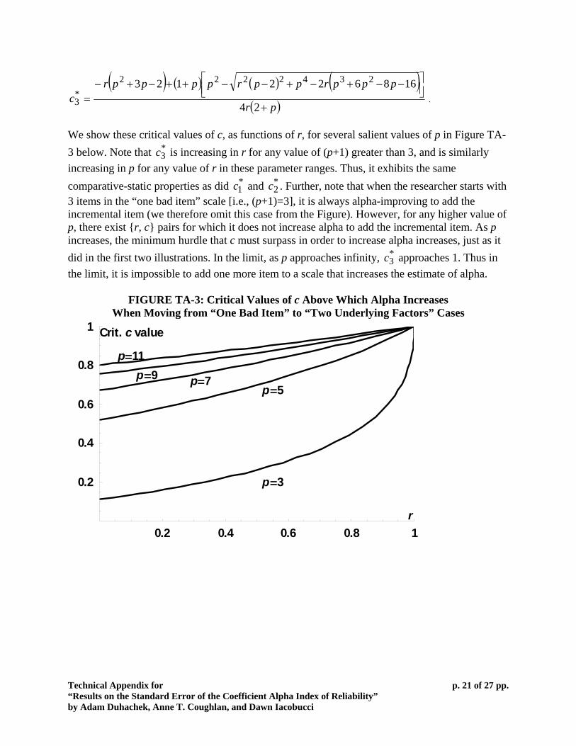
Demonstrating that Moving From the “One Bad Item” Case to the “Two Underlying Factors” Case Does Not Always Improve the 95% Confidence Interval, Even When Alpha Itself Remains Constant: Adding an incremental item in this third illustration does not always tighten the confidence interval around alpha, even when the estimate of alpha itself remains constant. A sufficiently low value of r (given p) guarantees that adding the incremental item decreases the variance around alpha, however. It is in these relatively low-r cases that adding another item, even one that creates a second underlying factor, has a chance of improving the precision of the estimate of alpha. The formula governing this relationship is not simple, so we present Table TA-2 here to illustrate the critical values of r for each value of p, under the assumption that the value of c is such as to keep the estimate of alpha itself constant:

TABLE TA-2: Values of r and c That Preserve Both Alpha and Its 95% Confidence Interval, Moving from “One Bad Item” Case to “Two Underlying Factors” Case, For

Various p Values

Value of p

Value of r that preserves the size of 95%

confidence interval (for c = alpha-preserving c

value) Value of c that preserves

alpha Implied (Constant)

Alpha Value

2 0.5 N/A (any c ∈ (0, 1] increases alpha) N/A

3 0.523810 0.272727 0.666667 4 0.590909 0.615385 0.833333 5 0.650000 0.769231 0.900000 6 0.696970 0.847826 0.933333 7 0.733990 0.892617 0.952381 8 0.763514 0.920354 0.964286 9 0.787440 0.938650 0.972222 10 0.807143 0.951327 0.977778 11 0.823609 0.960461 0.981818 12 0.837553 0.967254 0.984848 13 0.849498 0.972441 0.987179 100 0.980008 0.999592 0.999798

To illustrate, imagine p=3; i.e., the researcher is considering switching from a “one bad item” case with 4 items in it [(p+1) items] to a “two underlying factors” case with 5 items in it [(p+2) items]. In order for adding that incremental (p+2) item to make the estimate of alpha more precise, given a c value of 0.272727 (with this change preserving alpha), the underlying Technical Appendix for “Results on the Standard Error of the Coefficient Alpha Index of Reliability” by Adam Duhachek, Anne T. Coughlan, and Dawn Iacobucci

p. 22 of 27 pp.

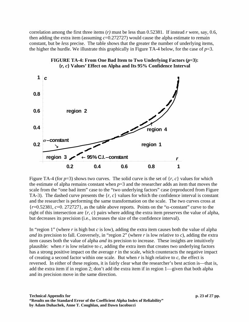
correlation among the first three items (r) must be less than 0.52381. If instead r were, say, 0.6, then adding the extra item (assuming c=0.272727) would cause the alpha estimate to remain constant, but be less precise. The table shows that the greater the number of underlying items, the higher the hurdle. We illustrate this graphically in Figure TA-4 below, for the case of p=3.

FIGURE TA-4: From One Bad Item to Two Underlying Factors (p=3): {r, c} Values’ Effect on Alpha and Its 95% Confidence Interval

0.2 0.4 0.6 0.8 1

0.2

0.4

0.6

0.8

1

r

c

a-constantä

95% C.I.-constant¨

region 1

region 2

region 3

region 4≠

Figure TA-4 (for p=3) shows two curves. The solid curve is the set of {r, c} values for which the estimate of alpha remains constant when p=3 and the researcher adds an item that moves the scale from the “one bad item” case to the “two underlying factors” case (reproduced from Figure TA-3). The dashed curve presents the {r, c} values for which the confidence interval is constant and the researcher is performing the same transformation on the scale. The two curves cross at {r=0.52381, c=0. 272727}, as the table above reports. Points on the “α-constant” curve to the right of this intersection are {r, c} pairs where adding the extra item preserves the value of alpha, but decreases its precision (i.e., increases the size of the confidence interval). In “region 1” (where r is high but c is low), adding the extra item causes both the value of alpha and its precision to fall. Conversely, in “region 2” (where r is low relative to c), adding the extra item causes both the value of alpha and its precision to increase. These insights are intuitively plausible: when r is low relative to c, adding the extra item that creates two underlying factors has a strong positive impact on the average r in the scale, which counteracts the negative impact of creating a second factor within one scale. But when r is high relative to c, the effect is reversed. In either of these regions, it is fairly clear what the researcher’s best action is—that is, add the extra item if in region 2; don’t add the extra item if in region 1—given that both alpha and its precision move in the same direction.


p. 23 of 27 pp.

But in “region 3” and “region 4,” the effect on alpha and its precision are not of the same directionality. In “region 3” (low r and low c), adding the extra item lowers alpha, but makes the estimate more precise. In “region 4” (high r and intermediate c), adding the item increases alpha, but makes the estimate less precise. Thus, the impact of adding an item to a scale is not fully revealed by merely assessing its effect on the estimate of alpha itself. The decision made by the researcher of course also rests upon the actual value of alpha derived in these cases, an issue we consider in the next section. In sum, in this illustration we consider the effect of moving from (p+1) to (p+2) items in a scale. In the (p+1)-item case, the scale contains one bad item. In the (p+2)-item case, the scale is made up of two underlying factors. The question considered is when and whether adding the (p+2) item to the scale improves the reliability of the scale. We show here that doing so can improve the estimate of alpha, if the underlying correlation among the first p items is low enough relative to the c factor characterizing the last two items added. Intuitively, the last item must not drag down the average correlation too much; but on the other hand, lengthening a scale always has a positive impact of its own. It is the counterbalancing of these effects that determines the net effect on alpha. However, in this illustration we also show that an increase in alpha is not necessarily accompanied by an increase in its precision. When the underlying correlation among the original p items is high, adding the incremental item may increase alpha but also increase the size of the confidence interval – that is, decrease its precision. In a situation like this, the researcher has to decide whether adding the extra item is “worth it,” which is a choice between the improvement in the mean estimate of alpha and the possibility (revealed through the confidence interval) that alpha could be lower. Demonstration of Result 1: When the researcher’s goal is to maximize the size of alpha and the initial scale has 3 items, the equilibrium number of items is:

• the baseline 3 items, if the {r, c} pair lies in either “region 1” or “region 2” of Figure 2;

• the “two underlying factors” 5-item scale if the {r, c} pair lies in either “region 3” or “region 4” of Figure 2.

In “region 1” of Figure 2, with very low c values and a range of low to high r values, the researcher is best off staying with the baseline set of 3 items in the scale. Adding one “bad” item does not improve alpha (the points in region 1 lie below the top curve); adding two items to move from the baseline case to the “two underlying factors” case also does not improve the value of alpha (the points in region 1 lie below the middle curve). And, if the researcher were in the “one bad item” case, it would not improve alpha to add another item that creates a “two underlying factors” case; conversely, it would improve alpha to drop the one bad item. The unique equilibrium number of items in this situation is therefore three in region 1. In “region 2” of Figure 2, if the researcher already has “one bad item” in a 4-item scale, alpha will improve with the fifth item that transforms the scale into a “two underlying factors” scale. However, it is not an equilibrium to have these five items in the scale, because these points lie below the “Illust. 2” curve in Figure 2. Alpha is higher for the baseline case of 3 items than it is for the 4-item scale with “one bad item” as well (since the points in region 2 lie below the “Illust.


p. 24 of 27 pp.

1” curve in Figure 2). Hence, in “region 2” we also find that the alpha-maximizing scale length is three. In “region 3” of Figure 2, moving from the baseline case to “one bad item” decreases alpha, but moving from the baseline case to “two underlying factors” increases alpha. Further, if the researcher starts with the “one bad item” case, alpha improves with the addition of one more item that transforms the scale into a “two underlying items” scale. Thus, the unique equilibrium number of items in “region 3” is five, with two underlying factors. Finally, in “region 4” of Figure 2, we have {r, c} pairs for which moving from the baseline case to the “one bad item” case improves alpha; moving from the baseline case to the “two underlying factors” case improves alpha; and moving from the “one bad item” case to the “two underlying factors” case also improves alpha. The unique equilibrium in this portion of the space is therefore also to have a 5-item scale, with two underlying factors. In sum, for the case of p=3, we see that the equilibrium number of factors is either the baseline 3 items (if the {r, c} pair lies in either “region 1” or “region 2”), or the “two underlying factors” 5-item scale (if the {r, c} pair lies in either “region 3” or “region 4”). It is never an equilibrium in this situation to add just one bad item to the baseline scale, given the opportunity to add another item that creates a second underlying factor. The intuition for the results rests on the relative size of c and r, given the low number of original items in the scale (p=3). When c is high enough relative to r, the beneficial effect of adding items swamps the negative effect of creating a scale with two underlying factors. But if c is too low relative to r, the researcher is best off sticking with the original 3-item scale. More generally, the implication is that when starting with a small number of items, adding as many items as possible is likely to be a good strategy for increasing the estimate of alpha.

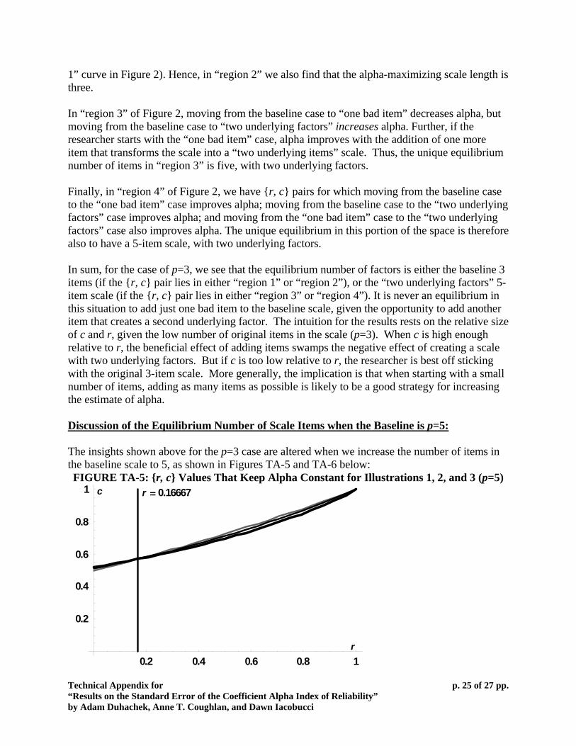
Discussion of the Equilibrium Number of Scale Items when the Baseline is p=5: The insights shown above for the p=3 case are altered when we increase the number of items in the baseline scale to 5, as shown in Figures TA-5 and TA-6 below: FIGURE TA-5: {r, c} Values That Keep Alpha Constant for Illustrations 1, 2, and 3 (p=5)

0.2 0.4 0.6 0.8 1

0.2

0.4

0.6

0.8

1

r

c r = 0.16667


p. 25 of 27 pp.

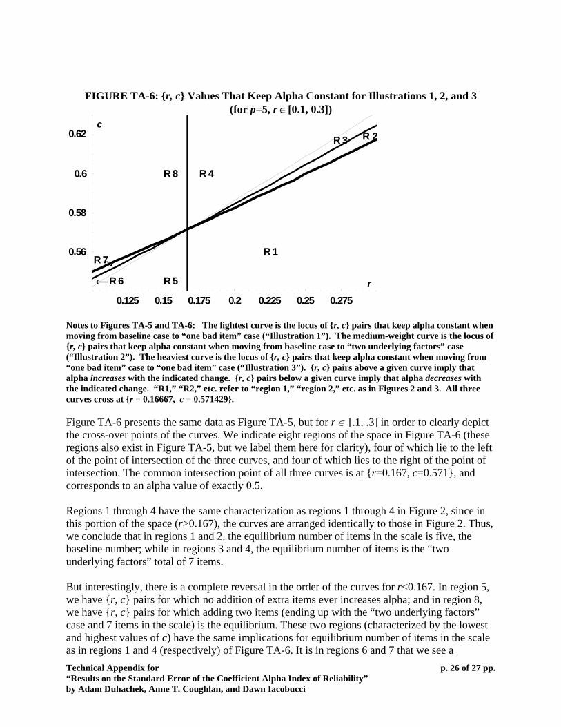
FIGURE TA-6: {r, c} Values That Keep Alpha Constant for Illustrations 1, 2, and 3 (for p=5, r ∈[0.1, 0.3])

0.125 0.15 0.175 0.2 0.225 0.25 0.275

0.56

0.58

0.6

0.62

r

c

R 1

R 2R 3

R 4

R 5R 6ò

R 7ä

R 8

Notes to Figures TA-5 and TA-6: The lightest curve is the locus of {r, c} pairs that keep alpha constant when moving from baseline case to “one bad item” case (“Illustration 1”). The medium-weight curve is the locus of {r, c} pairs that keep alpha constant when moving from baseline case to “two underlying factors” case (“Illustration 2”). The heaviest curve is the locus of {r, c} pairs that keep alpha constant when moving from “one bad item” case to “one bad item” case (“Illustration 3”). {r, c} pairs above a given curve imply that alpha increases with the indicated change. {r, c} pairs below a given curve imply that alpha decreases with the indicated change. “R1,” “R2,” etc. refer to “region 1,” “region 2,” etc. as in Figures 2 and 3. All three curves cross at {r = 0.16667, c = 0.571429}.

Figure TA-6 presents the same data as Figure TA-5, but for r ∈ [.1, .3] in order to clearly depict the cross-over points of the curves. We indicate eight regions of the space in Figure TA-6 (these regions also exist in Figure TA-5, but we label them here for clarity), four of which lie to the left of the point of intersection of the three curves, and four of which lies to the right of the point of intersection. The common intersection point of all three curves is at {r=0.167, c=0.571}, and corresponds to an alpha value of exactly 0.5. Regions 1 through 4 have the same characterization as regions 1 through 4 in Figure 2, since in this portion of the space (r>0.167), the curves are arranged identically to those in Figure 2. Thus, we conclude that in regions 1 and 2, the equilibrium number of items in the scale is five, the baseline number; while in regions 3 and 4, the equilibrium number of items is the “two underlying factors” total of 7 items. But interestingly, there is a complete reversal in the order of the curves for r<0.167. In region 5, we have {r, c} pairs for which no addition of extra items ever increases alpha; and in region 8, we have {r, c} pairs for which adding two items (ending up with the “two underlying factors” case and 7 items in the scale) is the equilibrium. These two regions (characterized by the lowest and highest values of c) have the same implications for equilibrium number of items in the scale as in regions 1 and 4 (respectively) of Figure TA-6. It is in regions 6 and 7 that we see a Technical Appendix for “Results on the Standard Error of the Coefficient Alpha Index of Reliability” by Adam Duhachek, Anne T. Coughlan, and Dawn Iacobucci

p. 26 of 27 pp.

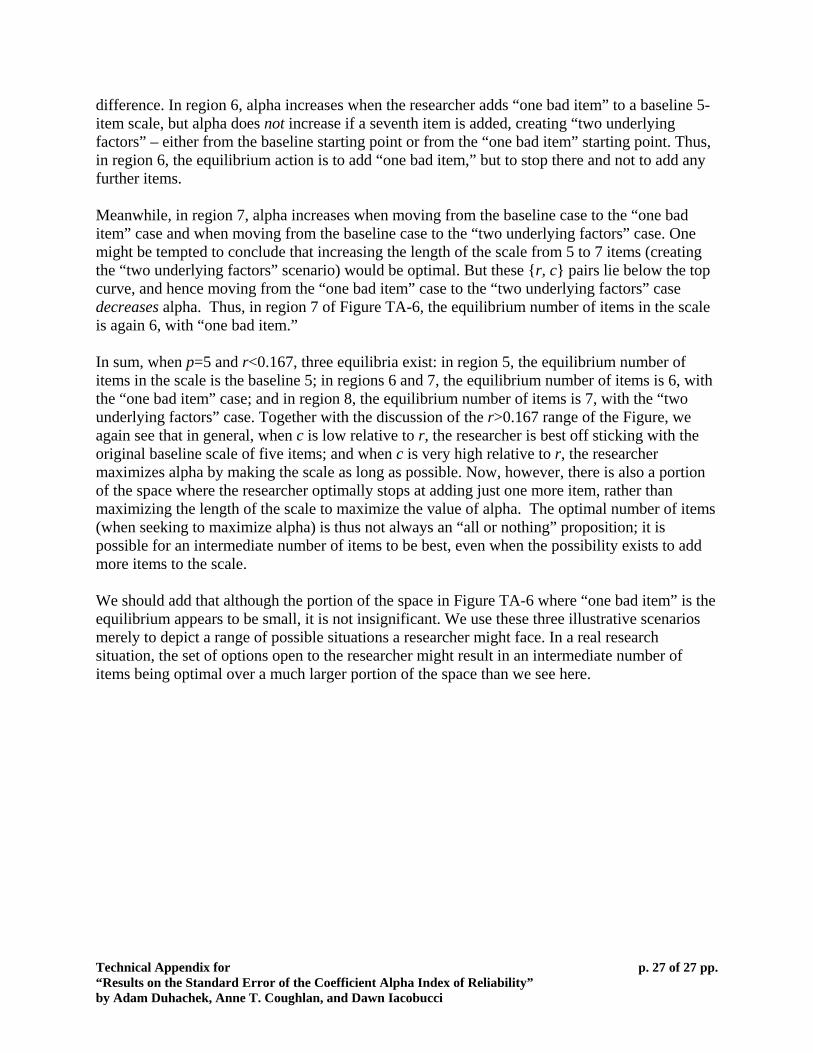
difference. In region 6, alpha increases when the researcher adds “one bad item” to a baseline 5-item scale, but alpha does not increase if a seventh item is added, creating “two underlying factors” – either from the baseline starting point or from the “one bad item” starting point. Thus, in region 6, the equilibrium action is to add “one bad item,” but to stop there and not to add any further items. Meanwhile, in region 7, alpha increases when moving from the baseline case to the “one bad item” case and when moving from the baseline case to the “two underlying factors” case. One might be tempted to conclude that increasing the length of the scale from 5 to 7 items (creating the “two underlying factors” scenario) would be optimal. But these {r, c} pairs lie below the top curve, and hence moving from the “one bad item” case to the “two underlying factors” case decreases alpha. Thus, in region 7 of Figure TA-6, the equilibrium number of items in the scale is again 6, with “one bad item.” In sum, when p=5 and r<0.167, three equilibria exist: in region 5, the equilibrium number of items in the scale is the baseline 5; in regions 6 and 7, the equilibrium number of items is 6, with the “one bad item” case; and in region 8, the equilibrium number of items is 7, with the “two underlying factors” case. Together with the discussion of the r>0.167 range of the Figure, we again see that in general, when c is low relative to r, the researcher is best off sticking with the original baseline scale of five items; and when c is very high relative to r, the researcher maximizes alpha by making the scale as long as possible. Now, however, there is also a portion of the space where the researcher optimally stops at adding just one more item, rather than maximizing the length of the scale to maximize the value of alpha. The optimal number of items (when seeking to maximize alpha) is thus not always an “all or nothing” proposition; it is possible for an intermediate number of items to be best, even when the possibility exists to add more items to the scale. We should add that although the portion of the space in Figure TA-6 where “one bad item” is the equilibrium appears to be small, it is not insignificant. We use these three illustrative scenarios merely to depict a range of possible situations a researcher might face. In a real research situation, the set of options open to the researcher might result in an intermediate number of items being optimal over a much larger portion of the space than we see here.


p. 27 of 27 pp.

Documents

Technical Appendix for - Warringtonbear.warrington.ufl.edu/centers/MKS/appendices/Results on the... · by Adam Duhachek, Anne T. Coughlan, and Dawn Iacobucci p. 4 of 27 pp. substitutes